


1. Introduction
The flow of a composite material consisting of inert non-Brownian solid spheres dispersed in a background viscous fluid clearly differs from both pure fluid flow and the motion of dry grains in a vacuum. When the entrained particles are large enough for thermal fluctuations to be negligible, such composite materials are commonly referred to as suspensions, distinguishing them from colloids. Early theoretical descriptions of the rheology of suspensions treat the material as an effective fluid and aim to describe the influence of the solid spheres on the viscosity. Einstein (Reference Einstein1911) considered a single suspended sphere, derived the energy dissipated by the sphere, and carried out a homogenisation to show that the dependence of the effective viscosity  $\eta$ on the fluid viscosity $\eta _f$ and the solid volume fraction $\phi$ is well approximated by the formula $\eta \approx \eta _f(1+5\phi /2)$, which remains accurate at low solid volume fraction. Subsequent works (Bingham & White Reference Bingham and White1911; Batchelor & Green Reference Batchelor and Green1972) refined this result by using higher-order expansions and by incorporating additional hydrodynamic effects to motivate semi-empirical fits (Krieger & Dougherty Reference Krieger and Dougherty1959). However, whilst it is clear that these theories have the correct limiting behaviour as $\phi \to 0$, they predict unphysical behaviour as $\phi$ is increased because in reality a jamming limit is observed at a critical packing fraction $\phi =\phi _m$, where the effective viscosity apparently tends to infinity (Frankel & Acrivos Reference Frankel and Acrivos1967; Boyer, Guazzelli & Pouliquen Reference Boyer, Guazzelli and Pouliquen2011). Even below this critical value, the interactions between solid particles become increasingly significant and eventually dominant as the jamming limit is approached.
In the past two decades, the understanding and modelling of the solid-phase dynamics in suspensions has been greatly improved, through both experimental and theoretical endeavours. As summarised in the review of Guazzelli & Pouliquen (Reference Guazzelli and Pouliquen2018), there are now a wealth of rheological measurements, in multiple geometries, characterising the dependence of the effective viscosity over the full range of  $\phi$. Amongst these, the experiments of Boyer et al. (Reference Boyer, Guazzelli and Pouliquen2011) stand out as offering an additional level of insight into the role of the particle dynamics. In order to isolate the particle-phase rheology from the mixture response, Boyer et al. (Reference Boyer, Guazzelli and Pouliquen2011) employed a novel shear rheometer in which flow is driven by a top plate that is permeable to liquid but not particles. These experiments allowed for the strain rate $\dot {\gamma }$ and the particle pressure $p$ to be controlled independently while $\phi$ and the bulk friction $\mu$ were measured. The key observation is that at steady state, a dimensionless strain rate, the viscous number
 \begin{equation} J=\frac{\eta_f \dot{\gamma}}{p} , \end{equation}
controls both the effective friction (via a constitutive relation  $\mu =\mu (J)$) and the packing fraction, with a dependence $\phi =\varPhi (J)$. The resulting $\mu (J), \varPhi (J)$ rheology has subsequently been found to be a reliable description of the steady-state particle rheology for suspensions in many geometries (Lecampion & Garagash Reference Lecampion and Garagash2014; Rauter Reference Rauter2021).
The structure of the Boyer et al. (Reference Boyer, Guazzelli and Pouliquen2011)  $\mu (J), \varPhi (J)$ rheology is similar to corresponding models for dry granular materials. For steady granular flow, a different dimensionless strain rate, the inertial number $I$, is observed in experiments to be the controlling variable. The significance of the inertial number inspired the incompressible $\mu (I)$ rheology of Jop, Forterre & Pouliquen (Reference Jop, Forterre and Pouliquen2006), in which $\phi$ is a constant, and the $\mu (I), \varPhi (I)$ rheology of Pouliquen et al. (Reference Pouliquen, Cassar, Jop, Forterre and Nicolas2006), with $\phi =\varPhi (I)$ allowed to vary. The functional forms of the $\mu (J)$ and $\varPhi (J)$ relations proposed by Boyer et al. (Reference Boyer, Guazzelli and Pouliquen2011) share fundamental properties with the $\mu (I),\varPhi (I)$ rheology of dry granular materials. Specifically, $\mu$ is a strictly increasing function in both theories, whereas $\varPhi$ is decreasing, and a static yield stress with $\mu =\mu _1$ and $\phi =\phi _m$ is recovered as $J$ or $I$ tends to zero. These similarities correspond to the property that frictional grain contacts dominate suspension rheology at large solid fractions.
The  $\mu (J),\varPhi (J)$ rheology introduces compressibility of the particle phase by allowing $\phi$ to vary as deformation and motion proceed. However, the relation $\phi =\varPhi (J)$ constrains the evolution and spatial distribution of $\phi$ to depend a priori on the viscous number $J$, independently of other details of the motion. A consequence of this constraint is that, as in the $\mu (I),\varPhi (I)$ rheology for dry granular materials, the resulting equations of motion tend to be dynamically ill-posed (Heyman et al. Reference Heyman, Delannay, Tabuteau and Valance2017; Schaeffer et al. Reference Schaeffer, Barker, Tsuji, Gremaud, Shearer and Gray2019). This unsavoury feature means that high-frequency spatial variations grow exponentially in time, at a rate that depends quadratically on the frequency or wavenumber. Known technically as Hadamard ill-posedness (Hadamard Reference Hadamard1902), this property is investigated by linearising the dynamic equations of motion and characterising the growth rates associated with spatial Fourier modes. As ill-posedness corresponds to unbounded positive growth rates due to the leading-order terms, nonlinear contributions to the stability (see Goddard & Lee Reference Goddard and Lee2017) are insufficient to regularise the behaviour.
These aspects of ill-posedness contrast physically realistic dispersion relations that have pure decay, a finite cut-off or an asymptotic limit. Another significant consequence of dynamic ill-posedness is that although low-resolution numerical simulations are well behaved, grid refinement corresponds to increasing the wavenumber that is accessible by the calculation so that sufficiently high-resolution numerical simulations exhibit large-grid-scale oscillations that are unphysical (see e.g. Barker & Gray Reference Barker and Gray2017; Martin et al. Reference Martin, Ionescu, Mangeney, Bouchut and Farin2017).
Dynamic ill-posedness has long been recognised as a limitation of continuum theories of time-dependent flow of dry granular materials under the assumption that the material is incompressible, so that  $\phi$ is constant (see Pitman & Schaeffer Reference Pitman and Schaeffer1987; Schaeffer Reference Schaeffer1987). Pertinently, Barker et al. (Reference Barker, Schaeffer, Bohorquez and Gray2015) established that the incompressible $\mu (I)$ rheology of Jop et al. (Reference Jop, Forterre and Pouliquen2006) suffers from ill-posedness in specific regimes, notably large or small values of $I$. There was hope that introducing compressibility would stabilise the dynamics, but as demonstrated by Heyman et al. (Reference Heyman, Delannay, Tabuteau and Valance2017), the $\mu (I),\varPhi (I)$ rheology changes the conditions on ill-posedness but does not eliminate it. Similarly, the new analysis in the present paper demonstrates that the $\mu (J), \varPhi (J)$ rheology for suspensions leads to ill-posed equations whenever the viscous number $J$ is below a threshold value $J=J_{crit}$. Since $\phi =\varPhi (J)$ is decreasing, ill-posedness appears for all solid volume fractions above a critical value $\phi _{crit}=\varPhi (J_{crit})$. Because $\phi _{crit}<\phi _m=\varPhi (0)$, the problematic unphysical behaviour of ill-posedness is exhibited by the $\mu (J), \varPhi (J)$ rheology, even before the jamming transition is reached. Crucially, the general aspects of this finding are not limited to the specifics of the $\mu (J),\varPhi (J)$ rheology because, as discussed by Boyer et al. (Reference Boyer, Guazzelli and Pouliquen2011), classical theories in which the effective mixture viscosity is a function of the solid volume fraction only can be reformulated as versions of the $\mu (J),\varPhi (J)$ rheology.
In Barker et al. (Reference Barker, Schaeffer, Shearer and Gray2017) and Schaeffer et al. (Reference Schaeffer, Barker, Tsuji, Gremaud, Shearer and Gray2019), a substantially different approach was introduced by generalising the role of  $\phi$ so that it evolves dynamically in conjunction with invariants of the strain rate and stress tensors. These ideas derive from soil mechanics, in particular the theory of critical-state soil mechanics (Jackson Reference Jackson1983). In Barker et al. (Reference Barker, Schaeffer, Shearer and Gray2017), the Coulomb-type friction law used in the $\mu (I)$ framework was extended to general yield-stress functions, and the strict $\phi =\varPhi (I)$ relation was replaced by a dilatancy rule in which the velocity divergence is specified as a function of the state variables. This new system of equations is called the compressible $I$-dependent rheology (CIDR) and, as shown by Barker et al. (Reference Barker, Schaeffer, Shearer and Gray2017), leads to dynamic equations that are well-posed, in the sense that growth rates of Fourier modes for the linearised equations are bounded above with respect to wavenumber, provided that the constitutive functions are chosen to satisfy specific criteria. In the original formulation, CIDR was intended for dry granular flow beyond the jamming transition $\phi >\phi _m$, in the so-called quasi-static regime. The approach was later successfully reformulated for the inertial regime $\phi <\phi _m$, as iCIDR, in Schaeffer et al. (Reference Schaeffer, Barker, Tsuji, Gremaud, Shearer and Gray2019).
In the present paper, two new versions of CIDR are introduced for the particle-phase rheology in suspensions: vCIDR, which is based around dependence on the viscous number; and viCIDR, which includes both inertial and viscous scalings. In each of these, conditions on the yield condition and dilatancy rule that guarantee well-posedness are formulated that are applicable to all stress states, packing fractions and deformations. Inclusion of the viscous number  $J$ in the CIDR constitutive equations, along with modifying the role of the function $\mu$, changes the analysis significantly, but the resulting conditions guaranteeing well-posedness for vCIDR and viCIDR are each natural generalisations of the results for dry granular materials under CIDR. The dynamic equations with vCIDR are then tested numerically with an initial velocity field that oscillates spatially with large wavenumber. It is shown that calculations using the $\mu (J), \varPhi (J)$ rheology blow up sharply, whereas the vCIDR formulation gives grid-converged results that are independent of the resolution as it is refined. A further test demonstrates that an inhomogeneous initial solid fraction distribution homogenises smoothly over time, even when close to the jamming transition.
In § 2, the tensorial equations of motion of the  $\mu (J),\varPhi (J)$ rheology are introduced as an extension to the dry granular flow equations. These equations are shown to be ill-posed for small values of the viscous number $J$ in § 3. This result is then demonstrated in numerical solutions in § 4. In § 5, ideas from Barker et al. (Reference Barker, Schaeffer, Shearer and Gray2017) are employed to formulate the vCIDR rheology for suspensions, and to show that the equations of motion are well-posed under general conditions on the constitutive functions. This section also includes an illustration of how the yield condition and dilatancy rule can be formulated in order to recover the $\mu (J), \varPhi (J)$ rheology for isochoric deformations, i.e. those for which the flow is steady and the velocity is divergence-free. Numerical simulations in § 6 verify the well-posed behaviour of vCIDR for a shear flow. In § 7, a further generalisation of the theory is made to allow for flows with a wider range of strain rates, including those for which both the viscous number and the inertial number are non-negligible; this theory is named viCIDR.
2. Equations of motion
In this section, the continuum equations for dry granular flow, with  $\mu (I)$ rheology, are summarised alongside the equivalent relations derived from the $\mu (J)$ and $\varPhi (J)$ relations of Boyer et al. (Reference Boyer, Guazzelli and Pouliquen2011) for particles in suspension. The dependent variables in these systems of equations in two space dimensions are the volume fraction of particles $\phi$, the velocity $\boldsymbol {u}=(u_1,u_2)$, and the particle pressure $p$. These functions of spatial variables $(x_1,x_2)$ and time $t$ satisfy the system of partial differential equations (PDEs) representing conservation of mass and momentum, augmented by constitutive laws. From the outset, the partial density of the grains (defined per unit mixture volume) is taken to be $\rho =\rho _*\phi$, where $\rho _*$ is the constant intrinsic density of the solid particles. Allowing for compressibility through $\phi$ variation, conservation of mass is then expressed as
 \begin{equation} \partial _t\phi+\boldsymbol{\nabla} \boldsymbol{\cdot} (\phi\boldsymbol{u})=0, \end{equation}
and conservation of momentum is
 \begin{equation} \rho_*\phi(\partial _t\boldsymbol{u}+(\boldsymbol{u}\boldsymbol{\cdot}\boldsymbol{\nabla} ) \boldsymbol{u})={-}\boldsymbol{\nabla} p + \boldsymbol{\nabla} \boldsymbol{\cdot} \boldsymbol{\tau}+\rho_*\phi \boldsymbol{b} , \end{equation}
where the vector  $\boldsymbol {b}$ represents acceleration due to body forces, such as gravity and drag, and the deviatoric shear-stress tensor $ \boldsymbol{\tau}$ comes from decomposing the two-dimensional Cauchy stress tensor $ \boldsymbol{\sigma}$ as
 \begin{equation} {\sigma}_{ij}={-}p\delta_{ij}+{\tau}_{ij},\quad i,j=1,2. \end{equation}
The equations of motion are supplemented by constitutive equations and assumptions as follows. Alignment of shear stress and strain rate, i.e.
 \begin{equation} \frac{\boldsymbol{\tau}}{\|\boldsymbol{\tau}\|}=\frac{ \boldsymbol{S}}{\| \boldsymbol{S}\|}, \end{equation}
is assumed here, in which  $ \boldsymbol{S}=(S_{ij})$ is the deviatoric part of the strain rate,
 \begin{equation} S_{ij}=\tfrac{1}{2}(\partial _iu_j+\partial _ju_i) - \tfrac{1}{2}(\mathrm{div} \, \boldsymbol{u}) \delta_{ij} , \end{equation}
with second invariant
 \begin{equation} \| \boldsymbol{S}\|=\sqrt{\frac{1}{2} \sum_{i,j=1}^2 S_{ij}^2}, \end{equation}
and the Drucker–Prager type (Lubliner Reference Lubliner1990) yield condition during deformation implies
 \begin{equation} \|\boldsymbol{\tau}\|=\mu p. \end{equation}
If the friction coefficient  $\mu =\mu _s$ is a constant, then this expression is equivalent to the classical Drucker–Prager theory, whereas including dependence on the inertial number
 \begin{equation} I=\frac{2d\,\| \boldsymbol{S}\|}{\sqrt{p/\rho_*}} \end{equation}
leads instead to the  $\mu (I)$ rheology of Jop et al. (Reference Jop, Forterre and Pouliquen2006) for dry granular materials.
2.1. The  $\mu (J), \varPhi (J)$ rheology

To describe the rheology of particles in suspension, Boyer et al. (Reference Boyer, Guazzelli and Pouliquen2011) introduced the viscous number
 \begin{equation} J=\frac{2\eta_f\,\|{\boldsymbol{S}}\|}{p}, \end{equation}
where  $\eta _f$ is the viscosity of the background fluid. Although different from the inertial number $I$,
$I$,  $J$ retains a dependence on the shear rate $\| \boldsymbol{S}\|$ and the particle pressure $p$. It should be noted that both $I$ and $J$ appear to have an extra factor 2 compared to the corresponding definitions in Boyer et al. (Reference Boyer, Guazzelli and Pouliquen2011) due to the connection between $\| {\boldsymbol{S}}\|$ and the classical scalar shear rate: $\dot {\gamma }=2\| \boldsymbol{S}\|$.
As demonstrated by Boyer et al. (Reference Boyer, Guazzelli and Pouliquen2011), steady isochoric shear flows have  $\mu =\mu (J)$, with an increasing and unbounded function, with a proposed form
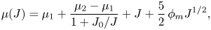 \begin{equation} \mu(J)=\mu_1+\frac{\mu_2-\mu_1}{1+J_0/J}+J+\frac52\,\phi_mJ^{1/2}, \end{equation}
which involves a contact contribution (the first two terms) and a hydrodynamic part (the last two terms). Combining the  $\mu (J)$ relation with the yield condition (2.7) and alignment (2.4) specifies the shear-stress tensor
 \begin{equation} \boldsymbol{\tau} = \frac{\mu(J)\,p}{\|\boldsymbol{S}\|}\boldsymbol{S}, \end{equation}
which defines an effective non-Newtonian viscosity for the suspension
 \begin{equation} \eta_s = \frac{\mu(J) p}{2\|{\boldsymbol{S}}\|}. \end{equation}
In component form, conservation of momentum becomes
 \begin{equation} \rho_*\phi(\partial _t u_i+u_j\partial _j u_i)=\partial _j\left[\frac{\mu(J)\,p}{\| \boldsymbol{S}\|}\,S_{ij}\right]-\partial _ip+\rho_*\phi b_i, \quad i=1,2 . \end{equation}
Compressibility in Boyer et al. (Reference Boyer, Guazzelli and Pouliquen2011) is included as a constitutive equation by tying  $\phi$ to the viscous number:
 \begin{equation} \phi=\varPhi(J), \end{equation}
with  $\varPhi$ being a strictly decreasing function of $J$. A well-established form for $\varPhi$ is
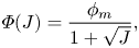 \begin{equation} \varPhi(J) = \frac{\phi_m}{1+\sqrt{J}} , \end{equation}
with inverse function  $\mathcal {J}:$
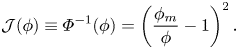 \begin{equation} \mathcal{J}(\phi) \equiv \varPhi^{{-}1}(\phi) = \left(\frac{\phi_m}{\phi}-1 \right)^2. \end{equation}
Typical parameters for these constitutive relations are given in table 1. Solving (2.9) for  $p$ and using $J=\mathcal {J}(\phi )$ gives
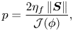 \begin{equation} p = \frac{2\eta_f\,\|{\boldsymbol{S}}\|}{\mathcal{J}(\phi)} , \end{equation}
i.e. an equation of state in which stresses depend on the second invariant of the strain rate tensor and the solid volume fraction.
Table 1. Model parameters from Boyer et al. (Reference Boyer, Guazzelli and Pouliquen2011) that characterise steady uniform flow in their three-dimensional experiments.
3. Analysis of well-posedness for the Boyer et al. (Reference Boyer, Guazzelli and Pouliquen2011) model
Here, it is shown that the  $\mu (J), \varPhi (J)$ equations are well-posed only when $\mu (J)>1$. As demonstrated in § 4, the loss of well-posedness at low viscous number (i.e. high confining pressure or small strain rate) has catastrophic implications for high-resolution numerical simulations of time-dependent flow, even though low-resolution simulations may appear to be well-behaved. Given (2.10), the constraint for well-posedness is equivalent to requiring $J>J_{crit}$, where for the parameters given in table 1, the critical value is $J_{crit}\approx 0.0417$. Similarly, (2.15) implies a corresponding maximal volume fraction
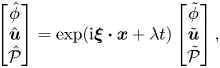
  $\phi =\phi _{crit}=\varPhi (J_{crit})\approx 0.486$, above which the equations are predicted to be ill-posed. This partitioning of the parameter space is shown graphically in figure 1.
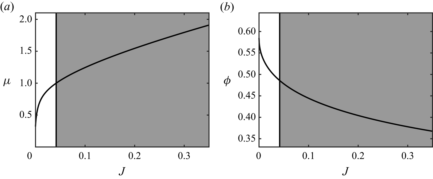
Figure 1. The ill-posed white region and well-posed grey region for the  $\mu (J), \varPhi (J)$ rheology of Boyer et al. (Reference Boyer, Guazzelli and Pouliquen2011). Vertical black lines are the neutral stability point at $J=J_{crit}\approx 0.0417$, and the curves are the relations (2.10) and (2.15) with parameters given in table 1.
3.1. Linearisation of the equations
Equations (2.1) and (2.13) are linearised by appealing to Barker et al. (Reference Barker, Schaeffer, Bohorquez and Gray2015) for some of the manipulations that simplify the calculation. Note that  $\phi$ is retained as an evolving variable, whereas in (2.13), $\mu =\mu (J)$. Retaining this point of view, the constitutive law
 \begin{equation} \phi=\varPhi(J) \end{equation}
is linearised rather than substituting (3.1) into the PDE system. Consequently, the variables are  $\phi, \boldsymbol {u}, p$. As the intrinsic density $\rho _*$ is constant, it is actually more compact in the following to work instead with the scaled pressure
 \begin{equation} \mathcal{P}=\frac{p}{\rho_*}, \end{equation}
in effect dividing both sides of the momentum balance (2.13) by  $\rho _*$. The new variables are perturbed about a base state $\phi ^0=\varPhi (J^0)$, $\boldsymbol {u}^0$, $\mathcal {P}^0$, in which $J=J^0$ is given by (2.9) with $p=\rho _*\mathcal {P}$, so that
 \begin{equation} \phi=\phi^0+\hat{\phi},\quad \boldsymbol{u}=\boldsymbol{u}^0+\hat{\boldsymbol{u}}, \quad \mathcal{P}=\mathcal{P}^0+\hat{\mathcal{P}}. \end{equation}
The base state can vary in space, but coefficients involving the base state will be treated as constant, which is consistent with high wavenumber behaviour. Substituting into the equations and retaining terms linear in the perturbed fields means that, for instance, mass balance (2.1) reduces to
 \begin{equation} \partial _t \hat{\phi}+\phi^0\,\boldsymbol{\nabla} \boldsymbol{\cdot}\hat{\boldsymbol{u}}+\boldsymbol{u}^0\boldsymbol{\cdot}\boldsymbol{\nabla} \hat{\phi}=0. \end{equation}
Note that some terms, such as  $\hat {\phi }\,\boldsymbol {\nabla } \boldsymbol {\cdot }\boldsymbol {u}^0$, have been dropped since this term will be dominated at high wavenumber by the term $\boldsymbol {u}^0\boldsymbol {\cdot }\boldsymbol {\nabla } \hat {\phi }$, which has derivative $\hat {\phi }$. This elimination has been carried out with other terms in this equation, and will also be made in what follows to avoid cluttering the calculation with unnecessary terms. In fact, through this process, only the terms that contribute to the principal part of the linearised equations are retained. It is also convenient to write (3.4) in component form:
 \begin{equation} \partial _t \hat{\phi}+\phi^0\,\partial _j\hat{u}_j+{u}^0_j\,\partial _j\hat{\phi}=0. \end{equation}
 To linearise the momentum equation (2.13), there is a complicated collection of the linearisations of nonlinear terms. These are essentially executed in Barker et al. (Reference Barker, Schaeffer, Bohorquez and Gray2015), except that in that paper, use is made of the assumption of incompressibility,  $\boldsymbol {\nabla } \boldsymbol {\cdot } \boldsymbol {u}=0$, and the non-dimensional strain rate is different, resulting in slightly different formulas. In the case of the $\mu (J), \varPhi (J)$ rheology, some useful derivations (summing repeated indices here and elsewhere) are
 \begin{equation} \partial _j S_{ij}=\frac{1}{2}\,\partial _{jj} u_i \ (i=1,2), \quad \partial _{\mathcal{P}} J={-}\frac{J}{\mathcal{P}}, \quad \partial _{\| \boldsymbol{S}\|}J=\frac{J}{\| \boldsymbol{S}\|}. \end{equation}
As in Barker et al. (Reference Barker, Schaeffer, Bohorquez and Gray2015), quantities determined from the base state are introduced, including the normalized strain rate tensor  $ \boldsymbol{A}=(A_{ij})$:
 \begin{equation} \boldsymbol{A}=\frac{ \boldsymbol{S}}{\| \boldsymbol{S}\|}, \quad \eta^0=\frac{\mu \mathcal{P}^0}{2\| \boldsymbol{S}\|},\quad \nu=\frac{J^0\,\mu'(J^0)}{\mu(J^0)}, \quad q=\mu(1-\nu),\quad r=1-\nu. \end{equation}
Given these, the principal part of the linearisation of the momentum equations can be written as
 \begin{equation} \phi^0\,\partial _t \hat{u}_i=\eta^0[\partial _{jj} \hat{u}_i-rA_{ij}A_{kl}\,\partial _j\partial _l\hat{u}_k]+ [qA_{ij}\,\partial _j-\partial _i ]\hat{\mathcal{P}} +\hat{\phi} b_i. \end{equation}
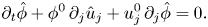
Finally, to complete the leading-order system, (3.1) is linearised, bearing in mind that  $J$ depends on the dependent variables. Thus
 \begin{equation} \hat{\phi}=\varPhi'(J^0)\left[ \frac{J^0}{4\| \boldsymbol{S}\|}\,A_{jk}(\partial _j \hat{u}_k+\partial _k\hat{u}_j)-\frac{J^0}{\mathcal{P}^0}\,\hat{\mathcal{P}}\right]. \end{equation}
3.2. Eigenvalue problem
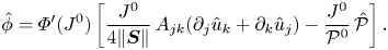
In the next step, the coefficients in the linear system (3.5), (3.8) and (3.9) are frozen and solutions of the normal mode form
 \begin{equation} \left[\begin{array}{@{}c@{}} \hat{\phi}\\ \hat{\boldsymbol{u}}\\ \hat{\mathcal{P}} \end{array} \right] =\exp({\rm i}\boldsymbol{\xi}\boldsymbol{\cdot}\boldsymbol{x}+\lambda t)\left[\begin{array}{@{}c@{}} \tilde{\phi}\\ \tilde{\boldsymbol{u}}\\ \tilde{\mathcal{P}} \end{array} \right], \end{equation}
with constants  $\tilde {\phi }$, $\tilde {\boldsymbol {u}}$ and $\tilde {\mathcal {P}}$, are sought. Here, $\boldsymbol {\xi }$ is the spatial wavenumber, and $\lambda$ is the temporal growth or decay rate. Substituting into (3.5), (3.8) and (3.9), a generalised eigenvalue problem is recovered (dropping the superscript $0$ from the base state as in Barker et al. (Reference Barker, Schaeffer, Bohorquez and Gray2015) for brevity):
 $$\begin{gather} \lambda\tilde{\phi}+{\rm i}\phi\xi_j\tilde{u}_j+{\rm i}{u}_j\xi_j\tilde{\phi}=0, \end{gather}$$
 $$\begin{gather}\phi\lambda\tilde{u}_i=\eta[-|\xi|^2\tilde{u}_i +rA_{ij}A_{kl}\xi_j\xi_l\tilde{u}_k]+{\rm i}[qA_{ij}\xi_j-\xi_i ]\tilde{\mathcal{P}}+\tilde{\phi}b_i, \end{gather}$$
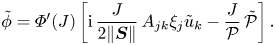 $$\begin{gather}\tilde{\phi}=\varPhi'(J)\left[{\rm i}\,\frac{J}{2\| \boldsymbol{S}\|}\,A_{jk}\xi_j\tilde{u}_k-\frac{J}{\mathcal{P}}\,\tilde{\mathcal{P}}\right]. \end{gather}$$
These equations form a  $4\times 4$ generalised eigenvalue problem for $\lambda =\lambda (\boldsymbol {\xi })$. It is convenient to rotate the coordinates $\boldsymbol {\xi }$ to diagonalise the trace-free symmetric matrix $\boldsymbol{A}$, so that one may take (since $\| \boldsymbol{A}\|=1$)
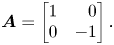 \begin{equation} \boldsymbol{A}=\left[ \begin{array}{@{}rr@{}} 1 & 0\\ 0 & -1 \end{array} \right]. \end{equation}
Naturally, this greatly simplifies the equations:
 $$\begin{gather} \lambda\tilde{\phi}+{\rm i}\phi\xi_j\tilde{u}_j+{\rm i}{u}_j\xi_j\tilde{\phi}=0, \end{gather}$$
 $$\begin{gather}\phi\lambda\tilde{u}_1=\eta[ -|\xi|^2\tilde{u}_1+r \xi_1(\xi_1\tilde{u}_1-\xi_2\tilde{u}_2)] +{\rm i}(q-1)\xi_1\tilde{\mathcal{P}}+\tilde{\phi}b_1, \end{gather}$$
 $$\begin{gather}\phi\lambda\tilde{u}_2=\eta[ -|\xi|^2\tilde{u}_2-r\xi_2(\xi_1\tilde{u}_1-\xi_2\tilde{u}_2)] -{\rm i}(q+1)\xi_2 \tilde{\mathcal{P}}+\tilde{\phi}b_2, \end{gather}$$
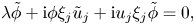
 $$\begin{gather}\tilde{\phi}=\varPhi'(J)\left[{\rm i}\,\frac{J}{2\| \boldsymbol{S}\|}\,(\xi_1 \tilde{u}_1-\xi_2\tilde{u}_2)-\frac{J}{\mathcal{P}}\,\tilde{\mathcal{P}}\right]. \end{gather}$$
To find the values of  $\lambda$ for which the system has non-trivial solutions, characteristic equation $\det B(\lambda,\xi )=0$ is solved, where $B(\lambda,\xi )$ is the coefficient matrix for the system:
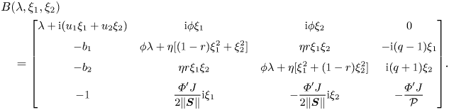 \begin{align} &
B(\lambda,\xi_1,\xi_2) \nonumber\\
&\quad = \small{\left[\begin{array}{@{}cccc@{}} \lambda + {\rm i}(u_1\xi_1+u_2\xi_2) &
{\rm i}\phi\xi_1 & {\rm i}\phi\xi_2 & 0\\
-b_1 & \phi\lambda+ \eta[(1-r)\xi_1^2 +\xi_2^2] & \eta r\xi_1\xi_2 & -{\rm i}(q-1)\xi_1\\
-b_2 & \eta r\xi_1\xi_2 & \phi\lambda+ \eta [\xi_1^2+(1-r)\xi_2^2] & {\rm i}(q+1)\xi_2\\
-1 & \dfrac{\varPhi'J}{2\| \boldsymbol{S}\|}{\rm i}\xi_1 & - \dfrac{\varPhi'J}{2\| \boldsymbol{S}\|}{\rm i}\xi_2 &
-\dfrac{\varPhi'J}{\mathcal{P}} \end{array} \right]}.
\end{align}
\begin{align} &
B(\lambda,\xi_1,\xi_2) \nonumber\\
&\quad = \small{\left[\begin{array}{@{}cccc@{}} \lambda + {\rm i}(u_1\xi_1+u_2\xi_2) &
{\rm i}\phi\xi_1 & {\rm i}\phi\xi_2 & 0\\
-b_1 & \phi\lambda+ \eta[(1-r)\xi_1^2 +\xi_2^2] & \eta r\xi_1\xi_2 & -{\rm i}(q-1)\xi_1\\
-b_2 & \eta r\xi_1\xi_2 & \phi\lambda+ \eta [\xi_1^2+(1-r)\xi_2^2] & {\rm i}(q+1)\xi_2\\
-1 & \dfrac{\varPhi'J}{2\| \boldsymbol{S}\|}{\rm i}\xi_1 & - \dfrac{\varPhi'J}{2\| \boldsymbol{S}\|}{\rm i}\xi_2 &
-\dfrac{\varPhi'J}{\mathcal{P}} \end{array} \right]}.
\end{align}
The terms with  $u_j, b_j$, $j=1,2$, do not contribute to the high-frequency regime, so these constants are set to zero. In particular, inclusion of body forces with arbitrary dependence on the flow variables, but not their gradients, does not affect this derivation. This may be important when modelling, for example, drag forces between fluid and particles.
After some simplification, this leads to a cubic equation for  $\lambda$:
 \begin{align} \det(B)&= {2\,\frac{a{\phi}^{2}}{\mathcal{P}}\,{\lambda}^{3}} -{\frac{a \phi}{{\| \boldsymbol{S}\|} \mathcal{P}}}\,{k}^{2} [ 2{\| \boldsymbol{S}\|}\eta (r-2)+\mathcal{P}(\cos (2\theta) -q) ] {\lambda}^{2}\nonumber\\ &\quad + \left(\frac {a\eta}{{\| \boldsymbol{S}\|}\mathcal{P}}\,{k}^{4} [ 2{\| \boldsymbol{S}\|} \eta(1-r)+\mathcal{P}(q-\cos (2\theta))] - {\phi}^{2}{k}^{2} [ 1- q \cos(2\theta) ]\right) \lambda \nonumber\\ &\quad + \phi \eta {k}^{4}[1-r\sin^2(2\theta)-q \cos(2\theta)]=0, \end{align}
where  $a=-{\varPhi 'J}/{2}> 0$ for $J>0$, $\xi _1=k\cos \theta$, $\xi _2=k\sin \theta$.
Equation (3.20) is conveniently written as a polynomial in  $\lambda$:
 \begin{equation} a c_1\lambda^3 + a c_2 k^2 \lambda^2 + a c_3 k^4 \lambda + c_4 k^2 \lambda + c_5 k^4 =0, \end{equation}
in which the coefficients  $c_j$, $j=1,\ldots, 5$, depend on the parameters $\eta,q,r$ given by (3.7):
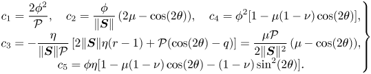 \begin{align}
\left.\begin{array}{@{}c@{}} \displaystyle c_1= \dfrac
{2{\phi}^{2}}{\mathcal{P}}, \quad c_2 ={\dfrac {
\phi}{{\| \boldsymbol{S}\|}}}\,(2\mu - \cos(2\theta)), \quad c_4 =
\phi^2 [ 1- \mu(1-\nu) \cos(2\theta) ], \\
\displaystyle c_3={-}\dfrac {\eta}{{\| \boldsymbol{S}\|}
\mathcal{P}}\,[ 2{\| \boldsymbol{S}\|} \eta
(r-1)+\mathcal{P}(\cos (2\theta) -q)]= \dfrac {\mu
\mathcal{P}}{{ 2\| \boldsymbol{S}\|^2}}\,(\mu-\cos(2\theta)),\\ c_5=
\phi \eta[1- \mu(1-\nu) \cos(2\theta)
-(1-\nu)\sin^2(2\theta) ].
\end{array}\right\}
\end{align}
\begin{align}
\left.\begin{array}{@{}c@{}} \displaystyle c_1= \dfrac
{2{\phi}^{2}}{\mathcal{P}}, \quad c_2 ={\dfrac {
\phi}{{\| \boldsymbol{S}\|}}}\,(2\mu - \cos(2\theta)), \quad c_4 =
\phi^2 [ 1- \mu(1-\nu) \cos(2\theta) ], \\
\displaystyle c_3={-}\dfrac {\eta}{{\| \boldsymbol{S}\|}
\mathcal{P}}\,[ 2{\| \boldsymbol{S}\|} \eta
(r-1)+\mathcal{P}(\cos (2\theta) -q)]= \dfrac {\mu
\mathcal{P}}{{ 2\| \boldsymbol{S}\|^2}}\,(\mu-\cos(2\theta)),\\ c_5=
\phi \eta[1- \mu(1-\nu) \cos(2\theta)
-(1-\nu)\sin^2(2\theta) ].
\end{array}\right\}
\end{align} The signs of the coefficients are now apparent:  $c_1>0$, and $c_2$ changes sign as a function of $\theta$ if and only if $\mu <\frac 12$, otherwise $c_2\geq 0$. Coefficient $c_3$ changes sign in intervals around $\theta =0$ and $\theta ={\rm \pi}$ if $\mu <1$, and otherwise (for $\mu >1$) remains positive. The coefficient $c_5$ is significant in the incompressible limit $a\to 0$, and may change sign in a narrow interval of $\theta$. This occurs because $\nu >0$ approaches zero as $J\to 0$, and tends to unity as $J\to \infty$. Close to these limits, $c_5$ changes sign for $\theta$ in an interval around $\theta ={\rm \pi} /4$. This behaviour corresponds to the analysis of the incompressible granular equations in Barker et al. (Reference Barker, Schaeffer, Bohorquez and Gray2015).
Of the three eigenvalues  $\lambda$ when $a>0$, one is $O(1)$ to leading order (and hence bounded), and two are $O(k^2)$. To see this, consider the asymptotic expansion of $\lambda$ as a function of $k$ as $k\to \infty$, bearing in mind that all the coefficients in (3.21) are powers of $k^2$:
 \begin{equation} \lambda=b_2 k^2+b_0+b_{{-}2} k^{{-}2} + \cdots, \quad k\to \infty . \end{equation}
Substituting into (3.21), we see that (with  $a>0$) the leading-order terms are either $O(k^4)$, when $b_2= 0$, or $O(k^6)$, when $b_2\neq 0$. In the first case, $\lambda =-c_5/(ac_3)+O(k^{-2})$ is a constant to leading order. In the second case, the dominant terms are the first three in the equation, thus $b_2\neq 0$ satisfies the quadratic equation $c_1b_2^2 + c_2b_2 + c_3 =0$, for which the two solutions are real and explicit, leading to the two values of $\lambda$ to $O(k^2)$:
 \begin{equation} \lambda_1(\boldsymbol{\xi})={-}\frac{\mathcal{P}\mu}{2\phi\| \boldsymbol{S}\|}\,k^2<0 \quad \mbox{and} \quad \lambda_2(\boldsymbol{\xi})= \frac{\mathcal{P}}{\phi\| \boldsymbol{S}\|}\,(\cos(2\theta)-\mu)k^2. \end{equation}
Incidentally, in this asymptotic analysis of (3.21), we observe that the fourth term is lower order in both cases  $\lambda \sim b_0$ and $\lambda \sim b_2 k^2$. For the incompressible granular flow mentioned earlier, $a\to 0$, and there is a single eigenvalue, which to leading order is $\lambda =-(c_5/c_4)k^2$. Here, the signs of $c_4$ and $c_5$ are significant and are analysed in Barker et al. (Reference Barker, Schaeffer, Bohorquez and Gray2015).
From (3.24b), we observe that the system is linearly ill-posed if and only if there are wavenumber angles  $\theta$ satisfying $\cos (2\theta )-\mu >0$, which is equivalent to requiring $\mu (J)\geq 1$ for well-posedness. The range of ill-posed directions, when $\mu < 1$, is represented graphically in figure 2. Summarising the result for the $\mu (J), \varPhi (J)$ rheology: assuming $\varPhi '(J)<0$, the system of (2.1) and (2.13) is ill-posed in the regime where $\mu (J)<1$. Conversely, for $\mu (J)>1$, all eigenvalues are real and bounded for all sufficiently large wavenumbers, and are therefore globally bounded as functions of wavenumber. Consequently, the equations are well-posed for viscous numbers $J$ in this regime. Taking typical parameters given in table 1, the implications of this condition are now elaborated. Given (2.10), the ill-posedness condition $\mu (J)<1$ is equivalent to $J< J_{crit}$, where for the parameters given in table 1, $J_{crit}\approx 0.0417$. Similarly, (2.15) gives a corresponding maximal volume fraction $\phi =\phi _{crit}=\varPhi (J_{crit})\approx 0.486$ above which the equations are ill-posed. These conditions, and the related ranges of ill-posedness and well-posedness, are shown in figure 1.
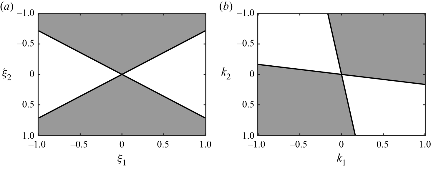
Figure 2. White regions containing ill-posed perturbation directions, and grey regions with decaying modes for the  $\mu (J), \varPhi (J)$ rheology, separated by black neutral curves. (a) System (3.14), chosen for algebraic ease. (b) Here, $ {\boldsymbol{A}}=[0,1;1,0]$, which describes planar shearing. We choose $\mu =\mu _1$ for illustrative purposes.
4. Numerical solutions in a volume-controlled shear cell
Similarly to the experiments of Boyer et al. (Reference Boyer, Guazzelli and Pouliquen2011), flow in a parallel-plate shear cell is considered here. The assumption is that the fields are invariant of the driving direction  $x$ and depend only on the perpendicular coordinate $z$. The flow is driven by a top plate moving at speed $V$ at $z=h$, and the bottom at $z=0$ is held static. Here, the cell height $h$ is fixed, so that the volume of material is a constant in this semi-infinite domain. Introducing the scalings
 \begin{equation} \left.\begin{array}{@{}c@{}} (x,z)=h(\tilde x,\tilde z),\quad (u,w)=V(\tilde u,\tilde w),\quad \boldsymbol{S}=(V/h)\tilde{\boldsymbol{S}},\\ t=(h/V)\tilde t,\quad (p,\boldsymbol{\tau})=\rho_*V^2(\tilde p, \tilde{\boldsymbol{\tau}}), \end{array}\right\} \end{equation}
the resultant one-dimensional solutions for  $\phi (z,t)$ and the non-dimensional velocities $\tilde u(z,t)$ and $\tilde w(z,t)$ (in the $\tilde x$ and $\tilde z$ directions, respectively) satisfy mass conservation
 \begin{equation} \frac{\partial \phi}{\partial \tilde t} ={-}\tilde w\,\frac{\partial \phi}{\partial \tilde z} - \phi\,\frac{\partial \tilde w}{\partial \tilde z}, \end{equation}
and momentum balances in  $\tilde x$,
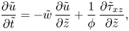 \begin{equation} \frac{\partial \tilde u}{\partial \tilde t} ={-}\tilde w\,\frac{\partial \tilde u}{\partial \tilde z} + \frac{1}{\phi}\,\frac{\partial \tilde{\tau}_{xz}}{\partial \tilde z}, \end{equation}
and in  $\tilde z$,
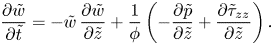 \begin{equation} \frac{\partial \tilde w}{\partial \tilde t} ={-}\tilde w\,\frac{\partial \tilde w}{\partial \tilde z} + \frac{1}{\phi}\left(-\frac{\partial \tilde p}{\partial \tilde z}+\frac{\partial \tilde{\tau}_{zz}}{\partial \tilde z}\right). \end{equation}
These equations are then closed using the constitutive laws (2.7) and (2.17), which specify the shear-stress components and the pressure in terms of  $\phi$ and gradients of the velocities. In non-dimensional variables, these become
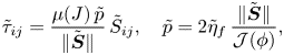 \begin{equation} \tilde{\tau}_{ij} = \frac{\mu(J)\,\tilde p}{\|\tilde{{\boldsymbol{S}}}\|}\,\tilde{S}_{ij}, \quad \tilde p = 2 \tilde{\eta}_f\,\frac{\|\tilde{\boldsymbol{S}}\|}{\mathcal{J}(\phi)}, \end{equation}
where the non-dimensional viscosity is
 \begin{equation} \tilde{\eta}_f =\frac{\eta_f}{\rho_* Vh}. \end{equation}
To drive the flow and conserve mass, the no-slip and no-penetration conditions in non-dimensional variables become
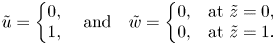 \begin{equation} \tilde u=\left\{\begin{array}{@{}l@{}} 0, \\ 1, \end{array}\right. \quad \mbox{and} \quad \tilde w=\left\{\begin{array}{@{}ll@{}} 0, & \text{at } \tilde z=0,\\ 0, & \text{at } \tilde z=1. \end{array}\right. \end{equation}
It should be noted that the full solid pressure  $p$ is employed here, and in everything that follows, rather than the scaled pressure $\mathcal {P}$ defined in (3.2).
A trivial steady solution exists that has uniform volume fraction  $\phi =\phi _0$, linear shearing $\tilde u=\tilde z$, and no vertical motion $\tilde w=0$. This solution is expected to be stable, representing the long-time behaviour of solutions with appropriate boundary conditions and for arbitrary perturbations of the steady solution as initial data. The transient behaviour away from this case is explored here numerically using the method of lines (MOL) algorithm (Schiesser Reference Schiesser2012) as developed and employed in Schaeffer et al. (Reference Schaeffer, Barker, Tsuji, Gremaud, Shearer and Gray2019). This code takes first-order finite differences for the spatial gradients in the PDEs, generating a system of coupled ordinary differential equations. These are then solved in time using MATLAB's ODE15s routine, which enables fast convergence (typically in seconds) due to the variable-step, variable-order aspects of the algorithm.
The initial conditions for all of the cases considered in this section consist of a small perturbation in  $w$ away from the steady linear shearing solution
 \begin{equation} \tilde u(\tilde z,\tilde t=0) = \tilde z, \quad \tilde w(\tilde z,\tilde t=0) = \epsilon \sin(k\tilde z), \quad \phi(\tilde z,\tilde t=0) = \phi_0, \end{equation}
where  $\epsilon$ is a small parameter and $k$ is a chosen wavenumber. As shown in figures 3 and 4, these initial data can lead to different temporal behaviour, depending on the mean solid volume fraction $\phi _0$ and the grid resolution, quantified here by the number of nodes per wavelength
 \begin{equation} N_\lambda = \frac{N_z}{k} , \end{equation}
where  $N_z$ is the total number of grid points in $0\leq \tilde z \leq 1$.
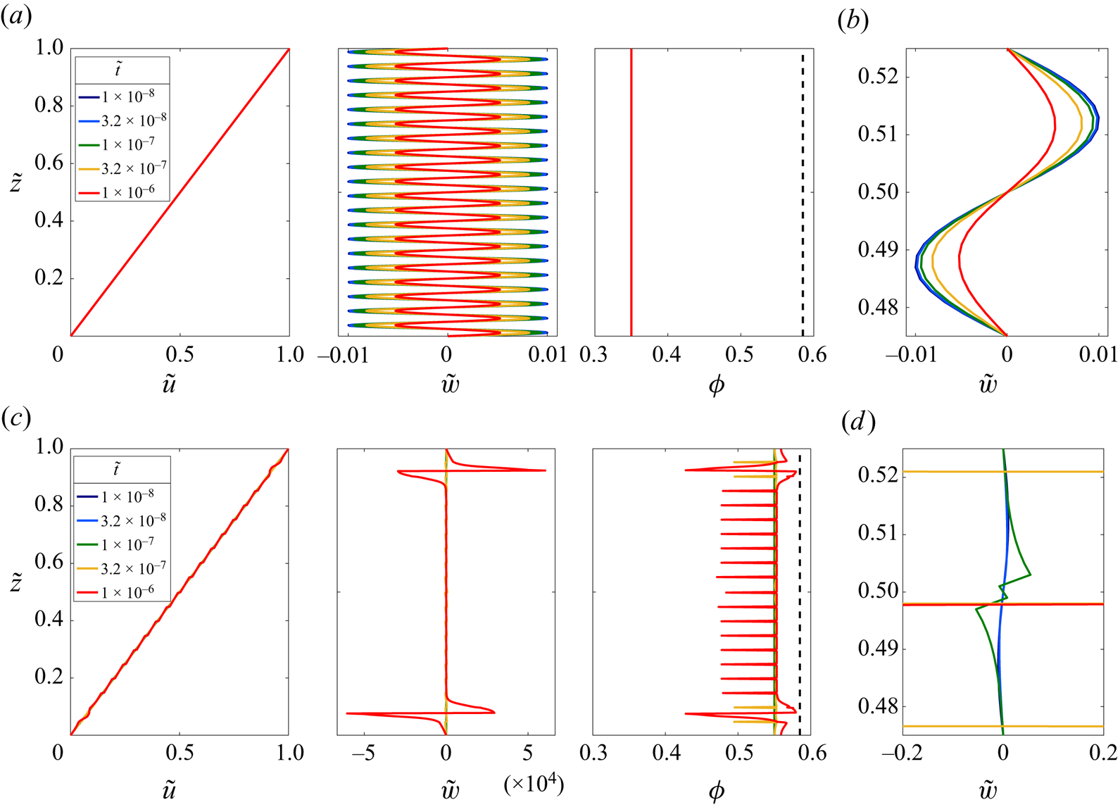
Figure 3. Snapshots of the flow fields as functions of the vertical coordinate  $\tilde {z}$ at progressive times in simulations with the same initial perturbation (4.8) ( $\epsilon =0.01$, $k=40{\rm \pi}$), grid resolution $N_\lambda =25$, and non-dimensional fluid viscosity $\tilde {\eta }_f =3.1$. Panels (a,b) are for the well-posed case $\phi _0=0.35$, and (c,d) are for an ill-posed initial packing fraction $\phi _0=0.55$. Note that the output times are different for each case as the ill-posed simulation fails at $\tilde t\approx 1.08\times 10^{-6}$. Panels (b) and (d) are of the same vertical velocity fields as in (a) and (c), respectively, but zoomed into the centre of the domain in a range spanning one wavelength of the initial perturbation. Animations of these computations can be found in supplementary movies 1 and 2, available at https://doi.org/10.1017/jfm.2022.1004, and plots of the full transient evolution are given in figure 4.
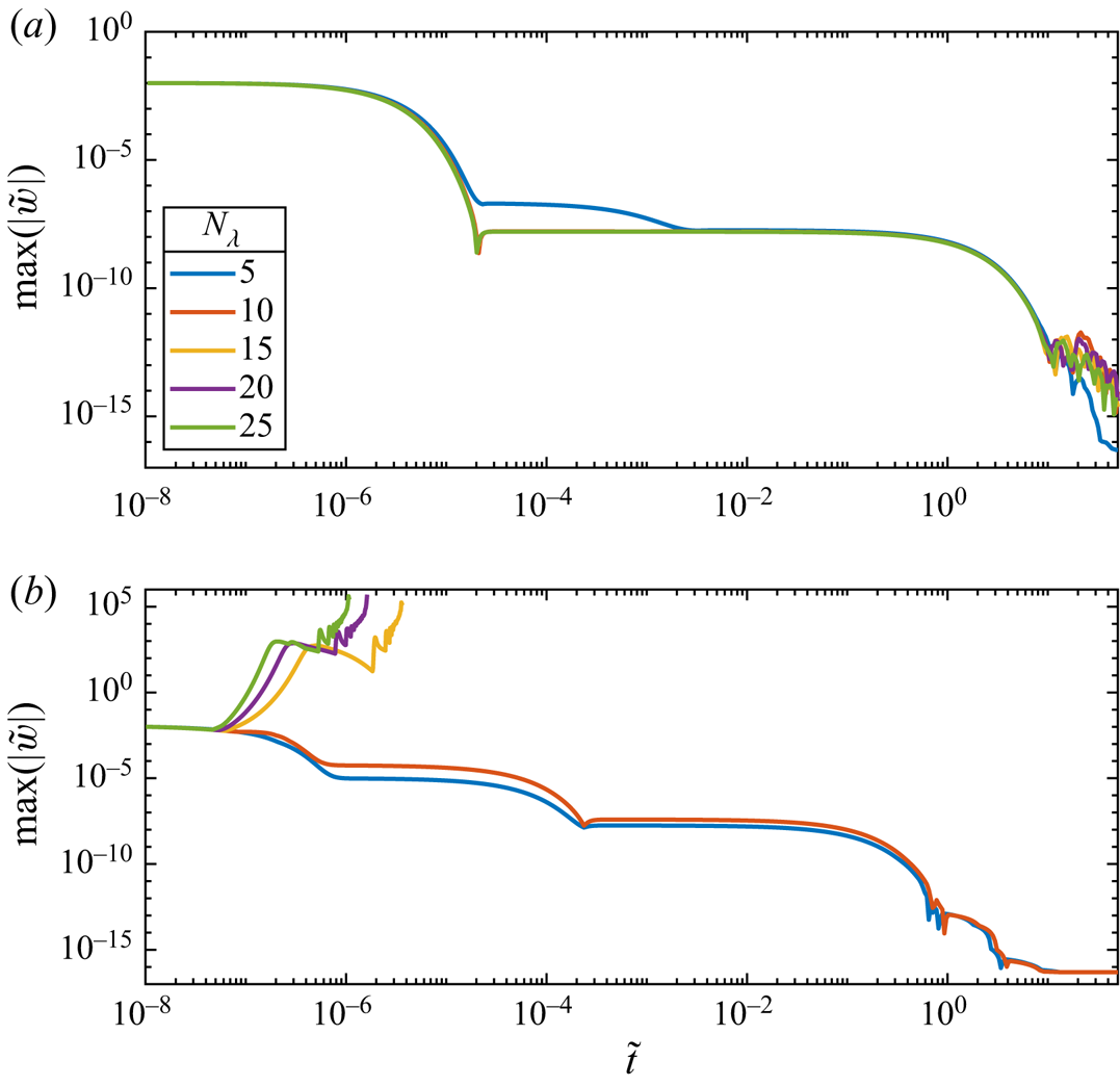
Figure 4. Comparison of the temporal behaviour of the maximum amplitude of  $\tilde w$ at different spatial resolutions with the $\mu (J),\varPhi (J)$ rheology. The cases with $N_\lambda =25$ are those from figure 3. All cases have the same initial perturbation (4.8) with $\epsilon =0.01$ and $k=40{\rm \pi}$. Panel (a) is for $\phi _0=0.35$, which lies in the well-posed range, whereas (b) has $\phi _0=0.55$, which gives ill-posed equations.
As detailed in figures 3(a,b) and 4(a), the solutions exhibit convergence towards the steady solution for the well-posed case  $\phi _0<\phi _{crit}$. Conversely, when $\phi _0>\phi _{crit}$, there is extreme grid dependence, with higher resolutions showing a fast divergence, as plotted in figures 3(c,d) and 4(b), which is a clear indication that the equations being solved are ill-posed.
5. CIDR for viscous flow: vCIDR
In the context of dry granular flow, a similar argument to that of § 3 shows that the  $\mu (I),\varPhi (I)$ rheology proposed in Pouliquen et al. (Reference Pouliquen, Cassar, Jop, Forterre and Nicolas2006) also leads to ill-posed dynamic equations whenever the flow fields satisfy a certain condition, one that cannot be avoided in general flow conditions. Indeed, the result is published in the papers of Heyman et al. (Reference Heyman, Delannay, Tabuteau and Valance2017) and Schaeffer et al. (Reference Schaeffer, Barker, Tsuji, Gremaud, Shearer and Gray2019). However, in Barker et al. (Reference Barker, Schaeffer, Shearer and Gray2017), it was shown how to formulate compressible granular flow equations that are well-posed for all flows, by replacing the $\phi =\varPhi (I)$ constraint by a suitably chosen dilatancy rule. The resulting general theory, called compressible $I$-dependent rheology (CIDR), allows for many different specific choices for the yield-stress and dilatancy functions. In this section, well-posed equations for suspensions are derived using the approach of CIDR. The new yield condition and dilatancy rule, which are defined by this procedure, are given alongside prototype choices for their functional forms. The new theory, for suspensions, is denoted as vCIDR (‘viscous CIDR’).
For vCIDR, the yield condition (2.7) is replaced by a more general form,
 \begin{equation} \|\boldsymbol{\tau}\|=Y(p,\phi,J), \end{equation}
and compressibility is governed by a dilatancy rule (cf. Pailha & Pouliquen Reference Pailha and Pouliquen2009)
 \begin{equation} \mbox{div} \,\boldsymbol{u}=2\,f(p,\phi,J)\,\| \boldsymbol{S}\|. \end{equation}
The yield-stress function  $Y$ and dilatancy function $f$ are then to be specified. Physically, the CIDR constitutive equations imply that for transient flows, both the shear stress and the pressure should depend on the packing fraction, the shear strain rate and the dilation rate. Because the Boyer et al. (Reference Boyer, Guazzelli and Pouliquen2011) experiments and the particle simulations of Trulsson, Andreotti & Claudin (Reference Trulsson, Andreotti and Claudin2012) and Ness & Sun (Reference Ness and Sun2016) have already verified the steady-state functional forms of the $\mu (J), \varPhi (I)$ relations, even in the ill-posed range $\phi >\phi _{crit}$, this mechanism of regularisation, by which the structure of the dynamic equations is modified, is preferred to the method employed by Barker & Gray (Reference Barker and Gray2017) in which the functional form of the steady rheology was modified to generate well-posed equations.
The conditions for well-posedness derived by Barker et al. (Reference Barker, Schaeffer, Shearer and Gray2017) for the  $I$-dependent theory are summarised in Appendix A. For vCIDR, these conditions are modified slightly because the definition of the viscous number (2.9) is different from that of the inertial number (2.8) for dry granular materials. An important consequence for vCIDR is that
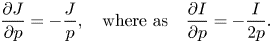 \begin{equation} \frac{\partial J}{\partial p}={-}\frac{J}{p}, \quad \textrm{where as} \quad \frac{\partial I}{\partial p}={-}\frac{I}{2p}. \end{equation}
Accounting for this difference, it is straightforward to modify (A3) so that the vCIDR equations are linearly well-posed if the following three conditions on the constitutive functions  $Y,f$ are satisfied:
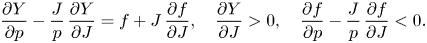 \begin{equation} \frac{\partial Y}{\partial p}-\frac{J}{p}\,\frac{\partial Y}{\partial J}=f+J\,\frac{\partial f}{\partial J}, \quad \frac{\partial Y}{\partial J}>0, \quad \frac{\partial f}{\partial p}-\frac Jp\,\frac{\partial f}{\partial J}<0. \end{equation}
 An additional benefit of the structure of the vCIDR equations is that, as discussed in Goddard & Lee (Reference Goddard and Lee2018) and Schaeffer et al. (Reference Schaeffer, Barker, Tsuji, Gremaud, Shearer and Gray2019), the well-posedness conditions (5.4) in turn guarantee Onsager symmetry and positive dissipation rates (as illustrated in Appendix B). These important thermodynamic implications are, however, not present in the alternative compressible formulation of Heyman et al. (Reference Heyman, Delannay, Tabuteau and Valance2017) in which the dissipative terms ( $\boldsymbol {\nabla } \boldsymbol {\cdot } \boldsymbol{\tau}$) are instead based upon the inclusion of a $\phi$-dependent volumetric viscosity.
5.1. Connection to $\mu (J), \varPhi (J)$ rheology

Many constitutive functions  $Y(p,\phi,J)$ and $f(p,\phi,J)$ satisfying (5.4) are possible. The PDE relating $Y$ and $f$ is independent of $\phi$, as are the inequality constraints. However, in choosing these functions, it is desirable to maintain consistency with $\mu (J), \varPhi (J)$ rheology in the case of isochoric deformations, for which $\phi =\varPhi (J)$ when $\boldsymbol {\nabla } \boldsymbol {\cdot }\boldsymbol {u}=0$. To accomplish this property, take
 \begin{equation} Y(p,\phi,J)=\mu(J)\,p \quad \mbox{and} \quad f(p,\phi,J)=0 \quad \mbox{if and only if}\quad J=\mathcal{J}(\phi), \end{equation}
where the function  $\mathcal {J}$ is the inverse of $\varPhi$, the strictly decreasing function in (2.14), which represents the viscous number for steady isochoric flow only.
One strategy for constructing suitable functions  $Y$ and $f$ is to first specify $Y(p,\phi,J)$ so that $Y(p,\varPhi (J),J)=\mu (J)p$ and $Y_J=\mu '(J)p>0$, and then construct $f(p,\phi,J)$ by solving the linear ordinary differential equation $Y_p-({J}/{p})Y_J=f+Jf_J$ for $f$ as a function of $J$, with the side condition from (5.5). This can be achieved by letting
 \begin{equation} Y(p,\phi,J)=\mu(\mathcal{J}(\phi))\,\frac{\alpha+(1-\alpha)J}{\alpha +(1-\alpha)\,\mathcal{J}(\phi)}\,p, \quad \mbox{with} \ 0<\alpha<1, \end{equation}
where  $\alpha$ is a new material parameter. Then
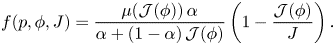 \begin{equation} f(p,\phi,J)=\frac{\mu(\mathcal{J}(\phi))\,\alpha}{\alpha+(1-\alpha)\, \mathcal{J}(\phi)}\left(1-\frac{\mathcal{J}(\phi)}{J}\right). \end{equation}
With these definitions, it is straightforward to check the conditions (5.4) and (5.5). In summary, with yield-stress and dilatancy specified by (5.6) and (5.7), the vCIDR rheology for suspensions is well-posed.
Equation (5.7) can be rearranged to isolate the viscous number  $J$:
$J$:
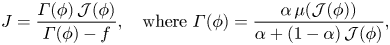 \begin{equation} J = \frac{\varGamma(\phi)\,\mathcal{J}(\phi)}{\varGamma(\phi)-f} , \quad \mbox{where} \ \varGamma(\phi)= \frac{\alpha\, \mu(\mathcal{J}(\phi))}{\alpha+(1-\alpha)\,\mathcal{J}(\phi)} , \end{equation}
and  $f=\boldsymbol {\nabla } \boldsymbol {\cdot }\boldsymbol {u}/(2\| {\boldsymbol{S}}\|)$ is used for brevity. From its general definition (2.9), the dynamic viscous number defines the pressure as
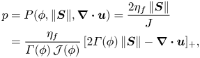 \begin{align} p &= P(\phi,\|{\boldsymbol{S}}\|,\boldsymbol{\nabla} \boldsymbol{\cdot}\boldsymbol{u}) = \frac{2\eta_f\,\|{\boldsymbol{S}}\|}{J} \nonumber\\ &=\frac{\eta_f}{\varGamma(\phi)\,\mathcal{J}(\phi)}\, [2\varGamma(\phi)\,\|{\boldsymbol{S}}\|-\boldsymbol{\nabla} \boldsymbol{\cdot}\boldsymbol{u}]_+ , \end{align}
where the notation  $[X]_+=\max (X,0)$ ensures that the pressure is non-negative, thus embodying the notion that the granular phase cannot sustain tension and that grains lose contact if the dilation is sufficiently fast compared to the shearing rate. When this equation of state for the pressure is substituted into the yield-stress function (5.6), the shear-stress tensor
 \begin{equation} {\boldsymbol{\tau}} = Y(P,\phi,J)\,\frac{{\boldsymbol{S}}}{\|{\boldsymbol{S}}\|}=2\eta_f \left\{\frac{[2\varGamma(\phi)\,\|{\boldsymbol{S}}\|-\boldsymbol{\nabla} \boldsymbol{\cdot}\boldsymbol{u}]_+}{2\,\mathcal{J}(\phi)\,\|{\boldsymbol{S}}\|}+ \frac{\varGamma(\phi)\,(1-\alpha)}{\alpha}\right\}{\boldsymbol{S}} \end{equation}
is formed, which can then be combined with the mass and momentum balance equations to generate a complete system of equations in terms of the natural kinematic variables  $\phi$ and spatial gradients of $\boldsymbol {u}$.
As a point of interest, the above formulation can be compared with the classical equations for compressible fluids. Following Chadwick (Reference Chadwick1976), the Cauchy stress tensor of the compressible Navier–Stokes equations may be written
 \begin{equation} \boldsymbol{\sigma}_{ij}=\{-\mathbb{P}+\zeta(\boldsymbol{\nabla} \boldsymbol{\cdot}\boldsymbol{u})\}\, \delta_{ij}+2\eta S_{ij} , \end{equation}
where  $\eta$ is the shear viscosity, $\zeta$ is the volumetric viscosity, and $\mathbb {P}$ is the thermodynamic pressure, each of which can depend on the fluid's local density and temperature (see e.g. Fine & Millero Reference Fine and Millero1973). For the vCIDR equations, the effective shear viscosity $\eta =Y/\| {\boldsymbol{S}}\|$ depends on both of the strain-rate invariants $\| {\boldsymbol{S}}\|$ and $\mathrm {tr}( {\boldsymbol{D}})=\boldsymbol {\nabla } \boldsymbol {\cdot }\boldsymbol {u}$, as well as the packing fraction, as detailed in (5.10). The equation of state of the effective thermodynamic pressure and the effective volumetric viscosity can then be found by comparing (5.11) with (5.9) to reveal that $\mathbb {P}$ depends here on $\| {\boldsymbol{S}}\|$ and $\phi$, whereas $\zeta$ depends only on $\phi$.
It is also illuminating to consider various limits of the vCIDR model. First, it is reassuring to confirm that for the special case of isochoric planar flow ( $\boldsymbol {\nabla } \boldsymbol {\cdot }\boldsymbol {u}=0$), (5.8) and (5.9) recover the Boyer et al. (Reference Boyer, Guazzelli and Pouliquen2011) relations $\| {\boldsymbol{\tau} }\|=\mu (\mathcal {J}(\phi ))\,p$ and $p=2\eta _f\,\| {\boldsymbol{S}}\|/\mathcal {J}(\phi )$. Then for volume-changing deformations, the new $\alpha$ parameter maps between distinct material responses: $\alpha =0$ corresponds to incompressibility, and $\alpha =1$ gives rate-independent behaviour. However, the incompressible limit cannot be reached since $\varGamma (\phi )\to 0$ as $\alpha \to 0$, from (5.8a), so that the pressure (5.9) in this limit is not well defined. This is to be expected as for truly incompressible flow, the pressure is either prescribed by external constraints or a response to the divergence-free velocity, rather than originating in the kinematics and packing of grains. In the other distinct limit, $\alpha \to 1$, the vCIDR relations approach a rate-independent bulk friction as $Y/p\to \mu (\mathcal {J}(\phi ))$, irrespective of the dilation rate, which leads to ill-posed dynamic equations. Consequently, both extreme values of $\alpha$ must be strictly omitted, therefore $\alpha =0.5$ will be used throughout the next section.
6. Numerical tests of vCIDR
Given the promising structure of the new vCIDR equations, in particular the guarantee of well-posedness, it is now important to explore their spatio-temporal solutions. As with the  $\mu (J),\varPhi (J)$ rheology in § 4 and the iCIDR equation in Schaeffer et al. (Reference Schaeffer, Barker, Tsuji, Gremaud, Shearer and Gray2019), here one-dimensional time-dependent solutions of flow in a shear cell are computed numerically using the MOL algorithm. The non-dimensional equations (4.2)–(4.4) are the same as in § 4. The key differences are that the non-dimensional pressure is given by
 \begin{equation} \tilde p =\frac{\tilde{\eta}_f}{\varGamma(\phi)\,\mathcal{J}(\phi)}\, [2\varGamma(\phi)\,\|\tilde{{\boldsymbol{S}}}\|-\tilde{\boldsymbol{\nabla}}\boldsymbol{\cdot}\tilde{\boldsymbol{u}}]_+, \end{equation}
and the non-dimensional shear-stress components are
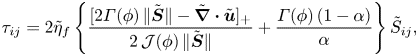 \begin{equation} \tau_{ij} =2\tilde{\eta}_f\left\{\frac{[2\varGamma(\phi)\,\| \tilde{{\boldsymbol{S}}}\|-\tilde{\boldsymbol{\nabla}}\boldsymbol{\cdot}\tilde{\boldsymbol{u}}]_+}{2\,\mathcal{J}(\phi)\,\| \tilde{{\boldsymbol{S}}}\|}+\frac{\varGamma(\phi)\,(1-\alpha)}{\alpha}\right\} \tilde{S}_{ij}, \end{equation}
instead of (4.5a,b) for the  $\mu (J),\varPhi (J)$ rheology.
The first test of vCIDR considers the same high-frequency modes (4.8) that were employed as initial data for the  $\mu (J),\varPhi (J)$ rheology in § 4. For both the low-packing fraction $\phi _0=0.35$ case and the high-packing fraction $\phi _0=0.55$ case, the solutions using vCIDR follow qualitatively the trend shown in figures 3(a,b). Specifically, the initial perturbation decays monotonically towards the uniform steady solution. Animations of these solutions can be found in supplementary movies 3 and 4, and the decay of the vertical velocity is tracked via the temporal evolution of its maximum value in figure 5.
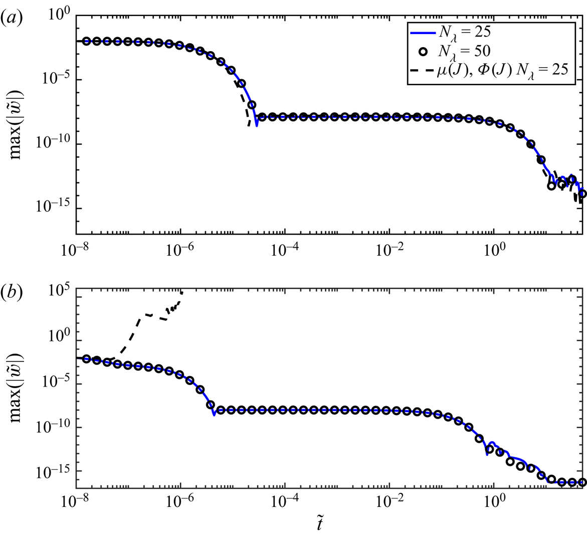
Figure 5. Temporal behaviour of the maximum amplitude of  $\tilde w$ for the vCIDR model given $\alpha =0.5$ and ${\tilde {\eta }_f =3.1}$. The initial conditions are identical to those in figures 3 and 4: (a) $\phi _0=0.35$, and (b) $\phi _0=0.55$. Here, two high-resolution cases are shown, with solid curves corresponding to $N_z=500$, and open circles to $N_z=1000$. Also reproduced, as dashed lines, are the equivalent high-resolution cases using the $\mu (J),\varPhi (J)$ rheology from figure 4.
Figure 5 also compares the vCIDR predictions directly with the equivalent behaviour of the  $\mu (J),\varPhi (J)$ rheology. The difference made by vCIDR is clear: whilst evolution is almost identical in the low $\phi _0$ case, the vCIDR solutions are grid converged and lead to long-time stability in the high $\phi _0$ case, unlike the grid-dependent blow-up observed when the $\mu (J),\varPhi (J)$ rheology is solved in the same setting. Whilst expected due to the well-posedness analysis, this difference in transient behaviour is both striking and suggests that the new model is a good candidate for the simulation of realistic inhomogeneous flows for which the volume fraction is likely to span a wide range of values.
It is also interesting to consider larger perturbations, away from the steady long-time solution, as initial data. Taking
 \begin{equation} \tilde u(\tilde z,\tilde t=0) = \tilde z , \quad \tilde w(\tilde z,\tilde t=0) = 0, \quad \phi(\tilde z,\tilde t=0) = \phi_{crit} + A\sin(2{\rm \pi}\tilde z), \end{equation}
means that the bottom half of the domain initially has  $\phi >\phi _{crit}$, whereas the top half has $\phi <\phi _{crit}$. These initial conditions therefore straddle the point of ill-posedness for the $\mu (J), \varPhi (J)$ rheology. The evolution away from this initial data, using vCIDR, is plotted in figure 6. As expected, the steady solution is recovered in the long-time limit, and there are no spurious oscillations found even when computing using a very fine resolution ( ${N_z=401}$) mesh. An animation of this solution can be found in supplementary movie 5.
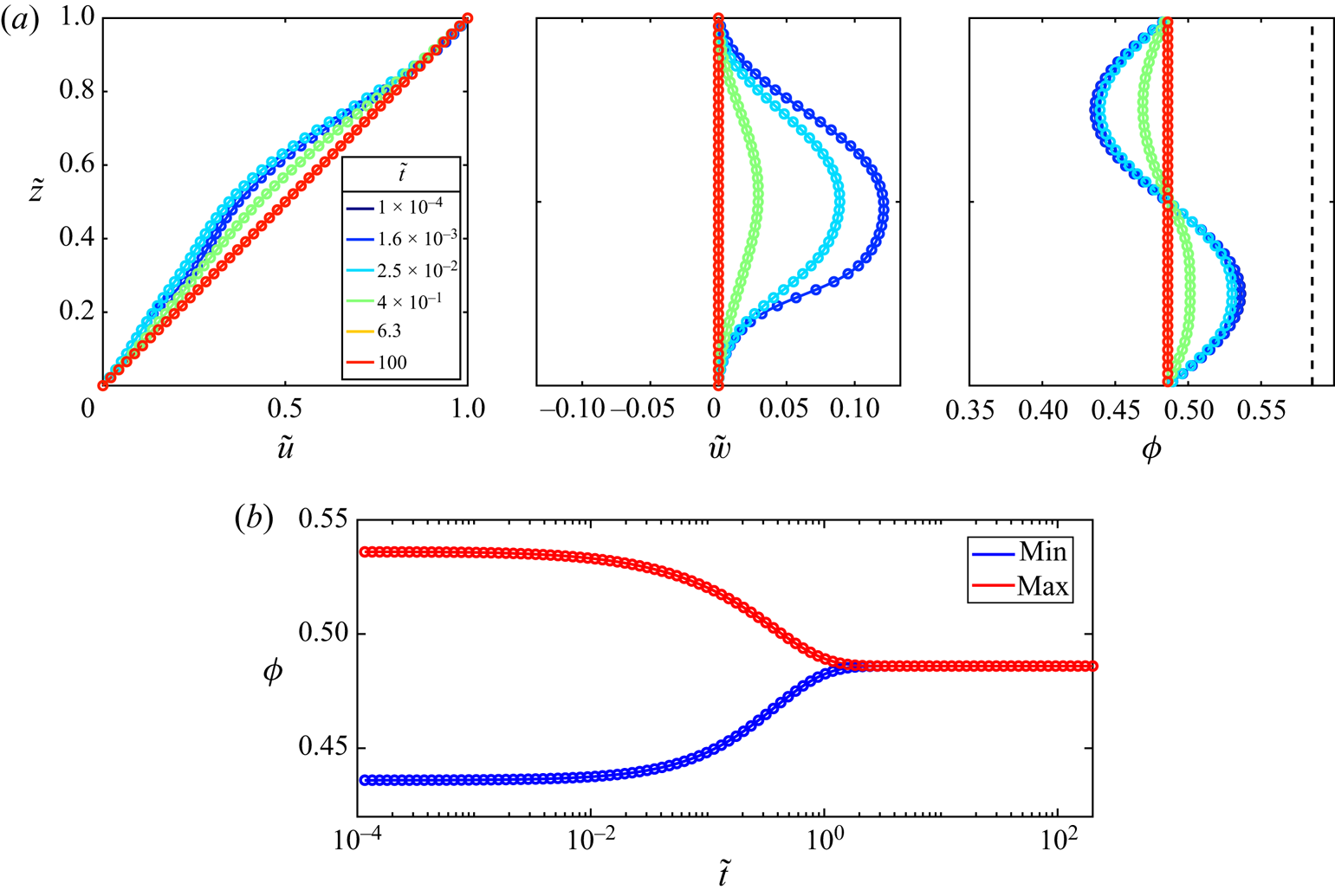
Figure 6. Evolution of the straddling initial data (6.3) with amplitude  $A=0.05$ for the vCIDR model with $\alpha =0.5$ and $\tilde {\eta }_f =3.1$. Panel (a) shows the flow fields plotted at different times, and (b) is the evolution of the minimum and maximum values of $\phi (\tilde z,\tilde t)$ in the domain. Solid lines are with $N_z=401$, and open circles are for $N_z=47$.
As a final numerical comparison, figure 7 plots the straddling simulation from figure 6 as a space–time colour map alongside an equivalent simulation using the  $\mu (J),\varPhi (J)$ rheology. As shown in figure 7(b), the $\mu (J),\varPhi (J)$ rheology code fails at an early time ( $\tilde t\approx 2\times 10^{-4}$) due to spontaneous instabilities that emerge in the ill-posed high-packing region at the bottom of the flow. In contrast, the vCIDR case shown in figure 7(a) exhibits a smooth homogenisation of the initially non-uniform mass. In addition to effectively demonstrating the connotations for numerical stability, in agreement with the analysis of §§ 3 and 5, these simulations provide impetus that the vCIDR model would be a preferred candidate for the simulation of other particle migration problems such as settling (Bang et al. Reference Bang, Lefrançois, Sergent and Bertrand2008) and transient channel flow (Lyon & Leal Reference Lyon and Leal1998), provided that a realistic drag model is also employed.
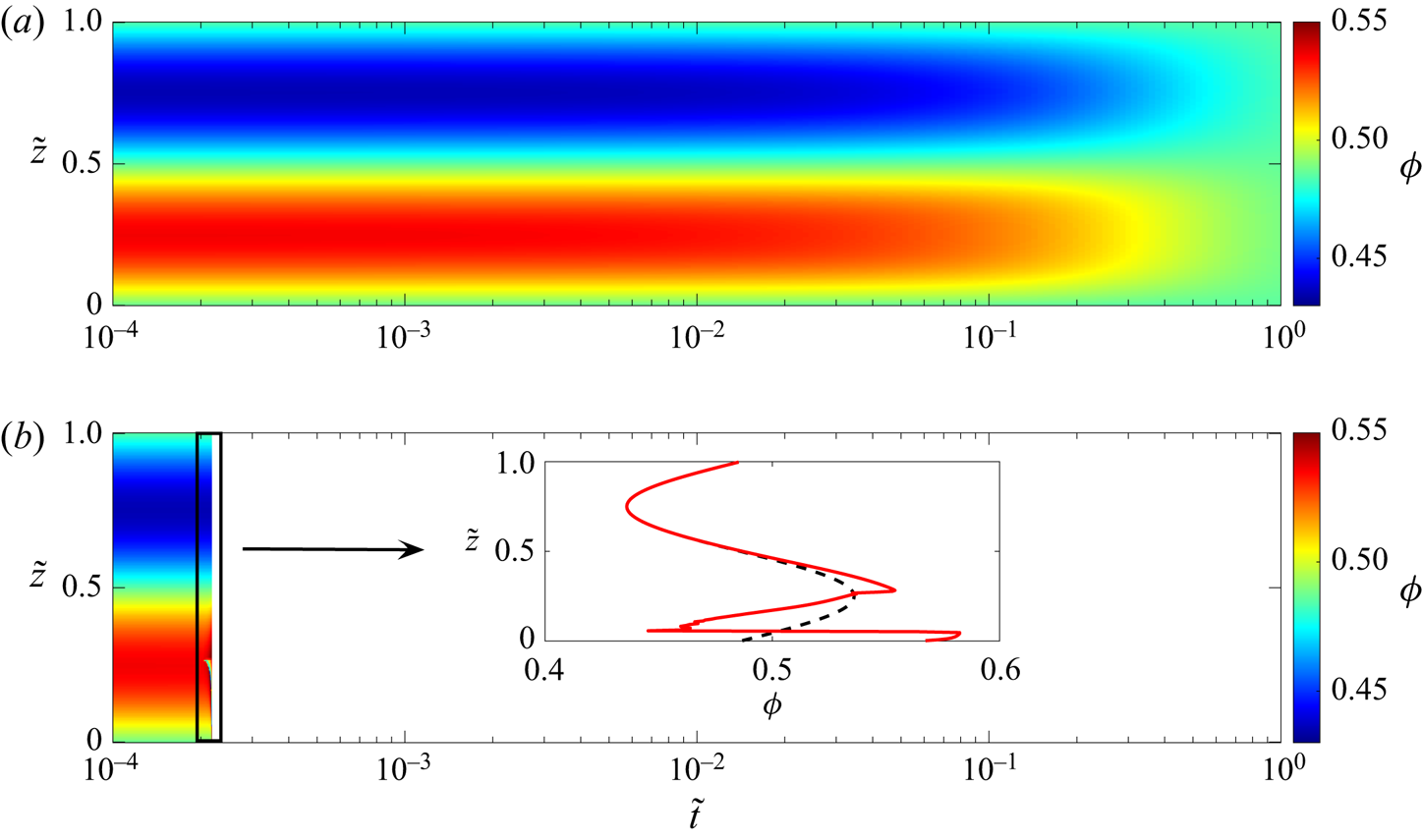
Figure 7. A space–time comparison, on a semi-logarithmic axis, of the solid volume fraction evolution from the straddling initial condition (6.3) with  $A=0.05$ for (a) the vCIDR model, and (b) the $\mu (J),\varPhi (J)$ rheology. Inset in (b) is the final solid volume fraction profile in the $\mu (J),\varPhi (J)$ rheology simulation before the failure of numerical convergence; the dashed curve in that plot is the initial $\phi$ profile. The vCIDR simulation uses $N_z=401$ spatial points, whereas the $\mu (J),\varPhi (J)$ rheology is performed with $N_z=201$. Animations of these cases can be found in supplementary movies 5 and 6.
7. Rheology spanning the viscous and inertial regimes
7.1. Formulation and general conditions for well-posedness of single-phase models depending on both $I$ and $J$


As described by Trulsson et al. (Reference Trulsson, Andreotti and Claudin2012), there is a smooth transition between flow dominated by  $I$-dependence and flow dominated by $J$-dependence. This happens because the particle Stokes number
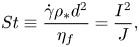 \begin{equation} St \equiv \frac{\dot{\gamma}\rho_*d^2}{\eta_f} = \frac{I^2}{J} , \end{equation}
which describes the ratio of inertial to viscous effects, varies with strain rate. At large values of  $\dot {\gamma }$, particle collisions become more important than hydrodynamic forces, and the rheology of the suspension is effectively that of dry material. Trulsson et al. (Reference Trulsson, Andreotti and Claudin2012) find a good collapse for steady homogeneous flows by taking
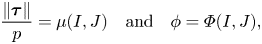 \begin{equation} \frac{\|{\boldsymbol{\tau}}\|}{p}=\mu(I,J) \quad \mbox{and} \quad \phi=\varPhi(I,J) , \end{equation}
i.e. a synthesis of the  $\mu (I),\varPhi (I)$ rheology of Pouliquen et al. (Reference Pouliquen, Cassar, Jop, Forterre and Nicolas2006) with the $\mu (J),\varPhi (J)$ rheology of Boyer et al. (Reference Boyer, Guazzelli and Pouliquen2011). Whilst it would be of interest to detail the well-posedness of this mixed rheology, § 3 of the present study and the work of Heyman et al. (Reference Heyman, Delannay, Tabuteau and Valance2017) already highlight severe deficiencies when either $I$- or $J$-dependence is negligible.
As a generalised synergy of both vCIDR and the previous  $I$-dependent version, take
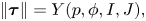 $$\begin{gather} \|{\boldsymbol{\tau}}\| = Y(p,\phi,I,J) , \end{gather}$$
 $$\begin{gather}\boldsymbol{\nabla} \boldsymbol{\cdot}\boldsymbol{u} = 2\|{\boldsymbol{S}}\,\| f(p,\phi,I,J) . \end{gather}$$
To ensure that this new rheology gives well-posed equations, the yield-stress function  $Y$ and dilatancy function $f$ should be chosen to satisfy
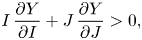 $$\begin{gather} I\,\frac{\partial Y}{\partial I}+J\,\frac{\partial Y}{\partial J}>0 , \end{gather}$$
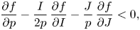 $$\begin{gather}\frac{\partial f}{\partial p}-\frac{I}{2p}\,\frac{\partial f}{\partial I}-\frac{J}{p}\,\frac{\partial f}{\partial J}<0 , \end{gather}$$
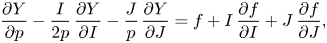 $$\begin{gather}\frac{\partial Y}{\partial p}-\frac{I}{2p}\,\frac{\partial Y}{\partial I}-\frac{J}{p}\,\frac{\partial Y}{\partial J} = f+I\,\frac{\partial f}{\partial I}+J\,\frac{\partial f}{\partial J}, \end{gather}$$
where the strain rate and pressure dependence of  $I$ and $J$ enter independently.
7.2. An ill-posed example motivated by the equations of Baumgarten & Kamrin (Reference Baumgarten and Kamrin2019)
Despite the extended system of constitutive functions (7.3) and their related well-posedness conditions (7.4) appearing cumbersome, recent models can easily be cast into this framework. For example, Baumgarten & Kamrin (Reference Baumgarten and Kamrin2019) propose
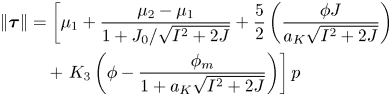 \begin{align} \|{\boldsymbol{\tau}}\| &= \left[ \mu_1 +\frac{\mu_2-\mu_1}{1+J_0/\sqrt{I^2+2J}}+ \frac{5}{2}\left(\frac{\phi J}{a_K\sqrt{I^2+2J}}\right) \right.\nonumber\\ & \quad + \left. K_3 \left(\phi-\frac{\phi_m}{1+a_K\sqrt{I^2+2J}}\right) \right] p \end{align}
and
 \begin{equation} p = \frac{(a_K\phi)^2}{(\phi_m-\phi)^2}\, [\rho_*d^2(2\|{\boldsymbol{S}}\|-K_4\,\boldsymbol{\nabla} \boldsymbol{\cdot}\boldsymbol{u})^2+2\eta_f(2\|{\boldsymbol{S}}\|-K_4\,\boldsymbol{\nabla} \boldsymbol{\cdot}\boldsymbol{u})] , \end{equation}
where  $a_K$, $K_3$ and $K_4$ are constant material parameters. Incidentally, this formulation is closely related to the proposed model of Trulsson et al. (Reference Trulsson, Andreotti and Claudin2012) when value $\alpha _K=1/2$ is taken in their combined viscous–inertial number $\mathcal {K}=J+\alpha _K I^2$. Comparison of these particle-phase relations with (7.3) is aided as the yield-stress function (7.5) is already in the form of (7.3a), whereas (7.6) must be rearranged into the form of a CIDR dilatancy rule. Dividing both sides of (7.6) by $p$ and collecting terms gives
 \begin{equation} I^2(1-K_4f)^2+2J(1-K_4f)=A(\phi) , \end{equation}
where  $f=\boldsymbol {\nabla } \boldsymbol {\cdot }\boldsymbol {u}/(2\| {\boldsymbol{S}}\|)$ and
 \begin{equation} A(\phi)=\frac{(\phi_m-\phi)^2}{(a_K\phi)^2} . \end{equation}
Solving the quadratic equation (7.7) for  $f$ and taking the most compressive branch (to which Baumgarten & Kamrin (Reference Baumgarten and Kamrin2019) limit attention) then gives
 \begin{equation} f(p,\phi,I,J)=\frac{I^2+J-\sqrt{A(\phi)\,I^2+J^2}}{K_4I^2} . \end{equation}
This form satisfies (7.4b) for all  $K_4>0$, and similarly (7.5) satisfies (7.4a) for typical parameter values because all terms are increasing functions of $I$ and $J$. However, these specific choices do not satisfy the well-posedness consistency condition (7.4c). The right-hand side is conveniently equal to $1/K_4$, which clearly is not matched by the left-hand side as (7.5) is not of a complementary form.
It is important to note that the above analysis does not constitute a proof of ill-posedness for the full equations of Baumgarten & Kamrin (Reference Baumgarten and Kamrin2019). In that work, the effective suspension rheology is coupled to a much larger system of equations that model many additional physical processes. Notably, Baumgarten & Kamrin (Reference Baumgarten and Kamrin2019) present a two-fluid framework that incorporates explicit coupling to the background liquid motion, including pore pressure effects, and elasticity to accommodate material below yield. Despite none of these extensions currently being accommodated by CIDR, the above example still highlights the pitfalls of constitutive modelling without consideration of well-posedness.
7.3. A well-posed example: viCIDR
Noting that the pressure equation (7.6) recovers the correct inertial scaling  $p\propto \| {\boldsymbol{S}}\|^2$ as $\eta _f\to 0$, and the correct viscous scaling $p\propto \| {\boldsymbol{S}}\|$ as $St\to 0$, inspires us to take a similar form as the starting point and then derive a complementary yield-stress function to replace (7.5) in order to guarantee well-posedness. The primary modification made here to (7.6) is to allow for different $\phi$ dependence in the dry limit ( $\eta _f\to 0$) than in the viscous limit ( $St\to 0$).
The pressure is constructed as the additive combination of dry and viscous pressures such that
 \begin{align} p &= P(\phi,\|{\boldsymbol{S}}\|,\boldsymbol{\nabla} \boldsymbol{\cdot}\boldsymbol{u}) \nonumber\\ &= \frac{\rho_*d^2}{\mathcal{I}(\phi)^2}\, [2\|{\boldsymbol{S}}\|-K\,\boldsymbol{\nabla} \boldsymbol{\cdot}\boldsymbol{u}]_+^2+ \frac{\eta_f}{\mathcal{J}(\phi)}\, [2\|{\boldsymbol{S}}\|-K\,\boldsymbol{\nabla} \boldsymbol{\cdot}\boldsymbol{u}]_+ , \end{align}
where  $K$ is a constant compressibility factor. For isochoric flows ( $\boldsymbol {\nabla } \boldsymbol {\cdot }\boldsymbol {u}=0$), this form can be made compatible with the particle simulations of Trulsson et al. (Reference Trulsson, Andreotti and Claudin2012) and the recent experimental work of Tapia et al. (Reference Tapia, Ichihara, Pouliquen and Guazzelli2022) by taking
 \begin{equation} \mathcal{J}(\phi)=\left(\frac{\phi_c-\phi}{a_\phi}\right)^2 \quad \mbox{and} \quad \mathcal{I}(\phi)= \frac{\phi_c-\phi}{a_\phi\sqrt{\alpha_\phi}}, \end{equation}
where the material constants  $a_\phi$ and $\alpha _\phi$ follow the notation of Tapia et al. (Reference Tapia, Ichihara, Pouliquen and Guazzelli2022) and work to scale the relative contributions of the inertial and viscous dynamics. It is also pleasing to note that the $\varPhi (I)$ rheology for dry granular flow is recovered precisely in the absence of a background fluid ( $\eta _f=0$). This feature would be vital for modelling complex non-uniform flows with both saturated and dry regions, as is often the case in debris avalanches (see Meng, Johnson & Gray Reference Meng, Johnson and Gray2022).
This formulation is also assisted by the calculation, similar to that in § 7.2, that the second well-posedness inequality (7.4b) is automatically satisfied for  $K>0$, and that the right-hand side of the well-posedness equality (7.4c) is simply equal to $1/K$. As in (7.5), here $Y$ is constructed from the product of $p$ and a general bulk friction $\mu$ such that
 \begin{equation} Y(p,\phi,I,J) = \mu(\phi,I,J)\,p , \end{equation}
which also shares similarity with the vCIDR model (5.6) and the iCIDR equations of Schaeffer et al. (Reference Schaeffer, Barker, Tsuji, Gremaud, Shearer and Gray2019). As such, this new model will be denoted ‘viCIDR’ to highlight the inclusion of both viscous and inertial regimes.
Limiting attention to homogeneous solutions of (7.4c) reveals that
 \begin{equation} \mu(\phi,I,J) = \mu_1+B(\phi)\,I^2+C(\phi)\,J , \end{equation}
where  $B$ and $C$ are free functions of $\phi$, satisfies all of the well-posedness conditions (7.4) provided that
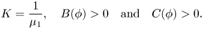 \begin{equation} K = \frac{1}{\mu_1} , \quad B(\phi)>0 \quad \mbox{and} \quad C(\phi)>0 . \end{equation}
These forms are also shown to have non-negative dissipation rates in Appendix B. The remaining closures come from matching the  $J=0$ limit with the steady isochoric ( $\boldsymbol {\nabla } \boldsymbol {\cdot }\boldsymbol {u}=0$) dry granular rheology of Jop et al. (Reference Jop, Forterre and Pouliquen2006):
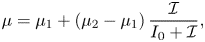 \begin{equation} \mu=\mu_1+(\mu_2-\mu_1)\,\frac{\mathcal{I}}{I_0+\mathcal{I}}, \end{equation}
where  $I_0$ and $\mu _2$ are rheological constants mediating the transition to dynamic flow, and matching with the Boyer et al. (Reference Boyer, Guazzelli and Pouliquen2011) form of $\mu$ (2.10) for $I=0$. However, these choices are simply demonstrative rather than adhering to any further empirical results. This procedure gives
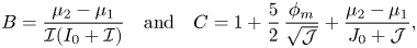 \begin{equation} B=\frac{\mu_2-\mu_1}{\mathcal{I}(I_0+\mathcal{I})} \quad \mbox{and} \quad C=1+\frac{5}{2}\,\frac{\phi_m}{\sqrt{\mathcal{J}}}+\frac{\mu_2-\mu_1}{J_0+\mathcal{J}}, \end{equation}
so that the bulk friction is
 \begin{align} \mu(I,J,\phi) = \mu_1+(\mu_2-\mu_1)\left[\frac{I}{I_0+\mathcal{I}(\phi)}\, \frac{I}{\mathcal{I}(\phi)}+\frac{J}{J_0+\mathcal{J}(\phi)}\right]+J+ \frac{5}{2}\,\phi_m\,\frac{J}{\sqrt{\mathcal{J}(\phi)}}. \end{align}
8. Conclusions and discussion
In this paper, the single-phase model for flowing suspensions of Boyer et al. (Reference Boyer, Guazzelli and Pouliquen2011), known as the  $\mu (J),\varPhi (J)$ rheology, has been shown to give well-posed evolution equations only for low solid volume fractions $\phi <\phi _{crit}$, and otherwise leads to ill-posed equations for all flows at higher concentrations, as summarised graphically in figure 1. This finding therefore strongly limits the applicability of the $\mu (J),\varPhi (J)$ rheology in numerical calculations of complex time-varying flows of suspensions.
An alternative theory named vCIDR, in which  $\phi$ is a fully independent variable, has been introduced, along with conditions which, when satisfied, guarantee well-posedness in all flow regimes, at any solid concentration. A specific choice for the functions in vCIDR has been made here to illustrate the regularisation that this framework enables and to show how the well-established $\mu (J)$ and $\varPhi (J)$ relations may be included for steady isochoric deformations. Numerical computations of perturbations to shear flow have then been used to verify the predicted difference in dynamics between the formulations. Since the framework of vCIDR has been verified both theoretically and numerically to give robust predictions of dynamic deformations, the theory can now be tested against suitable experiments. In particular, the precise form of the vCIDR constitutive relations will depend on the results of prototype experiments and discrete particle simulations designed to test transient deformations.
Whilst vCIDR represents a complete mathematical theory for suspensions, it is based on the approximations inherent in the single-phase effective medium hypothesis. The equations track the particle-phase dynamics assuming that the background fluid does not evolve in response to this motion, simply mediating hydrodynamics and drag on the particles. These approximations are employed directly in the particle simulations of Trulsson et al. (Reference Trulsson, Andreotti and Claudin2012) and Ness & Sun (Reference Ness and Sun2016), who have reproduced the steady Boyer et al. (Reference Boyer, Guazzelli and Pouliquen2011) without an explicit background fluid. It remains to be seen, however, whether regimes exist in which transient flows are similarly matched between these simulations, physical experiments and vCIDR.
For regimes in which truly de-coupled motion of both fluid and particles is necessary, one must instead turn to the alternative two-fluid description (see e.g. Guazzelli & Pouliquen Reference Guazzelli and Pouliquen2018; Baumgarten & Kamrin Reference Baumgarten and Kamrin2019). Such an approach is more realistic, yet naturally more complex and requires many further constitutive relations to be chosen, the forms of which are subject to much debate (see Nott, Guazzelli & Pouliquen (Reference Nott, Guazzelli and Pouliquen2011) for a discussion). Moreover, an understanding of the well-posedness of equations for two-phase phase suspension flow is currently lacking. Because vCIDR includes many of the key features required of such a theory – well-posedness, Onsager symmetry and a non-negative dissipation rate – it is hoped that the constitutive relations proposed in this paper can aid future model development.
As the formulation of vCIDR in § 5 includes dependence on only the viscous number  $J$ and not the inertial number $I$, the theory is technically limited to slow flows for which the inertial rearrangement of grains is negligible. Maurin, Chauchat & Frey (Reference Maurin, Chauchat and Frey2016) have instead shown that for relatively fast flows, such as those of importance in bedload transport, the particle dynamics is well approximated by $I$-dependent models, without inclusion of the viscous number. The transition between these distinct scalings, in terms of strain rate and pressure, is the topic of Trulsson et al. (Reference Trulsson, Andreotti and Claudin2012). These findings are addressed here through the viCIDR model, introduced in § 7.3, which is an augmentation of vCIDR spanning both the viscous and inertial regimes.
In addition to the extensions to two-phase flow and multiple regimes, there are other dynamic variables that may be important in a full continuum description of suspensions. For example, Wyart & Cates (Reference Wyart and Cates2014) and Gillissen et al. (Reference Gillissen, Ness, Peterson, Wilson and Cates2019) provide frameworks for tracking the evolving networks of contact between grains, the details of which are thought to be vital to describing the jamming transition and hysteretic effects. Coupling vCIDR to these equations would take the structure of the equations outside the scope of the present work, but the implications for well-posedness are worth exploring.
Supplementary movies
Supplementary movies are available at https://doi.org/10.1017/jfm.2022.1004.
Funding
T.B. was supported in this work by NERC grant NE/W004240/1. J.M.N.T.G. was supported by an EPSRC Established Career Fellowship (EP/M022447/1), a Royal Society Wolfson Research Merit Award (WM150058) and NERC grant NE/X00029X/1. M.S. was supported by National Science Foundation grant DMS-1812445. An LMS Scheme 2 grant and a Heilbronn Institute small grant also enabled the collaboration of T.B. and D.G.S.
Declaration of interests
The authors report no conflict of interest.
Appendix A. Well-posedness analysis for the compressible $I$-dependent rheology (CIDR)

The CIDR equations of Barker et al. (Reference Barker, Schaeffer, Shearer and Gray2017) were formulated for dry granular materials as a rate-dependent extension to classical critical-state soil mechanics. In the absence of a background fluid, the important non-dimensional strain rate is the inertial number  $I$ as defined in (2.8). CIDR was then formulated in terms of a yield-stress function $Y$ such that
 \begin{equation} \|\boldsymbol{\tau}\|=Y(p,\phi,I) , \end{equation}
and a dilatancy function  $f$ that sets
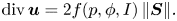 \begin{equation} \mbox{div} \, \boldsymbol{u}=2f(p,\phi,I)\,\| \boldsymbol{S}\|. \end{equation}
Similarly to the analysis presented here in § 3, the well-posedness of the CIDR equations was ascertained via a linear stability analysis carried out in the high wavenumber limit. The leading-order eigenvalue problem sets three conditions under which the growth rates of high-frequency modes are negative. In particular,  $Y$ and $f$ must be chosen to satisfy
 \begin{equation} \frac{\partial I}{\partial \|{\boldsymbol{S}}\|}\,\frac{\partial Y}{\partial I}>0 , \quad \frac{\partial f}{\partial p}+\frac{\partial I}{\partial p}\,\frac{\partial f}{\partial I}<0 \quad \mbox{and} \quad \frac{\partial Y}{\partial p}+\frac{\partial I}{\partial p}\,\frac{\partial Y}{\partial I} = f+I\,\frac{\partial f}{\partial I} , \end{equation}
where the inertial number dependence gives
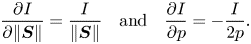 \begin{equation} \frac{\partial I}{\partial \|{\boldsymbol{S}}\|}=\frac{I}{\|{\boldsymbol{S}}\|} \quad \mbox{and} \quad \frac{\partial I}{\partial p}={-}\frac{I}{2p} . \end{equation}
Not only do these relations ensure important mathematical and numerical properties of the equations, but Goddard & Lee (Reference Goddard and Lee2018) and Schaeffer et al. (Reference Schaeffer, Barker, Tsuji, Gremaud, Shearer and Gray2019) have shown that these criteria embody the key thermodynamic principle of Onsager symmetry.
Appendix B. Non-negative dissipation rates of vCIDR and viCIDR
In addition to Onsager symmetry, which is a feature inherent in all CIDR models, it is also important to establish that the proposed constitutive relations lead to non-negative dissipation rates
 \begin{equation} \mathcal{D} = {\boldsymbol{\sigma}} : {\boldsymbol{D}} \geq 0 , \end{equation}
i.e. that deformations do not correspond to negative work done. For each CIDR theory, the dissipation rate may be calculated via
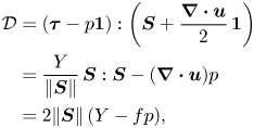 \begin{align} \mathcal{D} &= ({\boldsymbol{\tau}}-p{\boldsymbol{1}}):\left({\boldsymbol{S}}+\frac{\boldsymbol{\nabla} \boldsymbol{\cdot}\boldsymbol{u}}{2}\,{\boldsymbol{1}}\right)\nonumber\\ &=\frac{Y}{\|{\boldsymbol{S}}\|}\,{\boldsymbol{S}}:{\boldsymbol{S}}-(\boldsymbol{\nabla} \boldsymbol{\cdot}\boldsymbol{u})p \nonumber\\ &= 2\|{\boldsymbol{S}}\|\,(Y-fp) , \end{align}
due to the general definitions of the constitutive laws and of the norm (cf. (2.6))
 \begin{equation} \|{\boldsymbol{S}}\|=\sqrt{\tfrac{1}{2}{\boldsymbol{S}}:{\boldsymbol{S}}} . \end{equation}
B.1. vCIDR dissipation rate
For the vCIDR constitutive functions (5.9) and (5.10), the dissipation rate (B2) is
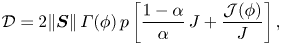 \begin{equation} \mathcal{D}=2\|{\boldsymbol{S}}\|\,\varGamma(\phi)\,p \left[\frac{1-\alpha}{\alpha}\,J+\frac{\mathcal{J}(\phi)}{J}\right] , \end{equation}
which is non-negative as  $p$,
$p$,  $\| {\boldsymbol{S}}\|$ and $\varGamma (\phi )$ are non-negative and $0<\alpha <1$.
It is also important to rule out unbounded dissipation, which could occur in (B4) for  $J\to 0$. However, combining (5.8a) and (5.9) reveals that the potentially problematic term, which scales with
 \begin{equation} \frac{p}{J}=\frac{2\eta_f\,\|{\boldsymbol{S}}\|}{J^2}= \frac{2\eta_f\,\|{\boldsymbol{S}}\|}{(\varGamma(\phi)\, \mathcal{J}(\phi))^2}\,(\varGamma(\phi)-f)^2, \end{equation}
is well-behaved for all finite values of shear strain rate and compression. In conclusion, (B4) is non-negative and finite for all flows in the viscous range ( $\phi <\phi _m$).
B.2. viCIDR dissipation rate
Upon substituting the general viscous–inertial functions (7.12) and (7.13) into (B2) one arrives at
 \begin{equation} \mathcal{D} = 2\|{\boldsymbol{S}}\|\,(\mu_1 P+4d^2\rho_*\, B(\phi)\,\|{\boldsymbol{S}}\|^2+\eta_f\,C(\phi)\,\|{\boldsymbol{S}}\|)-(\boldsymbol{\nabla} \boldsymbol{\cdot}\boldsymbol{u}) P. \end{equation}
For this case, the establishment of non-negative  $\mathcal {D}$ rests on
 \begin{equation} (2\mu_1\,\|{\boldsymbol{S}}\|-\boldsymbol{\nabla} \boldsymbol{\cdot}\boldsymbol{u})P\geq 0. \end{equation}
Because  $K=1/\mu _1$ for well-posedness (7.14), cases in which the round brackets in (B7) are negative correspond to cases in which $P=0$ by (7.10). This ensures that (B7) is always satisfied and therefore that (B6) is always non-negative.


 Open access