


1. Introduction
Multiphase flows are common and a central topic in fluid mechanics (Prosperetti & Tryggvason Reference Prosperetti and Tryggvason2009), as they are present in a number of phenomena including pollutant dispersion, sedimentation, bubble spray in ocean dynamics as well as bubble columns.
Among the various kinds of multiphase flows, bubbly flows are a particularly challenging and key field of investigation, both for their fundamental dynamics and their numerous applications in engineering and environmental science (Magnaudet & Eames Reference Magnaudet and Eames2000; Prosperetti Reference Prosperetti2004; Clift, Grace & Weber Reference Clift, Grace and Weber2005; Ern et al. Reference Ern, Risso, Fabre and Magnaudet2012; Lohse Reference Lohse2018; Mathai, Lohse & Sun Reference Mathai, Lohse and Sun2020). While much attention has been paid in the last decades to the dynamics of small inertial or neutrally buoyant particles (Crowe, Troutt & Chung Reference Crowe, Troutt and Chung1996; Balachandar & Eaton Reference Balachandar and Eaton2010; Maxey Reference Maxey2017; Elghobashi Reference Elghobashi2019), much less is known for bubbles, because they are experimentally, numerically and theoretically more complex (Prosperetti Reference Prosperetti2017; Mathai et al. Reference Mathai, Lohse and Sun2020).
In general, turbulent bubbly flows involve several complex and coupled physical mechanisms (Risso Reference Risso2018; Mathai et al. Reference Mathai, Lohse and Sun2020). In the absence of other external driving forces, buoyancy is the main source of motion: bubbles are much lighter than the surrounding fluid, and they rise attaining a significant velocity. This movement disturbs the carrying fluid inducing a collective agitation, referred to as pseudo-turbulence, bubble-induced turbulence or bubble-induced agitation. In turn, this induced agitation may affect the dynamics of the bubbles. Bubble-induced agitation is, therefore, one of the basic elements of bubbly flows and needs to be fully understood before being able to grasp more complex situations as well as proposing adequate models (Besagni, Inzoli & Ziegenhein Reference Besagni, Inzoli and Ziegenhein2018; Du Cluzeau, Bois & Toutant Reference Du Cluzeau, Bois and Toutant2019; Magolan, Lubchenko & Baglietto Reference Magolan, Lubchenko and Baglietto2019; Chahed & Masbernat Reference Chahed and Masbernat2020).
We focus in this work on this phenomenon, leaving out for the moment the presence of other effects such as the surrounding background turbulence, and also the detailed bubble dynamics. Moreover, we consider as the main test case a bubble column without walls, which is a common configuration in chemical engineering (Kantarci, Borak & Ulgen Reference Kantarci, Borak and Ulgen2005), and appears particularly suitable for the study of the physics of pseudo-turbulence.
Several experimental studies have been carried out to investigate this particular regime in different configurations (Lance & Bataille Reference Lance and Bataille1991; Zenit, Koch & Sangani Reference Zenit, Koch and Sangani2001; Martínez-Mercado, Palacios-Morales & Zenit Reference Martínez-Mercado, Palacios-Morales and Zenit2007; Riboux, Risso & Legendre Reference Riboux, Risso and Legendre2010; Mendez-Diaz et al. Reference Mendez-Diaz, Serrano-Garcia, Zenit and Hernandez-Cordero2013; Colombet et al. Reference Colombet, Legendre, Risso, Cockx and Guiraud2015), and significant progress has been made in figuring out the characteristic features of bubble-induced agitation (Risso Reference Risso2018). In particular, there is experimental evidence (Risso & Ellingsen Reference Risso and Ellingsen2002) that at moderate-to-large Reynolds numbers ( $Re>rsim 100$) the wakes of interacting bubbles are screened, which tends to show that at large Reynolds numbers the dominant mechanism underlying liquid agitation is the nonlinear wake interactions. Focusing on the liquid fluctuations induced by the bubbles, the key observations are that (i) the probability density function (p.d.f.) of the vertical fluctuations is strongly skewed while the horizontal one is symmetric, and both are non-Gaussian; (ii) the energy spectrum of the liquid agitation $E(k)$ displays a robust scaling, $E\sim k^{-3}$.
Some issues remain unclear, however. The range where this scaling applies is under discussion, with some experiments pointing to larger scales than the diameter (Riboux et al. Reference Riboux, Risso and Legendre2010), while others at smaller scales (Mercado et al. Reference Mercado, Gomez, Van Gils, Sun and Lohse2010; Prakash et al. Reference Prakash, Mercado, van Wijngaarden, Mancilla, Tagawa, Lohse and Sun2016). Moreover, in some experiments a Kolmogorov spectrum  $E\sim k^{-5/3}$ might be present at small (Martínez-Mercado et al. Reference Martínez-Mercado, Palacios-Morales and Zenit2007; Riboux et al. Reference Riboux, Risso and Legendre2010) or at large scales (Prakash et al. Reference Prakash, Mercado, van Wijngaarden, Mancilla, Tagawa, Lohse and Sun2016). From a physical point of view, two main mechanisms appear to underlie these scalings: the superposition of Gaussian fluctuations generated near the bubbles (Risso Reference Risso2011) because of the disordered bubble distribution; and the turbulent fragmentation (Lance & Bataille Reference Lance and Bataille1991) notably at high Reynolds number. It is difficult to disentangle these two mechanisms, as the steep spectrum $E\sim k^{-3}$ corresponds to a smooth flow (Monin & Yaglom Reference Monin and Yaglom1975), which may be related to a number of different situations (Boffetta & Ecke Reference Boffetta and Ecke2012). The relation between pseudo-turbulence and turbulence is also linked to the last issue. In particular, fluid turbulence is mainly characterised by a cascade phenomenon, expressed by a constant flux of kinetic energy towards a certain range of scales (Frisch Reference Frisch1995; Boffetta & Ecke Reference Boffetta and Ecke2012; Alexakis & Biferale Reference Alexakis and Biferale2018). The existence of such a cascade in the pseudo-turbulence regime would help to understand the underlying mechanisms. Because the injection of energy is made via buoyancy, it is not clear a priori which scales are forced and towards which scales the energy is transferred. It remains, therefore, to be addressed if: (a) there is an energy cascade and in what direction; (b) whether the shape of the spectrum and then the underlying mechanisms may be traced back to the energy cascade; (c) whether the Reynolds number has any influence on the results.
The aim of this work is to address these issues with high-resolution numerical simulations, combining several two-dimensional (2-D) and three-dimensional (3-D) numerical experiments.
Indeed, experiments have the great advantage of easily dealing with large  $Re$ number flows. Nevertheless, the experimental investigation of turbulent bubbly flows is difficult, and isolating and analysing the bubble-induced agitation is tricky (Risso Reference Risso2018). For instance, the p.d.f. of the amplitude of the velocity was measured by Martínez-Mercado et al. (Reference Martínez-Mercado, Palacios-Morales and Zenit2007), yet the p.d.f. of the vertical and horizontal components of the velocity have been so far measured only by Riboux et al. (Reference Riboux, Risso and Legendre2010) and by Bouche et al. (Reference Bouche, Roig, Risso and Billet2014) in a thin gap. Furthermore, boundary and impurity effects may be present, and getting information about small scales and energy-flux statistics is practically impossible.
For these reasons, numerical simulations have appeared early as a necessary complementary tool both for homogeneous and bounded flows (Bunner & Tryggvason Reference Bunner and Tryggvason1999; Tryggvason et al. Reference Tryggvason, Bunner, Esmaeeli, Juric, Al-Rawahi, Tauber, Han, Nas and Jan2001; Fuster et al. Reference Fuster, Agbaglah, Josserand, Popinet and Zaleski2009; Dabiri, Lu & Tryggvason Reference Dabiri, Lu and Tryggvason2013; Dabiri & Tryggvason Reference Dabiri and Tryggvason2015; Elghobashi Reference Elghobashi2019). However, the numerical approach has its own limitations. Numerical experiments supposed to reproduce actual experiments must be designed so as to resolve all the characteristic time scales and spatial scales of the flow. The simulations fulfilling these criteria are called direct numerical simulations (DNS) of a flow, and are actually experiments in silico. The numerical investigation of bubble-induced agitation was pioneered by Bunner & Tryggvason (Reference Bunner and Tryggvason2002), who presented the first DNS of homogeneous free-array of bubbles, yet at low  $Re$ number ( $Re\approx 30$) and density ratio (approximately 50).
It is important to consider the interplay between numerics and physics to give the full context of the present work. Turbulent bubbly flows display a strong multiscale character with a very broad spectrum of scales, including the excited fluid modes (Pope Reference Pope2000) and the scales related to bubble boundary layers (Tryggvason, Scardovelli & Zaleski Reference Tryggvason, Scardovelli and Zaleski2011). In addition the density ratio between the two phases is generally very high (approximately  $1000$ in experimental flows) making the problem stiff. These numerical constraints come directly from the challenging physics of high Reynolds bubbly flows. A few attempts have been recently made to investigate pseudo-turbulence at high $Re$ number, notably with a similar purpose as here (Roghair et al. Reference Roghair, Mercado, Annaland, Kuipers, Sun and Lohse2011; Pandey, Ramadugu & Perlekar Reference Pandey, Ramadugu and Perlekar2020). In these studies the resolution has been kept at approximately 20 points per diameter ( ${\rm \Delta} x=d_b/20$), independently from the Reynolds number of the bubbles which is larger than 200 in most of the cases. This choice is related to studies carried out at low $Re$ number (Bunner & Tryggvason Reference Bunner and Tryggvason2002). A very recent study characterising the topological properties of the agitation induced by two bubbles (Hasslberger et al. Reference Hasslberger, Cifani, Chakraborty and Klein2020) is also worth mentioning. This work uses a higher resolution ( ${\rm \Delta} x=d_b/40$), but for a flow at very high Reynolds number, larger than $900$. However, Cano-Lozano et al. (Reference Cano-Lozano, Martinez-Bazan, Magnaudet and Tchoufag2016a) have shown that such a resolution does not allow us to properly resolve the boundary layers around bubbles at high Reynolds number and this may lead to quantitative and even qualitative errors on the dynamics. The resolution should rather increase proportionally to the bubble Reynolds number. From a more quantitative point of view, let us recall that around bubbles a thin boundary layer develops, whose thickness scales like $\delta \sim Re^{-1/2}$ (Moore Reference Moore1963; Landau & Lifshitz Reference Landau and Lifshitz1987). That means that a resolution of $d_b/{\rm \Delta} x\approx 20$ leads to less than one grid point in the boundary layer for $Re>100$.
Furthermore, in the first work (Roghair et al. Reference Roghair, Mercado, Annaland, Kuipers, Sun and Lohse2011) realistic physical properties are chosen but just a few bubbles are released, of the order of  $10$, while in the study by Pandey et al. (Reference Pandey, Ramadugu and Perlekar2020) many bubbles are followed but with a very low density ratio between the fluid and the gas, between 1.1 and 20. The nonlinear interactions among bubbles are, however, key to the dynamics and their statistical study requires the presence of a large number of bubbles (Lance & Bataille Reference Lance and Bataille1991; Risso Reference Risso2018). Moreover, while in some cases and with respect to specific observables the correct physics may be reproduced with a low density ratio (Diotallevi et al. Reference Diotallevi, Biferale, Chibbaro, Lamura, Pontrelli, Sbragaglia, Succi and Toschi2009), that cannot be claimed in general and requires further scrutiny.
As a matter of fact, these numerical simulations are implicitly coarse grained and, therefore, they should be considered as large eddy simulations (LES) rather than DNS. Without in any way diminishing their relevance, as for LES of single-phase flows, results may well be in accordance with experiments but comparison with resolved DNS appears necessary (Pope Reference Pope2000).
The purposes of the present study is, therefore, threefold. (i) To complement the few experimental results about pseudo-turbulence with a high-resolution DNS. (ii) To provide a reference fully resolved numerical experiment to analyse the effect of resolution in the different regimes. In particular, by direct comparison we want to assess to what extent coarser simulations are reliable. (iii) To exploit the detailed information available to a DNS, to help with understanding the physical mechanisms underlying the agitation, with particular attention paid to the possible cascade process. This uses in particular a scale-by-scale analysis to be described shortly.
The detailed contents of this paper are the following. In § 2 we review the basic mathematical framework of the problem, with particular attention paid to the different non-dimensional parameters relevant for the physics of bubbly flows. In § 3, we briefly introduce the numerical procedure. From a numerical point of view, different techniques can be used to study interfacial flows (Tryggvason et al. Reference Tryggvason, Scardovelli and Zaleski2011; Popinet Reference Popinet2018; Aniszewski et al. Reference Aniszewski2020). In the present work, we use the volume-of-fluid (VOF) open-source library Basilisk (http://basilisk.fr), which provides efficient adaptive mesh refinement, a key requirement to perform the high-resolution 3-D bubble column simulations presented here. The code is briefly described and the numerical schemes used for the integration of the equations are given together with the main references. In § 4, we present the results obtained in a series of 3-D tests at low or moderate Reynolds numbers. These tests consist in a regular array of rising bubbles, and we compare our results against analytical predictions in the case of Stokes flows, or to previous numerical studies. These tests are important not only to assess the different numerical codes but also to analyse the interplay between the physical parameters and the numerical requirements to get accurate results. In § 5 we show the results obtained with very high-resolution simulations of a 2-D bubble column at different Reynolds numbers. Since with the present computational capability, it is not possible to carry out a parametric analysis of a realistic flow in three dimensions, these simulations have been used to accurately set the numerical and physical parameters to be used in a single 3-D simulation. We show both unsteady and steady simulations to verify that a reasonable convergence in the relevant statistics is obtained also in the unsteady cases. Different statistical observables are studied, namely spectra of kinetic energy at different  $Re$, and the one-point p.d.f. of the velocity both in the horizontal and vertical direction.
The 3-D bubble-column case results are reported in § 6. Although in experiments a homogeneous swarm is usually studied, it has not been possible from a computational point of view to simulate more than a few layers of bubbles mimicking the swarm. As will be clear later, this configuration is yet a reasonable numerical set-up with regard to actual experiments. The configuration corresponds to an Archimedes number of  $Ar=185$ and is globally comparable with typical laboratory experiments. The p.d.f. of the velocity is analysed first and compared with previous experimental results (Riboux et al. Reference Riboux, Risso and Legendre2010). The spectrum of the kinetic energy is then computed and compared with experiments and results obtained very recently at a lower resolution by Pandey et al. (Reference Pandey, Ramadugu and Perlekar2020). To gain physical insights and address the issues related to the cascade, we present a scale-by-scale analysis of the energy transfers in physical space, rather than in spectral space as commonly done in isotropic turbulence. This multiscale approach has been developed in relation to the filtering used in LES (Germano Reference Germano1992), and permits the detailed study of the cascade process in different situations (Borue & Orszag Reference Borue and Orszag1998; Meneveau & Katz Reference Meneveau and Katz2000; Chen, Chen & Eyink Reference Chen, Chen and Eyink2003; Chen et al. Reference Chen, Hawkes, Sankaran, Mason and Im2006a,Reference Chen, Eyink, Wan and Xiaob; Eyink Reference Eyink2006; Eyink & Sreenivasan Reference Eyink and Sreenivasan2006a; Alexakis & Biferale Reference Alexakis and Biferale2018). Furthermore, in contrast with the spectral approach, this method is by definition local in space and is thus not limited to homogeneous flows (Aluie & Eyink Reference Aluie and Eyink2009; Eyink & Aluie Reference Eyink and Aluie2009). A conclusion, § 7, summarises and discusses our findings.
Three appendices provide some complements for the results shown in the main text; some more comparison with the literature is given for the case of the array of bubbles (Appendix A); some numerical issues, such as the effect of grid refinement are presented in Appendix B; and some complementary results for the 2-D simulations are given in Appendix C.
2. Mathematical formulation
2.1. Problem statement
We investigate the dynamics of a monodisperse suspension of bubbles rising under the action of buoyancy in a fluid initially at rest. Several physical parameters characterise the problem: the gas volume fraction  $\phi$; the number of bubbles $N_b$; the diameter of the bubbles $d_b$ calculated as the diameter of the sphere of equivalent volume; the gravity acceleration $g$; the viscosity of the two fluids $\mu _b,~\mu _l$; their densities $\rho _b,~\rho _l$; and the surface tension $\sigma$. We use the subscripts $b$ for bubbles and $l$ for liquid. The density, the viscosity and the surface tension of each fluid are considered constant during each numerical experiment. Four dimensionless groups can be formed in addition to the number of bubbles and the volume fraction. Two are the density and viscosity ratio, ${\rho _b}/{\rho _l}$ and ${\mu _b}/{\mu _l}$, respectively. We briefly analyse the impact of the density ratio but in almost all simulations we have fixed ${\rho _b}/{\rho _l}=10^{-3}$ and ${\mu _b}/{\mu _l}=10^{-2}$, which are typical values for air bubbles in water.
The other two dimensionless groups can be characterised by the Galileo number
 \begin{equation} Ga\equiv\frac{\rho_l\vert {\rm \Delta} \rho\vert g d_b^3}{\mu_l^2}, \end{equation}
where  ${\rm \Delta} \rho = \rho _b-\rho _l$, or equivalently the Archimedes number $Ar\equiv \sqrt {Ga}$ and the Eötvös (or Bond) number
 \begin{equation} Eo\equiv \frac{\vert {\rm \Delta} \rho\vert g d_b^2}{\sigma}. \end{equation}
These numbers indicate the relative importance of buoyancy and surface tension.
When bubbles move, the flow is also characterised by a velocity scale, which is typically given by the average bubble velocity  $\langle U_b \rangle$, which we have computed averaging in space. It is then possible to define the bubble Reynolds number based on this velocity
 \begin{equation} Re\equiv\frac{\langle U_b \rangle d_b}{\nu_l}, \end{equation}
where  $\nu _l$ is the kinematic viscosity of the liquid. It is also possible to use another group which compares inertial effects with surface tension, the Weber number
 \begin{equation} We \equiv \frac{\rho_l \langle U_b \rangle ^2 d_b}{\sigma} = \frac{Eo Re^2}{Ga}. \end{equation}
It is important to note that the average bubble velocity may or may not reach a stationary state in our numerical experiments, so that in general the dynamic dimensionless numbers are dependent on time  $Re=Re(t)$.
2.2. Governing equations
Both fluids are governed by the Navier–Stokes equations, which we take here in the incompressible limit
 \begin{gather} \boldsymbol{\nabla}\boldsymbol{\cdot} \boldsymbol{u} = 0, \end{gather}
 \begin{gather}\frac{\partial {\boldsymbol u}}{\partial t} + \boldsymbol{\nabla}\boldsymbol{\cdot} ({\boldsymbol u} \otimes {\boldsymbol u}) = \frac{1}{\rho} (-\boldsymbol{\nabla} p + \boldsymbol{\nabla} \boldsymbol{\cdot} (2 \mu \boldsymbol{ D}) + {\boldsymbol f} + {\boldsymbol f}_{\sigma}\delta_s), \end{gather}
here the viscosity  $\mu$ and the density $\rho$ varies across the two phases; $\boldsymbol { D}= [\boldsymbol {\nabla } u + (\boldsymbol {\nabla } u)^{\textbf {T}}]/2$ is the symmetric deformation tensor; ${\boldsymbol f}$ represents the volumetric forces, which in the present case are the gravity $\boldsymbol {f}_i=\rho {\boldsymbol g}$; ${\boldsymbol f}_{\sigma }$ is the force exerted by the surface tension; $\delta _s = \delta _s ({\boldsymbol x} - {\boldsymbol x}_s)$ is a Dirac delta function that identifies the presence of the surface. The volumetric surface tension force is expressed as (Tryggvason et al. Reference Tryggvason, Scardovelli and Zaleski2011)
 \begin{equation} {\boldsymbol f}_{\sigma} = \sigma \kappa {\boldsymbol n} + \nabla_s \sigma. \end{equation}
The first term depends on the surface tension coefficient (a material property), the local curvature  $\kappa = \boldsymbol {\nabla }\boldsymbol {\cdot }{\boldsymbol n}$ and the surface normal, while the last term is different from zero only if a non-constant surface tension is present. In the present work, we shall deal with constant surface tension and, therefore, the second term is zero. In practice the surface tension balances the jump in pressure across the interface and jump relations can be derived analogously to shock waves. It is worth remarking that since the surface force acts in the plane of the surface, if we integrate it over the whole closed surface it should give a null contribution. More details about the numerical representation of the surface tension are given in a recent review (Popinet Reference Popinet2018).
This set of equations is solved with the Basilisk library with the numerical methods described in the following section.
3. Numerical method
Basilisk is a library of solvers written using an extension of the C programming language, called Basilisk C, adapted for discretisation schemes on Cartesian grids (see http://basilisk.fr). Space is discretised using a Cartesian (multilevel or tree-based) grid where the variables are located at the centre of each control volume (a square in 2-D, a cube in 3-D) and at the centre of each control surface. The possibility to adapt the grid dynamically is key to efficiently simulate multiphase flows (Popinet Reference Popinet2009). Two primary criteria are used to decide where to refine the mesh. They are based on a wavelet decomposition of the velocity and volume fraction fields, respectively (van Hooft et al. Reference van Hooft, Popinet, van Heerwaarden, van der Linden, de Roode and van de Wiel2018). The velocity criterion is mostly sensitive to the second-derivative of the velocity field and guarantees refinement in developing boundary layers and wakes. The volume fraction criterion is sensitive to the curvature of the interface and guarantees the accurate description of the shape of bubbles. Both criteria are usually combined with a maximum allowed level of refinement. As demonstrated in previous work, using the earlier code Gerris (Cano-Lozano et al. Reference Cano-Lozano, Martinez-Bazan, Magnaudet and Tchoufag2016a), this strategy leads to very large savings in computational cost compared with fixed Cartesian grid approaches.
The numerical scheme implemented in Basilisk is very close to that used in Gerris as described in Popinet (Reference Popinet2009). The Navier–Stokes equations are integrated by a projection method (Chorin Reference Chorin1969). Standard second-order numerical schemes for the spatial gradients are used (Popinet Reference Popinet2003, Reference Popinet2009; Lagrée, Staron & Popinet Reference Lagrée, Staron and Popinet2011). In particular, the velocity advection term  $\partial _j (u_j u_i )^{n+1/2}$ is estimated by means of the Bell–Colella–Glaz second/third-order unsplit upwind scheme (Popinet Reference Popinet2003). In this way, the problem is reduced to the solution of a 3-D Helmholtz–Poisson problem for each primitive variable and a Poisson problem for the pressure correction terms. Both the Helmholtz–Poisson and Poisson problems are solved using an efficient multilevel solver (Popinet Reference Popinet2003, Reference Popinet2015).
Time is advanced using a second-order fractional-step method with a staggered discretisation in time of the velocity and scalar fields (Popinet Reference Popinet2009): one supposes the velocity field to be known at time  $n$ and the scalar fields (pressure, temperature, density) to be known at time $n-1/2$, and one computes velocity at time $n+1$ and scalars at time $n+1/2$.
The interface between the fluids is tracked with a geometric VOF method (Hirt & Nichols Reference Hirt and Nichols1981; Scardovelli & Zaleski Reference Scardovelli and Zaleski1999; Tryggvason et al. Reference Tryggvason, Scardovelli and Zaleski2011). The surface tension term is computed using an accurate well-balanced, height-function method (Popinet Reference Popinet2018). In this formulation, the surface tension in (2.6) is expressed as a gradient, and may thus be included in the pressure term.
Periodic, no-slip and free-slip boundary conditions will be imposed in the different computations considered.
In the present work, we always consider flows with a bubble concentration of a few per cent,  $\phi <5\,\%$. It is known that in this case, coalescence and breakup effects are negligible (Jha & Govardhan Reference Jha and Govardhan2015). We have checked that the resolution and the physical set-up are always consistent to avoid spurious effects, as briefly described in Appendix B.
4. Preliminary tests
To assess the accuracy of the numerical code for the simulation of two-phase bubbly flows, we have reproduced several literature test cases (Sangani Reference Sangani1987; Esmaeeli & Tryggvason Reference Esmaeeli and Tryggvason1998, Reference Esmaeeli and Tryggvason1999; Loisy, Naso & Spelt Reference Loisy, Naso and Spelt2017). In particular, we have focused on the configuration of regular arrays of bubbles rising due to buoyancy. Previous numerical studies were carried out using different approaches, namely front tracking (Esmaeeli & Tryggvason Reference Esmaeeli and Tryggvason1998) and level-set with diffuse interface (Loisy et al. Reference Loisy, Naso and Spelt2017). The present comparison thus allows a mutual validation of the different methods. After an initial transient where bubbles accelerate, they eventually reach a quasi-steady-state regime. Depending on bubble size, surface tension and density, they may follow non-rectilinear paths, with periodic or chaotic lateral oscillations (Cano-Lozano et al. Reference Cano-Lozano, Martinez-Bazan, Magnaudet and Tchoufag2016a). A regular array of bubbles is reproduced numerically using a single bubble in a periodic cell. Changing the cell size with respect to the bubble size, we can adjust the volume fraction of the array. Note that since the computational domain is unbounded in all directions, an additional body force  $- \langle \rho \rangle g$ must be added to avoid the system accelerating in the vertical downward direction. In this section, we present briefly only the most significant results, while more details are given in Appendix A.
We have first compared our simulations with the theory of Sangani (Reference Sangani1987) for the Stokes flow regime. The configuration consists of a cubic array of spherical bubbles at different volume fractions. The non-dimensional numbers of the simulation are the same as in previous DNS studies, namely
 \begin{equation} Ar = 0.15, \quad Eo= 0.38, \quad \rho_b / \rho_l = 0.005, \quad \mu_b / \mu_l = 0.01. \end{equation}
Although at very low Reynolds number, this is a severe test case since it is 3-D and the number of points required may increase rapidly when varying the concentration. We have carried out simulations at different resolution, asking for a relative adaptation error less than  $5\,\%$. In table 1 we show the steady-state velocity of the bubble array normalised with the velocity of a single isolated bubble, and the quantitative numerical difference from the analytical solution. A satisfactory agreement is obtained between the numerical and the analytical solution ${U}/{U_0} = 1 - 1.1734 \mu ^* \phi ^{1/3} + O(\phi)$, where $\mu ^*=(\mu _l+3/2\mu _b)/(\mu _l+\mu _b)$, $U$ is the drift velocity and $U_0$ is the terminal velocity of a single bubble. More specifically, $U$ is the vertical component of ${\boldsymbol U} = \langle \boldsymbol u \rangle _b - \langle \boldsymbol u \rangle$, where $\langle \rangle$ means an average over the entire cell, while $\langle \rangle _b$ denotes the average over the volume occupied by the bubble only.
Table 1. Direct numerical simulations and analytical results for the test analysed by Sangani (Reference Sangani1987). The volume of the cell is kept always the same, and in the last column we display the resolution used.

We have then considered test cases at finite Reynolds numbers. In figure 1(a), we show the results for the 3-D test case proposed by Esmaeeli & Tryggvason (Reference Esmaeeli and Tryggvason1999). In this case the flow parameters are
 \begin{equation} Ar = 29.9, \quad Eo= 2, \quad \rho_b / \rho_l = 0.1, \quad \mu_b / \mu_l = 0.1. \end{equation}
Our simulations are compared against both the original DNS of Esmaeeli & Tryggvason (Reference Esmaeeli and Tryggvason1999), and the more recent results of Loisy et al. (Reference Loisy, Naso and Spelt2017). We have analysed the grid convergence. Results are in good agreement, while convergence is achieved with a slightly larger number of points ( $d_b/{\rm \Delta} x\approx 40$) than in previous works (Esmaeeli & Tryggvason Reference Esmaeeli and Tryggvason1999; Loisy et al. Reference Loisy, Naso and Spelt2017), where the authors indicate that $30$ points per diameter are sufficient.

Figure 1. (a) Time evolution of the bubble Reynolds number at different grid resolutions for the 3-D configuration proposed by Esmaeeli & Tryggvason (Reference Esmaeeli and Tryggvason1999). (b) Time evolution of the components of the bubble Reynolds number for the case of steady oblique rise, compared against the results by Loisy et al. (Reference Loisy, Naso and Spelt2017). The Reynolds number is defined here as  $Re=U d_b/\nu$, recalling that $U$ is the vertical component of the drift velocity ${\boldsymbol U} = \langle \boldsymbol u \rangle _b -\langle \boldsymbol u \rangle$, where $\langle \rangle$ means an average over the entire cell, while $\langle \rangle _b$ denotes the average over the volume occupied by the bubble only.
The last set of moderate  $Re$ test cases is the oblique rise of periodic arrays of bubbles performed by Loisy et al. (Reference Loisy, Naso and Spelt2017). For this test the numerical set-up is the same as for previous tests, i.e. a single periodic lattice to mimic a regular array. Loisy et al. (Reference Loisy, Naso and Spelt2017) pointed out that for certain values of the non-dimensional parameters, bubbles can have an oblique trajectory (not aligned with gravity) at certain volume fractions, although a single bubble in the same parameter regime would follow a straight vertical path. Analytical considerations support the possibility of a non-trivial path indicating a possible transition for $Ar\approx 20$. In particular three different oblique regimes have been found: (a) a steady oblique rise; (b) an oscillatory oblique rise, with a bubble oscillating around a straight oblique path; and (c) a chaotic oblique rise. Such a behaviour had been previously noticed numerically (Sankaranarayanan et al. Reference Sankaranarayanan, Shan, Kevrekidis and Sundaresan2002), but using a diffuse interface method and a small density ratio. In the present work, we have simulated the configurations corresponding to the three regimes in Loisy et al. (Reference Loisy, Naso and Spelt2017). The density ratio and the viscosity ratio between the two phases are the same for all the cases, $\rho _b/ \rho _l = 0.005$, $\mu _b / \mu _l = 0.01$. The number of points is varied together with the domain size in order to always get the same bubble resolution $d_b / \varDelta = 40$. Global agreement between present simulations and those by Loisy et al. (Reference Loisy, Naso and Spelt2017) is excellent. In particular, final values are the same within numerical errors. In figure 1(b) we show as an example the comparison for regime a. The details of these simulations together with other results are given in Appendix A.
Before analysing complex flows at high Reynolds numbers, we have also carried out a specific quantitative analysis on the effect of two crucial numerical issues: (i) resolution; (ii) density ratio. It is worth emphasising that there is a strong link between physical properties and numerical parameters and that this cannot be overlooked. While the simulation of a single bubble remains feasible even with a very fine grid thanks to the adaptive mesh, it would not be possible to tackle a problem with many bubbles with the same grid. Moreover, without the adaptive mesh even the single bubble case appears desperate at large Reynolds numbers. In contrast, using a coarse grid may make the computation easy but the results might be largely unreliable. We summarise here our findings, details are given in Appendix B. In order to simulate bubble flows quantitatively and in detail, it turns out to be key: (1) to have a number of points per diameter increasing with the  $Ar$ number (we have found that convergence is obtained with approximately $N_{points}\approx Ar/2$); (2) using an adaptive mesh, it is sufficient to have such a fine resolution inside the bubble and in the wake; (3) a large density ratio, namely $\rho _l/\rho _b > 100$, is mandatory to avoid spurious effects which are similar to those found with a too-coarse grid, leading to a too-high rate of coalescence. Our results confirm the previous results by Cano-Lozano et al. (Reference Cano-Lozano, Tchoufag, Magnaudet and Martínez-Bazán2016b).
5. Pseudo-turbulence in two dimensions
In this section, we discuss the results of a 2-D bubble column configuration (Biswas & Tryggvason Reference Biswas and Tryggvason2007). We consider a square domain with the vertical direction  $z$ aligned with gravity, acting downward. The tank, of size $50 d_b\times 50 d_b$, is filled with a liquid and $32$ initially spherical bubbles are placed at the bottom, in a region confined between $z = 0$ and $z = 8 d_b$, and are homogeneously distributed in the lateral direction $x$, while avoiding any initial bubble overlap, and with a minimum distance between them of one diameter. This results in a local volume fraction in the region $0 \le z \le 8$ of $\phi \simeq 5\,\%$. The domain is closed at the bottom by a wall (no-slip boundary condition), and an outflow boundary condition is used at the top, while on the lateral sides the domain is periodic. At $t=0$ both the liquid and the bubbles are at rest.
The viscosity and density ratios are constant in all the simulations and their values are  $\mu _l / \mu _b = 100$ and $\rho _l / \rho _b = 1000$. Three different simulations have been carried out, and the corresponding parameters are reported in table 2. In particular, the $Ar$ number is within the range $Ar \simeq 100\text {--}300$, which corresponds to typical 3-D experiments (Riboux et al. Reference Riboux, Risso and Legendre2010). For 2-D cases, in all the three cases we have used regularly spaced grids with different resolutions depending on the increasing bubble Reynolds number. In any case, the resolution requirements to get physically sound results have always been fulfilled, as highlighted in table 2.
Table 2. Non-dimensional parameters for the 2-D bubble column. Here  $N$ represents the number of points and $d_b/\varDelta$ the grid resolution in terms of points per bubble diameter. The Reynolds number usually defined as $Re_b=\langle U_b \rangle d_b/\nu$ is not defined a priori. Since the present test case is not steady, it is not possible to identify it clearly. We have computed it by averaging over the time range where it is approximately steady ( $t\in [13-20])$ to obtain $Re_b\approx 200, 280, 470$ for case a, case b, case c, respectively.

We have focused in this work on the liquid agitation induced by bubbles within the swarm. Yet, since the problem is non-homogeneous in the vertical direction and non-stationary, particular care must be taken in the procedure used to compute the observables and we have, therefore, performed a careful analysis in two dimensions to prepare the 3-D case. As in the experiment of Riboux et al. (Reference Riboux, Risso and Legendre2010), the spectra  $S_{ii}(k) = \langle | \hat {u}_i(k) |^2 \rangle$, where $\hat {u}_i(k)$ is the Fourier transform of the velocity fluctuation in the $i$ direction, are evaluated separately for the vertical and the horizontal components. The transform is performed in the $x$ direction, which can be considered as statistically homogeneous, for both components of the velocity. We have in particular verified that $\langle U \rangle _x=0$. We have computed the statistics at each $z$ inside the region $z\in [15-25]$, and at different times when bubbles are inside this interrogation window. It is worth remarking that in the statistical analysis of the velocity fluctuations we have used all the grid data available in the window, therefore belonging to both phases, as done by Dodd & Ferrante (Reference Dodd and Ferrante2016) for droplets. The results have been found to be statistically homogeneous to a good degree of approximation (less than 5 %) over windows of length $5d_b$. For this reason, in the following we show results averaged over $5d_b$, to improve statistics. In particular, we show statistics only computed between $z=15$ and $z=20$, because results obtained in the second window are practically indistinguishable.
As detailed in Appendix C, we have found that the spectra are independent of time, over almost the whole time-window considered. In particular the spectral slope appears rather constant, when the bubbles have entered and not yet left the interrogation window. Furthermore, no appreciable difference is found between the horizontal and the vertical spectrum, showing that both components dynamically distribute the energy in a similar manner. We can then write that the one-dimensional spectrum is  $E(k)=S_{ii}$ without compromise. We compare the spectra at different $Ar$ numbers, at the same time $t=15$, as shown in figure 2. Time is always made non-dimensional with the bubble buoyancy time $\sqrt {d_b/g}$. In all cases spectra are compatible with a scaling $E(k)\sim k^{-3}$ in a range around the diameter scale. At small scales, a steeper scaling $E(k)\sim k^{-4}$ is found also in all cases, which can be related to a range where viscous effects are important (Monin & Yaglom Reference Monin and Yaglom1975). However, for case a (as shown in table 2) this dissipative range appears to dominate over almost the whole range of scales smaller than the diameter. In case b, the spectrum displays a $-3$ slope over roughly a decade, while for the highest $Ar$ number the range appears even larger. Moreover, we observe for cases b and c that around the bubble diameter there is a crossover and the spectrum is flatter at larger scales with a slope close to $-5/3$. To check the statistical robustness of our analysis, we have repeated the simulation of the case at $Ar=313$ with periodic conditions in both directions. In this case, the flow is statistically homogeneous in all directions, and after a transient a steady-state is attained. Therefore, both spatial and time averages are taken. The periodic simulation confirms the results obtained in the unsteady case. In particular, a $k^{-5/3}$ scaling is obtained at scales larger than the bubble diameter. The $k^{-3}$ scaling appears to be present at scales smaller than the bubble diameter and then a steeper slope typical of a viscous range is found. The $k^{-5/3}$ suggests the presence of an inverse cascade, typical of 2-D turbulence (Boffetta & Ecke Reference Boffetta and Ecke2012), as confirmed by the negative kinetic-energy flux displayed in Appendix C. In figure 3 we show the vorticity field in the space window that has been used for the evaluation of the spectra at a fixed time $t = 15$. The visualisation allows us to link the statistical spectral properties to the actual dynamics of the flow. The bubbles are a source of vorticity, which then creates the trailing wakes. We observe that at $Ar=100$, the interaction between the wakes exists but is small, notably in the upper part of the window. The plot for $Ar=140$ clearly suggests a stronger interaction between bubble wakes, and the vorticity field is diffused through nonlinear interactions. The case at $Ar=313$ is similar to the $Ar=140$, but the strong interaction between wakes and the presence of dynamics at smaller scales are even more visible, with thin unstable vorticity filaments released behind the bubbles. The nonlinear wake interactions are clearly dominant here and bubbles follow quite intricate paths. Although a $k^{-3}$ scaling has been found in all cases, the present results show that in case a the spectrum is basically related to the coherent structures of the wakes. In contrast to the other two cases, because of the higher Reynolds number, the agitation induced by bubbles starts to play an important role. Notably bubble dynamics lead to an injection of energy and vorticity at the scale of the bubble diameter, and energy is transferred towards different scales. In both cases at $Ar=140$ and $Ar=313$ these interactions are significant enough that an inverse cascade of energy towards large scales could be triggered, as suggested by the $-5/3$ scaling of the spectrum. In figure 4, the p.d.f.s of the velocity fluctuations for the different cases are shown together with those obtained in the steady case. The velocity fluctuation field is computed at each $z$ subtracting the average velocity computed over the corresponding plane ${\boldsymbol u^\prime }={\boldsymbol U}-\langle \boldsymbol U \rangle _z$. We have verified that keeping only the liquid phase does not change appreciably the results. From a physical point of view, p.d.f.s are clearly not Gaussian with exponential tails, and while the horizontal one is symmetric, the vertical one is skewed, showing anisotropy of fluctuations and the particular status of the vertical direction. The p.d.f.s obtained are similar for all the $Ar$ studied, although it has been observed that the dynamics is different. In particular, it has been observed that stronger interactions at higher $Ar$ lead to more intricate paths. While the vertical p.d.f. appears a little less skewed at higher $Ar$, the difference is within statistical error. It is worth noting nonetheless that this p.d.f. is a global one-point statistical observable, and the link between it and instantaneous geometrical differences is not straightforward.

Figure 2. (a) Spectra of the vertical component of the velocity of liquid fluctuations for different  $Ar$ evaluated at time $t=15$. The vertical line corresponds to the bubble diameter. The dot–dashed line indicates the $k^{-5/3}$ slope and the dashed line the $k^{-3}$ slope. (b) Energy spectrum of vertical fluctuations against $k$ for the case $Ar=313$ for both the unsteady and the steady configurations. For the steady case, the spectrum is obtained by averaging over time between $t=13$ and $t=23$. Lines are the same as in panel (a).

Figure 3. Vorticity field displayed in the domain between  $15$ and $25$ bubble diameters in the vertical direction, at time $t=15$ for the different $Ar$ cases: (a) $Ar = 100$ and $Eo= 0.12$; (b) $Ar = 140$ and $Eo= 0.2$; (c) $Ar = 313$ and $Eo= 0.56$. The colour bar is the same for the three cases and is displayed laterally.

Figure 4. Probability density functions of the velocity fluctuations in the lateral  $x$ (a) and vertical $z$ (b) directions for different $Ar$. The steady simulation at $Ar=313$ is plotted for comparison. The unsteady p.d.f.s are shown at $t=14$ for the cases at $Ar=100,140$, and at $t=20$ for $Ar=313$. The time are chosen such that observables are computed well within the swarm. Yet, the results obtained at different times are very similar. As in figure 2, in the steady case, time averages have been taken in the window $t=13\text {--}23$.
From a statistical point of view, the p.d.f.s show unambiguously that results obtained in the unsteady regime are statistically robust, provided the analysis is performed well within the swarm. In our case, this happens starting at approximately  $t=13$ for all $Ar$ numbers, for the region $z=[15\text {--}20]$. After that time, results are basically frozen for some characteristic times, that is up to the early decay regime, that is when all bubbles have left the region of observation. Furthermore, we have verified that results are statistically the same if the window $z=[20\text {--}25]$ is used, as for spectra. Of course, smoother profiles are obtained in the steady case because of the time averaging.
These results have been used to build the 3-D simulation described in the following section.
6. Three-dimensional bubble column
The 3-D bubble column is a direct extension of the previous 2-D numerical experiments: the cubic tank, of size  $50 d_b \times 50 d_b \times 50 d_b$, is filled with a liquid and $256$ initially spherical bubbles are placed at the bottom within a region whose height is approximately $5 d_b$. The bubbles are homogeneously distributed in the lateral directions $x,y$, while avoiding any initial bubble overlap, and with a minimum separating distance of one diameter. This results in a local volume fraction in the region $0 \le z \le 7$ of $\phi \simeq 1\,\%$. The domain is closed at the bottom by a wall (no-slip boundary condition), and an outflow boundary condition is used at the top, while on the lateral sides the domain is periodic. At $t=0$ both the liquid and the bubbles are at rest. The dimensionless characteristic numbers of our numerical experiment are the following: $Ar =185;\ Eo=0.28;\ {\rho _l/\rho _b=800};\ \mu _l/\mu _b=100$. The configuration is in many respects very close to that investigated experimentally by Riboux et al. (Reference Riboux, Risso and Legendre2010). Following the 2-D analysis, the $Ar$ has been chosen large enough to trigger important nonlinear interactions. The Reynolds number is not well defined because of the unsteadiness, still a typical order of magnitude is $Re_b\sim 500$. This is in line with the results obtained with a single-bubble and imposing the same parameters (Appendix B).
From the numerical point of view, an adaptive mesh has been used with a maximum possible refinement of  $N=4096$ cells in each direction, meaning a maximum resolution in terms of the bubble diameter of $d_b / \varDelta = 82$. The grid is refined or coarsened relying on the errors on the volume fraction and on the velocity components, using as absolute thresholds for the refinement the values $e_f = 0.01$ and $e_v = 0.003$, based on the analysis detailed in Appendix B. With such criteria of refinement it is possible to have the desired grid resolution in the regions where bubbles are present and where wakes develop, while in the remaining part of the domain where there is no agitation the grid is left coarser. The total number of computational cells grows in time because of the elongation of the wakes, starting from $N_{tot} \simeq 10^7$, and attaining $N_{tot} \simeq 9 \times 10^8$ at $t= 12$. Note that using a non-adaptive mesh would require $4096^3\approx 69\times 10^9$ grid points, which is beyond present computational capabilities. With respect to experiments we analyse the dynamics of a thin layer of bubbles rather than of a full swarm. As anticipated in the introduction, it turns out to be computationally too heavy to follow more bubbles than that. The present numerical experiment is, therefore, basically the best that can be done in simulating bubble column configurations today.
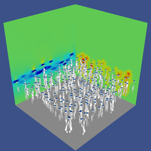
At a qualitative level, figure 5(a) shows the instantaneous motion of the bubbles at an early stage of the rising. The vorticity generated by the bubbles is included in elongated wakes. At this time, the transient has approximately finished and the thin layer of bubbles has stabilised to a width of approximately  $7d_b$. A video is also given as supplementary material available at https://doi.org/10.1017/jfm.2021.288 to help the reader to have a clearer idea of the set-up.

Figure 5. (a) Snapshot of the 3-D simulation at  $t=6$ after the release (a). Time is made non-dimensional with the bubble buoyancy time $\sqrt {d_b/g}$. The VOF field is shown with blue isosurfaces and the $\lambda _2$ vorticity field is shown with grey contours. The right-hand wall displays the level of mesh adaptation, while the left-hand wall displays the vertical component of the velocity field. (b) Bubble positions at different times, $t=6$ and $t=9$. Positions on the $y$ direction are collapsed on the plane. The lines correspond to the interrogation window.
In the same figure 5(b) we can see a lateral 2-D projection of the domain showing bubble positions at  $t=6$ and at $t=9$, that is the last time used for the statistical analysis. The same procedure as in 2-D has been followed to acquire data and compute observables, with an interrogation window composed by the horizontal planes between $z=22$ and $z=25$, see figure 5(b).
We have acquired the data from each cell in this domain, i.e. considering both phases, and used them to compute the statistics in the time range  $t\in [8.6,9.2]$. That approximately corresponds to the range over which bubbles are present in the whole window. More specifically, at $t=9.4$ only few bubbles are still present, and the statistics computed at $t=9.6$ turn out to be already strongly damped, as in earlier studies fluctuations are rapidly (exponentially) attenuated behind the swarm (Risso Reference Risso2018). In this time range, statistics are found to be roughly homogeneous in the interrogation window. We have, therefore, averaged over this space window to get better statistics, as done in the 2-D case. Statistics have been found to be also approximately steady in the time range considered, but with significant fluctuations and we have preferred to avoid time averaging. Such a choice for the statistical analysis region excludes the initial transient regime that concerns only the first few times. We display in figure 6 the p.d.f. of the vertical $z$ and horizontal $x$ velocity fluctuations (the $y$ component does not present appreciable statistical differences with respect to the $x$ component). As in the 2-D case, the velocity fluctuation field is computed at each $z$ subtracting the average velocity computed over the corresponding plane ${\boldsymbol u^\prime }={\boldsymbol U}-\langle \boldsymbol U \rangle _z$. We find the same characteristics reported in experiments (Riboux et al. Reference Riboux, Risso and Legendre2010), against which results are compared. The vertical velocity is strongly skewed, indicating a more important probability of having positive fluctuations, while the horizontal components are symmetric. Furthermore, both components are non-Gaussian, which is related to the complex features of the bubble-induced agitation. The agreement between numerical simulations and experiments is globally good. Yet in the numerical experiment the extreme events tend to be more frequent than in experiments, and exponential tails are found for $\sigma >rsim 3$. This may be related to the fact that the flow is here unsteady, and experiments may be under-sampling extreme events because they plausibly filter the smallest scales, and to the different measurement protocol. Since the p.d.f. of both components have been measured only in the experiments by Riboux et al. (Reference Riboux, Risso and Legendre2010), it is difficult to conclude. Finally, with respect to the 2-D case, figure 4, the p.d.f. is more skewed in the 3-D case. That is consistent with what is observed in experiments in a swarm confined in a thin gap (Bouche et al. Reference Bouche, Roig, Risso and Billet2014), although the wall friction effect is important there and thus the comparison is not conclusive. In figure 7(a), we present the spectrum of the kinetic energy computed in the same window. To compute the spectra, we have interpolated the data on a regular grid. To avoid spurious errors, we have eliminated the highest wave modes, so that spectra are calculated for 512 modes, although the maximum refinement is up to 4096 points. As for 2-D simulations, we have computed the spectrum at different times (not shown here), and we have found very little difference if spectra are computed at those times when bubbles are present in the plane used for the computation. When the bubbles have left the spatial region under investigation for a few characteristic times, agitation then decays rapidly, and an exponential fall-off is recorded. Figure 7(a) shows that bubbles are able to generate significant fluctuations in the length range $\lambda \in [10d_b,0.1 d_b]$, before being dissipated. After the energy range $\lambda \in [10d_b,1 d_b]$, the spectrum follows a power law with a scaling $E(k) \sim k^{-3}$ in an inertial range over the decade $\lambda \in [d_b,0.1 d_b]$. No hint of an inertial range with slope $k^{-5/3}$ is observed, neither at large or small scales.

Figure 6. Probability density functions of the velocity fluctuations in the lateral  $x$ direction (a), and in the vertical $z$ (b), at time $t=9$, averaged over the space window $z=22\text {--}25$. Results are compared with the experimental data by Riboux et al. (Reference Riboux, Risso and Legendre2010), for a concentration of $\phi =1.7\,\%$, close to that of the numerical configuration. The points have been extracted directly from Risso (Reference Risso2018), and show the results obtained from measurement of the liquid agitation within the swarm. The error bars indicate the fluctuations recorded in the time range $t\in [8.6\text {--}9.2]$.

Figure 7. (a) Normalised spectrum of the kinetic energy. Present results ( $Ar = 185$ and $Eo= 0.28$) are displayed at $t=8.8$ averaged over the space window $z=22\text {--}25$. The dashed line represents the $-3$ slope. Data obtained by Pandey et al. (Reference Pandey, Ramadugu and Perlekar2020) are shown for comparison at two different $Ar$ numbers. (b) Vorticity field for bubbles at $t=9.0$ and $z=25d_b$.
For comparison, the very recent numerical results presented by Pandey et al. (Reference Pandey, Ramadugu and Perlekar2020) are also shown for two  $Ar$ numbers. It is worth recalling that these results have been obtained with a lower resolution ( $24$ points per diameter instead of $82$ for the present simulation), and using a much lower density ratio of approximately $20$, instead of $800$ for the present simulation as for water/air. Despite these important differences, the results obtained in the present DNS are in quite good agreement with those obtained in Pandey et al. (Reference Pandey, Ramadugu and Perlekar2020) at $Ar=358$. A departure from DNS only appears at small scales around $1/10 d_b$, plausibly because of the lower resolution (256 points used in LES against 4096 used in the DNS here). The other simulation at $Ar=113$ seems instead to decay faster at all scales. We compare the results also against experiments. It can be observed that numerical and actual experiments do not investigate the same scales. Experiments are able to access a much larger domain, and they suggest that the $k^{-3}$ scaling might be valid over a larger range than that displayed in our results. On the other hand, numerical simulations appear to be more adequate to analyse accurately the small scales, where a possible change of slope from the Kolmogorov one is not recorded. Moreover, it is important to note that in experiments spectra are computed just behind the swarm, and not within it as in simulations. This may have an effect at small scales.
In order to qualitatively complement this analysis, we show in figure 7(b) the vorticity field on the same plane used to compute the spectra. This field highlights the position of the bubbles and the generation of vorticity at the scale of the diameter and slightly more. Several bubbles are still present at this time. In some cases it is apparent that different vortices have interacted, producing more complex structures.
While energy spectra contain key information about the flow, they cannot be used to disentangle the different mechanisms leading to the observed scalings, and a scale-by-scale analysis can be particularly useful (Alexakis & Biferale Reference Alexakis and Biferale2018). For that purpose, we apply a coarse-graining approach (Duchon & Robert Reference Duchon and Robert2000; Eyink & Sreenivasan Reference Eyink and Sreenivasan2006b) linked to the filtering approach used in LES (Germano Reference Germano1992), and recently applied to different turbulent configurations (Chen et al. Reference Chen, Ecke, Eyink, Rivera, Wan and Xiao2006b; Xiao et al. Reference Xiao, Wan, Chen and Eyink2009; Faranda et al. Reference Faranda, Lembo, Iyer, Kuzzay, Chibbaro, Daviaud and Dubrulle2018; Dubrulle Reference Dubrulle2019; Valori et al. Reference Valori, Innocenti, Dubrulle and Chibbaro2020). More specifically, we have applied this methodology to the velocity field, obtaining information about the energy flux and the dissipation. The advantage with respect to a spectral approach is that one can gain details also on the locality of the cascade, differentiating regions with positive or negative fluxes. Moreover, this spatial filtering approach is positive definite and local in space and can, therefore, be applied also in non-homogeneous flows.
In this filtering approach, the dynamic velocity field  ${\boldsymbol u}$ is spatially (low-pass) filtered over a scale $\ell$ to obtain a filtered value $\bar {{\boldsymbol u}}_\ell ({\boldsymbol x})$ as follows:
 \begin{equation} \bar{{\boldsymbol u}}_\ell({\boldsymbol x}) = \int \textrm{d}^3 \,r G_\ell({\boldsymbol r}) {\boldsymbol u}({\boldsymbol x}+{\boldsymbol r}),\end{equation}
where  $G_\ell$ is a smooth filtering function, spatially localised and such that $G_\ell (\boldsymbol r) = \ell ^{-3}G(\boldsymbol r/\ell )$ where the function $G$ satisfies $\int \textrm {d}\boldsymbol r \, G(\boldsymbol r)=1$, and $\int \textrm {d}\boldsymbol r \, \vert \boldsymbol r \vert ^2 G(\boldsymbol r) = O(1)$. By applying the filtering to the Navier–Stokes equations for the liquid phase we obtain the coarse-grained dynamics
 \begin{equation} \partial_{t} \bar{{\boldsymbol u}}_\ell+ (\bar{{\boldsymbol u}}_\ell \cdot {\boldsymbol{\nabla}})\bar{{\boldsymbol u}}_\ell ={-}\dfrac{1}{\rho}{\boldsymbol{\nabla}}\bar{p}_{\ell} -{\boldsymbol{\nabla}}\cdot{\boldsymbol{\tau}}_\ell+\nu\nabla^{2}\bar{{\boldsymbol u}}_\ell . \end{equation}
Since we focus on the liquid agitation, we neglect the gravity contribution, which acts as power injection through bubbles. In the same vein, at interfaces surface tension and density effects play a role. However, few bubbles are present in the analysed region, so that the impact should be small and we may retain the single-phase formulation given by (6.2). Furthermore, we are mainly interested at understanding whether a cascade process is active. To address this issue, the key term is given by  ${\boldsymbol {\tau }}_\ell$, subscale stress tensor (or momentum flux), which describes the force exerted on scales larger than $\ell$ by fluctuations at scales smaller than $\ell$. It is given by
 \begin{equation} ({\boldsymbol{\tau}}_\ell)_{i,j} =\overline{(u_i u_j)}_\ell - (\bar{u}_\ell)_i (\bar{u}_\ell)_j . \end{equation}
The corresponding pointwise kinetic energy budget reads
 \begin{equation} \partial_t \left(\tfrac{1}{2}|\bar{\boldsymbol u}|^2\right) + \partial_j \widetilde{{ q}}_j={-}\varPi_\ell - \nu|{\boldsymbol{\nabla}}\bar{\boldsymbol u}|^2,\end{equation}
where we have dropped the  $\ell$ subscript whenever unambiguous for the sake of clarity, and
 \begin{equation} \widetilde{{ q}}_j=\left[ \left(\frac{1}{2}|\bar{\boldsymbol u}|^2 + \dfrac{1}{\rho}\bar{p} \right)) \bar{u}_j + \tau_{ij}\bar{u}_i - \nu\partial_j\left(\frac{1}{2}|\bar{\boldsymbol u}|^{2}\right)\right];\quad \varPi_\ell({\boldsymbol x}) \equiv{-}(\partial_{j}\bar{u}_{i})\tau_{ij}, \end{equation}
where  $\widetilde {{\boldsymbol q}}_\ell$ is the transport term and $\varPi _\ell$ is the sub-grid scale (SGS) energy flux. This term is key since it represents the space-local transfer of energy among large and small scales across the scale $\ell$. The term $\varPi _\ell$ identifies the presence of a local direct (positive) or inverse (negative) energy cascade according to its sign. The last term in (6.4) represents the coarse-grained dissipation $\epsilon _\ell =\nu |{\boldsymbol {\nabla }}\bar {\boldsymbol u}|^2$. If a spatial average is done for different values of the filter width, one can find the average transfer of energy at each scale. Since our configuration is non-homogeneous in the vertical direction, the transport term $q_j$ in (6.4) is not zero. Yet, this term is related to spatial redistribution of energy and not directly linked to the cascade process, contrarily to $\varPi _\ell$ and $\epsilon _\ell$. For this reason, we have not analysed those terms.
In this work, we have applied a Gaussian filter defined as
 \begin{equation} G ({\boldsymbol r}) = \sqrt{\frac{6}{\rm \pi}} \exp({-}6 {\boldsymbol r}^2), \end{equation}
as typically used in LES (Pope Reference Pope2000). Since the flow is homogeneous in the horizontal direction, the filtering can be efficiently performed in spectral Fourier space, multiplying the quantity to be filtered by the Fourier transform of the filter
 \begin{equation} \hat{G}_\ell ({\boldsymbol k}) = \exp({-}k^2 \ell^2/24), \end{equation}
and then transforming back into physical space. In figure 8(a), we show the fluxes computed from the coarse-grained quantities defined in (6.5a,b). It is worth emphasising that fluxes are averaged in space but not in time. The physical features which unfold are the following.
(i) The scale-by-scale fluxes show variability in time, pointing out the statistical unsteadiness of the transfer processes.
(ii) Both inverse (negative flux) and direct (positive flux) cascades are found at different times. Both cascades involve more than a decade of scales. The direct cascade is more significant at scales smaller than the diameter, and the inverse cascade at scales larger than it.
(iii) Energy is transferred from scales around $\ell \approx d_b/2$ in both directions.
(iv) At around the same length scale the dissipation becomes significant.
(v) At smaller scales dissipation and direct flux become comparable.


Figure 8. (a) Mean energy flux at different filter lengths, the energy flux (solid lines) and the dissipative flux (dashed lines) are displayed at different times. Fluxes are computed at  $z=25d_b$, the same as for the computations of spectra. The length scale displayed on the $x$ axis is normalised with the diameter $d_b$, so that $\ell =1$ corresponds to the initial bubble diameter. (b) Local energy flux at $t=9$ and $z=25d_b$. In the upper half-panel the filter length is $l=0.5 d_b$, in the lower half-panel $l=0.1 d_b$. The colour scale is the same in both half-panels. Each slice is made by $450$ points taken in the horizontal direction, and $180$ in the vertical direction.
Our scale-by-scale analysis points to the following physical picture of the pseudo-turbulent agitation induced by bubbles. Energy is injected by buoyancy (the only force at play here) and transferred by the bubbles into the liquid via the interface at scales comparable to the bubble diameter. The energy input  $W_b$ must be proportional to the work made by buoyancy: $W_b \sim \phi g U_b$. Dissipation becomes significant at $\ell \sim d_b$, showing that fluctuations are mostly dissipated inside the small structures generated by bubble wake-interactions. At smaller scales than the diameter, there is a range where $W_{diss} \approx W_b$, which means $\nu (\delta u_\ell )^2\ell ^2 \sim \phi g U_b$, where we have considered the two-point quantities $\delta u_\ell =u(x+\ell )-u(x)$. This gives the scaling behaviour $\delta u_\ell ^2 \sim \ell ^2$, which means in spectral space $E(k) \sim k^{-3}$. We obtain here the scaling with an argument similar to that used by Lance & Bataille (Reference Lance and Bataille1991) and Prakash et al. (Reference Prakash, Mercado, van Wijngaarden, Mancilla, Tagawa, Lohse and Sun2016), yet in the physical space rather than in the spectral one. The fact that $\varPi _\ell$ changes sign shows that both a direct and an inverse transfer of energy through nonlinear terms are active, and dominate at different times. On average the transfer is more towards small scales, but the inverse process is not negligible. The copresence of direct and inverse cascades intermittently is a feature also of fluid turbulence (Chorin Reference Chorin2013). While the direct transfer is linked to dissipation, the inverse one is related to the formation of the wakes, which are found to develop up to some characteristic lengths.
To further understand the mechanisms indicated, we show in figure 8(b) a slice of the energy flux at two different scales: half the diameter and a smaller scale. The pictures show that the energy flux and dissipation are concentrated in the wakes generated by the bubbles. Furthermore, these structures, initially at the scale of the diameter, may become a little larger, indicating the generation of larger eddies, and are eventually dissipated at small scales, where the imprint of the bubbles is still detectable.
7. Conclusions
We have numerically investigated buoyancy-driven bubbly flows, focusing on the agitation induced by the bubbles on the fluid. The purpose of the study was to characterise the physics of the collective motion induced when many bubbles rise under the sole effect of gravity. We have carried out several 2-D and 3-D preliminary tests and the first high-resolution DNS of a 3-D realistic bubble column.
We have first extensively investigated the interplay between the numerics and the physics of bubbly flows at moderate and high Reynolds numbers in order to properly set numerical parameters compatible with a reliable description of the flow. To do so, we studied different configurations and compared the results with recent studies made using different interface advection methods. These numerical experiments have shown on the one hand that the physical parameters, and most notably the density ratio of the two fluids, may affect the results both qualitatively and quantitatively. On the other hand, to be sure to have solution at convergence, the spatial resolution should be increased when increasing the  $Re$ number. In particular, to carry out a DNS it seems necessary to fulfil the following criteria: (i) the density ratio has to be realistically high $\rho _l/\rho _b > 100$; (ii) the viscosity ratio should also be realistic $\mu _l/\mu _b \approx 100$; (iii) the number of points used to resolve the bubbles must increase linearly with the Archimedes number (or the Reynolds number based on the raising velocity). As a rule of thumb, this number should be of the order $d_b/\varDelta \approx {Ar}/2$.
Given the numerical constraints which do not allow a parametric DNS study of a high Reynolds flow in three dimensions, we have rather performed a comprehensive analysis of the agitation in a 2-D bubble column at moderate and high Reynolds numbers with a volume fraction of approximately  $5\,\%$ in the bubble layer, in order to prepare a 3-D study. Both unsteady and steady numerical experiments have been carried out. In this configuration, we have analysed the velocity fluctuations and find different behaviour for different Reynolds numbers, even if the $-3$ slope of the spectra seems to be a robust feature of this type of flow, also in two dimensions. That highlights that the same spectrum is consistent with different mechanisms. At higher Archimedes number, the nonlinear interactions start to play an important role, and in particular the presence of an inverse cascade at scales larger than the diameter has been found for flows at $Ar$ number higher than $100$. Indeed, at larger scales than the diameter, where the dissipation is negligible, the energy budgets is $\varPi _\ell \sim W_b \approx \phi g U_b$ which gives the Kolmogorov scaling $\delta u_\ell ^2\sim \ell ^{2/3}$, or $E(k) \sim k^{-5/3}$, typical of an inverse cascade. As expected, p.d.f.s show a strong anisotropy of the fluctuations in the vertical direction, while horizontal fluctuations are symmetric. The 2-D simulations have indicated that the statistics obtained in unsteady simulations are accurate, provided the space window used to analyse the data is well chosen. We have provided all the criteria to be fulfilled to get a reliable numerical experiment. Besides the main numerical relevance, the configuration may have some similarity to that investigated experimentally in a confined 2-D configuration (Bouche et al. Reference Bouche, Roig, Risso and Billet2012, Reference Bouche, Roig, Risso and Billet2014).
Then, on the basis of the results obtained in the first part of our work, we have performed a single numerical experiment of a 3-D bubble column at  $Ar =185$, which corresponds to a Reynolds number consistent with experiments ( $Re\approx 500$). First we have observed that the one-point p.d.f. of the velocity fluctuations in numerical simulations are in agreement with those obtained experimentally (Riboux et al. Reference Riboux, Risso and Legendre2010; Risso Reference Risso2018). However, the tails related to rare events ( ${>}3 \sigma$ from the mean) are more pronounced, with an exponential decay, than in the experiments where they are more Gaussian. It is difficult to say if this discrepancy is due to the strong unsteadiness of the flow, or to a smoothing of extreme events in real experiments because of the different measurement procedure.
The energy spectra have also been analysed and compared with recent numerical simulations performed at low resolution and low density ratio. We have found a  $k^{-3}$ scaling over a decade of scales smaller than the diameter, and possibly at scales just a little larger. We have not found any hint of a Kolmogorov $k^{-5/3}$ scaling, neither at large nor small scales. Comparison with experimental spectra do not add much insight, and indicates that experiments are more useful to analyse large scales, whereas simulations are better fitted for the small ones.
We have shown through a scale-by-scale analysis in physical space that the spectra are related to a nonlinear cascade mechanism, and do not reflect only the presence of wakes. Indeed we have found that a flux of turbulent kinetic energy is present in the range of scales going from  $2d_b$ up to $d_b/20$, where dissipation becomes dominant. In this range the balance between the flux of energy and the dissipation explain the $k^{-3}$ scaling. Interestingly our unsteady numerical experiment highlights the presence of instantaneous fluxes in both directions indicating the tendency to create locally larger structures around the bubbles, even though on average the energy is injected around the bubble diameter scale and mostly transferred to smaller scales where it is eventually dissipated. Considering both 2-D and 3-D results, it can be inferred that in all cases an agitation is produced by the geometrical structure, as modelled by Risso (Reference Risso2011), while a nonlinear cascade process is superimposed at high $Ar$. An important result of our work comes also from the comparison with the recent simulations by Pandey et al. (Reference Pandey, Ramadugu and Perlekar2020). According to our analysis these simulations should be considered as implicit LES when $Ar>50$, given the low resolution with respect to the bubble size, yet they are representative of the numerical resolution used in most of the works presently carried out in turbulent bubbly flows (Elghobashi Reference Elghobashi2019; Cifani, Kuerten & Geurts Reference Cifani, Kuerten and Geurts2020). The present DNS results show that one-point and two-point statistics are in good agreement with the results of Pandey et al. (Reference Pandey, Ramadugu and Perlekar2020) obtained at high $Ar$ number, except at small scales. The present conclusion is hence that using only 20–30 points to resolve the bubble diameter, seems to be sufficient to get consistent results with respect to large-scale statistics, although finite Reynolds number effects are found to be exaggerated. At variance with what was found for single-bubble observables (Cano-Lozano et al. Reference Cano-Lozano, Martinez-Bazan, Magnaudet and Tchoufag2016a), our fully resolved DNS validate the use of under-resolved simulations to analyse large-scale collective properties in bubble-induced agitation.
Concerning future developments. In this work we have focused on liquid agitation properties, but bubble properties deserve to be studied as well, as done in experiments (Bouche et al. Reference Bouche, Roig, Risso and Billet2012; Risso Reference Risso2018). We have been performing the Lagrangian tracking of the bubbles, and notably it would be relevant to get insights on the bubble distribution within the flow. We hope to have further results in the future. With respect to simplified physical modelling (Risso Reference Risso2016, Reference Risso2018), we plan to carry out steady simulations at different  $Re$ numbers to analyse some assumptions that could not be assessed in the present framework. It would be also interesting to analyse the budgets of the momentum and energy equation in relation to the development of two-fluid models, that is Reynolds-averaged Navier–Stokes (RANS) (Drew Reference Drew1983; Biesheuvel & Wijngaarden Reference Biesheuvel and Wijngaarden1984; Drew & Passman Reference Drew and Passman2006). Indeed, this is an important ongoing research for applications, and issues concerning both the stability and the quality of the models remain to be addressed (Prosperetti & Jones Reference Prosperetti and Jones1987; Davidson Reference Davidson1990; Tiselj & Petelin Reference Tiselj and Petelin1997; Song & Ishii Reference Song and Ishii2001; Panicker, Passalacqua & Fox Reference Panicker, Passalacqua and Fox2018; Du Cluzeau et al. Reference Du Cluzeau, Bois and Toutant2019; Moore & Balachandar Reference Moore and Balachandar2019; du Cluzeau, Bois & Toutant Reference du Cluzeau, Bois and Toutant2020; Du Cluzeau et al. Reference Du Cluzeau, Bois, Toutant and Martinez2020). Finally, it would be interesting to make a comparison with the somewhat similar yet different problem of the dynamics of solid finite-size particles. So far, the research has focused on suspensions of small particles (Guazzelli & Morris Reference Guazzelli and Morris2011) or large particles in media of similar density (Kidanemariam & Uhlmann Reference Kidanemariam and Uhlmann2014; Picano, Breugem & Brandt Reference Picano, Breugem and Brandt2015). Different boundary conditions on the interface should make a difference. Bubble deformability constitutes another key element (Clift et al. Reference Clift, Grace and Weber2005) but, for instance in the regime investigated in the present work, the impact should be small.
Supplementary movie
Supplementary movie is available at https://doi.org/10.1017/jfm.2021.288.
Acknowledgements
This work was granted access to the HPC resources of [TGCC/CINES/IDRIS] under the allocation 2019- [A0062B10759 and A0082B10759] attributed by GENCI (Grand Equipement National de Calcul Intensif). We thank R. Fox for fruitful discussions.
Declaration of interests
The authors report no conflict of interest.
Appendix A. Arrays of bubbles
For the test case proposed by Esmaeeli & Tryggvason (Reference Esmaeeli and Tryggvason1999), displayed in figure 1(a), the details of the different grids are reported in table 3, together with the steady values of the Reynolds number.
Table 3. Grid resolutions and final Reynolds number for the 3-D array of bubbles.

The parameters of the simulations of the case of the oblique array of bubbles are reported in table 4. The results not shown in the main text are given in figure 9, and summarised in table 5. Similar regimes are captured in each case, while the transition may occur at different times compared with Loisy et al. (Reference Loisy, Naso and Spelt2017), since it is triggered by numerical asymmetry. For the same reason, while we expect a quantitative agreement in the direction of gravity, the other two components can share the energy in a different way, provided that this is compatible with the symmetry of the problem. As shown in table 5, the steady value of the different components of the bubble Reynolds number is in excellent agreement for regimes a and b, while in regime c where a steady state is not reached the agreement is more qualitative. The oscillation periods appear also to be in qualitative agreement.

Figure 9. Time evolution of two components of the bubble Reynolds number for regime b (panel (a)) and regime c (panel (b)).
Table 4. Non-dimensional parameters for the 3-D-oblique array of bubbles test case.

Table 5. Final  $Re$ for the 3-D-oblique test case. For the last oscillating regime we have reported the average over the last steps, so the comparison is to be considered qualitative.

Appendix B. Technical issues
B.1. Grid refinement effects
We have replicated some of the results obtained by Cano-Lozano et al. (Reference Cano-Lozano, Martinez-Bazan, Magnaudet and Tchoufag2016a) to study the behaviour of a single bubble rising ‘in a large tank’, i.e. far from any boundaries. The physical parameters chosen are the same used in the 3-D bubble column. Namely, we fix  $Ar =185$ and $Eo= 0.28$. The acceleration of gravity is set to unity, which gives a characteristic rise velocity also of order unity, and a maximum time for the simulation comparable to the domain size. In this regime, it turns out that bubble trajectories are between the rectilinear and chaotic regimes, as found in the original paper (Cano-Lozano et al. Reference Cano-Lozano, Martinez-Bazan, Magnaudet and Tchoufag2016a). We have simulated the bubble rise with three different grids, namely varying the threshold of the error tolerance, fixed at $err_v=0.001; 0.003; 0.01$, in absolute value. This threshold controls the local refinement of the grid (van Hooft et al. Reference van Hooft, Popinet, van Heerwaarden, van der Linden, de Roode and van de Wiel2018). In figure 10(a), we show the evolution of the rise velocity of the bubble, which is given by the Reynolds number in dimensionless form. The two low-tolerance grids show very little difference (less than $1\,\%$), whereas for the highest-tolerance grid the difference is of the order of $5\,\%$. This indicates that the three grids are sufficient to get a qualitative reproduction of the physics of the problem but that only the two more refined are at convergence. In figure 10(b), we display the evolution of the number of grid points with time for the three different grids. This gives a measure of the computational cost of each set-up. From figure 10(a), we can see that a transient is present with a duration of approximately $8\div 10$ unit times. Results show that an over-refinement of the bubble is present for the lowest error threshold. We have, therefore, found that convergence is reached with $N_{Max}=2^{12}$, such that the maximum refinement is of $82$ points per diameter, with an error threshold of $0.003$ (absolute value) in the velocity. This resolution has hence been chosen for the final 3-D bubble column simulation.

Figure 10. (a) Average Reynolds number of a single bubble rise plotted for the three resolutions. The final values are  $Re=559$ for $e_v=0.01$, $Re=549$ for $e_v=0.003$ and $Re=547$ for $e_v=0.001$. (b) The number of mesh points is plotted against time. It should be noted that the number of points is approximately steady for the two coarser resolutions, while it is growing rapidly for the most refined resolution.
B.2. Coalescence
We have studied from a qualitative point of view the coalescence of two bubbles in relation to density ratio and grid refinement. This is a vast area of research (Liao & Lucas Reference Liao and Lucas2010) and a detailed analysis of this issue is beyond the scope of the present work. Yet, in the concentration regime studied in the present work ( $\phi <5\,\%$) coalescence and breakup have a negligible effect (Jha & Govardhan Reference Jha and Govardhan2015) and it is, therefore, important to have some control on this process to avoid spurious effects. In particular, it is known that VOF methods tend to make coalescence too easy (Scardovelli & Zaleski Reference Scardovelli and Zaleski1999), if numerical parameters are not well chosen. Here we consider for this purpose two bubbles in a 2-D box of side $20$ times the diameter of the bubbles with periodic boundary conditions. The physical parameters are fixed in such a way that dimensionless numbers are $Ar =30$, $Eo=0.1$ and $\mu _b/\mu _l=100$. We consider two bubbles, one on top of the other, initially at rest in a quiescent fluid. The top bubble is at $0.75$ diameter from the bottom bubble. The situation is somewhat similar to that encountered by bubbles at the initial stage of our bubble-column simulations. They start moving because of buoyancy which induces vorticity fluctuations and creates wakes. We shall consider our numerical approach acceptable if coalescence is avoided. We have first fixed the density ratio $\rho _l/\rho _b=1000$, and varied the resolution with different grids. We have found that convergence is attained with $N_{Max}=2^{12}$, since the results are the same as those obtained with $N_{Max}=2^{13}$. Using $N_{Max}=2^{11}$ instead the coalescence occurs (results not shown here). Two instants for the maximal resolution are displayed in the bottom of the figure 11. Then, we have assessed the influence of the density ratio. We have chosen the finest resolution $N_{Max}=2^{13}$ to be sure to avoid any discretisation effect. In figure 11, we show two instants of this dynamics, displaying also the vorticity field, for two different density ratios. Notably, in panels (a,c) we display the results obtained for a density ratio of $\rho _l/\rho _b=100$, for which coalescence happens. In panels (b,d) we show the same case but with a density ratio of $\rho _l/\rho _b=1000$. As said previously, in this case coalescence does not occur. We have investigated different density ratios in the range $\rho _l/\rho _b\in [10,1000]$ (not shown here for the sake of clarity), and it turns out that in our particular set-up the threshold for avoiding the coalescence is approximately $\rho _l/\rho _b=200$.

Figure 11. Contour plot of the vorticity at two instants. The grid is drawn to show the degree of refinement obtained with  $N_{Max}=2^{13}$, other resolutions are not shown for the sake of simplicity. (a,c) simulation with $\rho _l/\rho _b=100$; (b,d) simulation with $\rho _l/\rho _b=1000$.
Appendix C. Two-dimensional pseudo-turbulence: complements
In figure 12, we show the spectra of both the vertical and horizontal velocity fluctuations made non-dimensional with  $\sqrt {d_b/g}$. They are displayed at different times, and in the space windows $z\in [15\text {--}20],[20\text {--}25]$. Only the case at $Ar =100$ is shown for the sake of clarity, since the results for the other $Ar$ numbers are similar. Horizontal and vertical spectra are similar. Moreover, the same information content is present in both spatial windows, for all the spectra computed within the swarm are equivalent, that is at $t\in [10\text {--}16]$ for $z\in [15\text {--}20]$, and in the whole time-window for $z\in [20\text {--}25]$. Instead, a few characteristic times after all bubbles have gone out from the interrogation window, the spectrum starts to decay exponentially, as indicated by the spectra computed at $t=20$ in the space window $z\in [15\text {--}20]$. We have observed in figure 2 a possible $k^{-5/3}$ range at large scales in the spectra of the 2-D case at high $Ar$. The scaling range is, however, tiny and, therefore, to corroborate the claim of an inverse cascade we show in figure 13, the scale-by-scale energy flux, as defined in the discussion of the 3-D results, see (6.5a,b). The flux turns out to be negative at scales larger than approximately half of the diameter. That is in line with the spectra, confirming the presence of an inverse cascade, as already found in recent simulations of a 2-D mixture at very low density ratio (Ramadugu, Pandey & Perlekar Reference Ramadugu, Pandey and Perlekar2020).

Figure 12. Spectra of the vertical (a,c) and horizontal component (b,d) of the velocity for bubbles with  $Ar = 100$ and $Eo= 0.1$ evaluated at different times. Panels (a,b) correspond to the spatial window between $15$ and $20$ diameters, panels (c,d) to the one between $20$ and $25$ diameters. The energy spectrum is made non-dimensional with the corresponding standard deviation.

Figure 13. Mean energy flux, (6.5a,b), with different filter lengths. The time average is taken in the range  $t=13\text {--}23$ as in panel (a).


 Open access