


1. INTRODUCTION
The Global Positioning System (GPS) and Inertial Navigation System (INS) have complementary operational characteristics and the synergy of both systems has been widely explored (Brown and Hwang, Reference Brown and Hwang1997; Farrell and Barth, Reference Farrell and Barth1999). The GPS/INS integrated navigation system is the adequate solution to provide a navigation system that has superior performance in comparison with either GPS or INS stand-alone system. Traditional GPS/INS integration designs use a loosely or a tightly coupled architecture. The loosely coupled integration uses the GPS derived position and velocity as the measurements. This architecture is sub-optimal from the standpoint of preventing GPS outages (i.e., with less than four available satellites). A tightly coupled GPS/INS navigation filter blends the GPS pseudorange and inertial measurements and obtains the vehicle navigation solution. The ultra-tightly coupled architecture combines the I (in-phase) and Q (quadrature) correlator components in the receiver signal tracking loops and the INS navigation filter function into a single integrated filter (Babu and Wang, Reference Babu and Wang2004, Reference Babu and Wang2005, Reference Babu and Wang2009; Yuan and Zhang, Reference Yuan and Zhang2009).
In the ultra-tightly coupled integration mode, the correlator variables I and Q are given as measurements to the integration filter. Estimated Doppler offsets can be used to maintain tracking in the tracking loop, either under high dynamics or GPS signal outages (Alban et al., Reference Alban, Akos and Rock2003, Reference Alban, Akos, Rock and Gebre-Egziabher2004; Babu and Wang, Reference Babu and Wang2004, Reference Babu and Wang2005). The inherent property of this system is the integration of INS derived Doppler feedback to the carrier tracking loops. This architecture shows an important advantage of this system: as the INS Doppler aiding removes the vehicle Doppler from the GPS signal, it facilitates a significant reduction in the carrier tracking loop bandwidth; on a comparative scale the dynamics on the PseudoRandom Noise (PRN) code is very much less due to its low frequency nature. The bandwidth reduction improves the anti-jamming performance of the receiver, and also increases the post correlated signal strength. In addition, due to lower bandwidths, the accuracy of the raw measurements is also increased.
The Kalman Filter (KF) (Brown and Hwang, Reference Brown and Hwang1997; Gelb, Reference Gelb1974) is a well known sequential data assimilation scheme for solving the Wiener problem. In the current integration scenarios, the navigation filter is commonly designed by use of a KF or its nonlinear version, Extended Kalman Filter (EKF) to estimate the vehicle state variables and suppress the navigation measurement noise. Other alternatives were proposed for GPS/INS integration. The popular alternatives include the Unscented Kalman Filter (UKF) (Julier, Reference Julier2002; Julier et al. Reference Julier, Uhlmann and Durrant-whyte1995, Reference Julier, Uhlmann and Durrant-Whyte2000; Julier and Uhlmann, Reference Julier and Uhlmann2002; Wan and van der Merwe, Reference Wan and van der Merwe2000, Reference Wan, van der Merwe and Simon2001) and the Particle Filter (PF) (Djuric et al., Reference Djuric, Kotecha, Zhang, Huang, Ghirmai, Bugallo and Miguez2003; Rubin, Reference Rubin, Bernardo, DeGroot, Lindley and Smith1988; Aggarwal et al., Reference Aggarwal, Syed and El-Sheimy2009; Doucet et al., Reference Doucet, de Freitas, Gordon, Doucet, de Freitas and Gordon2000; Gordon et al., Reference Gordon, Ristic and Arulampalam2004). In the ultra-tightly coupled GPS/INS modes, the EKF (Babu and Wang, Reference Babu and Wang2009) and UKF (Yuan and Zhang, Reference Yuan and Zhang2009) have been employed to implement the ultra-tight navigation filter.
Proposed by Julier, et al. (Reference Julier, Uhlmann and Durrant-whyte1995) to address nonlinear state estimation in the context of control theory, the UKF is a nonlinear, distribution approximation method that uses a finite number of carefully chosen sigma points to propagate the probability of state distribution. The UKF approximates the Gaussian distribution by a set of deterministically selected samples called the sigma points, which are propagated through the true non-linear models to capture the true mean and covariance of transformed distribution. The UKF made a Gaussian approximation with a limited number of sigma points through the Unscented Transform (UT) (Julier, Reference Julier2002; Julier and Uhlmann, Reference Julier and Uhlmann2002; Julier et al., Reference Julier, Uhlmann and Durrant-Whyte2000). Through the nonlinear dynamics of the system, the true mean and covariance of the Gaussian Random Variable (GRV) are completely captured with a minimal set of samples. The basic premise behind the UKF is that it is easier to approximate a Gaussian distribution than it is to approximate an arbitrary nonlinear function. The posterior mean and covariance can be captured accurately to the second order of Taylor series expansion for any nonlinear system.
For certain problems, a Gaussian assumption cannot be applied with confidence. To overcome these problems, the probability-based estimator PF was proposed to approximate the posterior distribution for highly nonlinear systems. The Bayesian estimation is the foundation for particle filters. As a non-parametric filter, the PF can easily deal with nonlinear and/or non-Gaussian noises. A large number of particles are required to obtain reasonable accuracy as the latest measurement is totally ignored. Henceforth, many variants of these filters are suggested by a number of researchers. One such method to incorporate the most current measurement into the state vector estimation is through the local linearization, where the EKF or UKF can be used to generate the true mean and covariance of the proposal distribution. For the Unscented Particle Filter (UPF) (van der Merwe et al., Reference van der Merwe, Doucet, de Freitas and Wan2000), the UKF is incorporated to generate the proposal distribution for acquiring a maximum a posteriori probability estimate of the nonlinear system, and the importance density function can approximate the true posterior density distribution. The use of the importance proposal distribution integrates the latest observation into system state transition density, so as to properly match the a posteriori density.
The uncertainty of the process noise and measurement noise degrades the performance when implementing the filter. In various circumstances where there are uncertainties in the system model and noise description, and the assumptions on the statistics of disturbances are violated due to the fact that in a number of practical situations, the availability of a precisely known model is unrealistic. One way to take them into account is to consider a nominal model affected by uncertainty. The process model of the filter is dependent on the dynamical characteristics of the vehicle. Poorly designed mathematical models may lead to the divergence. The statistical properties of error in the system cannot be treated as unchanged, which thus results in filtering performance degradation or even divergence. An adaptive mechanism which dynamically identifies uncertainties or modelling errors can be adopted. The Adaptive Kalman Filter (AKF) approach (Ding et al., Reference Ding, Wang and Rizos2007; Hide et al., Reference Hide, Moore and Smith2003; Mehra, Reference Mehra1970, Reference Mehra1972; Mohamed and Schwarz, Reference Mohamed and Schwarz1999) has been one of the promising strategies and has been widely explored for dynamically adjusting the parameters and overcoming the divergence problem. Many efforts have been made to improve the estimation of the covariance matrices based on the innovation-based estimation approach, resulting in the Innovation Adaptive Estimation (IAE).
Fuzzy logic was first developed by Zadeh in the mid-1960s for representing uncertain and imprecise knowledge. It provides an approximate but effective means of describing the behaviour of systems that are too complex, ill-defined, or not easily analysed mathematically. One of the approaches is to employ the Fuzzy Logic Adaptive System (FLAS) (Jwo and Wang, Reference Jwo and Wang2007; Sasiadek et al., Reference Sasiadek, Wang and Zeremba2000) to adapt the gain and therefore prevent the filter from divergence. A FLAS mechanism can be incorporated for determining the factor, resulting in the Fuzzy Unscented Particle Filter (FUPF). The characteristics of the fuzzy adaptive system depend on the fuzzy rules and the effectiveness of the rules directly influences its performance. The FLAS is employed to make the necessary trade-off between accuracy and computational burden due to the increased number of particles. When the FLAS is employed, the reduced number of particles becomes accessible without significantly compromising accuracy. Two examples are provided for performance evaluation among the various data fusion methods: EKF, UKF and FLAS assisted UPF (FUPF).
The remainder of this paper is organized as follows. In Section 2, the ultra-tightly coupled GPS/INS integration is introduced. The navigation integration filter algorithm is proposed in Section 3. In Section 4, numerical experiments based on two scenarios on navigation processing are conducted to evaluate the performance for various approaches. Conclusions are given in Section 5.
2. THE ULTRA-TIGHT GPS/INS INTEGRATION
The ultra-tightly coupled GPS/INS integration architecture is shown in Figure 1. The signals from the receiver correlator, I and Q components, form the measurements of the filters. These I and Q measurements from channels {1,2, … N} are integrated with the position, velocity and attitude of the INS in a complementary filter. The code phase and Doppler shift calculated from the INS and satellite ephemeris are used to control both the code Numerically Controlled Oscillator (NCO) and carrier NCO. The number of measurement is twice of the number of satellites being used for navigation.
The received satellite signal can be presented as:
where:
A is the signal amplitude.
CA(t) is the C/A code sequence.
D(t) is the navigation data.
τ is the propagation delay between the satellite and the receiver.
f 0 is the carrier frequency.
θ 0 is the initial carrier phase.
η is the Gaussian noise.
Ignoring atmospheric and oscillator effects, the propagation delay, τ, can be expanded as
where:
P s(t s) is the satellite position at transmit time.
P r(t r) is the receiver position at receive time.
t r=t s+τ where τ is the propagation delay.
c is the velocity of light.

Figure 1. Illustration of the I and Q components as the measurements of the ultra-tightly coupled GPS/INS integration with Doppler velocity aiding.
Considering the motion of both the satellite and the receiver, the numerator of Equation (2) can be expanded using a Taylor's series into
where t 0 is the time at a reference point. Substituting (2) and (3) into (1) yields:
where:
The I and Q components of a satellite signal after correlation are represented by:

where:
 is the frequency error tracked by Frequency Lock Loop (FLL).
- is the phase error tracked by Phase Lock Loop (PLL).
k is the measurement epoch.
T is the integration interval.
η I and η Q are the noise components.
Taking expectation of the integral leads to:
which shows that E[I] and E[Q] depends on the errors of the carrier frequency and phase. These error parameters f e and θ e are described in terms of position and velocity as:
where:
P L and V L are measured position and velocity of the receiver.
- and are the receiver estimates of position and velocity.
Detailed information for the derivatives relating the I/Q and carrier phase/frequency used in the EKF can be referred to Babu and Wang (Reference Babu and Wang2009).
Doppler reflects the relative dynamics on the received radio frequency carrier. By use of the satellite ephemerides, dynamics of the GPS satellites can be known accurately, and velocity/acceleration information of the receiver can be extracted from the received Doppler signal. The Doppler calculated by the integration filter is fed into the carrier tracking loop. It is noted that when operated in the ultra-tight mode the local NCO is also updated between the navigation filter updates using the INS derived code phase and Doppler information. The following Doppler analysis is adopted from Babu and Wang (Reference Babu and Wang2004). The received Doppler frequency due to relative motion between the satellite and receiver can be modelled as:
where:
f 0 represents the carrier frequency of GPS L1 signals.
vr is the relative velocity.
e is the receiver to satellite unit vector.
c is the speed of light.
The measured Doppler frequency can be written as
where f dyn and f clk represents the Doppler due to receiver motion and receiver clock error. The INS-estimated Doppler can be modelled as:
f bias is due to systematic errors and f stoc is due to the stochastic errors of the inertial sensors. The Doppler due to receiver motion f dyn can be calculated with the aid of INS information.
where:
- is the estimated receiver's position.
- is the estimated receiver's velocity.
Subtracting Equation (14) and Equation (15) gives:
The integration filter estimates and subsequently removes the systematic error. Therefore, assuming f bias is exactly determined and removed, the effective dynamics the tracking loop needs to track becomes:
It is seen that through the Doppler frequency estimate, the tracking range can be reduced since both f clk and f stoc are small. Further information for the Doppler estimation can be referred to Babu and Wang (Reference Babu and Wang2004; Reference Babu and Wang2005), Alban, Akos and Rock (Reference Alban, Akos and Rock2003), Alban, Akos, Rock, and Gebre-Egziabher (Reference Alban, Akos, Rock and Gebre-Egziabher2004).
3. THE NAVIGATION INTEGRATION FILTER
The combination of adaptive UPF and FLAS is adopted for reducing the number of particles with sufficiently good results. The PF consists of recursive propagation of the weights and support points as each measurement is received sequentially. However, a common problem with the generic PF is the degeneracy phenomenon. To avoid the degeneracy phenomenon of the particles, one of the solving methods is to add the number of samples (or particles). However, if one adds too many particles in a filter, a large computational burden will occur. Resampling is a better method to reduce degeneracy of the algorithm. As for the resampling scheme, there are many selections such as Sampling Importance Resampling (SIR), residual resampling and systematic resampling. A good proposal distribution is essential to the efficiency of Importance Sampling (IS).
3.1. The Unscented Kalman Filter
The first step in the UKF is to sample the prior state distribution, i.e., generate the sigma points through the UT, which is a method for calculating the statistics of a random variable which undergoes a nonlinear transformation. The basic premise is that to approximate a probability distribution is easier than to approximate an arbitrary nonlinear transformation. A set of sigma points is deterministically chosen so as to capture the true mean and covariance of the random variable. The samples are propagated through true nonlinear equations and the linearization of the model is not necessary. The UKF requires less computational cost due to deterministic sampling of the sigma points as opposed to the particle filter's random particles.
The UKF is a nonlinear filter which deals with the case governed by the nonlinear stochastic difference equations:
where:
the state vector
.process noise vector
.measurement vector
.measurement noise vector
.
Both the vectors wk and vk are zero mean Gaussian white sequence having zero cross-correlation with each other:
Consider an n dimensional random variable x, having the mean ![]() and covariance P, and suppose that it propagates through an arbitrary nonlinear function f. The unscented transform creates 2n+1 sigma vectors X (a capital letter) and weighted points W, given by:
and covariance P, and suppose that it propagates through an arbitrary nonlinear function f. The unscented transform creates 2n+1 sigma vectors X (a capital letter) and weighted points W, given by:

W i(m) and W i(c) are the weights for the mean and covariance, respectively, associated with the ith point.
The sigma vectors are propagated through the nonlinear function to yield a set of transformed sigma points, yi=f(Xi), i=0, …, 2n.
The implementation algorithm of UKF is summarized as follows:
1. The transformed set is given by instantiating each point through the process model:
(21)2. Predicted mean:
(22a)3. Predicted covariance:
(22b)4. Instantiate each of the prediction points through observation model:
(23a)5. Predicted observation:
(23b)6. Innovation covariance:
(24)7. Cross covariance:
(25)8. Performing update:
(26)

3.2. The Particle Filter (PF)
Although the EKF and UKF can deal well with some nonlinear filtering problems, they always approximate p(xk|Zk) to be Gaussian, where p(xk|Zk)= pdf of xk conditioned on measurements z1, z2, …, zk.
The PF is a probability-based estimator. If the true density is non-Gaussian, PFs will provide better performances in comparison to that of EKF and UKF. Figure 2 shows the recursive Bayesian state estimation, which is based on the Bayes’ rule.
In order to compute p(xk|Zk), the equation p(xk|Zk−1) needs to be found from the Chapman-Kolmogorov equation and the marginal density function:
The pdf p(zk|Zk−1) can be obtained to be:

Figure 2. The recursive Bayesian state estimation.
The basic PFs combine two principles namely the Monte Carlo (MC) principle and the IS method where the transition prior density p(xk|xk−1) is taken as the importance distribution:
The weights of these particles are evaluated according to:
and:

where:
q(xk|xk−1, zk) is the importance density function.
w k−1 are the importance weights of the previous epoch particles.
w k are the importance weights of the current epoch.
The use of transition prior distribution as the importance distribution greatly simplifies weight calculations; however, after a few iterations, most samples have negligible weights as information coming from the latest measurement is completely ignored. In order to reduce this problem, a resampling step can be incorporated. Nevertheless, the resampling step at every time epoch can easily lead to sample impoverishment.
3.3. The Unscented Particle Filter
The importance density function is used in the Sequential Importance Sampling (SIS) and SIR schemes, where the transition prior does not take into consideration the most recent measurement data zk. Deficiency may arise in particle filters, especially when there is little overlap between the importance density function and the posterior pdf p(Xk|Zk), and the estimation result is poor. To avoid this problem that may arise from using the transition prior as the importance density function, the filter needs to incorporate the latest measurement data into it.
An improvement in the choice of proposal distribution over the simple transition prior can be accomplished by moving particles towards the regions of high likelihood, based on the most recent measurement. In a local linearization technique, utilization of the UKF within a PF framework leads to the UPF where the UKF is used to generate the true mean and covariance of the proposal distribution. This is accomplished by using a separated UKF to generate and propagate a Gaussian proposal distribution for each particle. In the UPF, each particle is drawn from the local Gaussian approximation of the optimal importance distribution p(xk|xk−1, zk) that is conditioned on the current state and the latest measurement:
where q N is representative of the Gaussian approximation of importance density and is obtained from the UKF.
An effective approach to accomplish this is to use an UKF generated Gaussian approximation optimal proposal by Julier and Uhlmann et al., (Reference Julier, Uhlmann and Durrant-whyte1995, Reference Julier and Uhlmann2002). That is:
where xki and Pki are the mean and covariance of the ith particle generated by the UKF, respectively. The ith particle at time step k is redrawn from this new updated distribution. While still making a Gaussian assumption, the approach provides a better approximation to the optimal conditional proposal distribution (van der Merwe, et al., Reference van der Merwe, Doucet, de Freitas and Wan2000).
One cycle of the UPF algorithm is summarized as follows.
3.3.1 Initialization
Assume ![]() be a set of particles sampled from the prior x0i∼p(x 0) at k=0 and set:
be a set of particles sampled from the prior x0i∼p(x 0) at k=0 and set:

where i=1…N
3.3.2. Importance Sampling
• Update each particle with the UKF to obtain mean
and covariance Pki.• Sample the particles from
, where are the estimation of mean and covariance of UKF, i=1, …, N• The recursive estimate for the importance weights can be written as follows:
(34)
where N is the number of samples. Normalize the importance weights by:

3.3.3. Selection or Re-sampling
Compute the effective weights according to:

If N eff<N, resample particles {x ki}i=1N and assign equal weights to them w ki=1/N.
3.3.4. Output


3.4 The Adaptive Strategy for the UKF
Based on the idea as in the AKF, the synthesis of UKF and fading factors, the covariance matrix can be updated as follows. The new Pk− needs to be modified and can be obtained by multiplying Equation (22b) by the factor Sk:
Similarly, the covariance matrix Pzz and Pxz, as represented by Equations (24) and (25), respectively, can also be modified and rewritten as:
where Sk=diag(s 1, s 2 …, s m).
One approach is to assign the scale factors as constants. When s≤1 (i=1, 2, …, m), the filtering is in a steady state processing while s>1, the filtering may tend to be unstable. For the case s i=1, it deteriorates to the standard UKF.
A typical fuzzy system consists of three components, that is, fuzzification, fuzzy reasoning (fuzzy inference), and fuzzy defuzzification, as shown in Figure 3. The fuzzification process converts a crisp input value to a fuzzy value, the fuzzy inference is responsible for drawing calculations from the knowledge base, and the fuzzy defuzzification process converts the fuzzy actions into a crisp action.

Figure 3. A fuzzy system.
The fuzzification modules: (1) transforms the error signal into a normalized fuzzy subset consisting of a subset for the range of the input values and a normalized membership function describing the degree of confidence of the input belonging to this range; (2) selects reasonable and good, ideally optimal, membership functions under certain convenient criteria meaningful to the application. The characteristics of the fuzzy adaptive system depend on the fuzzy rules and the effectiveness of the rules directly influences its performance. To obtain the best deterministic output from a fuzzy output subset, a procedure for its interpretation, (known as defuzzification) should be considered. The defuzzification is used to provide the deterministic values of a membership function for the output. Using fuzzy logic to infer the consequent of a set of fuzzy production rules invariably leads to fuzzy output subsets.
The parameters for checking the Degree Of Divergence (DOD) to identify the degree of change in vehicle dynamics need to be defined. The innovation information at the present epoch is employed for timely reflecting the change in vehicle dynamics. The averaged magnitude of the absolute value of innovation at the present epoch (i.e., the window size is one) can be used as the first DOD parameter:
Furthermore, the other DOD parameter ξ can be defined as the trace of innovation covariance matrix at present epoch divided by the number of measurements employed for navigation processing:
where:
m is the number of measurements.
In the FLAS, the DOD parameters are employed as the inputs for the fuzzy inference engines. By monitoring the DOD parameters, the FLAS is able to on-line tune the softening factor according to the fuzzy rules, and accordingly improve the performance in terms of tacking capability and estimation accuracy. Block diagram of the GPS/INS navigation sensor fusion using the FUPF is shown in Figure 4.

Figure 4. Configuration of the ultra-tightly coupled feedback integrated navigation using the FUPF.
4. RESULTS AND DISCUSSION
Simulation experiments have been carried out to evaluate the performance of the proposed approach in comparison with the conventional methods for ultra-tightly coupled GPS/INS navigation processing. The work was conducted using a personal computer with Intel Q8400 2·66 GHz CPU. The computer codes were constructed using the MATLAB® 2009 version software. In this work, the commercial software Satellite Navigation (SATNAV) Toolbox (2005) by GPSoft LLC was employed for generating the satellite positions and pseudoranges.
Assume that the Differential GPS (DGPS) mode is used and most of the errors can be corrected, but the multipath and receiver thermal noise cannot be eliminated. The measurement noise variances ![]() are assumed a priori known, which is set as 1m 2. Let each of the white-noise spectral amplitudes that drive the random walk position states be S p=0·0003(m/sec2/rad/sec). Also, let the clock model spectral amplitudes be S f=0·4(10−18)sec and S g=1·58(10−18)sec−1. The measurement noise covariance matrix is given by Rk=4×I m m.
are assumed a priori known, which is set as 1m 2. Let each of the white-noise spectral amplitudes that drive the random walk position states be S p=0·0003(m/sec2/rad/sec). Also, let the clock model spectral amplitudes be S f=0·4(10−18)sec and S g=1·58(10−18)sec−1. The measurement noise covariance matrix is given by Rk=4×I m m.
The membership functions (MFs) of input fuzzy variable DOD parameters (μ, ξ) as shown in Figure 5 are triangle MFs. The presented FLAS is the If-Then form and consists of 9 rules:
Rule 1. IF μ is small and ξ is small THEN s is 0·8
Rule 2. IF μ is small and ξ is medium THEN s is 0·8
Rule 3. IF μ is small and ξ is large THEN s is 0·2μ+0·1ξ+0·1
Rule 4.IF μ is medium and ξ is small THEN s is 0·2μ+0·1ξ+0·1
Rule 5. IF μ is medium and ξ is medium THEN s is 0·2μ+0·1ξ+0·1
Rule 6. IF μ is medium and ξ is large THEN s is 0·4μ+0·2ξ+0·2
Rule 7. IF μ is large and ξ is small THEN s is 0·2μ+0·1ξ+0·1
Rule 8. IF μ is large and ξ is medium THEN s is 0·4μ+0·2ξ+0·2
Rule 9. IF μ is large and ξ is large THEN s is 0·4μ+0·2ξ+0·2

Figure 5. Membership functions of input fuzzy variables μ (top) and ξ (bottom).
In order to evaluate the performance of the proposed approach, a series of numerical experiments were conducted for two examples.
4.1. Scenario 1 (Example 1)
Figure 6 shows the schematic illustration of test trajectory for Example 1. Table 1 presents description of the vehicle motion. Table 2 provides the INS error specification for Scenario 1. The trajectory can be divided mainly into ten time intervals (or segments) according to the dynamic characteristics. The vehicle was simulated to conduct constant acceleration level flight during 0–25s, clockwise circular motion with radius 900 metres during 41–231s, and counter-clockwise turn during 283–374s, where high dynamic manoeuvring is involved. For all the other segments, constant-velocity straight-line flight is involved.
Figures 7–9 provide the position accuracy for the FUPF as compared to EKF and UKF. Performance enhancement through the Doppler velocity aiding is also examined. For trajectories with sharp turns or abrupt manoeuvres involved, the performance enhancement becomes obvious. The mismatch of the model leads to large navigation error while the FLAS timely detects the increase of DOD values, and therefore increases the scaling factor so as to maintain good tracking capability. The number of particles used in Figure 9 is 50. It is verified that, by monitoring the innovation information, the FUPF has good capability to detect the change in vehicle dynamics and tune the scaling factor larger so as to prevent the divergence and remain better navigation accuracy. Figure 10 shows comparison of position errors for FUPF when 10 and 50 particles are used (both with aiding). Doppler frequency errors (Hz) for the 9 satellites based on the EKF (black), UKF (green) and FUPF (blue) approaches are depicted in Figure 11. Furthermore, comparison of position Root Mean Square (RMS) errors for the five approaches is given in Figure 12. Numerical data for the five approaches (RMS errors, in metres) is summarized in Table 3. The FUPF algorithm with Doppler velocity aiding confirms remarkable improvement in navigation estimation accuracy with reduced number of particles. Comparison of execution time for various approaches (with aiding) is given in Table 4. Table 5 provides comparison of position RMS errors for the FUKF when different particle numbers are used. It can also be seen that the computational load for the particle filter has been rapidly increased.

Figure 6. Three-dimensional test trajectory for Scenario 1.
Table 1. Description of the vehicle motion for Scenario 1.
Table 2. INS error specification for Scenario 1.


Figure 7. Position errors using the EKF for the cases with aiding and w/o aiding – Scenario 1.

Figure 8. Position errors using the UKF for the cases with aiding and w/o aiding – Scenario 1.

Figure 9. Position errors for FUPF, as compared to the UKF and EKF – Scenario 1 (all with aiding).
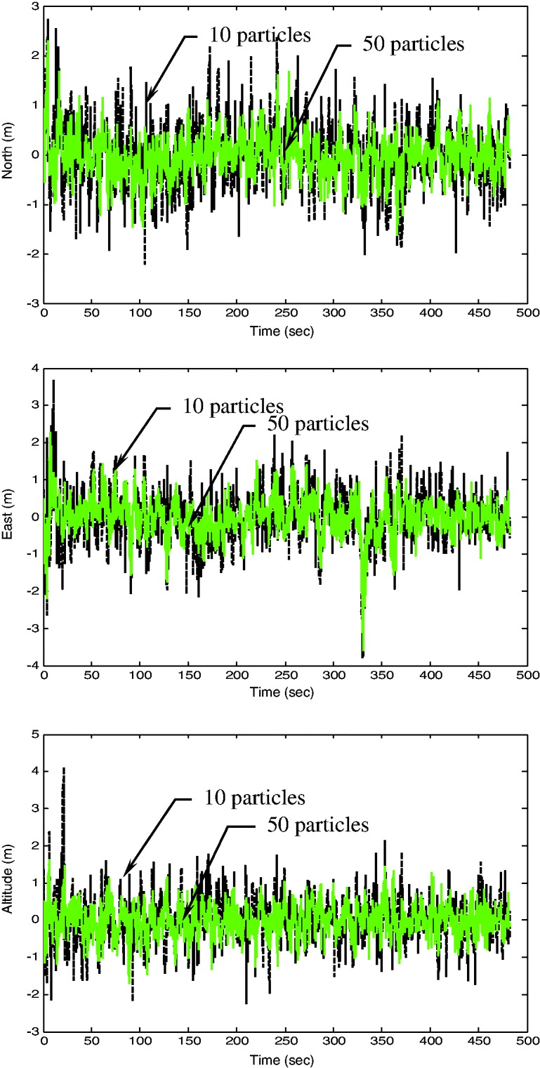
Figure 10. Comparison of position errors for FUPF when 10 and 50 particles are used – Scenario 1 (with aiding).
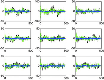
Figure 11. Doppler frequency errors (Hz) for the 9 satellites based on the EKF (black), UKF (green) and FUPF (blue) approaches, all with aiding – Scenario 1.

Figure 12. Comparison of position RMS errors for the five approaches – Scenario 1.
Table 3. Numerical data for the five approaches – Scenario 1 (RMS errors, in metres).
Table 4. Comparison of execution time for various approaches – Scenario 1 (all with aiding, in sec).

Table 5. Comparison of position RMS errors (in metres) for the FUKF with different particle numbers – Scenario 1.

4.2. Scenario 2 (Example 2)
One more example is provided to further confirm the effectiveness and justify the performance of the proposed method. The test trajectory for Example 2 is shown in Figure 13. Table 6 provides description of the vehicle motion. Similarly to Example 1, the trajectory can be divided mainly into ten time intervals/segments according to the dynamic characteristics. The vehicle conducted constant acceleration level flight during 0–12s, clockwise circular motion with radius 275 metres during 50–206s, and counter-clockwise circular motion with radius 250 metres during 271–413s, where high dynamic manoeuvring is involved. For all the other segments, constant-velocity straight-line flight is involved. For Scenario 2, the data for INS error specifications is taken from Crista IMU specifications (2012), as shown in Table 7.
The effectiveness of the proposed method is essentially similar to that obtained in Example 1. Figures 14–16 illustrate the position accuracy for the FUPF as compared to EKF and UKF. The number of particles used in Figure 16 is also 50. It is again verified that, by monitoring the innovation information, the FUPF has good capability to detect the change in vehicle dynamics and tune the scaling factor larger so as to prevent the divergence and retain better navigation accuracy. Figure 17 shows comparison of position errors for FUPF when 10 and 50 particles are used (both with aiding). Doppler frequency errors (Hz) for the 9 satellites based on the EKF (black), UKF (green) and FUPF (blue) approaches are depicted in Figure 18. Furthermore, comparison of position RMS errors for the five approaches is given in Figure 19. Numerical data for the five approaches (RMS errors, in metres) is summarized in Table 8. The FUPF algorithm with Doppler velocity aiding confirms remarkable improvement in navigation estimation accuracy with reduced number of particles. Comparison of execution time for various approaches (with aiding) is given in Table 9. Table 10 provides comparison of position RMS errors for the FUKF when different particle numbers are used.

Figure 13. Three-dimensional test trajectory for Scenario 2.
Table 6. Description of the vehicle motion for Scenario 2.

Table 7. INS error specifications for Scenario 2 (from Crista IMU Specifications [2012]).
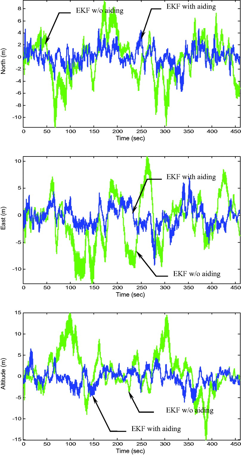
Figure 14. Position errors using the EKF for the cases with aiding and w/o aiding – Scenario 2.

Figure 15. Position errors using the UKF for the cases with aiding and w/o aiding – Scenario 2.

Figure 16. Position errors for FUPF, as compared to the UKF and EKF – Scenario 2 (all with aiding).
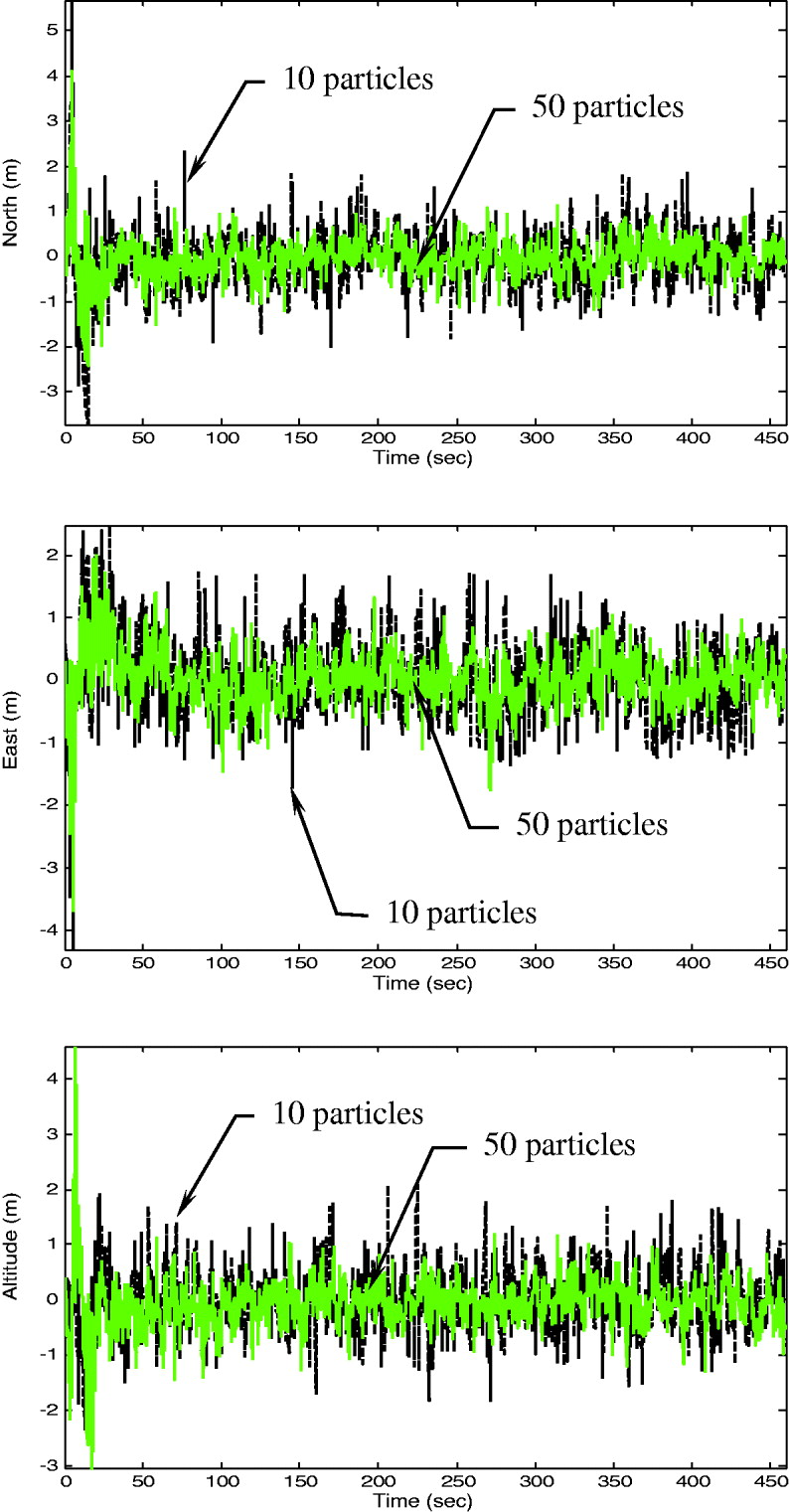
Figure 17. Comparison of position errors for FUPF when 10 and 50 particles are used – Scenario 2 (with aiding).

Figure 18. Doppler frequency errors (Hz) for the 9 satellites based on the EKF (black), UKF (green) and FUPF (blue) approaches, all with aiding – Scenario 2.

Figure 19. Comparison of position RMS errors for the five approaches – Scenario 2.
Table 8. Numerical data for the five approaches – Scenario 2 (RMS errors, in metres).

Table 9. Comparison of execution time for various approaches – Scenario 2 (all with aiding, in sec).

Table 10. Comparison of position RMS errors (in metres) for the FUKF with different particle numbers – Scenario 2.

5. CONCLUSIONS
An alternative state estimation technique called the fuzzy adaptive unscented particle filter has good potential as the state estimation technique for the ultra-tightly coupled Global Positioning System (GPS)/Inertial Navigation System (INS) navigation. One of the principal advantages of the Ultra-Tightly Coupled (UTC) structure is that a Doppler frequency derived from the INS is integrated with the baseband loops to improve the tracking capability of the receiver. The Doppler frequency shift has been calculated and fed to the GPS tracking loops for elimination of the effect of stochastic errors caused by the Doppler frequency. The proposed state estimation technique is designed so as to improve the navigation accuracy at the high dynamic manoeuvring or sharp turning regions while preserving/without sacrificing the precision at the lower dynamic regions. The fuzzy system has been incorporated to improve the assisted Unscented Particle Filter (UPF) performance. As a mechanism for timely detecting the dynamical changes, the Fuzzy Logic Adaptive System (FLAS) implements the on-line tuning of the factors in the weighted covariance matrices by monitoring the innovation information so as to maintain good estimation accuracy and tracking capability.
Simulation studies were carried out for two examples for performance comparison for ultra-integration of GPS and INS. Evaluation of navigation performance among various nonlinear filters, including Extended Kalman Filter (EKF), Unscented Kalman Filter (UKF) and FLAS assisted UPF (FUPF). FUPF for navigation sensor fusion has been presented. As the enhanced version of UPF, the proposed FUPF reveals very promising improvement in navigational accuracy and has very good potential as an alternative navigation state estimator. Nevertheless, selection of the nonlinear filters leads to different levels of computational burden. The UPF requires large computational time as compared to the other algorithms. The FLAS has been incorporated into the UPF for improving the quality of the proposal distribution and therefore reducing the number of particles. The mismatch of the model leads to large navigation error while the FLAS timely detects the increase of Degree Of Divergence (DOD) values, and therefore increases the scaling factor so as to maintain good tracking capability. For trajectories with sharp turns or abrupt manoeuvres involved, the performance improvement becomes obvious. Various numbers of particles were tested. Trade-off needs to be made for selection of a suitable algorithm and numbers of particles for a specific purpose.
The paper justifies the performance for the EKF, UKF, UPF and FUPF methods and confirms the effectiveness of the proposed FUPF method for accuracy improvement especially in the high dynamic environments. The FUPF algorithm with Doppler velocity aiding demonstrates remarkable improvement in navigation estimation accuracy with reduced number of particles.
ACKNOWLEDGEMENTS
This work has been supported in part by the National Science Council of the Republic of China under grant NSC 98-2221-E-019-021-MY3.


