3.1. Resonant triads

As expected, if the basic wave is absent ($\epsilon =0$), the eigenvalue problem (2.9) and (2.12) recovers the free propagating modes in the fluid layer. Specifically, as the coefficients $Q_m$ are entirely uncoupled when $\epsilon =0$, we write

(3.1)\begin{equation} Q_m = q_{m,l}(z;p+m)\quad(l=1,2,\ldots), \end{equation}

for any given $-\infty < m<\infty$, with the rest of the $Q$ being zero. Here, $q_{m,l}$ denote the eigenfunctions of the problem

(3.2a)\begin{gather} \frac{\mathrm{d}^2q_{m,l}}{\mathrm{d}z^2}+ \left(\frac{N^2}{c_{m,l}^2}-(p+m)^2\right)q_{m,l} = 0, \end{gather}

(3.2b)\begin{gather}q_{m,l} = 0 \quad(z=0,H), \end{gather}

and $c_{m,l}^2$ are the corresponding eigenvalues, with

(3.3)\begin{equation} c_{m,l}^2=\frac{\varOmega_m^2}{(p+m)^2}\quad(l=1,2,\ldots). \end{equation}

It should be noted that (3.3) are the dispersion relations of (the countable infinity of) free propagating modes $(l=1,2,\ldots )$, and $\varOmega _m=\pm (p+m)c_{m,l}$ (with $c_{m,l}>0$) are the frequencies (in the rest frame) of these modes at the wavenumber $p+m$. Hence, in view of (2.11), for $\epsilon =0$, the stability eigenvalues $\sigma$ are simply the (Doppler-shifted) frequencies of these waves in the frame moving with $c_n$,

(3.4)\begin{equation} \sigma=\sigma^\pm{\equiv} -(p+m)c_n\pm(p+m)c_{m,l}\quad(l=1,2,\ldots).\end{equation}

Next, we inquire into how the interaction with the underlying wave affects $\sigma$ in the small-amplitude limit ($0<\epsilon \ll 1$). According to (2.9), to leading order in $\epsilon$, each $Q_m$ is coupled to its nearest neighbours $Q_{m\pm 1}$ only. As this coupling is weak, it is natural to attempt to solve the eigenvalue problem (2.9) and (2.12) approximately in an iterative manner, starting from the known solution for $\epsilon =0$ (cf. (3.1)–(3.3)). Specifically, for any given $-\infty < m<\infty$ and $l=1,2,\ldots$, one may anticipate that

(3.5a,b)\begin{equation} Q_m=q_{m,l}(z;p+m)+{O}(\epsilon^2), \quad Q_{m\pm1}=\epsilon \hat{q}_{m\pm1,l}(z)+{O}(\epsilon^2), \end{equation}

with the rest of the $Q$ being smaller than ${O}(\epsilon )$ and

(3.6)\begin{equation} \sigma = \sigma^\pm{+}{O}(\epsilon^2). \end{equation}

Here, $q_{m,l}$ and $\sigma ^\pm$ are the free-mode eigenfunctions and (real) frequencies defined in (3.2) and (3.4), respectively, and the correction terms $\hat {q}_{m\pm 1,l}$ satisfy the forced equations

(3.7a)\begin{equation} \frac{\mathrm{d}^2\hat{q}_{m\pm1,l}}{\mathrm{d}z^2}+(p+m\pm1)^2 \left(\frac{N^2}{\varOmega_{m\pm1}^2}-1\right)\hat{q}_{m\pm1,l} = \frac{1}{2\varOmega_{m\pm1}}\left(K_{m\pm1}^\mp q_{m,l} +D_{m\pm1}^\mp \frac{\mathrm{d}q_{m,l}}{\mathrm{d}z}\right),\end{equation}

subject to the boundary conditions

(3.7b)\begin{equation} \hat{q}_{m\pm1,l} = 0 \quad(z=0,H).\end{equation}

According to (3.5a,b), to leading order, the interaction with the basic wave induces the nearest two neighbours of $Q_m$ to ${O}(\epsilon )$. Furthermore, as indicated by (3.6), no instability is predicted at ${O}(\epsilon )$.

It is important to note, however, that the above (naive) approximation procedure breaks down if $\varOmega _{m\pm 1}^2/(p+m\pm 1)^2$ in (3.7a) happens to coincide with a free-mode eigenvalue (i.e. an eigenvalue $c^2_{m\pm 1,l}$ of the problem (3.2)). Under this resonance condition, which as discussed in the following may be interpreted as two free modes forming a resonant triad with the underlying wave, the forced problems (3.7) generally cannot be solved, and (3.5a,b)–(3.6) need to be revised. Moreover, in this instance it turns out that $\sigma _\mathrm {i}={O}(\epsilon )$, so triad resonances are associated with the onset of instability in the limit $\epsilon \ll 1$.

To analyse this TRI, without loss of generality ($-\infty < p<\infty$ is a free parameter), suppose that $(m=0,l)$ and $(m=1,l+r)$ are resonant free modes, where $l$ and $l+r$ are positive integers. Then, in view of (2.11) and (3.3), the corresponding eigenvalues $c_{0,l}$ and $c_{1,l+r}$ must satisfy

(3.8a)\begin{gather} (\sigma+pc_n)^2=p^2c_{0,l}^2, \end{gather}

(3.8b)\begin{gather}(\sigma+(p+1)c_n)^2=(p+1)^2c_{1,l+r}^2. \end{gather}

Hence,

(3.9)\begin{equation} \pm pc_{0,l}={-}c_n\pm(p+1)c_{1,l+r}, \end{equation}

where the $\pm$ signs above can be chosen independently. Therefore, the wavenumbers $k_0=p$ and $k_1=p+1$, along with the corresponding frequencies (in the rest frame) $\omega _0=\pm pc_{0,l}$ and $\omega _1=\pm (p+1)c_{1,l+r}$ of free modes that satisfy the resonance conditions (3.8), are linked via

(3.10a,b)\begin{equation} k_1-k_0=1,\quad \omega_1\pm\omega_0=c_n. \end{equation}

This confirms that such modes form a resonant triad with the basic wave as the latter has (normalised) wavenumber $1$ and frequency (in the rest frame) $c_n$. Alternatively, in the moving frame where the basic wave has zero frequency, the two resonant free modes have the same frequency, $\sigma$, and the frequency condition in (3.10a,b) is met trivially.

3.2. TRI eigenvalue problem

For given $l$ and $r$, conditions (3.8) determine specific (real) $p=p_c$ and $\sigma =\sigma _c$, say, at which the triad conditions (3.10a,b) are met. (Equation (3.8) may admit multiple such solutions.) Close to these critical values, we write

(3.11a,b)\begin{equation} p=p_c+\hat{p}\epsilon,\quad \sigma=\sigma_c+\lambda\epsilon, \end{equation}

where $\hat {p}$ is a real ${O}(1)$ wavenumber detuning and $\lambda$ is a possibly complex eigenvalue perturbation. In this neighbourhood, we seek solutions of the eigenvalue problem (2.9) and (2.12) in the form

(3.12a)\begin{gather} Q_0 = A_0q_{0,l}(z;p_c)+\epsilon\hat{q}_{0,l}(z) +{O}(\epsilon^2), \end{gather}

(3.12b)\begin{gather}Q_1 = A_1q_{1,l+r}(z;p_c+1)+\epsilon\hat{q}_{1,l+r}(z) +{O}(\epsilon^2), \end{gather}

with $Q_{-1},Q_2={O}(\epsilon )$ and the rest of the $Q$ $\mathscr {o}(\epsilon )$. Here, $q_{0,l}$ and $q_{1,l+r}$ are the eigenfunctions corresponding to the resonant eigenvalues $c_{0,l}$ and $c_{1,l+r}$ of the problem (3.2), under the normalisation

(3.13)\begin{equation} \int_{0}^{H}N^2q_{0,l}^2\, \mathrm{d}z=\int_{0}^{H}N^2q_{1,l+r}^2\, \mathrm{d}z=1,\end{equation}

and $A_0,A_1$ are constants.

Upon substituting (3.12) along with (3.11a,b) in (2.9) and (2.12), the ${O}(1)$ balance of terms is satisfied automatically. Next, the ${O}(\epsilon )$ corrections to $Q_0$ and $Q_1$ in (3.12) are to be found by solving the forced problems

(3.14a)\begin{gather} \frac{\mathrm{d}^2\hat{q}_{0,l}}{\mathrm{d}z^2}+ \left(\frac{N^2}{c_{0,l}^2}-k_0^2\right)\hat{q}_{0,l} = \mathcal{R}_{0,l}, \end{gather}

(3.14b)\begin{gather}\hat{q}_{0,l} = 0 \quad(z=0,H), \end{gather}

and

(3.15a)\begin{gather} \frac{\mathrm{d}^2\hat{q}_{1,l+r}}{\mathrm{d}z^2}+ \left(\frac{N^2}{c_{1,l+r}^2}-k_1^2\right)\hat{q}_{1,l+r} = \mathcal{R}_{1,l+r}, \end{gather}

(3.15b)\begin{gather}\hat{q}_{1,l+r} = 0 \quad(z=0,H). \end{gather}

Here,

(3.16a)\begin{align} \mathcal{R}_{0,l} &=2A_0q_{0,l}\left\{k_0\hat{p}-N^2 \frac{k_0^2}{\omega_0^2}\left(\frac{\hat{p}}{k_0}- \frac{\lambda+c_n\hat{p}}{\omega_0}\right)\right\}\nonumber\\ &\quad+\frac{A_1}{2\omega_0}\left(K_0^+q_{1,l+r}+D_0^+ \frac{\mathrm{d}q_{1,l+r}}{\mathrm{d}z}\right), \end{align}

(3.16b)\begin{align} \mathcal{R}_{1,l+r} &= 2A_1q_{1,l+r}\left\{k_1\hat{p}-N^2 \frac{k_1^2}{\omega_1^2}\left(\frac{\hat{p}}{k_1}-\frac{\lambda +c_n\hat{p}}{\omega_1}\right)\right\}\nonumber\\ &\quad+\frac{A_0}{2\omega_1}\left(K_1^-q_{0,l}+D_1^- \frac{\mathrm{d}q_{0,l}}{\mathrm{d}z}\right), \end{align}

where $k_0=p_c, \omega _0=\sigma _c+c_np_c$ and $k_1=p_c+1$, $\omega _1=\sigma _c+c_n(p_c+1)$ are the resonant triad wavenumbers and frequencies (in the rest frame), and the constants $K_0^+,K_1^-,D_0^+$ and $D_1^-$ are evaluated using (2.10) at $p=p_c$ and $\sigma =\sigma _c$.

Now, similar to the forced problems (3.7), we ask whether the forced problems (3.14) and (3.15) can be solved, given that the corresponding homogeneous problems have non-trivial solutions, namely the eigenfunctions $q_{0,l}(z;p_c)$ and $q_{1,l+r}(z;p_c+1)$, respectively. It turns out that, for (3.14) and (3.15) to be solvable, the forcing terms $\mathcal {R}_{0,l}$ and $\mathcal {R}_{1,l+r}$ must be orthogonal to these homogeneous solutions:

(3.17a,b)\begin{equation} \int_{0}^H\mathcal{R}_{0,l}q_{0,l}\, \mathrm{d}z = 0,\quad \int_{0}^H\mathcal{R}_{1,l+r}q_{1,l+r}\, \mathrm{d}z = 0. \end{equation}

The above solvability conditions are a particular instance of the Fredholm alternative (e.g. Haberman Reference Haberman2012). Here, they are obtained by multiplying both sides of (3.14a) and (3.15a) with $q_{0,l}(z;p_c)$ and $q_{1,l+r}(z;p_c+1)$, respectively, and integrating in $z$ from $0$ to $H$. After two integrations by parts and using the boundary conditions (3.14b) and (3.15b), it follows that the left-hand sides of these equations vanish; thus, the right-hand sides must do so as well, implying (3.17a,b).

Inserting the forcing terms (3.16) in the solvability conditions (3.17a,b) yields the following $2\times 2$ eigenvalue problem for $\lambda$

(3.18a)\begin{gather} (\lambda-c_g^0\hat{p})A_0 = E_1A_1, \end{gather}

(3.18b)\begin{gather}(\lambda-c_g^1\hat{p})A_1 = E_2A_0. \end{gather}

Here, using (2.10), the interaction coefficients $E_1$ and $E_2$ can be brought to the form

(3.19a)\begin{align} E_1 &=\frac{\omega_0^2}{4k_0^2}\left\{(k_1I_1+I_3) \left(\frac{k_1^2}{\omega_1^2}+\frac{k_0k_1}{\omega_0\omega_1}- \frac{k_0}{c_n\omega_0}-\frac{1}{c_n^2}\right)\right.\nonumber\\ &\quad\left.+k_1I_2\left(\frac{k_0}{\omega_0\omega_1}+ \frac{k_1}{\omega_1^2}-\frac{k_0}{c_n\omega_0}- \frac{1}{c_n^2}\right)\right\},\end{align}

(3.19b)\begin{align} E_2 &= \frac{\omega_1^2}{4k_1^2}\left\{(k_0I_1-I_4) \left(\frac{k_0^2}{\omega_0^2}+\frac{k_0k_1}{\omega_0\omega_1}- \frac{k_1}{c_n\omega_1}-\frac{1}{c_n^2}\right)\right.\nonumber\\ &\quad\left.-k_0I_2\left(\frac{k_1}{\omega_0\omega_1}+ \frac{k_0}{\omega_0^2}+\frac{k_1}{c_n\omega_1}+ \frac{1}{c_n^2}\right)\right\}, \end{align}

where the constants $I_1,\ldots,I_4$ are given by

(3.20a)$$\begin{gather} I_1 = \int_{0}^HN^2\bar{f}_n^\prime q_{0,l}q_{1,l+r}\, \mathrm{d}z, \end{gather}$$

(3.20b)$$\begin{gather}I_2 = \int_{0}^H(N^2)^\prime\bar{f}_n q_{0,l}q_{1,l+r}\, \mathrm{d}z, \end{gather}$$

(3.20c)$$\begin{gather}I_3 = \int_{0}^HN^2\bar{f}_n q_{0,l}q_{1,l+r}^\prime\,\mathrm{d}z, \end{gather}$$

(3.20d)$$\begin{gather}I_4 = \int_{0}^HN^2\bar{f}_nq_{0,l}^\prime q_{1,l+r}\, \mathrm{d}z ={-}(I_1+I_2+I_3), \end{gather}$$

with prime denoting derivative with respect to $z$. Finally, the constants $c_g^0$ and $c_g^1$ in (3.18) are associated with the wavenumber detuning in (3.11a,b). From (3.17a,b), also making use of (3.13), these constants can be expressed as

(3.21a)\begin{gather} c_g^0 ={-}c_n+\frac{\omega_0}{k_0}\left(1-\omega_0^2 \int_{0}^Hq_{0,l}^2\, \mathrm{d}z\right), \end{gather}

(3.21b)\begin{gather}c_g^1 ={-}c_n+\frac{\omega_1}{k_1}\left(1-\omega_1^2 \int_{0}^Hq_{1,l+r}^2\, \mathrm{d}z\right), \end{gather}

and they represent the group velocities (in the frame moving with the basic wave) of the modes that form a resonant triad with the basic wave. (Ignoring their interaction with the underlying wave, these modes would be free propagating waves, so a wavenumber shift $\hat {p}\epsilon$ would cause a frequency shift $c_g\hat {p}\epsilon$ in (3.11a,b); i.e. $\lambda =c_g^0\hat {p},c_g^1\hat {p}$, consistent with (3.18) for $E_1=E_2=0$.)

Based on the eigenvalue problem (3.18), instability ($\lambda =\lambda _\mathrm {r}+\mathrm {i}\lambda _\mathrm {i}$ complex) requires $E_1E_2<0$. Moreover, under this condition, instability is present within the ${O}(\epsilon )$ wavenumber window $p=p_c+\hat {p}\epsilon$ specified by

(3.22)\begin{equation} \hat{p}^2 <{-}\frac{4E_1E_2}{(c_g^1-c_g^0)^2}, \end{equation}

with the maximum growth rate

(3.23)\begin{equation} \sigma_{\mathrm{i}}\mid_{max}=\epsilon\lambda_\mathrm{i} \mid_{max}=\epsilon({-}E_1E_2)^{1/2}, \end{equation}

realised at $\hat {p}=0$ $(p=p_c)$.

3.3. The case $N=1$

In the case of uniform background stratification ($N=1$), the eigenfunctions $q_{m,l}$ of the eigenvalue problem (3.2) are sines that depend on the modal number $l$ but not on the wavenumber $p+m$,

(3.24)\begin{equation} q_{m,l} = C\sin\frac{l{\rm \pi}}{H}z\quad(l=1,2,\ldots), \end{equation}

where $C$ is a normalisation constant, and the free-mode dispersion relations (3.3) read

(3.25)\begin{equation} \varOmega_m^2 = \frac{(p+m)^2}{(p+m)^2+(l{\rm \pi}/H)^2}\quad(l=1,2,\ldots). \end{equation}

Thus, the eigenfunctions of possible resonant modes $(m=0,l)$ and $(m=1,l+r)$, under the normalisation (3.13), take the form

(3.26a,b)\begin{equation} q_{0,l} = \left(\frac{2}{H}\right)^{1/2}\sin \frac{l{\rm \pi}}{H}z, \quad q_{1,l+r} = \left(\frac{2}{H}\right)^{1/2} \sin\frac{(l+r){\rm \pi}}{H}z. \end{equation}

Next, based on (3.19) and (3.20), we compute the interaction coefficients $E_1,E_2$ in the TRI eigenvalue problem (3.18). These are linear combinations of $I_1,\ldots,I_4$ and, according to (3.20b), $I_2\equiv 0$ when $N$ is constant. Moreover, using (3.26a,b) and the basic-wave mode (2.7a,b), it follows from (3.20) that the rest of the $I$ vanish as well, unless $r=\pm n$. Thus, in the case of uniform background stratification, TRI requires that perturbations, apart from the resonant triad conditions (3.10a,b), also satisfy

(3.27)\begin{equation} l_1-l_0={\pm} n, \end{equation}

where $n$ is the basic-wave modal number (cf. (2.7a,b)) and $l_0,l_1$ denote the modal numbers of the perturbations. This condition is reminiscent of that satisfied along the vertical by the wavevectors of resonant triads in the TRI of propagating plane waves in an unbounded fluid (e.g. Mied Reference Mied1976). Here, however, the basic state as well as the perturbations are standing waves in the vertical; moreover, in contrast to the triad conditions (3.10a,b), the constraint (3.27) applies only when $N$ is constant. The fact that uniform background stratification limits possible resonant triad interactions of wave modes was also noted by Varma & Mathur (Reference Varma and Mathur2017).

To be specific, we satisfy (3.27) by taking $l_0=l$ and $l_1=l+n$, where $l=1,2,\ldots$. Then, from (3.19), making also use of (2.7a,b), (3.20) and (3.26a,b), we find that

(3.28a)\begin{gather} E_1 = \frac{1}{8n}(nk_0-l)\frac{\omega_0^2}{k_0^2} \left\{\frac{k_1^2}{\omega_1^2}+\frac{k_0k_1}{\omega_0\omega_1}- \frac{k_0}{c_n\omega_0}-\frac{1}{c_n^2}\right\}, \end{gather}

(3.28b)\begin{gather}E_2 = \frac{1}{8n}(nk_0-l)\frac{\omega_1^2}{k_1^2} \left\{\frac{k_0^2}{\omega_0^2}+\frac{k_0k_1}{\omega_0\omega_1}- \frac{k_1}{c_n\omega_1}-\frac{1}{c_n^2}\right\}. \end{gather}

Here, in keeping with (3.10a,b), $k_0=p_c$, $k_1=p_c+1$, $\omega _0=\sigma _c+c_nk_0$ and $\omega _1=\sigma _c+c_nk_1$ are the triad wavenumbers and frequencies, where $p=p_c$ and $\sigma =\sigma _c$ are obtained from the resonance conditions (3.8). In view of (3.25), for $N=1$ these conditions take the form

(3.29a)\begin{gather} \omega_0^2=\frac{p_c^2}{p_c^2+(l{\rm \pi}/H)^2}, \end{gather}

(3.29b)\begin{gather}\omega_1^2=\frac{(p_c+1)^2}{(p_c+1)^2+((l+n){\rm \pi}/H)^2}. \end{gather}

Expressions (3.28) agree with Martin et al. (Reference Martin, Simmons and Wunsch1972) after converting to their non-dimensional variables.

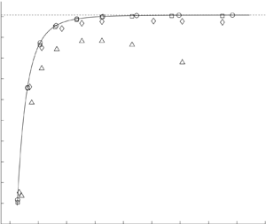
3.4. Comparison with Joubaud et al. (Reference Joubaud, Munroe, Odier and Dauxois2012)

The laboratory experiments of Joubaud et al. (Reference Joubaud, Munroe, Odier and Dauxois2012) employed a wave generator at one end of a uniformly stratified fluid tank to excite monochromatic mode-1 waves which eventually became unstable due to TRI as they propagated along the tank. For each basic wave, Joubaud et al. (Reference Joubaud, Munroe, Odier and Dauxois2012) verified experimentally that the unstable disturbances satisfied the triad resonance conditions and also measured the instability growth rate. Furthermore, they compared the observed TRI growth rates with theoretical estimates based on the TRI of a sinusoidal plane wave in an unbounded fluid.

Here, we make a brief comparison of these observations with the theoretically predicted TRI for mode-1 ($n=1$) waves in a uniformly stratified fluid ($N=1$). Specifically, we focus on the basic wave corresponding to $c_n=0.95$, $H=9.2$ and $\epsilon =0.14$ (in our dimensionless variables), for which Joubaud et al. (Reference Joubaud, Munroe, Odier and Dauxois2012) report the strongest TRI. In this instance, the resonance conditions (3.29) for $l=9$ yield $k_0=1.3$, $\omega _0=-0.39$, $k_1=2.3$ and $\omega _1=0.56$. This resonant triad is a good approximation to the frequencies $\omega _0=-0.38$, $\omega _1=0.57$ as well as the wavenumbers of the observed unstable disturbances in figures 1 and 2 of Joubaud et al. (Reference Joubaud, Munroe, Odier and Dauxois2012). The growth rate found from (3.23) and (3.28) for this triad is $\sigma _\mathrm {i}|_{{theor}}=6.8\times 10^{-2}$ whereas the measured growth rate is $\sigma _\mathrm {i}|_{{exp}}\approx 5.3\times 10^{-2}$. This fair agreement seems reasonable given that the theory does not account for viscous damping so $\sigma _\mathrm {i}|_{theor}$ is expected to overpredict $\sigma _\mathrm {i}|_{exp}$.

4.1. Parametric subharmonic instability

To analyse short-scale instabilities, we introduce a parameter $\mu$ that controls the perturbation vertical length scale and also we scale the horizontal wavenumber $p$ in sympathy with $1/\mu$,

(4.1a,b)\begin{equation} \mu=\frac{H}{{\rm \pi} l},\quad p=\frac{\kappa}{\mu}, \end{equation}

where $\kappa ={O}(1)$ is a re-scaled wavenumber. Thus, conditions (3.29) for determining $p=p_c$ and $\sigma =\sigma _c$ at which the onset of TRI occurs for given $l$, take the form

(4.2a)\begin{gather} \kappa_c^2\left(\frac{1}{\omega_0^2}-1\right)=1, \end{gather}

(4.2b)\begin{gather}(\kappa_c+\mu)^2\left(\frac{1}{\omega_1^2}-1\right)= \left(1+\frac{n{\rm \pi}}{H}\mu\right)^2. \end{gather}

These re-scaled conditions specify $\kappa _c=\mu p_c$ and $\omega _0=\sigma _c+c_np_c$ ($\omega _1=\omega _0+c_n$), for given $\mu$.

In the short-scale limit of interest here, (4.2) are solved by expanding in $\mu \ll 1$

(4.3a)\begin{equation} \kappa_c=\kappa_0+\mu{\rm \Delta}\kappa+\cdots,\quad \omega_0={-}\frac{c_n}{2}+\mu{\rm \Delta}\omega_0+\cdots,\end{equation}

where

(4.3b)\begin{equation} \kappa_0={\pm}\frac{c_n}{(4-c_n^2)^{1/2}},\quad {\rm \Delta} \kappa=\frac{1}{2}\left(\frac{n{\rm \pi}}{H}\kappa_0-1\right),\quad {\rm \Delta}\omega_0={-}\frac{c_n^3}{8\kappa_0^3}{\rm \Delta}\kappa.\end{equation}

Therefore, in this limit, TRI involves two short-scale modes with frequencies (in the rest frame) half the basic-wave frequency: $\omega _0=-c_n/2$ and $\omega _1= c_n/2$. This is the hallmark of the widely studied PSI of sinusoidal plane internal waves and plane wave beams in an unbounded uniformly stratified fluid (Staquet & Sommeria Reference Staquet and Sommeria2002; Dauxois et al. Reference Dauxois, Joubaud, Odier and Venaille2018).

Using (4.3), we may compute asymptotically the interaction coefficients $E_1, E_2$ in (3.28) of the TRI eigenvalue problem (3.18), in the PSI regime. Specifically,

(4.4a)\begin{gather} E_1\sim{-}\frac{1}{16(1-{c_n}^2)^{1/2}} \{(1-c_n^2)^{3/2}\pm(2c_n^2+1)(1-c_n^2/4)^{1/2}\}, \end{gather}

(4.4b)\begin{gather}E_2\sim{-}E_1, \end{gather}

where the $\pm$ sign corresponds to $\kappa _0=\pm c_n/(4-c_n^2)^{1/2}$ in (4.3b). This confirms that $E_1E_2<0$ so, in view of (3.23), PSI is always possible. Furthermore, numerical results (see § 6) indicate that PSI (for the $+$ sign in (4.4), which provides a higher growth rate) is the dominant resonant triad instability.

4.2. Beyond PSI

Recent asymptotic analysis of the Floquet stability eigenvalue problem for internal wave beams (Fan & Akylas Reference Fan and Akylas2021) pointed out that, as the length scale of the perturbation is decreased (for small but fixed beam amplitude), Floquet modes become ‘broadband’: they develop higher-frequency components than the two subharmonics at half the basic wave frequency which are dominant in PSI. This broadening of the frequency spectrum had been noted in earlier numerical work (Onuki & Tanaka Reference Onuki and Tanaka2019) and was attributed to the advection of the perturbation by the underlying wave beam. By adopting a frame riding with the wave beam, Fan & Akylas (Reference Fan and Akylas2021) were able to ‘factor out’ this advection effect and reveal a novel small-scale instability mechanism, distinct from PSI.

Motivated by these findings, we now return to expansion (3.12) and examine the behaviour of the ${O}(\epsilon )$ Fourier coefficients $Q_{-1}$ and $Q_2$ in the short-scale limit ($\mu \ll 1$). It should be noted that, because $\omega _0\sim -c_n/2$ and $\omega _1\sim c_n/2$ in this limit according to (4.3a), these Fourier coefficients are associated with the $\pm 3c_n/2$ frequency components (in the rest frame) of the Floquet mode (2.8).

Specifically, from (2.9) and (2.12) combined with (3.12a), $Q_{-1}$ satisfies the forced equation

(4.5a)\begin{equation} \frac{\mathrm{d}^2Q_{{-}1}}{\mathrm{d}z^2}+(k_0-1)^2 \left(\frac{1}{\varOmega_{{-}1}^2}-1\right)Q_{{-}1}= \epsilon\mathcal{R}_{{-}1}, \end{equation}

subject to

(4.5b)\begin{equation} Q_{{-}1}=0\quad(z=0,H), \end{equation}

where

(4.6)\begin{equation} \mathcal{R}_{{-}1} = \frac{A_0}{2\varOmega_{{-}1}}\left(K_{{-}1}^+q_{0,l}+D_{{-}1}^+ \frac{\mathrm{d}q_{0,l}}{\mathrm{d}z}\right). \end{equation}

In general, the boundary-value problem (4.5) is solvable as $\varOmega _{-1}=\omega _0-c_n$ does not match the frequency of a free mode at the wavenumber $k_{-1}\equiv k_0-1$; i.e. $k_{-1},\varOmega _{-1}$ do not satisfy the dispersion relation (3.25) for any (integer) modal number $l$. Rather than determining the detailed solution, however, here it suffices to look at the asymptotic behaviour of $Q_{-1}$ for $\mu \ll 1$. Briefly, upon combining (2.7a,b), (2.10) and (3.26a,b) with (4.1), (4.3) and $\varOmega _{-1}\sim -3c_n/2$, we find from (4.6)

(4.7)\begin{equation} \mathcal{R}_{{-}1}\sim\frac{16}{9}\frac{A_0}{c_n^3} \left(\frac{2}{H}\right)^{1/2}\frac{\kappa_0^2}{\mu^3} \left\{\kappa_0\cos\frac{n{\rm \pi}}{H}z\sin\frac{z}{\mu}+ \frac{H}{n{\rm \pi}}\sin\frac{n{\rm \pi}}{H}z\cos\frac{z}{\mu}\right\}. \end{equation}

Therefore, the solution of problem (4.5), in the limit $\mu \ll 1$, schematically, takes the form

(4.8)\begin{equation} Q_{{-}1}\sim \frac{\epsilon}{\mu}\left\{A_{{-}1}^+\sin \left(\frac{z}{\mu}+\frac{n{\rm \pi}}{H}z\right)+A_{{-}1}^-\sin \left(\frac{z}{\mu}-\frac{n{\rm \pi}}{H}z\right)\right\}, \end{equation}

where $A^\pm _{-1}$ are certain ${O}(1)$ constants. Thus, $Q_{-1}={O}(\epsilon /\mu )$ and, by a similar procedure, it can be deduced that $Q_2={O}(\epsilon /\mu )$ as well.

The fact that $Q_{-1},Q_2={O}(\epsilon /\mu )$ in the joint limit $\epsilon,\mu \ll 1$ suggests that the coupling of the two resonant free modes in (3.12) with the basic wave, actually is ${O}(\epsilon /\mu )$. Hence, the assumption of weak coupling, which enables these modes to form a resonant triad with the basic wave, is valid when $\mu \gg \epsilon$ only. If this condition is violated (as will be the case for sufficiently fine-scale perturbations), all Fourier coefficients in the Floquet mode (2.8), formally, are expected to be equally important and the disturbance frequency spectrum would be broadband. A similar situation was encountered in the Floquet stability analysis of internal wave beams by Fan & Akylas (Reference Fan and Akylas2021). The treatment of broadband instability of internal wave modes below follows along the lines of this earlier study.

5.1. Streamline coordinates

Returning to the governing equations (2.1), the dominant coupling of the perturbations to the basic wave in the limit $\epsilon,\mu \ll 1$ derives from the Jacobian term in (2.2) which accounts for the advection due to the underlying wave velocity field. This effect can be ‘factored out’ by working with a new set of coordinates, $(x,\,z)\to (\xi,\,\zeta )$, defined by

(5.1a,b)\begin{equation} \xi=x+\frac{1}{c}\int_{}^{x}\bar{\varPsi}_z\,\mathrm{d} x^\prime,\quad\zeta=z-\frac{\bar{\varPsi}}{c}. \end{equation}

It should be noted that the curves $\zeta =\mathrm {constant}$ coincide with the streamlines of the background steady flow $(-c +\bar {\varPsi }_z,-\bar {\varPsi }_x)$, so switching to these ‘streamline coordinates’ is analogous to the change of frame used by Fan & Akylas (Reference Fan and Akylas2021).

For uniform background stratification, in particular, according to (2.5) and (2.7a,b),

(5.2)\begin{equation} \bar{\varPsi}=\epsilon\bar{\psi}\equiv\epsilon \frac{H}{n{\rm \pi}}\sin\frac{n{\rm \pi}}{H}z\cos x, \end{equation}

so the coordinates (5.1a,b) are given by

(5.3a,b)\begin{equation} \xi = x+\frac{\epsilon}{c_n}\cos\frac{n{\rm \pi}}{H}z\sin x, \quad \zeta=z-\frac{\epsilon}{c_n}\frac{H}{n{\rm \pi}}\sin\frac{n{\rm \pi}}{H}z\cos x. \end{equation}

We remark that the basic wave streamfunction $\bar \varPsi$ is $2{\rm \pi}$-periodic in the transformed horizontal coordinate $\xi$, a property that is utilised in the following Floquet stability analysis (see § 5.2). This holds because $\bar \varPsi$ in (5.2) does not involve a term uniform in $x$; i.e. there is no (Eulerian) horizontal mean flow (under more general flow conditions where such a mean flow may be present, the definition of $\xi$ in (5.1a,b) would need to be reconsidered).

Upon implementing the transformation (5.3a,b), the advective derivative (2.2) takes the form

(5.4)\begin{equation} \frac{{\rm D}}{{\rm D}t}\to\frac{\partial}{\partial t} - c_n\frac{\partial}{\partial\xi} +\frac{\epsilon^2}{c_n}\left(\bar{\psi}_z^2- \left(\frac{n{\rm \pi}}{H}\right)^2\bar{\psi}_x^2\right) \frac{\partial}{\partial\xi}. \end{equation}

Thus, the Jacobian term in (2.2) has been eliminated correct to ${O}(\epsilon )$. Furthermore, using (5.2), the ${O}(\epsilon ^2)$ residual is expressed as

(5.5)\begin{equation} \frac{\epsilon^2}{2c_n}\left(\cos2\frac{n{\rm \pi}}{H}\zeta+\cos2\xi\right) \frac{\partial}{\partial\xi}+{O}(\epsilon^3). \end{equation}

The first term represents the advection effect due to the ‘Stokes drift’ (Thorpe Reference Thorpe1968),

(5.6)\begin{equation} \bar{U}^s=\frac{\epsilon^2}{2c_n}\cos2\frac{n{\rm \pi}}{H}\zeta, \end{equation}

which here coincides with the Lagrangian horizontal mean flow associated with the basic wave, because the Eulerian mean flow vanishes. This effect makes an important contribution to the eigenvalue problem governing broadband instability (see § 5.3). The second term in (5.5), by contrast, is relatively insignificant and could have been eliminated by modifying via an ${O}(\epsilon ^2)$ term the definition of $\xi$ in (5.3a,b).

In terms of $\xi$ and $\zeta$, the governing equations (2.1) now read

(5.7a)\begin{align} &\frac{{\rm D}}{{\rm D}t}\nabla^2\psi - \rho_\xi + \frac{\epsilon}{c_n}\left\{\bar{\psi}_z\left(\frac{1}{c_n}\psi-\rho \right)_\xi-\bar{\psi}_x\left(\frac{1}{c_n}\psi-\rho \right)_\zeta\right\}\nonumber\\ &\quad +\frac{\epsilon^2}{c_n^3}\left(\bar{\psi}_z^2- \left(\frac{n{\rm \pi}}{H}\right)^2\bar{\psi}_x^2\right)\psi_\xi = 0, \end{align}

(5.7b)\begin{align} &\frac{{\rm D}}{{\rm D}t}\rho + \psi_\xi -\frac{\epsilon^2}{c_n^2}\left(\bar{\psi}_z^2- \left(\frac{n{\rm \pi}}{H}\right)^2\bar{\psi}_x^2\right) \psi_\xi = 0, \end{align}

where

(5.8)\begin{align} &\nabla^2 \to \left(1+\frac{\epsilon}{c_n}\bar{\psi}_z\right)^2 \frac{\partial^2}{\partial\xi^2}+\left(1- \frac{\epsilon}{c_n}\bar{\psi}_z\right)^2\frac{\partial^2}{\partial \zeta^2}\nonumber\\ &\quad +2\frac{\epsilon}{c_n}\bar{\psi}_x \left(\left(\frac{n{\rm \pi}}{H}\right)^2-1- \frac{\epsilon}{c_n^3}\bar{\psi}_z\right) \frac{\partial^2}{\partial\xi\partial\zeta}+ \frac{\epsilon}{c_n^3}\left(\bar{\psi}\frac{\partial}{\partial\zeta} +\bar{\psi}_{xz}\frac{\partial}{\partial\xi}\right)\nonumber\\ &\quad +\frac{\epsilon^2}{c_n^2}\bar{\psi}_x^2 \left(\frac{\partial^2}{\partial\zeta^2}+\left(\frac{n{\rm \pi}}{H} \right)^4\frac{\partial^2}{\partial\xi^2}\right). \end{align}

In addition, as the channel walls $z=0,H$ correspond to the streamlines $\zeta =0,H$, the boundary conditions (2.3) translate into

(5.9)\begin{equation} \psi_\xi=0\quad(\zeta=0,H). \end{equation}

5.2. Floquet stability analysis

As the coefficients of the transformed equations (5.7) are steady in $t$ and $2{\rm \pi}$-periodic in $\xi$, we seek Floquet-mode solutions similar to (2.8),

(5.10)\begin{equation} (\psi,\rho) = \mathrm{e}^{-\mathrm{i}\sigma t}\mathrm{e}^{\mathrm{i} p\xi}\sum_{m={-}\infty}^{\infty}\left(\tilde{Q}_m(\zeta), \tilde{R}_m(\zeta)\right)\mathrm{e}^{\mathrm{i}m\xi}, \end{equation}

where the Fourier coefficients $\tilde {Q}_m, \tilde {R}_m$ $(-\infty < m<\infty )$ and the eigenvalue $\sigma$ are to be determined.

Here, our interest is on short-scale perturbations $(\mu \ll 1)$ in the regime

(5.11)\begin{equation} \alpha\equiv\frac{\mu}{\epsilon}={O}(1), \end{equation}

where, as argued in § 4.2, PSI is replaced by a broadband instability. To analyse this ‘distinguished limit’, we work with the scaled wavenumber $\kappa =p\mu ={O}(1)$ defined in (4.1a,b) and the ‘stretched’ coordinate

(5.12)\begin{equation} Z=\frac{\zeta}{\mu}. \end{equation}

Furthermore, we re-scale $\tilde {Q}_m\to \mu \tilde {Q}_m\ (Z,\zeta )$ so that

(5.13)\begin{equation} \frac{\mathrm{d}\tilde{Q}_m}{\mathrm{d}\zeta}\to \frac{\partial\tilde{Q}_m}{\partial Z}+\mu\frac{\partial\tilde{Q}_m}{\partial\zeta}. \end{equation}

It should be noted that, in view of the transformation (5.3a,b), $\exp (\mathrm {i}p\xi )$ in (5.10) involves all harmonics in $x$. Moreover, for $p={O}(1/\mu )$ and $\epsilon /\mu ={O}(1)$ these harmonics contribute at the same level. Thus, in the regime (5.11) the modes (5.10) are ‘broadband’ even though, as discussed below, the $m=0,1$ components are dominant in the Fourier series in $\xi$.

Now, we derive the equations governing $\tilde {R}_m,\tilde {Q}_m$ and $\sigma$ by substituting (5.10) in (5.7) and implementing the scalings (5.11)–(5.13). Specifically, also making use of (5.5), (5.7b) yields correct to ${O}(\epsilon )$

(5.14)\begin{align} \varOmega_m\tilde{R}_m&= \kappa\tilde{Q}_m+\epsilon \left\{\alpha m+\frac{\kappa^2}{2\alpha c_n\varOmega_m}\cos2 \frac{n{\rm \pi}}{H}\zeta\right\}\tilde{Q}_m\nonumber\\ &\quad + \epsilon\frac{\kappa^2}{4\alpha c_n} \left\{\frac{\tilde{Q}_{m+2}}{\varOmega_{m+2}}+ \frac{\tilde{Q}_{m-2}}{\varOmega_{m-2}}\right\}, \end{align}

where $\varOmega _m$ is given in (2.11). Next, using (5.5), (5.8) and upon eliminating $\tilde {R}_m$ via (5.14), we obtain from (5.7a) the following equation system for $\tilde {Q}_m$ $(-\infty < m<\infty )$ correct to ${O}(\epsilon )$

(5.15) \begin{align} &\left\{\left(\frac{\partial}{\partial Z}+\alpha\epsilon \frac{\partial}{\partial\zeta}\right)^2+ (\kappa+\alpha m\epsilon)^2\left(\frac{1}{\varOmega_m^2}-1 \right)\right\}\tilde{Q}_m\nonumber\\ &\quad +\epsilon\left\{\vphantom{\left(H^+_m\frac{\partial\tilde{Q}_{m+1}}{\partial Z}-H^-_m \frac{\partial\tilde{Q}_{m-1}}{\partial Z}\right)}\cos2\frac{n{\rm \pi}}{H}\zeta G_m \tilde{Q}_m-\cos\frac{n{\rm \pi}}{H}\zeta(G^+_m\tilde{Q}_{m+1} +G^-_m\tilde{Q}_{m-1})\right.\nonumber\\ &\quad\left.+\sin\frac{n{\rm \pi}}{H}\zeta \left(H^+_m\frac{\partial\tilde{Q}_{m+1}}{\partial Z}-H^-_m \frac{\partial\tilde{Q}_{m-1}}{\partial Z}\right)+ L^+_m\tilde{Q}_{m+2}+L^-_m\tilde{Q}_{m-2}\right\}=0, \end{align}

where

(5.16a)\begin{gather} G_m= \frac{\kappa^3}{\alpha c_n\varOmega_m^3}, \end{gather}

(5.16b)\begin{gather}G_m^\pm{=} \frac{\kappa^2}{c_n}\left(2-\frac{1}{\varOmega_{m\pm1}^2}- \frac{1}{2\varOmega_m\varOmega_{m\pm1}}\right), \end{gather}

(5.16c)\begin{gather}H_m^\pm{=} \frac{\kappa}{c_n}\left(\frac{H}{n{\rm \pi}}\right) \left(\left(\frac{n{\rm \pi}}{H}\right)^2-1+\frac{1}{2\varOmega_m \varOmega_{m\pm1}}\right), \end{gather}

(5.16d)\begin{gather}L_m^\pm{=} \frac{\kappa^3}{4\alpha c_n\varOmega_m \varOmega_{m\pm2}}\left(\frac{1}{\varOmega_m}+ \frac{1}{\varOmega_{m\pm2}}\right). \end{gather}

5.3. Eigenvalue problem for $\alpha ={O}(1)$

Using the equation system (5.15), we now derive the stability eigenvalue problem appropriate to the asymptotic regime (5.11). To this end, $\kappa$ and $\varOmega _0$ are assumed to be in the vicinity of the critical values $\kappa =\kappa _c$ and $\varOmega _0=\omega _0$ in (4.3) where the triad resonance conditions (4.2) are met for $\mu \ll 1$. Accordingly, we write

(5.17)\begin{equation} \kappa = \kappa_0 + (\alpha{\rm \Delta}\kappa+s)\epsilon,\quad \varOmega_0={-}\frac{c_n}{2}+(\alpha{\rm \Delta}\omega_0+\lambda)\epsilon, \end{equation}

where $\kappa _0$, ${\rm \Delta} \kappa$ and ${\rm \Delta} \omega _0$ are given in (4.3b), $s={O}(1)$ is a real wavenumber detuning and $\lambda$ is a generally complex eigenvalue to be determined. It should be noted that, because $\mu =\alpha \epsilon$ according to (5.11), the ${O}(\alpha \epsilon )$ terms in (5.17) are the ${O}(\mu )$ corrections to $\kappa _c$ and $\omega _0$ in (4.3a). The eigenvalue $\lambda$ hinges on the detuning $s$ and, more importantly, the resonant interaction of perturbations with the basic wave, which can cause instability.

For $\kappa$, $\varOmega _0$ and $\varOmega _1=\varOmega _0+c_n$ in keeping with (5.17), the solution of (5.15) consistent with the boundary conditions (5.9) takes the form

(5.18a)\begin{gather} \tilde{Q}_0=\sum_{r={-}\infty}^\infty A_{0,r}\sin \left(Z+\frac{r{\rm \pi}}{H}\zeta\right)+{O}(\epsilon^2), \end{gather}

(5.18b)\begin{gather}\tilde{Q}_1=\sum_{r={-}\infty}^\infty A_{1,r}\sin \left(Z+\frac{r{\rm \pi}}{H}\zeta\right)+{O}(\epsilon^2), \end{gather}

with the rest of $\tilde {Q}_m(m\neq 0,1){O}(\epsilon )$ or smaller. The coefficients $A_{0,r}$ and $A_{1,r}$ $(-\infty < r<\infty )$ are determined by substituting (5.18) in (5.15) for $m=0,1$ and collecting terms proportional to $\sin (Z+({r{\rm \pi} }/{H})\zeta )$ correct to ${O}(\epsilon )$. Specifically, making also use of (5.16) and (5.17), we find

(5.19a)\begin{align} &\left\{\lambda\pm s(1-c_n^2/4)^{3/2}-\frac{\alpha}{2} \frac{r{\rm \pi}}{H}c_n(1-c_n^2/4)\right\}A_0,r \nonumber\\ &\quad = \tilde{E}^\pm A_{1,r+n}+\tilde{E}^\mp A_{1,r-n}\pm \frac{\tilde{D}}{\alpha}(A_{0,r-2n}+A_{0,r+2n}), \end{align}

(5.19b)\begin{align} &\left\{\lambda\mp s(1-c_n^2/4)^{3/2}+\frac{\alpha}{2} \frac{(r-n){\rm \pi}}{H}c_n(1-c_n^2/4)\right\}A_1,r \nonumber\\ &\quad ={-}\tilde{E}^\mp A_{0,r+n}-\tilde{E}^\pm A_{0,r-n}\pm \frac{\tilde{D}}{\alpha}(A_{1,r-2n}+A_{1,r+2n}). \end{align}

Here

(5.20a)\begin{gather} \tilde{E}^\pm{=}{-}\frac{1}{16(1-{c_n}^2)^{1/2}} \{(1-c_n^2)^{3/2}\pm(2c_n^2+1)(1-c_n^2/4)^{1/2}\}, \end{gather}

(5.20b)\begin{gather}\tilde{D}= \frac{1}{8(1-c_n^2/4)^{1/2}}, \end{gather}

where the upper (lower) sign in (5.19) and (5.20) corresponds to the positive (negative) value of $\kappa _0$ in (4.3b).

The equation system (5.19) is the desired stability eigenvalue problem for short-scale perturbations $(\mu \ll 1)$ in the broadband regime $\mu ={O}(\epsilon )$. This problem, in contrast to the $2\times 2$ system (3.18) that governs TRI, formally involves infinite number of mode amplitudes $A_{0,r}$ and $A_{1,r}$ ($-\infty < r<\infty$): when $\mu ={O}(\epsilon )$ all modes with wavenumber $k_0\sim \kappa _0/\mu (k_1=k_0+1)$ and modal number $(H/{\rm \pi} )/\mu +r$ are nearly resonant and participate in the interaction with the basic wave. Of particular note are the interaction terms proportional to $\tilde {D}/\alpha$ in the system (5.19); in view of (5.20b) and (4.3b), $\pm \tilde {D}/\alpha =k_0\epsilon /4c_n$ so these terms arise from the ‘Doppler shift’ $k_0\bar {U}^s$ of the perturbations by the Stokes drift $\bar {U}^s$ in (5.6).

Finally, as expected when $\epsilon \ll \mu \ll 1(\alpha \gg 1)$, the broadband instability eigenvalue problem (5.19) reduces to the PSI limit of the TRI eigenvalue problem (3.18). Specifically, in the limit $\alpha \gg 1$, $A_{0,0}$ and $A_{1,n}$ dominate the rest of the amplitudes, so (5.19) simplifies to

(5.21a)\begin{gather} \{\lambda\pm s(1-c_n^2/4)^{3/2}\}A_{0,0}=\tilde{E}^\pm A_{1,n}, \end{gather}

(5.21b)\begin{gather}\{\lambda\mp s(1-c_n^2/4)^{3/2}\}A_{1,n}={-}\tilde{E}^\pm A_{0,0}. \end{gather}

Returning to (5.20a) and noting that $\tilde {E}^\pm$ and $-\tilde {E}^\pm$ match the asymptotic expressions (4.4) for the TRI interaction coefficients $E_1$ and $E_2$, respectively, the $2\times 2$ eigenvalue problem (5.21) agrees with (3.18) in the PSI limit.