


1. Introduction
The Gerstner (Reference Gerstner1809) waves, with circular particle orbits, and the Miche (Reference Miche1944) modification to finite depth and elliptic orbits, were extended to irregular, random Lagrange waves by Pierson (Reference Pierson1961). The works by Cieślikiewicz & Gudmestad (Reference Cieślikiewicz and Gudmestad1995) and Gjøsund (Reference Gjøsund2003) are early examples of systematic studies of the kinematics of such waves.
The particle orbits, and their mathematical equivalents, their velocities, have been studied intensely in recent years. Ehrnström & Villari (Reference Ehrnström and Villari2009) give an overview of some of the mathematical aspects from a deterministic viewpoint. Pure empirical studies on orbits in ocean waves are scarce owing to the difficulty and cost of obtaining accurate data, even with modern techniques (Romero & Melville Reference Romero and Melville2010; Fedele et al. Reference Fedele, Benetazzo, Gallego, Shih, Yezzi, Barbaroi and Ardhuin2013; Benetazzo et al. Reference Benetazzo, Bergamasco, Yoo, Cavalieri, Kim, Berotti, Barbariol and Shim2018). Most orbital studies are therefore performed in combination with experiments in a physical or numerical wave tank.
The following studies are of high relevance for the present work. Chen, Hsu & Chen (Reference Chen, Hsu and Chen2010) and Chen et al. (Reference Chen, Li, Hsu and Ng2012) analyse theoretical Lagrangian models for monochromatic waves over uniform and sloping bottoms and compare particle orbits with experimental results. Grue & Jensen (Reference Grue and Jensen2012) and Grue & Kolaas (Reference Grue and Kolaas2017) report particle velocities for both laboratory waves and directional ocean waves based on Romero & Melville (Reference Romero and Melville2010) and reconstruct the orbits with respect to different phases and vertical positions. Starting with the ‘Choppy wave’ model Nouguier, Guérin & Chapron (Reference Nouguier, Guérin and Chapron2009), Nouguier, Chapron & Guérin (Reference Nouguier, Chapron and Guérin2015) and Guérin et al. (Reference Guérin, Desmars, Grilli, Ducrozet, Perignon and Ferrant2019) improve on the Lagrange model for semi-regular and irregular waves with consequences for particle orbit studies. Creamer et al. (Reference Creamer, Henyey, Schult and Wright1989) give an alternative to the second-order technique in the cited works. Experimental studies by van den Bremer et al. (Reference van den Bremer, Whittaker, Calvert, Raby and Taylor2019) on monochromatic waves focus on mass transport and particle orbits at different depths near wave crests and wave troughs, respectively.
We shall investigate systematic and statistical relations between the degree of front–back asymmetry of individual waves in space and time and the geometry of particle orbits. From a statistical viewpoint one may call the former property an apparent (Euler) characteristic, and the latter an intrinsic (Lagrangian) characteristic. The dominant way to empirically describe a sea state is by its energy spectrum, a typical Eulerian concept. The stochastic connection with a Lagrangian description goes via hydrodynamic equations of varying complexity. In this work we will use Gaussian stochastic models for the Lagrangian vertical and horizontal movements and numerically transform them to an Euler description of the water surface. The link between the two descriptions is described, e.g. in Lindgren & Lindgren (Reference Lindgren and Lindgren2011) and Guérin et al. (Reference Guérin, Desmars, Grilli, Ducrozet, Perignon and Ferrant2019). We study unidirectional irregular waves developing in time and space along a straight line over constant depth  $h$.
$h$.
To finish this introduction we make a comment on the photographs taken by Wallet & Ruellan (Reference Wallet and Ruellan1950) on particle trajectories in plane water waves reflected by a partially absorbing barrier, reproduced in Hutter, Wang & Chubarenko (Reference Hutter, Wang and Chubarenko2011, figure 7.8). For a monochromatic wave without reflection the trajectories are very regular in intermediate water, nearly circles at the surface and elliptical near the bottom. With increasing moderate reflection the reflected wave will interfere with the forward travelling wave with increased irregularity and orientation as the result. In the present work the irregularity will come from a continuum of frequencies resulting in a statistical distribution for the trajectories including a statistical relation with the wave asymmetry.
2. The Gauss–Lagrange models
The theme in this paper is the relation between individual wave front–back asymmetry and the shape and orientation of water particle orbits. The idea is that the relation is an inherent relation, appearing in all theoretical models for irregular waves. The model chosen is the first-order Gauss–Lagrange model, and its second-order extension.
2.1. The free and forced first-order models
The first-order Gauss–Lagrange two-dimensional wave model is defined by two correlated Gaussian space–time random fields, describing the vertical and horizontal particle positions as functions of time  $t$ and original horizontal position $u$ along the horizontal axis. Together, these fields define the orbital movements of the water particles. We consider here only particles at the free surface but the model extends to general depth. Following Pierson (Reference Pierson1961), the energy spectrum $S(\omega )$ of the vertical field is called the orbital spectrum. It is not identical to the Euler spectrum, obtained from observations of the ocean surface, but the difference is of no relevance in the present work.
Representing the continuous energy spectrum by a spectrum over discrete frequencies  $\omega _j =j \Delta \omega$ and wavenumbers $k_j$, we write the models for particles on the free surface as
 \begin{gather} \text{vertical position} : W(u,t) = \sum_j A_j \cos (k_j u - \omega_j t - \phi_j), \end{gather}
 \begin{gather}\text{horizontal position} : X(u,t) = u + \sum_j A_j h_j \cos (k_j u - \omega_j t - \phi_j +{\rm \pi}/2). \end{gather}
Here,  $h_j = \cosh (k_j h)/\sinh (k_j h)$ is the depth dependent amplitude factor, with dispersion relation $\omega _j = \sqrt {gk_j \tanh (k_jh)}$. The amplitudes $A_j$ can be taken as deterministic, $A_j = \sqrt {2 S(\omega _j) \Delta \omega }$, but to obtain correct variability in the simulations we must let them be random, $A_j = \sqrt {a_j^{2} + b_j^{2}}$, with independent normal variables $a_j, b_j$, with mean zero and equal variance such that $A_j^{2}$ has expected value $2 S(\omega _j) \Delta \omega$. The relative phases $\phi _j$ shall be independent and uniformly distributed in $[0 , 2{\rm \pi} ]$, and the phase shift between vertical and horizontal movement is ${\rm \pi} /2$ as in (2.2), independent of frequency.
As was shown in Lindgren & Åberg (Reference Lindgren and Åberg2009) and Lindgren (Reference Lindgren2010) the Lagrange model with constant phase shift (2.2) will produce waves which are statistically symmetric with respect to wave front and wave back slopes. To get statistically asymmetric waves one can modify (2.2) and introduce a frequency dependent phase shift  $\rho _j$,
 \begin{equation} \text{horizontal position} : X_{mod}(u,t) = u + \sum_j A_j h_j \cos (k_j u - \omega_j t - \phi_j +\rho_j). \end{equation}
A heuristic choice, inspired by the filtering equation
 \begin{equation} \partial^{2} X_{mod}/\partial t^{2} = \partial^{2} X/\partial t^{2} + a W \end{equation}
and not underpinned by hydrodynamic theory, leads to
 \begin{equation} h_j \exp (\mathrm{i}\rho_j) = \mathrm{i} \cosh (k_j h)/\sinh(k_j h) -a/\omega_j^{2}, \end{equation}
where the  $a$-value determines the degree of statistical wave asymmetry. The model can be used to reproduce statistical asymmetry that can be observed in real ocean waves.
From the pair  $W(u,t), X(u,t)$ one can implicitly define a Lagrange wave $L(x,t)$ by
 \begin{equation} L(X(u,t),t) = W(u,t), \end{equation}
that is, its surface height at time  $t$ at location $X(u,t)$ is $W(u,t)$. We call the Lagrange model defined by (2.2) and constant phase shift the free Lagrange model and the one defined by (2.3) the model with forced asymmetry, which will be dealt with in § 4.3.
2.2. The second-order model
In the second-order Lagrange model the independent frequency components in (2.1) and (2.2) are combined over pairs of frequencies to give second-order terms, added to the first-order terms. This model exists in many different versions and we present here only the simplest form for the vertical process as an example
 \begin{equation} W_2 (0,t) = \mathrm{Re} \sum Z_j Z_k \, H_{jk}^{+} \exp({\mathrm{i}(\omega_j + \omega_k) t}) + \mathrm{Re} \sum Z_j Z_k^{*} \, H_{jk}^{-} \exp({\mathrm{i}(\omega_j - \omega_k) t}). \end{equation}
Here,  $Z_j = a_j+\mathrm {i} b_j$ are the complex representations of the first-order amplitudes and $H_{jk}^{+}, H_{jk}^{-}$ are complex depth and frequency dependent transfer factors; for examples see Marthinsen & Winterstein (Reference Marthinsen, Winterstein, Chung, Isaacson and Maeda1992), Fouques, Krogstad & Myhaug (Reference Fouques, Krogstad and Myhaug2006), Nouguier et al. (Reference Nouguier, Chapron and Guérin2015) and Herbers & Janssen (Reference Herbers and Janssen2016).
When the sum of first- and second-order terms are combined in (2.6) we get the second-order Lagrange model. That model has recently been studied by Guérin et al. (Reference Guérin, Desmars, Grilli, Ducrozet, Perignon and Ferrant2019), whose theoretical results have bearing also on the particle orbits. To complement their theoretical studies we will simulate the relation between wave asymmetry and orbits in the second-order model and then use the formulation by Biésel (Reference Biésel1952) to generate the second-order corrections  $W_2(u,t), X_2(u,t)$. The routine is implemented in the Matlab package WAFO and is described in Lindgren & Prevosto (Reference Lindgren and Prevosto2017). The routine also gives the stochastic local Stokes drift $X_{2,drift}(u,t)$. In the simulations we will use the average Stokes drift from the integral formula, $\int k \omega S(\omega )\, \mathrm {d} \omega$.
2.3. Wave asymmetry and particle orbits
The themes in this paper are the systematic and statistical relations between the degree of front–back asymmetry of irregular random waves, and the shape and orientation of the associated particle orbits. For that reason we make the following definitions of the asymmetry of individual waves, different from those used by, among others, Stansell, Wolfram & Zachary (Reference Stansell, Wolfram and Zachary2003).
For time waves we record the free surface height variation at a fixed location, and identify the sequence of local maxima and minima in the recording. By an individual time wave we mean the part of the signal that lies between two successive local minima. Its front and back slopes are defined as the rate of increase from the initial minimum to the maximum and the rate of decrease from the maximum to the terminal minimum, respectively. As measure of asymmetry we take the logarithm of the ratio between the two. A positive skewness measure means a fast increase and slow decrease.
For space waves we record the surface variation along a straight line at a fixed time. Identifying local minima and maxima we compute front and back slopes, with the front facing the direction towards which waves are travelling. A positive logarithmic skewness measure means a steep front.
For orbit shape and orientation we will study the particle that is located at the maximum of each individual wave in time or space, at the time of observation. This means that we follow that particle in a time interval before and after the time point when the maximum was registered. The orbit is approximated by an ellipse and the direction of its major axis identified. We choose clockwise orientation for both time and space wave orbits, which is consistent with the assumed main wave direction.
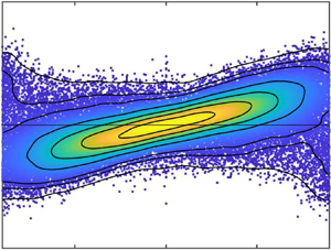
Figure 1 illustrates the skewness–orbit relation. Figure 1(a) shows individual time waves with positive skewness and figure 1(b) shows the orbits for the particles at the wave maxima; the orbits were observed over the time interval between the two nearest local minima. Figures 1(c) and 1(d) show the relation for negatively skewed waves. The orbit tilt/skewness probability density function (p.d.f.) is based on almost 100 000 pairs with observed wave skewness measure and orbit tilt measure. Only waves with a maximum exceeding half the standard deviation and sufficient amplitudes are represented in the figures. The wave model is a first-order model with a Pierson–Moskowitz (PM) orbital spectrum with  $H_s = 4.5\ \textrm {m}$ and $T_p = 10\ \textrm {s}$ at infinite depth.

Figure 1. Illustration of the results of the study. Panels (a,c) show the shape of individual time waves during a 200 s observation period, with positive  $(a)$ and negative $(c)$ skewness. Panels (b,d) show the orbits of the top particle for the respective waves. The black dots indicate the orbit maximum value. The blue circles and red crosses represent the particle locations at the local orbit minima before and after the maximum. Only waves with maximum height at least $H_s/8$ and at least $H_s/4$ front and back amplitudes are represented in the figures. $(e)$ Orbit tilt/skewness scatter plot shows the bivariate distribution of orbit tilt and wave skewness observed in 1000 independent replicates of two hour observation periods. The black level curves enclose areas that contain 10 %, 30 %, 50 %, 70 %, 90 %, 95 %, 99 % of data. The empirical distribution (p.d.f.) to the right illustrates the relation between orbit tilt and wave asymmetry in time waves with Pierson–Moskowitz (PM) orbital spectrum with $H_s = 4.5\ \textrm {m}$ and $T_p = 10\ \textrm {s}$ at infinite depth.
Figure 2 illustrates the wave shape/orbit relation for space wave in the same sea state as in figure 1. We will compare time and space waves systematically in § 4.1.

Figure 2. Wave shapes and orbits from a 3 km space wave sampled at 0.5 m distance, with positive skewness in (a,b) and negative in (c,d), and joint p.d.f. from nearly 24 000 pairs of tilt and skewness from PM space waves at infinite depth.
3. Method
It will be shown by simulation that there exist strong relations between wave skewness and orbital orientation, both for models with statistically symmetric first-order waves, (2.2), and for models with different types of wave asymmetry, including second-order waves with and without a Stokes drift, and waves with forced statistical asymmetry, (2.3).
For a pre-defined orbital spectrum  $S(\omega ), \omega > 0$, we shall generate independent realizations of the vertical $W(u,t)$ and horizontal $X(u,t)$ components in the Gauss–Lagrange model along a line $0 \leq u \leq U$ for a time span $0 \leq t \leq T$, in a discrete space and time grid, $u_n = n\Delta u, t_m = m \Delta t$. In the simulation experiments we will use the routine spec2ldat3DM (Lindgren & Prevosto Reference Lindgren and Prevosto2017) in the module lagrange in the Matlab toolbox WAFO (WAFO-group 2017).
If  $X(u,t)$ is a strictly increasing function of $u$ then (2.6) has a unique solution $L(x,t)$ for $t \in [0,T]$ and $x$ in some common (random) interval, $x \in [x_{min}, x_{max}]$. Keeping $t=t_0$ fixed we obtain a Lagrange space wave $L(u,t_0)$ and keeping $x = x_0$ fixed we obtain a time wave $L(x_0,t)$. As noted already by Pierson (Reference Pierson1961) it can happen that $X(u,t)$ is not strictly increasing but for the sea states and water depths we consider in the paper these events are very rare.
For each wave realization we identify all local maxima and minima and the corresponding front and back steepnesses. Simultaneously computing the particle orbits from the model, we can find a pair ‘before–after asymmetry – orbit shape and orientation’ for each local maximum. The procedure is repeated with independent realizations, and it will give an estimate of the statistical relation between wave asymmetry and orbit orientation. Details on the sampling procedure to obtain individual waves and on the different measures will be given in §§ 3.1 and 3.2.
As an alternative to the min/max definition one can take the trough/crest definition, where the wave is defined by the maximum and minimum between successive zero crossings. This will lead to more chaotic orbits with extra twists and less characteristic skewness measures. The link between tilt and skewness will be weaker but still significant.
3.1. Space waves
For space waves we fix a time point  $t_0$ and observe maxima and minima, $M_k$, $m_k$, in $L(x,t_0)$ as a function of $x$. We denote their locations by $x^{+}_k, x^{-}_k$ with the wave front facing the positive $x$-direction and define the front and back steepnesses by
 \begin{equation} \left. \begin{gathered} s_k^{+} = (M_k - m_{k+1})/(x_k^{+}-x_{k+1}^{-})<0,\\ s_k^{-} = (M_k - m_k)/(x_k^{+}-x_k^{-})>0. \end{gathered} \right\} \end{equation}
The front–back asymmetry is recorded in logarithmic scale as  $A_k = \log (-s_k^{+}/s_{k}^{-})$ and waves with positive $A_k$ have a steep front and less steep back; see figure 3 for an illustration.

Figure 3. A space wave moving from left to right and its top particle orbit (blue) with the fitted ellipse (red).  $(a)$ A space wave with positive skewness; dot marks the maximum of the wave. $(b)$ Orbit of the particle at the wave maximum; dot marks the maximum of the orbit. Note that the orbit maximum comes approximately 0.3 s after the registration of the wave. Circles and cross indicate the starting and final minima of the wave and the orbit, respectively.
To find the trajectory of the particle that is located at the maximum  $M_k$ we observe that, when $X(u,t_0)$ is strictly increasing, which is the case in all the examples, for each $k$ there is a unique origin $\tilde {u}_k$ such that $X(\tilde {u}_k,t_0) = x_k^{+}$, and hence $W(\tilde {u}_k, t_0) = M_k$. The centred trajectory of the top particle therefore has coordinates, as a function of $\tau$,
 \begin{equation} O_k(\tau) = \{X(\tilde{u}_k, t_0 + \tau)-{\tilde{u}_k}, W(\tilde{u}_k, t_0 + \tau)\}, \; -d_k^{-} \leq \tau \leq d_k^{+}. \end{equation}
 The time interval for the orbit of the top particle will be defined by its movement before and after the observation time point  $t_0$, as follows. For the maximum at $x_k^{+}$, originating from position $\tilde {u}_k$ we define $d_k^{\pm }$ so that $W(\tilde {u}_k, t_0 + \tau )$ has local minima for $t_0-d_k^{-}$ and $t_0+d_k^{+}$, these minima being the closest to $t_0$. This definition works well if the maximum $M_k$ is sufficiently high. It is less suitable for very low maxima for which other methods are needed for an analysis of the orbit–asymmetry relation.
3.2. Time waves
For time waves we fix an observation point  $x_0 \in [x_{min}, x_{max}]$, and observe the surface variation $L(x_0,t)$ at that point, identifying all local maxima and minima in that time series, and the corresponding front and back steepnesses.
In each realization, we denote the height of local maxima in  $L(x_0,t)$ by $M_k, k=1,\ldots ,n$ and their time of occurrence by $t_k^{+}$. We denote the height of the preceding and following local minima by $m_k, m_{k+1}$ and let their time of occurrence be $t_k^{-}, t_{k+1}^{-}$. The wave front and wave back steepness measures of the time wave are then defined as
 \begin{equation} \left. \begin{gathered} s_k^{+} = (M_k - m_k)/(t_k^{+}-t_k^{-})>0,\\ s_k^{-} = (M_k - m_{k+1})/(t_k^{+}-t_{k+1}^{-})<0, \end{gathered} \right\} \end{equation}
and the front–back asymmetry recorded in logarithmic scale as  $A_k = \log (-s_k^{+}/s_{k}^{-})$. Waves with positive $A_k$ have steep rise and less steep fall, and vice versa.
To find the trajectory of the particle at the maximum  $M_k$ we identify, when $X(u,t)$ is strictly increasing, the unique origin $\tilde {u}_k$ such that $X(\tilde {u}_k, t_k^{+})=x_0$ and hence $W(\tilde {u}_k, t_k^{+}) = L(x_0,t^{+}_k)$. The particle trajectory near $t_k^{+}$ therefore has coordinates, as a function of $\tau$,
 \begin{equation} O_k(\tau) = \{X(\tilde{u}_k, t_k^{+} + \tau)-x_0, W(\tilde{u}_k, t_k^{+} + \tau)\}. \end{equation}
In the simulation, the orbit  $O_k(\tau )$ is sampled at $\tau _j = j\Delta t$, to give $O_k(\tau _j)$.
3.3. Orbit characteristics
As can be expected, trajectories will be quite irregular for both space and time waves and never exactly elliptical, as is the idealized shape, and they have no unique orientation. The deviation from elliptic shape can be large for small waves, for example with a negative maximum or with a small front or back amplitude, and the meaning of orbit orientation can be questionable. Therefore, the present study will be restricted to waves whose maximum exceeds  $H_s/8$, i.e. half the standard deviation of the Gaussian waves, and significant amplitudes, $\min (M_k-m_k, M_k-m_{k+1}) > H_s/4$. We call these major waves.
As a proxy for orbit orientation, we will fit an ellipse to the sampled trajectory in a finite time interval,  $-d_k^{-} <\tau < d_k^{+}$, around the maximum, and use its orientation as a measure of orbit tilt. A natural choice for the time interval, used in the simulations, is the interval between the two vertical minima closest to the maximum, i.e. $d_k^{-} = t_k^{+} - t_k^{-}$, $d_k^{+} = t_{k+1}^{-} - t_k^{+}$, but that is by no means the only possibility. As can be seen, e.g. in figure 10, our choice results in approximately full round orbits for first-order waves, with more irregularity for second order, and with natural gaps for waves with Stokes drift.
For the fit of the proxy ellipse we will use the Matlab routine fit $\_$ellipse which makes a least-squares fit of data to a conic representation of an ellipse. This algorithm may fail to find an approximating ellipse, in particular for minor waves. For the major waves analysed in this study it may also in a few cases (less than 0.5 %) report exactly horizontal orbits. These cases are removed in the figures. From the fitted ellipse we extract the tilt of the major axis, counted anticlockwise relative to the horizontal axis, i.e. a positive value means upward tilt. The orbit in figure 3 is an example of the approximation procedure.
Remark 3.1 We have used the orientation of the fitted ellipse as a measure of orbit tilt. It is obviously a statistical measure whose distribution can only be obtained by a simulation experiment. As a possible alternative one could take the orientation of the velocity vector at the point/time of the maximum, a quantity whose distribution can be derived explicitly in the Gauss–Lagrange model. Preliminary studies have indicated that there is indeed a correlation between these two measures of orbit tilt. How it relates to the wave steepness remains to be studied.
3.4. Sampling the space and time waves and the influence of Stokes drift
The wave definition (3.1) is unnecessarily complicated for simulation of surface wave asymmetry. When  $X(u,t_0)$ is strictly increasing there is no need to compute the Lagrange wave $L(x,t_0)$ to find its maxima and minima. It suffices to identify maxima and minima in the Gaussian wave $W(u,t_0)$ and transform the steepness by the process $X(u,t_0)$. Further, an average Stokes drift only affects the particle orbits, not the wave shapes. The time wave simulation sampling of individual waves is more complicated, in particular if Stokes drift is involved. The sampling technique without Stokes drift amounts to finding the local maxima of the Gaussian field $W(u,t)$ along a curve ${\tilde {u}}(t)$ defined by $X(\tilde {u}(t),t) = x_0$, varying around a horizontal time axis. That curve is easily found for example by the contour routine in Matlab. The time wave is $t \mapsto W( \tilde {u} (t),t)$ and the local extremes are easily identified. The dash-dotted red curve in figure 4 is the $\tilde {u}$-curve for observation of a time wave at location $125$.

Figure 4. Illustration of time wave sampling from the  $W$- and $X$-fields without and with Stokes drift included. The red dash-dotted curve indicates the original location $\tilde {u}$ of the particle that at each time is located at the observation point $125$, i.e. $X({\tilde {u}},t) = 125$. The vertical lines indicate the time points when the vertical process at point $125$ is zero, $W(125,t_k)=0$. Due to the $90^{\circ }$ phase shift between the vertical and horizontal fields the vertical zeros are close in time to the maximum horizontal deflection. Without Stokes drift the Lagrange time wave observed at location $125$ is equal to $W(\tilde {u}, t)$ observed along the red dash-dotted curve. With Stokes drift the time wave at location $125$ is an observation along the dashed blue line of the translated field, equal to the untranslated field along the solid blue line.
With Stokes drift included the Gaussian fields  $W(u,t)$ and $X(u,t)$ will move upwards with time. The time wave observed at location $125$, with the observation curve indicated by the dashed blue curve in figure 4, would have been generated by the $W$- and $X$-fields along the solid blue curve in the figure. Instead of sampling maxima along the red dash-dotted curve we would have sampled maxima along the solid curve.
Thus, inclusion of Stokes drift means that we change the sampling procedure when we collect time wave maxima. No change is made in the generating Gaussian fields. Clearly, the two sampling procedures pick different maxima with different wave shape, but they come from the same generating fields which are stationary in time and space. The gentle slope of the Stokes drifted curve may have a very small systematic effect on wave asymmetry distribution, and a special simulation study has shown that there is no visible difference in the joint skewness/orbit tilt distribution.
It should be mentioned that the discussion in Guérin et al. (Reference Guérin, Desmars, Grilli, Ducrozet, Perignon and Ferrant2019) about the drifting particle origin deals with a more complicated model, but the principle is the same.
4. Examples
We illustrate the technique on two spectra with very different wave characteristics described in table 1, a Pierson–Moskowitz (PM) spectrum and a JONSWAP spectrum (J20). Both have  $H_s = 4.5\ \textrm {m}$ and peak period $T_p = 10\ \textrm {s}$. The PM spectrum is representative of a wind–sea spectrum close to saturation. Its Benjamin–Feir index $\textrm {BFI} = 0.23$ at infinite depth. The J20 spectrum is a narrow-band one, representative of a strong steep swell situation. Its BFI is 0.87 at infinite depth. In the simulation some truncation of the spectra will take place with a minor increase in the BFI values.
Table 1. Specification of the example spectra. Note that the simulation algorithm truncates the spectra to  $\omega _{max} = 2$ which leads to a minor increase in the BFI value. The mean crossing data refer to the truncated spectra.

We will now illustrate the difference between time and space waves, the effect of varying depth, the influence of wave steepness and spectral peakedness, forced asymmetry and the inclusion of second-order terms and average Stokes drift.
4.1. Time waves versus space waves
The waves and orbits shown in figure 1(a–d) are based on a 200 s simulation sampled at 10 Hz. The orbital spectrum is the PM spectrum at infinite depth. From the simulation the major time waves with front and back amplitudes and maximum height exceeding  $H_s/4$ and $H_s/8$, respectively, were extracted. That resulted in 9 time waves with positive orbit tilt (figure 1a,b) and 8 with negative tilt (figure 1c,d). The orbits shown in the right column extend over the time period from the preceding minimum to the following minimum with blue circle and red cross indicating the beginning and the end of the orbit. The black dots indicate the maximum of the orbit of the top particle.
The p.d.f. of tilt and skewness in figure 1(e) is based on almost 100 000 pairs of waves and orbits in simulated Lagrange time waves. The corresponding space wave figure 2, is based on 25 000 wave/orbit pairs from the same model and it shows a similar, but not identical, dependence pattern at infinite depth.
The conclusion is clear. There is a statistically significant dependence between time wave front–back asymmetry and the orientation of the involved orbits, as measured by the orientation of the ‘best fit’ ellipses. Since the orbits are not closed, the term ‘ellipse’ shall not be taken literally but as a proxy for the irregular shape and the orientation of its greater axis as statistical measure of orbit orientation. Also for space waves there is a clear dependence for this unidirectional wave model. For a model with directional orbital spectrum the relations might be different.
4.2. Influence of water depth, wave steepness and spectral peakedness
A question of great interest is how the tilt/skewness dependence depends on water depth. We will study the dependence for time and for space waves for the PM spectrum at depths  $h = 40$, 30, 20 m and for the JONSWAP spectrum at depths $h = \textrm {Inf}$, 40, 20 m.
We compare the depth dependence for the two spectra, in figures 5 and 6 for PM waves and in figures 7 and 8 for J20 waves. As shown in the leftmost diagrams in all four figures, at large depths both spectra give a bi-modal tilt/skewness p.d.f. for the major waves we study. Both spectra show a gradual change over intermediate depths towards a unimodal diamond shaped distribution. The distribution change for the J20 space waves is more distinct than that for the PM time waves.

Figure 5. Illustration of tilt/skewness depth dependence transition in PM space waves from near deep water  $h = 40\ \textrm {m}$ to near shallow water $h = 20\ \textrm {m}$. The BFI values are 0.23, 0.27 and 0.29, respectively. Each figure is based on approximately 37 000 individual waves.

Figure 6. Illustration of tilt/skewness depth dependence transition in PM time waves from near deep water  $h = 40\ \textrm {m}$ to near shallow water $h = 20\ \textrm {m}$. The BFI values are 0.23, 0.27 and 0.29, respectively. Each figure is based on approximately 75 000 individual waves.

Figure 7. Illustration of tilt/skewness depth dependence in JONSWAP J20 space waves from deep water  $h = \infty$ to shallow water $h = 20\ \textrm {m}$. The BFI values are 0.87, 0.92 and 1.12, respectively. Each figure is based on more than 50 000 individual waves.

Figure 8. Illustration of tilt/skewness depth dependence in JONSWAP J20 time waves from deep water  $h = \infty$ to shallow water $h = 20\ \textrm {m}$. The BFI values are 0.87, 0.92 and 1.12, respectively. Each figure is based on almost 70 000 individual waves.
One should have in mind that the distributions are based on major waves with large amplitudes and maximum height. The orbit examples in figure 1 show why the proxy ellipse orientation is so strongly coupled to the asymmetry. It is a geometric fact, not related to the stochastic wave model that we use. The change from a bi-modal distribution at deep water to a unimodal one at shallow water is probably an effect of the increase in orbit eccentricity with decreasing depth, which forces the two modes to collapse.
4.3. Lagrange models with forced asymmetry
The tilt/skewness dependence illustrated so far is a statistical measure caused by the geometric constraints of the waves. The Lagrange model (2.3) with non-negative  $a$-parameter and frequency dependent phase shift imposes a systematic shift in the particle orbit distribution.
The  $a$-values used in the examples in Lindgren & Åberg (Reference Lindgren and Åberg2009), Lindgren (Reference Lindgren2010) and Lindgren & Lindgren (Reference Lindgren and Lindgren2011) represent large asymmetries in wave shape and a strong average tilt. We choose a small value, $a=0.1$, at depth $h =30\ \textrm {m}$, and illustrate the tilt/skewness distribution for time waves with a PM spectrum in figure 9. As seen, the orientations of the proxy ellipses have been shifted towards positive, upward tilt, an effect also seen in the joint tilt/skewness density.

Figure 9. (a–d) Tilt/skewness relation in mildly forced asymmetric PM waves observed over 200 s, positive skewness in (a,b) and negative in (c,d). (e) Joint p.d.f. of tilt and skewness based on 150 000 time waves. PM spectrum,  $h = 30\ \textrm {m}$, $a = 0.1$.
4.4. The second-order Lagrange model and the influence of Stokes drift
We now show how the second-order correction terms affect the Lagrange trajectories from (2.6) and then also include the Stokes drift from the second-order theory.
For the PM model the average Stokes drift at depth  $h = 20\ \textrm {m}$ is $\int k \omega S(\omega )\, \mathrm {d} \omega = 0.11\ \textrm {m}\ \textrm {s}^{-1}$. Figure 10 shows typical tilted space waves and corresponding orbits for first- and second-order models, without and with an added Stokes drift. There is no big difference between first and second order but the effect of the Stokes drift is clearly seen in the rightmost panels, (e,f,k,l). The gap between orbit start and end is compatible with the size of the Stokes drift and the peak period $T_p = 10\ \textrm {s}$. Figure 11 illustrates how the second-order orbits are translated and opened by the Stokes drift while they retain a somewhat elliptic shape. One can also note that, due to a smaller frequency bandwidth, the J20 orbits are more regular than the PM orbits.

Figure 10. Illustration of the difference between first- and second-order models and the effect of the Stokes drift. PM space waves at depth 20 m with positive (a,c,e) and negative (g,i,k) skewness and orbits of the particles at maximum, (b,d,f) and (h,j,l). The BFI value at the depth is 0.29 and the average surface Stokes drift is  $0.11\ \textrm {m}\ \textrm {s}^{-1}$.

Figure 11. Illustration of irregular orbits and the effect of Stokes drift.
Figure 12 shows the tilt/skewness p.d.f. for the three PM space models. It confirms the similarity between first- and second-order models. It also illustrates the effect on the joint distribution of the introduction of the Stokes drift in space, which makes the orbits look more horizontally elongated, increasing the chance that the proxy ellipse is identified as nearly horizontal with near zero tilt. The remaining dependence between tilt and wave skewness in the right plot is therefore the best illustration of the stochastic covariation between these two characteristics of the wave dynamics. For the time waves in figure 13 the Stokes drift has no effect on the joint distribution, in agreement with the argument in § 3.4.

Figure 12. Tilt/skewness relation in PM space waves of first and second order without and with  $\text {Stokes drift} = 0.11\ \textrm {m}\ \textrm {s}^{-1}$. Depth 20 m, $\text {BFI} = 0.29$. Each p.d.f. is based on approximately 57 000 waves.

Figure 13. Tilt/skewness relation in PM time waves of first and second order without and with  $\text {Stokes drift} = 0.11\ \textrm {m}\ \textrm {s}^{-1}$. Depth 20 m, $\text {BFI} = 0.29$. Each p.d.f. is based on approximately 77 000 waves.
Finally we study the J20 swell spectrum and show, in figures 14 and 15, the results for time and space waves at infinite depth where the average Stokes drift is  $5.5\ \textrm {cm}\ \textrm {s}^{-1}$. The first-order model delivers a bi-modal tilt/skewness distribution both in space and in time while the second-order models both give different more uniform tilt distributions. The small Stokes drift has almost no effect for the time waves in figure 15. The strong tilt/skewness correlation is clear here as for the PM model.

Figure 14. Tilt/skewness relation in J20 swell in space of first and second order without and with  $\text {Stokes drift} = 0.055\ \textrm {m}\ \textrm {s}^{-1}$ at infinite depth, $\textrm {BFI} = 0.87$. Each p.d.f. is based on approximately 25 000 waves. (The first-order figure is based on part of the data behind the plot in figure 7).
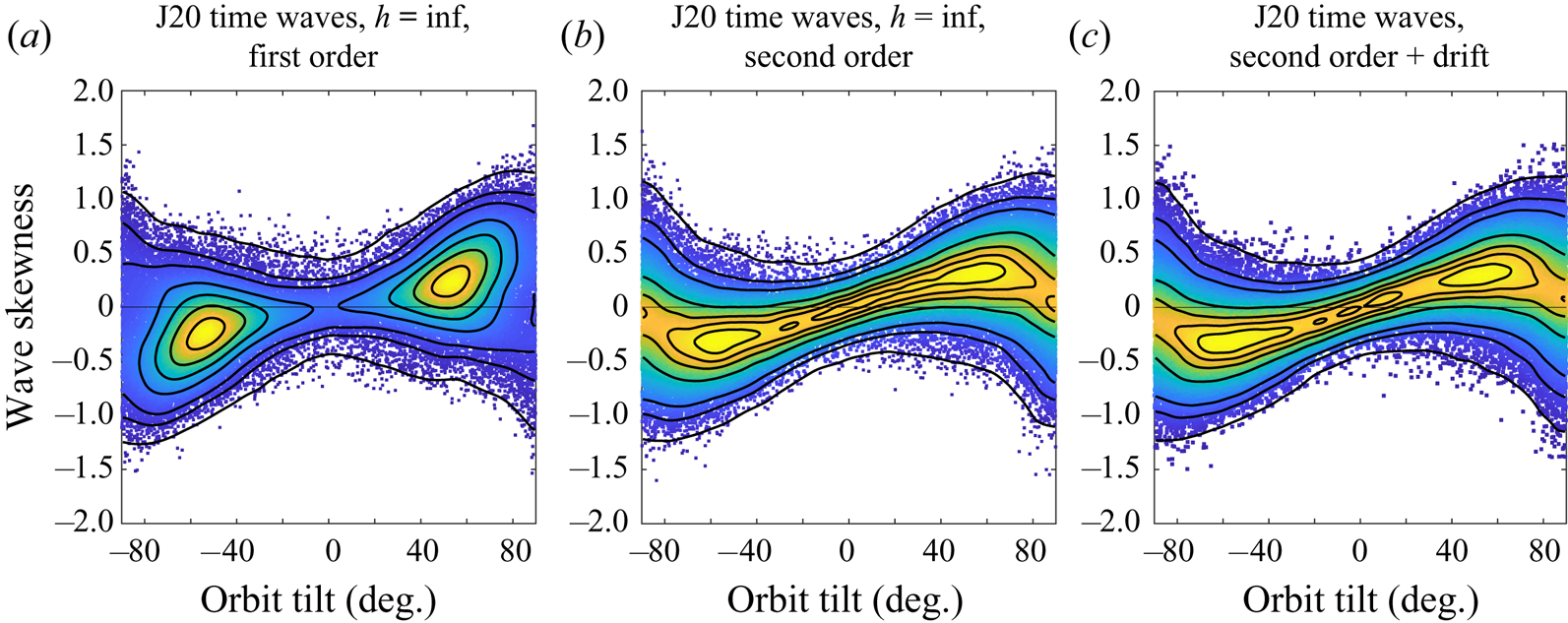
Figure 15. Tilt/skewness relation in J20 swell in time of first and second order without and with  $\text {Stokes drift} = 0.055\ \textrm {m}\ \textrm {s}^{-1}$ at infinite depth, $\textrm {BFI} = 0.87$. Each p.d.f. is based on approximately 65 000 waves.
5. Summary and conclusions
In a simulation study we have illustrated and discussed the statistical relation between the front–back asymmetry of irregular ocean waves in the Gauss–Lagrange wave model. We used two different orbital spectra, one Pierson–Moskowitz (PM) spectrum for wind driven sea states and one narrow-band JONSWAP (J20) for a strong steep swell situation. Both spectra have  $H_s = 4.5\ \textrm {m}$ and peak period $T_p = 10\ \textrm {s}$. Their Benjamin–Feir values on infinite depth are 0.23 and 0.87, respectively.
We simulated the vertical and horizontal Gaussian components of the Lagrange model and generated observable wave trains in time and in space in which we identified individual waves by the local min–max–min definition. The log ratio between the slopes before and after the local maxima was used to give a measure of wave skewness, front–back for space waves and ‘before–after’ for time waves. Only major waves with sufficient maximum height and amplitude were considered.
For each wave we identified the water particle located at the maximum at the time/location of observation and reconstructed its orbit as a function of time between the preceding and following local minima. To cope with the great variability in the shape of the orbits a standardized procedure was adopted to give a measure of orbit orientation. We did choose a least-squares fit of an ellipse to the orbits and used the inclination of its main axis as a measure of orbit tilt. This measure is sensitive to the geometry of the waves and it also reflects the increasing orbit eccentricity with decreasing depth.
The covariation between the degree of asymmetry of individual waves, as measured by the front–back skewness, and the estimated tilt of the associated particle orbits have been summarized in their bivariate p.d.f., based on between 24 000 and 150 000 pairs of waves/orbits.
The purpose of this paper has been to introduce a statistical technique to find intrinsic patterns in irregular ocean waves and test it in one common wave model, thereby complementing the model based and experimental measures mentioned in the introduction. The general conclusion of the study is that, in the Lagrange model, there is a systematic positive relation between the wave skewness and the main orientation of the orbits as estimated in the proposed method. Many factors determine the details of the joint distribution and we discuss the main findings.
5.1. The difference between time waves and space waves
Orbit tilt and wave skewness are clearly positively dependent, in both time and space, figures 1 and 2. The dependence can be seen as a summary of the wave and orbit geometry and is not coupled to the specific mathematical model that describes them. One difference between the two types of observation is how one can handle the presence or absence of Stokes drift. We have included examples of its effect on the space waves from the PM spectrum on shallow water, figure 12 and on space waves from the J20 spectrum on infinite depth in figure 14. The technique used in the study allows inclusion of a Stokes drift also in time waves, with some modification of sampling mechanism. The modification is different from that suggested in Guérin et al. (Reference Guérin, Desmars, Grilli, Ducrozet, Perignon and Ferrant2019). We have not investigated its effect on the distribution but it can be expected to be small.
5.2. Depth dependence
For both spectral types there is a typical shift in dependence with decreasing water depth, from a bi-modal p.d.f. in deep water to a unimodal p.d.f. in shallow water. Both spectra show the accompanying increase in BFI values, but further studies are needed to quantify its influence. The change is present in time waves as well as in space waves (figures 6–8) in accordance with increasing eccentricity of the orbits, cf. Wallet & Ruellan (Reference Wallet and Ruellan1950). The orientation of more eccentric ellipses will also be more exactly identified by the fitting algorithm than the more irregular orbits at great depth.
5.3. Second-order effect and the effect of Stokes drift
Inclusion of a second-order term in the model has a clear but small effect on the shape and extent of tilt/skewness dependence, as shown for PM waves in figures 12(a,b) and 13(a,b). The average Stokes drift, when added to the local model, makes a difference (figure 12c). The effect is explained in figure 10(e,f,k,l) and it is due to the elongation of orbits, that concentrates the orientation towards horizontal. For the JONSWAP spectrum the higher-order models make a bigger change, as illustrated in figures 14 and 15 except for the Stokes drift in time waves.
5.4. The dependence of the model
The observed statistical dependence is a consequence of the general wave geometry and it should be rather robust for change of spectrum. Experiments, not illustrated in the paper, with other type of spectra and characteristics confirm the general pattern for the Lagrange model. It might also be insensitive to the specific stochastic wave elevation model used, for example a second-order Eulerian model or that of Creamer et al. (Reference Creamer, Henyey, Schult and Wright1989). A systematic study of alternative models and of the random variation of the orbits around the typical shape is outside the scope of the present paper. An interesting theme for a future study would be a comparison with a similar experiment in a physical wave tank.
Declaration of interests
The authors report no conflict of interest.


 Open access