Introduction
Ice cores have become an important tool in geophysics and atmospheric chemistry. Reference Langway,Langway (1967) first perceived the great and many-sided aspects of extending physical and chemical analyses of snow and ice to what Reference Crary,Crary ([1970]) calls “the thin dimension” of glaciers, thereby adding time to the parameters considered. In a more recent paper, Reference Dansgaard,, Dansgaard,, Johnsen,, Clausen and Gundestrup,Dansgaard and others (1973) listed the potentialities of polar ice-core and bore-hole studies relevant to glaciology, meteorology, climatology, geology, volcanology, atmospheric chemistry, cosmic and solar physics, and 14C dating.
Many of the methods are applicable also on temperate glaciers (cf. Reference Árnason,Árnason (1976) for references), but melt water tends to disturb the original stratigraphy in the ice. Therefore, in some respects the polar glaciers, and in particular the dry facies of the two large ice sheets, offer the best possibilities for detailed studies far back in time.
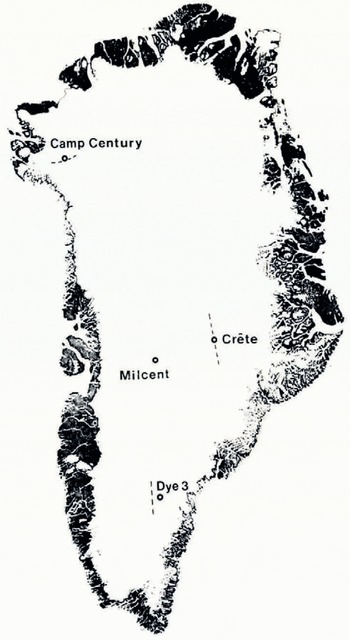
A mutual feature of all kinds of ice-core studies is the demand for a reliable time scale along the cores. The accuracy needed varies from less than 1 year (e.g. for accumulation-rate measurements) to several thousand years (e.g. for determining the sequence of glaciations). This paper is intended to review briefly the various ice-dating techniques hitherto applied and, in particular, to report on absolute, year-by-year dating by stratigraphic methods of three 400 m ice cores drilled between 1971 and 1974 under the Greenland Ice Sheet Program (GISP) (1976). At the end of the paper, Reference Dansgaard, and Johnsen,Dansgaard and Johnsen's (1969) original time scale along the Camp Century deep core back to 12 000 years B.P. will be reconsidered, on the basis of stratigraphic data. Accumulation-rate records are presented in a second paper (Reference Reeh,, Reeh,, Clausen,, Dansgaard,, Gundestrup,, Hammer, and Johnsen,Reeh and others, 1978). Station locations are shown in Figure 1.

Fig. 1. Drill sites in Greenland. CRREL drilled the first surface-to-bottom ice core at Camp Century in 1966. GISP drilled 400 m cores at Dye 3, Milcent, and Crête 1971–74. The dashed curves show the approximate course of ice divides close to three of the stations, according to data by Reference Benson,Benson (1962), Reference Mock,Mock (1963) and P. Gudmandsen (private communication).
The dating techniques applicable on ice cores or bore holes are based on (i) radioactive decay, (ii) glacier dynamical considerations, or (iii) stratigraphy. They are listed in Table I along with estimated maximum time range and accuracy, which strongly depend on the glaciological conditions at and up-stream from the drill site. Some of the short+ remarks in the fourth column are elaborated below. Exemplified references are given in the outer right column.
Table I. Ice Dating Methods

1. Radioactive Decay
Radioactive isotopes have been used for ice dating purposes since P. F. Scholander 20 years ago used the carbon-dioxide content in air bubbles for 14C dating (Reference Coachman,, Coachman,, Hemmingsen,, Scholander,, Enns, and de VriesCoachman and others, 1958). This method was further developed and applied on air released from ice melted in bore-holes by Reference Oeschger,, Oeschger, and Stauffer,Oeschger and others (1976). The time range is 500-25 000 years using 5 tons of ice. Beyond 10 000 years the 14C scale is not cali brated, which introduces an extra uncertainty onI4C dating of ice from the latest glaciation. Such calibration might be obtained by 14C dating of old ice that can be absolutely dated by other means, e.g. stable isotopes or micro-particles, see Sections 3.2.3 and 3.2.4.
No radioactive technique has been developed for dating of ice older than 25 000 years. Quite recently, Reference Muller,Muller (1977) has suggested using a cyclotron for radioisotope dating, whereby the range of the 14C method might be extended to 40 000 or 100 000 years using 1 to 100 mg carbon. Other long-lived isotopes are available: 53Mn, 36Cl, 81Kr, 26Al and 10Be (GISP, 1976) but it may be unfeasible to collect extremely small amounts of impurities from the necessary more than 100 tons of ice in a deep bore hole that has to be filled with liquid in order to prevent hole closure.
In the 100-1000 year time range 32Si and 39Ar, both with half lives close to 300 years, have been applied (Reference Clausen,Clausen, 1973; Reference Oeschger,, Oeschger, and Stauffer,Oeschger and others, 1976), but the accuracy cannot cope with that of most of the stratigraphic methods, when applicable.
Ice younger than 100 years can be dated by 210Pb. If deposited before the first thermonuclear bomb test in 1953, tritium may also be applied. But again, some of the stratigraphic methods are more accurate.
2. Glacier Dynamics
Purely theoretical, first-approximation time scales can be obtained for glaciers in steady state (thickness H and net-accumulation rate λH independent of time) by considering simple ice-flow models. If the vertical strain-rate is constant throughout the ice sheet or at least to very close to the bottom (Reference Nye,Nye, 1957), and if melting from the bottom can be neglected, the annual-layer thickness λ decreases proportional to the distanceyfrom the bottom at any location, for which H and λH do not vary up-stream. Furthermore, the horizontal velocity profile is independent of y, and with all distances expressed in metres of ice equivalent

(Reference Haefeli,Haefeli, 1961) is a usable first-approximation time scale.
If melting from the bottom cannot be neglected, λ decreases linearily with y, and reaches a value λ0 at y= o, equal to the annual ablation from the bottom. The vertical movement in the glacier thus corresponds to that in a slightly (ΔH) thicker glacier with no melting from the bottom. Equation (1) can therefore be used, if H and y are replaced by H+ ΔH and y+ΔH, ΔH being equal to Hλ0/ (λ H —λ0).
Example 1. Using the modified Equation (1) on the temperate Vatnajökull in Iceland by inserting H= 600 m, λ H = 2 m, λ0= 0.02 m (corresponding to a heat flux four times the normal 1.7 × 10⁶J m-2a-1), hence ΔH =6.1 m, gives an age of 1400 years at the bottom. This may describe the conditions in part of Vatnajökull, but of course the heat flux varies strongly from one location to another in a volcanic area.
Being purely kinematic, the above-mentioned models do not take any ice flow law into account. Nevertheless, the time scales are often fairly good approximations to absolute chronology down to considerable depths (H/2 or even 2H/3), also in cases of bottom temperatures lower than the pressure-melting point and, therefore, horizontal velocity vx = 0 at y= 0. However, in the deep part of the ice sheet, where the vertical strain-rate and therefore vx vary most with y, Equation (1) must deviate considerably from absolute chronology. In order to account for the changing strain-rates in the deep strata, Reference Dansgaard, and Johnsen,Dansgaard and Johnsen (1969) assumed

This leads to the annual layer thickness

and the consequent time scale

τ being 1 year, still with the assumption of no change of H and λ H up-stream, which of course strictly holds true only on the summit and, essentially, close to ice divides. At other locations, up-stream changes must be corrected for by using the formulae in connection with two- or three-dimensional flow models, cf. Example 5, p. 13.
Equations (3) and (4) contain three constants: H,λ H , and h, of which H and λ H are assumed to be known. At a location where the vertical temperature profile is known, the third constant,h, may be estimated by integrating Glen's or another ice flow law. Another way of estimating h is to measure the total surface strain-rate, d λ/τ dy, which is determined by Equation (3) as λ H / τ(H—h/2).
Reference Philberth, and Federer,Philberth and Federer (1971) assumed a linear temperature profile throughout the glacier and integrated Glen's law analytically. This may be an improvement in areas so far from the ice divide that the longitudinal stresses no longer affect the shape of the vx profile. It is questionable, however, if at great depths one can expect the procedure to give an approximation to absolute chronology better than that of Equation (4) , because the progressive orientation of the c-axis in favour of easy glide is difficult to account for, and in both cases an important source of uncertainty is the lack of knowledge about H, λ H , the shape of the ice sheet and temperature profiles far back in time, see Example 11, p, 20.
Example 2. Available surface data Reference Mock,(Mock, 1968) suggest that Camp Century (lat. 77° 11' N., long. 61° 09' W.) is located close to a local ice divide on the Thule Peninsula (cf. Fig. 1). Equation (4) was used withH= 1367 m,h= 400 m, λ H = 0.35 m as a first-approximation time scale along the Camp Century deep ice core by Reference Dansgaard, and Johnsen,Dansgaard and Johnsen (1969). According to this time scale,t= 10 000 years corresponds to a depth of 1120 m (y= 247 m). The validity of Equation (4) down to this depth was supported by the fact that unmistakable signs of the termination of the last glaciation were found very close to y= 247 m, i.e. a shift in δ(18O), Footnote * corresponding to a drastic increase of the surface temperature. The Camp Century time scale for the last 12000 years will be discussed in further detail in Example 11, p. 20. At this point it should only be pointed out that the apparent validity of Equation (4) does not necessarily imply that the presumptions (such as that H and λ H are independent of time) hold true. The complicated flow pattern on the Thule peninsula and its unknown changes at the end of the glaciation make it quite unlikely that any simple flow model will be able to describe a realistic time scale along the Camp Century deep core beyond t= 10 000 years, and indeed, it must be more or less a coincidence that Equation (4) gives the same time (c. 70 000 years) for the onset of the glaciation (revealed by another drastic shift in the δ profile) as other independent studies, if only for the reason that H and λ H can hardly have remained equal to their present values throughout the glaciation.
Theoretical two-dimensional flow models for steady-state ice sheets can be established to calculate the vertical strain and the resulting relationship between time and depth at a location far from the ice divide. Such flow models take into account the known changes of H, λ H and the bottom topography up-slope, and an integration of a suitable flow law based on temperature profiles consistent with the calculated flow pattern. In Example 5, p. 13, this kind of model is used and verified at Milcent, midway between the ice divide and the ice margin in mid-Greenland, but only over the upper 400 m of the total 2340 m thickness, corresponding to the last 796 years of accumulation.
Other time scales implying dynamic considerations may be established by measuring the vertical or the horizontal velocity components along a bore hole:
Close to the summit of an ice sheet in steady state, the vertical ice velocity νy is equal to the annual layer thickness at any depth. Hence, measuring a vertical velocity profile along a bore hole leads to a time scale

y being the distance from the bottom, cf. Reference Paterson,Paterson’s (1976) dating of part of an ice core through the Devon Island ice sheet. If λ H and/or H vary up-stream from the bore hole, the method is not applicable.
In the case when the horizontal velocity component νx is measured along a vertical bore hole from surface to bedrock in an area of uniform divergent flow, one may express νx as
x being the distance from the ice divide. The equation implies that H and λ H do not vary up-stream, which is of course strictly true at the summit only. In a two-dimensional flow of incompressible ice
hence

which gives the time scale when inserted in Equation (5).
3. Stratigraphy
Any kind of detectable stratification due to either unusual but well-dated events in the environments, or to regularly varying fall-out or physical conditions during deposition, can be used for the purpose of absolute dating.
3.1. Reference Horizons
Reference horizons are to be found in the form of unusual melt features (e.g. the summer of 1954 was extremely warm in North Greenland) or, more important, as unusual concentrations of impurities or heavy isotopes. The most important impurities are due to fall-out of volcanic and radioactive bomb debris.
3.1.1. Fall-Out of Fission Products.
The first thermo-nuclear bomb tests in 1952 and 1953 created a reference layer in glaciers, recognizable in Greenland by a shift in specific total β-activity in late 1953 (Reference Picciotto, and Wilgain,Picciotto and Wilgain, 1963) to approximately twice the natural level. Another more pronounced reference horizon is due to the Castle bomb-test in early 1954, performed at lat. 11° N. In Greenland the total specific β-activity increased in the period from mid-1954 to early 1955 from natural level to 5–10 times this level. In Antarctica the shift occurs in the 1954/55 summer layer to 4–5 times the natural level, which in Greenland and Antarctica is c. 100 disintegrations h-1kg-1. The bomb moratorium in 1959 caused a decrease in the fall-out towards a minimum now detectable in the 1960 layer, which is therefore a third reference horizon (not clearly detectable in Antarctica). A fourth one is to be found as extremely high activities in the 1963 layer (1964–65 in Antarctica), mainly due to the Soviet bomb tests in 1961 and 1962. The radioactive reference horizons at Milcent, mid-Greenland, are demonstrated in the first column of Figure 4 , facing p. 12. They have proved to be particularly useful for dating of firn in areas where other stratigraphic methods fail due to, for example, mixing by drift of snow from different sources (e.g. parts of the Ross Ice Shelf, receiving drift snow from the Transantarctic Mountains, Reference Clausen, and Dansgaard,Clausen and Dansgaard, 1977).

Fig. 4. Continuous δ (18O) profile along the 393 m long GISP ice core from Milcent. Dating (cf. A.D. numbers to the left of the curves) is accomplished by counting summer peaks downward from surface, the interpretation in the upper Strata being supported by the specific β-activity profile shown to the outer left. The δ values are plotted along a linear depth scale (normal figures) corrected for varying density, varying accumulation rate and ice thickness up-slope, and for total vertical strain as calculated by two-dimensional ice-flow modelling. The sloping figures are true depths in metres.
3.1.2. Volcanic Ash and Dust.
In areas close to active volcanoes, the glaciers are stratified by visible ash or dust bands in layers deposited in years of eruption. In Antarctica, dust bands (Reference Gow,Gow, 1968) may be used to establish relative chronologies between different ice cores, and in Iceland, where records of the volcanic activity span nearly a thousand years, the ash bands have been used for absolute dating of glacier ice (cf. Reference Árnason,Árnason, 1976).
3.1.3. Soluble Volcanic Debris.
In Greenland, all great northern-hemisphere volcanic eruptions, at least prior to A.D. 1766, have marked the layers deposited shortly after the eruptions with elevated specific electrical conductivity (Reference Hammer,Hammer, in press) mainly due to high concentrations of H2SO4, the sulphate originating from H2S and SO2 released from the volcano and oxidized in the atmosphere prior to wash-out.
Example 3. Figure 2 shows to the right a revised version of Reference Hammer,Hammer's (unpublished) specific-conductivity profile 1972–1765 from Station Crête (lat 71° 07' N., long. 37° 19' W.) measured on a continuous sequence of melt-water samples (one per annual layer according to absolute dating of the core, see Example 6, p. 15). The mean value (170 MΩ-1m-1) for the volcanically quiet period 1917–63 has been chosen as a base line. A dust production index (d.p.i.) is shown in the mid-section for comparison. It is based on Reference Lamb,Lamb's (1970) d.p.i., but corrected for the latitude of the eruption to account for the fact that any release of soluble impurities into the atmosphere is subject to dilution prior to deposition in Greenland, and the more the further south the eruption. As to the Icelandic volcanoes, the dominating wind pattern during eruptions may highly influence the fall-out in Greenland, cf. Hekla, 1845, or Askja, 1875, with Laki, 1783. Anyhow, the Laki eruption in 1783 also left a layer of extremely high specific conductivity in north and south Greenland. The 1783 layer may therefore be useful as a reference horizon, particularly in low accumulation areas (λ H < 0.2 m ice a-1), where the δ method fails (see p. 14).

Fig. 2. Right section: Specific conductivity profile at Station Crête spanning the period A.D. 1972–1765. Annual mean values exceeding 170 MΩ-1m-1 are set out in black. Middle section : Reference Lamb,Lamb's (1970) dust-production index corrected for latitudinal fall-out gradient. High-conductivity deposits from the Laki 1783 eruption may be used as a reference horizon in high-latitude glaciers. Left section : Micro-particle concentration profile with no significant correlation with volcanic or industrial activity. showing that the bulk of the fall-out of micro-particles in Greenland is probably due to continental dust.
3.1.4. Radio Reflection Layer.
Beyond the range of historical records of volcanic activity, radio-echo sounding has revealed internal reflection layers in the ice (Reference Gudmandsen,Gudmandsen, 1976), maybe due to high conductivity in layers from periods of high volcanic activity. The internal reflection layers are undoubtedly isochrones (Reference Robin,, Robin,, Evans and Bailey,Robin and others, 1969; Reference Whillans,Whillans, 1976) and can be traced over hundreds of kilometres. Once a series of internal reflection layers are calibrated in terms of absolute time, large parts, if not all, of the ice sheet can be dated by radio-echo sounding.
Similarly, characteristic features in the concentration of isotopes and impurities can be used to transfer a time scale from one ice core to another.
3.2. Seasonally Varying Parameters
Seasonally varying parameters reveal the annual layering of snow and ice, when measured along a line perpendicular to the layers. If the analyses are performed so as to give a continuous profile downward from the surface in sufficient detail to allow interpretation, counting of annual layers leads to an absolute time scale along the core. The necessary degree of detail to be studied depends of course on the thickness of the annual layers and on the regularity of the cycles, the criterion being that no new significant feature appears in the profile when the ice core is studied in further detail.
Extending an absolute time scale far backwards in time calls for many thousands of measurements. If this is not feasible, a (less accurate) time scale may be established by measuring the mean annual layer thickness in core increments with approximately constant age intervals giving λ as a function of y. The age in years at depth d=H—y is then

all distances being expressed in metres of ice equivalent.
3.2.1. Classical Methods
based on the detection of seasonal variations in density, crystal texture, melt features, visible dust, etc., have been reviewed elsewhere, e.g. by Reference Lamb,Langway (1967) and Reference Østrem, and Stanley,Østrem and Stanley (1969). They have only been applied beyond 200 years in a few cases (e.g. by Reference Giovinetto, and Schwerdtfeger,Giovinetto and Schwerdtfeger, 1966; Reference Gow,Gow, 1968; Reference Orheim,Orheim, 1972).
3.2.2. Radioactive Isotopes
produced in the stratosphere by cosmic radiation or by nuclear bomb tests arc mainly injected into the troposphere through the gaps in the tropopause. These gaps open up temporarily every spring, which causes increased exchange of air across the tropopause, and soon after a snow layer of high specific radioactivity is deposited on the glaciers.
Seasonal variations of the tritium content in pre-bomb layers have been demonstrated in Greenland firn (Reference Ambach, and Dansgaard,Ambach and Dansgaard, 1970; Reference Theodorsson,Theodorsson, 1977). The layers deposited after 1952 are marked by seasonally varying total specific β-activity due to fall-out of bomb debris, but in the 1963 and 1964 layers the β-activity varies irregularly. In the layers formed prior to 1965, most of the β-activity is due to90Sr and 137Cs. Some of the seasonal variations are seen in the first column of Figure 4 as small undulations superimposed on the long-term trend of the (β-activity profile. Other annual β cycles are undetectable in this profile, because the core was cut in too long samples, mainly for the purposes of detecting β reference horizons (p. 9).
3.2.3. Micro-Particles
with radii in the 0.35 to 2 μm range may be counted on melted samples by the standard Coulter technique. In this work, however, the concentrations are measured by a light-scattering technique (Reference Hammer,Hammer, 1977[a]) comprising particles down to some 0.1 μm radius. But approximately 80% of the integrated amplifier output originates from particles in the size range of the Coulter counter, 1 mV corresponding to 10000–15000 particles per gramme, somewhat depending on the size distribution.
In Greenland, the fall-out of insoluble micro-particles in the above-mentioned size range is not correlated with volcanic activity, nor has industrial activity in the last century significantly increased the atmospheric dust load in general, cf. the micro-particle concentration profile to the left in Figure 2. This shows that the bulk of micro-particles in the Greenland ice is neither of volcanic nor industrial origin. The fall-out of micro-particles varies seasonally (Reference Hamilton, and Langway,Hamilton and Langway, 1968; Reference Hammer,Hammer, 1977[a]), like the fall-out of β activity. The maximum usually occurs some time between January and July, but not always simultaneously with the β-peak, which suggests that, unlike the β-activity, the bulk of the micro-particles has been transported to Greenland via the troposphere (Reference Hammer,Hammer, 1977[b]). Most likely they consist of continental dust carried by strong winds in the upper troposphere from continental areas. According to H. Flohn (personal communication) a possible explanation for the cyclic deposition is that a blocking anti-cyclonic system occurs very regularly each spring over Greenland, causing strong, persistent winds from dry areas in North America.
Detailed micro-particle concentration profiles from Greenland will be shown in the following pages. The regular annual cycles are an excellent means for dating by counting peaks downwards from the surface, or for checking the validity of annual-layer interpretations of δ profiles that have been more or less smoothed by diffusion, cf. Figures 6 and 9. Since the micro-particles do not move by diffusion, the range of this dating method is usually longer than that based on annual δ cycles, at least back to the termination of the Wisconsin glaciation, may be much longer. But the high micro-particle concentrations in ice from the glaciation suggest very high storminess and/or atmospheric turbidity at that time, and so far no final proof has been presented that the fall-out of micro-particles varied seasonally under glacial conditions. If it did, it might call for an explanation different from that suggested by Flohn.

Fig. 6. Middle section : δ (18O) profile representing the period A.D. 1765–1805 at Crête. Ambiguities (e.g. A.D. 1784, 1789 and 1802) in the interpretation of annual layers have been solved by cross-checks with the micro-particle profile to the left that generally contains one peak of fall-out per year, and with the deconvoluted δ (18O) profile to the right that is first-order corrected for diffusive smoothing in the firn.

Fig. 9. Heavy curves: Measured δ(18O) profiles along three Camp Century ice core increments of ages ranging from 3000 to 7200 years. Thin curves: Deconvolution of the measured δ-profile by Reference Johnsen,Johnsen’s (1977) diffusion model. Section B: Counting three re-established δcycles (cf. the arrows) as annual layers is supported by peaks in the micro-particle concentration profile shown shaded to the left. Section C: The heavy arrows indicate summer melt features.
Example 4. Figure 3 shows (shaded) micro-particle concentration profiles along two increments of the Camp Century deep ice core from 1213 and 1214 m below the 1966 surface, or y= 175 m and 174 m, respectively, above the bottom. The two increments are approximately 14000 years old, according to the time scale discussed later (Example 11, p. 20).

Fig. 3. Two micro-particle concentration profiles along increments of the Camp Century ice core, both from approximately 1213 m depth corresponding to some 14000 years of age. The suggested interpretation in terms of seasonal variations (arrows at “spring” peaks) corresponds to mean annual layer thicknesses below 10 mm. The photograph shows that the micro-particle peak concentrations occur in visible cloudy bands in ice from the Wisconsin.
The former increment (Fig. 3A) was cut into 0.5 mm samples (c.400 mm2). This degree of detail was apparently more than sufficient at 1213 m depth, to judge from the smooth shape of the peaks. The background as well as the peak values are an order of magnitude higher than in post-glacial deposits. Interpretation of the profile in terms of seasonal variations suggests at most 14 and at least 10 annual layers, corresponding to a mean annual layer thickness of 5.8–8.0 mm, which is to be compared with λ = 11.2 mm calculated from Equation (3). The difference should not be considered as an indication of lower λ H under glacial conditions, because the strain history of the Wisconsin ice deep in the Camp Century core is more complicated than implied in the steady-state model behind Equation (3). As indicated by the photograph to the left in Figure 3B , the thin layers of micro-particle peak concentrations in Wisconsin ice often appear as cloudy bands detectable by eye, in particular when δ is lower than —38%, i.e. when the ice has been deposited under extremely cold conditions. The width of the cloudy bands indicates that they are not due to cracks. Again, the observed mean λ (9.2 mm) being lower than the 11.2 mm calculated from Equation (3) does not suggest lower λ H during the glaciation. But the difference between the measured λs in the two increments is one out of several indications of a positive correlation between λ and δ under extremely cold conditions, the mean δ values in the two increments being -42 and -39%, respectively.
The λ values suggested by Figure 3 are more than an order of magnitude lower than those claimed by Reference Thompson,Thompson (1977) for late Wisconsin ice in the Camp Century ice core. The discrepancy is due to the fact that the latter author used an individual sample length of no less than 17 mm, i.e. of the same order as the expected λ in the depth range considered here, which of course gives insufficient resolution.
3.2.4. Heavy Isotope and Trace Elements.
δ for the heavy isotopes 18O and deuterium in falling snow, and the concentration of some trace elements (Na, Mg, Ca, K) vary with the season (Reference Epstein, and Sharp,Epstein and Sharp, 1959; Reference Benson,Benson, 1962; Reference Dansgaard,Dansgaard, 1964; Reference Langway,, Langway,, Klouda,, Herron, and Cragin,Langway and others, 1977). The main reason for the seasonal δ variations is that, on its travel to the polar regions, a precipitating air mass is generally cooled more in winter than in summer. The δs of precipitation falling at a given location therefore generally reach lower values in winter than in summer, cf. the footnote on p. 8. But the individual snowfalls vary considerably in isotopic composition. This is why a δ profile through the uppermost layers exhibits strong variations with frequencies higher than 1 a-1, often to a degree that complicates the interpretation in terms of annual cycles. But mass exchange by diffusion via the vapour phase in the porous snow usually obliterates the high δ frequencies within a few years, depending on the temperature and the thickness of the individual layers. In areas of high accumulation and in particular those of little or no melting, the dominating 1 year δ cycle is then left in the ice as a convenient basis for absolute dating. This appears from the following considerations:
When the firnification has reached the stage where mass transport by diffusion via the vapour phase is no longer important (density c. 550 kg/m3), the amplitude of a δ cycle in a layer of thickness λ is reduced from its initial value AH to
L0 being the total mean diffusion length of the water molecules in firn, which is approximately 80 mm, essentially independent of temperature and accumulation rate (Reference Johnsen,Johnsen, 1977). According to Equation (7) the amplitudes of δ cycles in annual layers of 0.6, 0.3 and 0.2 m ice thickness is reduced by 30, 75 and 96%, respectively, at the time same as the amplitudes of high-frequency δ cycles due to individual snowfalls become undetectable: Even if we assume as few as five equally heavy snowfalls per year, the high frequency δ amplitudes are reduced by factors of 6 × 10³, 2 × 10¹⁵and 2 × 1034, respectively.
Example 5. Figure 4 shows a continuous δ record measured on an ice core 398 m long from Milcent (lat. 70° 18’ N., long. 44° 35’ W.; present mean λ H = 0.532 m ice a-1) drilled in 1973 by GISP. The core was generally cut in a sequence of eight samples per annual layer according to a preliminary time scale calculated by the steady-state two-dimensional flow model, outlined on p. 8. The flow model was verified by the fact that the preliminary time scale along the core essentially agreed with the time scale established by counting annual δ cycles downward from the surface. The upper 22 m of the firn was cut into 16 samples per calculated year, in order to study the rapid obliteration of the high frequency δ cycles. Obviously, they complicate the annual-layer interpretation in this part of the δ profile, which was therefore dated with a view to the reference horizons and, in some cases, the spring peaks in the specific total β-activity profile shown to the outer left, cf. p. 9 and 11. But below 13 m true depth the annual δ cycles stand out clearly. In agreement with Equation (6) , their mean amplitude is only reduced by some 30% during the entire firnification, and they have therefore been used for dating of the rest of the ice core by counting summer peaks downward. The bottom layer of the core was deposited 796 years prior to the year of drilling, i.e. in A.D. 1177. The δ values are corrected for decreasing δs up-slope at the sites of formation of the individual layers.
A true depth scale is shown by sloping figures in metres to the right of each column. The normal figures on the same scales are depths in metres of ice equivalent below the 1973 surface, corrected for (i) varying density; (ii) varying H and λ H up-stream; and (iii) vertical strain since the time of formation, as calculated by the two-dimensional flow model outlined on p. 8. In the corrected depth scale the layer thickness, i.e. the distance between two adjacent δ minima, therefore represents the accumulation in the corresponding time intervals (averaging one year) at the present geographic position of Milcent (Reference Reeh,, Reeh,, Clausen,, Dansgaard,, Gundestrup,, Hammer, and Johnsen,Reeh and others, 1978).
Turning back to the diffusion in the firn, it was calculated above that in layers of 0.2 m ice thickness ( = 2.5L 0), the δ amplitude is reduced by 96%, i.e. by a factor of 25. Since the amplitude of the annual δ cycles is initially of the order of 4‰, it ends up at 0.16‰, which is only twice the measuring accuracy, and hence at the limit of detection. Consequently, in areas with annual accumulation less than 0.2 m ice per year, normal annual δ cycles do not survive the firnification. This is the case in most of Antarctica, where dating by annual δ cycles can therefore generally be extended only a few decades backwards in time (Reference Johnsen,, Johnsen,, Dansgaard,, Clausen, and Langway,Johnsen and others, 1972; Reference Dansgaard,, Dansgaard,, Barkov, and Splettstoesser,Dansgaard and others, 1977). It might be more beneficial to look for seasonal variations in trace-element or micro-particle concentrations in such areas.
On most of the Greenland ice sheet, however, the annual accumulation rate is considerably higher than 0.2 m ice a-1, and the δ method therefore works thousands of years backwards in time, the only limitation being obliteration of the annual δ cycles by diffusion of the water molecule in the solid ice, see p. 18.
At stations with mean accumulation rates only slightly higher than 0.2 m ice a-1, δ cycles in years with accumulation lower than normal may be obliterated or turn into a “shoulder” on a neighbouring δ peak. If such δ records are to be applied for dating, they need to be corrected for the diffusion effect, particularly if no δ record from more favourable locations, or records of other seasonally varying parameters, are available for cross-checking. But the random character of the layer thicknesses often helps by carrying single short-periodic δ cycles through the smoothing process in a way that makes them easier to detect than one might expect from Equation (7).
This is demonstrated by the calculation experiments in Figure 5 that simulate the cutting and the analysis of the Crête core (cf. Example 6). The mean λ H is close to 0.28 m, and the core was cut into 12 samples per calculated annual layer, i.e. the sample length was 23 mm ice in layers that had not yet been exposed to significant vertical strain. The thin curves in Figure 5 are supposed to be series of “undiffused” harmonic δ cycles in annual layers, all with an amplitude of 4%. The heavy curves show how the measured δ profiles would look after firn diffusion withL0 = 0.08 m, and after addition of 0.08% noise to account for measuring uncertainty. In Figure 5A the amplitude of a series of δ cycles in layers of a subnormal 0.2 m thickness is reduced to 0.16%, i.e. twice the uncertainty and therefore at the limit of detection. In Figure 5B a series of normal 0.28 m layers is interrupted by one 0.20 m layer. In the resulting profile the thin layer appears as an easily detectable shoulder. In Figure 5C a 0.14 m layer occurs among the normal 0.28 m layers. It shows up as a deformation of the adjacent peak in the resulting profile. Finally in Figure 5D two 0.14 m layers have been introduced, causing further deformation of the adjacent peak.

Fig. 5. Calculation experiment on the diffusive smoothing of harmonic δ oscillations.
Conversely, interpretation of the measured profile in Figure 5D raises the question of how many δ cycles the nearly linear part of the curve represents. There must have been more than one—otherwise the amplitude would not have been reduced below the detection limit. But whether there were originally two or more can only be detected by a micro-particle profile and/or a deconvolution calculation that corrects for the diffusion (Reference Johnsen,Johnsen, 1977), cf. top of Figure 9B. The application of the latter technique requires an extremely well-measured δ profile, and yet the original shape of the annual δ cycles cannot be re-established in full detail, because their high-frequency components are completely obliterated.
Example 6. At Station Crête (present mean λ H = 0.282 m ice a-1) on the ice divide in central Greenland a 404 m long core was drilled by GISP in 1974. A δ profile has been measured in a continuous sequence of 12 samples per calculated annual layer along the entire core. The record comprises more than 17000 measurements and reaches back to A.D. 548. A smoothed version of it has previously been presented and interpreted in terms of climatic temperature changes (Reference Dansgaard,, Dansgaard,, Johnsen,, Reeh,, Gundestrup,, Clausen, and Hammer,Dansgaard and others, 1975). Part of the record representing the period A.D. 1765–1805, is shown in full detail in the mid-section of Figure 6 , plotted on a depth scale (corrected for vertical strain, -1.23 × 10⁻⁴a-1 (Reference Reeh,, Reeh,, Clausen,, Dansgaard,, Gundestrup,, Hammer, and Johnsen,Reeh and others, 1978)) in metres of ice equivalent below the 1974 surface. During firnification the diffusion has reduced the annual δ amplitudes considerably more than in the case of Milcent, the average λ H being only 42% higher than the critical 0.2 m ice a-1. In years of accumulation lower than 70% of normal, the original δ oscillations must therefore be nearly obliterated. The deconvoluted δ curve (L0 = 0.08 m) to the right of the measured one shows that the layers marked as 1773, 1778, 1784, 1789, 1802 and 1803 should be counted as full annual layers. Further evidence for this is to be found in the seasonally varying micro-particle concentration profile shown to the left in Figure 6 , cf. p. 16. Back to A.D. 1177 ambiguities in the Crête δ curve have been solved by cross-checks with the more regularly varying Milcent δ curve, using occasional similarities between the general shapes of the two records (cf. for example the period 1765–75 in Figure 7) ; and over the entire span of the Crête curve a few cases of doubt have been solved by cross-checking with a micro-particle profile. The reliability of this procedure was later confirmed by the close correlation between the volcanic dust production index and the specific conductivity shown in Figure 2. We estimate that the deviation of the Crête time scale from absolute chronology does not exceed two years at any time back to A.D. 1177 (three years back 10 A.D. 548).

Fig. 7. A–C: Detailed δ (18O) profiles representing the period A.D. 1765–1805 at Dye 3, Milcent and Crête. D: δ (18O) profile along a 1000±3 years older increment of the Crête ice core. The depth scales are as explained in the text to Figure 4.
Another 41 year long sequence of the Crête δ record is shown to the right in Figure 7. These layers were deposited 1000±3 years before those discussed above, i.e. in the periodA.D. 765–805. This period was generally warmer than A.D. 1765–1805, to judge from the higher mean δ value (-34.2‰ compared with -33.8‰) and assuming unchanged altitude. In fact, it was warmer than any other 40 year period since A.D. 548, cf. Reference Dansgaard,, Dansgaard,, Johnsen,, Reeh,, Gundestrup,, Clausen, and Hammer,Dansgaard and others (1975). The 765–805 δ sequence has essentially the same variance as the 1765–1805 sequence, which means that the diffusion in the firn has smoothed the original δ cycles to nearly the same extent, i.e. that the mean λ H was almost the same in the two periods. And true enough, the total thickness of the 41 old layers is only 4.7% higher than that of the 41 younger ones read on the corrected depth scale, in agreement with the linear trend at Crête (-4±2% Per millennium), cf. Reference Reeh,, Reeh,, Clausen,, Dansgaard,, Gundestrup,, Hammer, and Johnsen,Reeh and others (1978).
In case of summer melting, the shape of the δ profile after firnification depends on the degree of melting and on how the melt water percolates into the snow-pack prior to refreezing. In some cases this complicates the interpretation.
Example 7. At Dye 3 in South Greenland (lat. 65° 11' N., long. 43° 49' W.; present mean λ H = 0.54 m ice a-1) a 401 m long ice core was drilled by GISP in 1971. It was cut into 8 samples per calculated year. Part of the δ profile is shown to the left in Figure 7. Although the accumulation rate is very close to that of Milcent, the δ cycles are less regular due to refrozen melt water. The entire core length comprises 728 annual layers, of which some 15% are difficult to interpret from the δ profile. Some of the dubious layers were interpreted by micro-particle concentration analysis, cf. Figure 6 , and the rest of the interpretation problems were solved by comparing characteristic features (layer thicknesses or short-term trends in δ) with the Milcent and Crête records, cf. the period 1798–1805. The high-conductivity reference horizon left by the Laki eruption 1783 was found in the layer previously dated at 1783 as described (p. 10). Beyond age t= 190 years, the time scale is estimated to be accurate within 1% of t–190 years.
If the annual δ cycles survive the firnification process to the point where mass exchange by diffusion in air becomes negligible, they remain in the ice for thousands of years, because from that point the reduction of the δ amplitudes proceeds only by molecular diffusion in solid ice. This process is so slow (diffusion constant D= 10-8m2a-1 at -25°C) that it becomes important only when vertical strain has considerably increased the vertical δ gradients and, at the same time, reduced the annual layer thickness. If the thinning factor is θ(t) = λ(t)/ λ H , the total mean diffusion length L can be expressed by

and the δ amplitude by a generalization of Equation (7) :
AH being the δ amplitude of the annual cycle at the time of deposition (Reference Johnsen,Johnsen, 1977).
Example 8. The only existing ice core on which the theory can be checked is the Camp Century deep ice core. Using the Equations (3) and (4) for λ and age, the diffusion constant for the water molecule in ice as given by Reference Ramseier,Ramseier (1967), and the temperature profile along the Camp Century bore hole (Reference Hansen, and Langway,Hansen and Langway, 1966), Equation (8) givesL as a function of the age of the strata as shown by the heavy curve in Figure 8 ,L 0 (due to diffusion in the firn) being 80 mm. It might be easier to understand the rather complex character of the L(t) curve, if its two components, i.e. firn and solid-ice diffusion, are considered separately: If the diffusion completely ceased with the firnification, the 80 mm mean displacement of the molecules reached in the firn would simply decrease as does an 80 mm thick ice layer as it sinks toward the bottom (curve L f), i.e. in accordance with Equation (3). On the other hand, if diffusion took place only in the solid ice (i.e. L 0= 0), the mean displacement of the molecules after tyears should in principle be calculated as (2Dt)½(i.e. the mean displacement in undeformed ice), but with due account for temperature changes and vertical strain, as shown by curveL i. Equation (8) expresses the combined effect of firn and solid-ice diffusion, as shown by the heavy curveL. The full, thin curve gives the annual layer thickness λ according to Equation (3) with the present λ H . After 8700 years L(t) equals 40% of λ, and according to Equation (9) the δ amplitude in a series of years of normal accumulation has been reduced from the original 4‰ to 0.2‰, which is only three times the measuring accuracy and therefore at the limit of detection. This was essentially verified by previous measurements on the Camp Century deep ice core (Reference Johnsen,, Johnsen,, Dansgaard,, Clausen, and Langway,Johnsen and others, 1972).

Fig. 8. Total mean diffusion length L (in cm of ice equivalent) of water molecules in the Camp Century ice core, calculated by Reference Johnsen,Johnsen’s (1977) combined “reversed-diffusion” and ice-flow model, and plotted as a function of time since deposition (calculated from Equation (4)). Of the dashed curves, Lfshows L if diffusion took place in only the firn, and Lishows L in case of solid ice diffusion only. λ is the annual layer thickness calculated from Equation (3). See the text in Example 8 for further details.
As in the case of firn diffusion, δ cycles in annual layers thinner than normal disappear in the solid ice long before those in layers of normal or above-normal thickness. Nevertheless, a detailed δ profile contains information about δ cycles in thin layers, even after they have been visually obliterated. This information can be revealed by a combined “reversed diffusion” (or deconvolution) and ice-flow model (Reference Johnsen,Johnsen, 1977), which includes the model of firn diffusion that was used to reveal δ cycles “lost” during firnification at Crête.
Example 9. Figure 9 shows three measured Camp Century δ profiles (heavy curves) that have all been used as inputs to the combined deconvolution and ice-flow model in order to check for possible “lost” annual δ cycles. The outputs (thin curves) re-establish the approximate, original shape of the δ profiles, as it would have been without diffusion in firn and ice. The A-section of the figure is from an approximately 3000 year-old increment from 657 m above the bottom. According to Figure 8 ,L is 32 mm. Each of the two thickest summer layers apparently contained a double δ peak at the time of deposition (cf. Fig. 4). But no full annual δ cycles seems to have been obliterated in this increment through the last 3000 years. However, by deconvolution of δ profiles in increments older than 6000 years, new δ cycles appear. The interpretation of such cycles as annual is verified by the micro-particle profile to the left in Figure 9B , and in Figure 9C distinct melt features (indicated by arrows) support the interpretation of at least one of the re-established δ-peaks as a summer maximum.
Identification of annual layers by re-established δ cycles may be extended much further back in time at Camp Century, but generally t= 10000 years should be considered the limit of the deconvolution technique at Camp Century, because (i) the flow model used for calculating L breaks down in the Wisconsin glaciation, and (ii) λ H may have been considerably lower than at present, at least in some periods, which means much faster and more efficient obliteration of annual δ cycles, maybe even during the firnification.
Example 10. A Camp Century core increment from 217 m above the bottom, corresponding to approximately 11500 years of age, was chosen in order to check the capability of the deconvolution technique at the limit of its estimated range. The mean δ value of the increment is -36.37‰, i.e. considerably higher than normal for Wisconsin ice in the Camp Century core, which suggests that it was formed in a warm period just prior to the termination of the glaciation (Allerød, if the above-mentioned dating is correct). Deconvolution with L= 12 mm (cf. Fig. 8) reveals 11 δ peaks over 210 mm (i.e. a few more peaks than estimated by Johnsen (in press), using too high a value of L), corresponding to λ = 21 mm. However, a measured micro-particle profile contains at least 11, and at most 13 peaks over 190 mm corresponding to λ = 15.8–19.0 mm. If the micro-particle profile reveals annual layers, a few of the δ cycles may be completely obliterated. A λ value of 18 mm is twice the λ value found by Reference Hammer,Hammer (in press[a]) in an increment 1000 years younger. If the two increments were deposited in approximately the same area, it must be concluded that the accumulation rate in the warm Allerød period was much higher than in the cold Younger Dryas that followed, because a possible subsequent drastic thinning of the north-west Greenland ice sheet would have reduced the layer thickness in the two increments by nearly the same factor.
Example 11. The Camp Century time scale. In this example, we shall discuss the Camp Century time scale back to late Wisconsin on the basis of some of the methods previously described in this paper. The physical condition of the upper 950 m of the Camp Century ice core does not allow an absolute dating by measuring a continuous δ-profile along the core. In fact, it is difficult (particularly between 275 and 675 m depth) to find a sufficient number of adjoining core increments long enough to allow determination of representative λ-values. In general, many such values, closely spaced in time, are needed for using Equation (6) , p. 11, to establish a time scale. However, analyses of the GISP ice-core records suggest that in post-glacial time relatively few, well-determined mean λ-values may be sufficient in Greenland, due to surprisingly stable accumulation conditions. For example, at Crête, λ H has had a secular trend of only -4±2% through 1000 years, cf. Reference Reeh,, Reeh,, Clausen,, Dansgaard,, Gundestrup,, Hammer, and Johnsen,Reeh and others (1978). Furthermore, the short-term and the areal variabilities are small enough to ensure a reasonable accuracy of mean values of λ determined on a few annual layers, Footnote *
In Figure 10 we have compiled new micro-particle and isotope data, as well as previously published isotope data, in some cases adjusted by the deconvolution technique. The measured and (belowy= 180 m) the estimated λ-values are plotted against y, in Figure 10 over the entire core above y= 100 m, and in Figure 11 on extended scales below y= 450 m. The small figures at the points indicate the number of identified annual layers.

Fig. 10. Annual layer thickness, λ (scale on top), in the Camp Century ice core plotted against depth and distance y above the bottom. The heavy curve is the least-squares fit of Equation (3) to all data with y >250 m. The corresponding time scale derived from Equations (3) and (4) is plotted along the sloping axis. The dashed curve is the least-squares fit, when using Reference Philberth, and Federer,Philberth and Federer’s (1971) procedure. The figures close to the points are the number of annual layers interpreted in the individual core increments, either directly from δ (18O) profiles (open squares), or after deconvolution (open circles), or from measured micro-particle profiles (filled circles), or just by visual stratigraphy (filled squares, cf. the photograph in Figure 3).

Fig. 11. Details of the data and curves in Figure 10 for y <420 m. The shaded curve is the δ(18O) profile for 20 < y < 368 m plotted in 4 m intervals. δ values below -31% reveal the Wisconsin glaciation. The time scale to the outer right is based on the heavy curve (Equation (4)). It is estimated to be accurate within ±3% back to 10000 B.P. If correction is made for the significantly deviating λ values in the y interval 220 to 240 m, the age of the late glacial δ peak indicated by an arrow becomes 11400±400 B.P.
If λu and λl are the upper and lower limits of λ estimated by interpreting a sufficiently detailed profile in terms of annual layers, we use (λu+ λl)/2 as a representative for λ, and (λu- λl)/2 for σi. As for σa, the long λ H records from Dye 3, Milcent and Crête, and short records from the vicinity of these stations, show that the relative total variability of λ H , (σa/λ H ), is only 20–35%, essentially independent of time and locality. Moreover, in the high-frequency range (>0.05 a-1) the λ H records are closely modelled by a Gaussian process. Hence, the statistical error of ann(<20) year mean value may be written σ a= σa/✓n= 0.22 λ/✓n, and the total uncertainty of a mean value determined by interpretation of annual cycles is
According to Section 2 above, there are at least two possibilities for comparing the observed λs with theoretical or semi-empirical, steady-state flow-model calculations:
-
I. The curve drawn in full in Figures 10 and 11 is derived from Equation (3) with λ H = 0.382 m and h= 429 m, which gives a least-squares fit to all data withy250 m. The fit is perfect, in so far as σλ(i.e. the r.m.s. of the deviations of the measured λ-values weighted with 1/σλ 2) is 5.1 × 10⁻³m, equal to the r.m.s. of the λ-values themselves (5.2 × 10⁻³m). The consequent time scale, calculated by Equation (4) is plotted on the sloping axis. The age t= 10000 years is reached at y= 236 m. To the right in Figure 11 the Camp Century δ profile is plotted in 4 m increments over the y-interval 20 to 368 m. The Wisconsin glaciation is revealed by the low δs from y= 40 to y= 248 m. The above-mentioned time scale dates the late glacial δ peak, indicated by an arrow, at 10900 years B.P. If the low λ-values in the 220–240 m y-interval are accounted for, the age of the δ peak becomes 11350 years, which agrees with 14C dating of the Allerød interstadial (11800 to 11000 B.P. (Reference Tauber, and Olsson,Tauber, 1970).
The uncertainty σtI of age t in the zero to 10000 year interval has been calculated with due account for the co-variance between the λ H and h uncertainties, cf. for example Reference Whittaker, and Robinson,Whittaker and Robinson (1924, p. 242). σtI varies from 2.2% for very small ages to 1.4% for t= 5500 years. At t= 10000 years, σtI = 1.7%.
-
II. Another time scale may be derived by Reference Philberth, and Federer,Philberth and Federer’s (1971) procedure outlined on p. 000. The νx -profile implied is similar to that of Reference Weertman,Weertman (1968) and may be adequately approximated by
withp= 5.9,vxH -value at the surface. The optimum fit of the corresponding λ profile to our λ data is obtained for λ H = 0.353 m a-1, but σ λ is significantly higher (9.5 × 10⁻³m) than that obtained by using Equation (3) , cf. the thin, dashed curve in Figure 10.(10)
One might speculate whether the reason for the relatively poor fit of Philberth and Federer’s model is that Camp Century is lying so close to a local ice divide that the flow in the deep ice is determined by longitudinal stresses rather than shear stresses. This would invalidate Philberth and Federer’s integration of Glen’s law and imply a lower shear strain in the deep ice.
-
III. The best fit of a λ-profile of the type given by Equation (10) is obtained for p= 3.74 and λ H = 0.396 m a-1, which gives σ λ= 6.3×10⁻³m, i.e. not significantly different from σ λ in case I. The consequent time scales are therefore not significantly different. σ tIII varies from 3.1% for very small ages to 1.8% for t= 6000 years. At t= 10000 years, σ tIII= 2.1%. The relative deviation Δt/t from the time scale defined by Equation (4) as stated under I above, does not exceed 2.5% for anytup to 10000 years.

We conclude that the time scale (Equation (4)), shown in Figures 10 and 11 is a satisfactory approximation to absolute chronology for the last 10000 years at Camp Century, in so far as it is fully consistent with all available λ data. This supports the steady-state assumption behind Equations (3) and (4) , or in other words that the present flow pattern on the Thule peninsula was established prior to 10000 B.P. Beyond 11500 B.P., the available λ-data do not allow any correction of the time scale given by Equation (4).
3.3. Long-term δ Oscillations
In an attempt to correct the time scale for changing Hλ H through the glaciation, Reference Dansgaard,, Dansgaard,, Johnsen,, Clausen, Langway, and Turekian,Dansgaard and others (1971) used the hypothesis that the long-term Camp Century δ profile contains oscillations with constant periods due to regularly varying solar radiation. Regular variations with periods of 415 and 2500 years are found in the rate of production of 14C Reference Suess, and Olsson,(Suess, 1970), and seem to be in antiphase with the δ profile for t< 10000 years. Apparently persistent, long-term δ oscillations, not strictly periodic in the time scale given by Equation (4) , were given a constant period of 2400 years for t10000 years, and for t< 10000 years a shorter-term δ oscillation was given a constant period of 415 years. Reference Fisher,Fisher (unpublished) and Reference Paterson,, Paterson,, Koerner,, Fisher,, Johnsen,, Clausen,, Dansgaard,, Bucher and Oeschger.Paterson and others (1977) have later shown that using the 2400 years cycle over the entire core length brings the resulting time scale in closer agreement with stratigraphic observations and to Equation (4) in the 0 to 10000 years interval. The validity of the resulting time scale at great depths still remains to be verified.
Acknowledgements
The authors are indebted to many people for their co-operative efforts that have been the foundation of this work throughout several years. Our thanks are due to our colleagues within the U.S.–Swiss–Danish Greenland Ice Sheet Program, in particular Lyle Hansen, Chester C. Langway, Steve Mock and John Rand, of U.S. Army, Corps of Engineers, Cold Regions Research and Engineering Laboratory; to Hans Oeschger, Henry Rufli and Bernhard Stauffer, of the University of Bern; who all participated in the GISP drilling and sampling activities; to Preben Gudmandsen and his staff at Technical University of Denmark, who carried out the radio-echo sounding programme, and to Karl Kuivinen and John Clough, PICO, University of Nebraska—Lincoln, for their excellent field-operation management. Within our own laboratory we owe sincere thanks to the technicians Ellen Emme, Anita Boas and Tove Stougaard, and to the instrument makers Steffen Hansen and Jan Nielsen, who also participated in the field work. Earnie Mains, ITT, Hugo Thomsen, DAG, and Sten Malmquist, KGH, were of great help to us in Søndre Strømfjord, Greenland.
Finally, we want to express our appreciation to U.S. National Science Foundation, Division of Polar Programs (head Dr Robert H. Rutford), for continuous interest and logistic support, executed by Alaskan Air Command, U.S. Air Force, and by VXE-6 Squadron U.S. Navy; and to the Ministry of Greenland and the Danish Natural Science Research Council for funding the Danish contribution to GISP.