


1. Introduction
Self-aeration is a fascinating flow phenomenon that is frequently observed in high-Froude-number open-channel flows (figure 1). Such flows are characterised by strong turbulence and neither surface tension nor gravity are able to maintain surface cohesion (Brocchini & Peregrine Reference Brocchini and Peregrine2022), causing entrainment of air bubbles into the flow column. These bubbles subsequently break down into a wide range of bubble sizes (Lamarre & Melville Reference Lamarre and Melville1991; Deane & Stokes Reference Deane and Stokes2002; Deike, Melville & Popinet Reference Deike, Melville and Popinet2016; Chan, Johnson & Moin Reference Chan, Johnson and Moin2021), and eventually penetrate towards the channel bottom through turbulent diffusion. It is known that entrained air can significantly alter flow properties, thereby leading to flow bulking, drag reduction, cavitation protection and enhanced gas transfer (Straub & Anderson Reference Straub and Anderson1958; Falvey Reference Falvey1990; Gulliver, Thene & Rindels Reference Gulliver, Thene and Rindels1990; Kramer et al. Reference Kramer, Felder, Hohermuth and Valero2021).

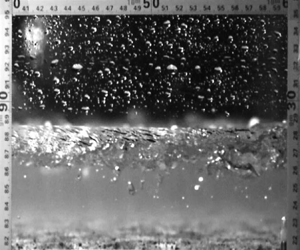
Figure 1. Self-aeration in high-Froude-number flows: (a) the TWL of a flow over a microrough channel bed at the Water Research Laboratory, UNSW Sydney, Australia; specific water flow rate  $q = 0.188$ m $^2$ s $^{-1}$; chute angle $\theta = 10.8^\circ$; streamwise distance from invert $x = 6.3$ to $6.5$ m; image courtesy of Armaghan Severi, adapted with permission; (b) schematic of the TWL of a self-aerated flow down a smooth chute, including a differentiation between entrapped, entrained and total conveyed air.
As such, the characterisation and the modelling of air concentration distributions has been subject to sustained research interest over the last decades. Different groups of researchers have conceptualised the air concentration using single-layer (Rao & Gangadharaiah Reference Rao and Gangadharaiah1971; Wood Reference Wood1991; Chanson & Toombes Reference Chanson and Toombes2001; Valero & Bung Reference Valero and Bung2016; Zhang & Chanson Reference Zhang and Chanson2017) or double-layer approaches (Straub & Anderson Reference Straub and Anderson1958; Killen Reference Killen1968; Wei & Deng Reference Wei and Deng2022; Wei et al. Reference Wei, Xu, Deng and Guo2022). Based on visual observations, various physical processes have been identified in self-aerated flows, comprising generation of free-surface waves, surface disruption, air entrainment, turbulent diffusion of air bubbles and ejection of droplets. It is argued that single-layer approaches are unable to represent these different flow processes, while good data-driven agreement between single-layer models and measurements has been achieved, which is, however, at the expense of empirically fitted coefficients. Recently, Kramer & Valero (Reference Kramer and Valero2023) presented a physically based two-state convolution formulation for the air concentration that is built upon a turbulent boundary layer (TBL) and a turbulent wavy layer (TWL).
It is important to note that none of the previous single-layer or double-layer air concentration conceptualisations have taken into account the contribution of entrapped and entrained air, as depicted in figure 1(b), which is introduced in the following. In a seminal series of experiments, Killen (Reference Killen1968) investigated surface characteristics of self-aerated flows by deploying a common phase-detection probe as well as a larger-sized conduction probe that dipped in and out of the surface roughness/waves, hereafter referred to as a dipping probe. Wilhelms & Gulliver (Reference Wilhelms and Gulliver2005) reanalysed the data of Killen (Reference Killen1968) and pointed out that the dipping probe measured entrapped air, transported between wave crests and troughs, whereas the common phase-detection probe measured a combination of entrapped and entrained air, termed total conveyed air. Although Wilhelms & Gulliver (Reference Wilhelms and Gulliver2005) articulated the need for two measurements, one for entrapped air and one for total conveyed air, no other researchers have deployed a dipping probe since, showing the uniqueness of Killen's (Reference Killen1968) data set.
The key novelty of the present work is the introduction of a superposition principle, which explicitly accounts for entrapped air (waves) and entrained air (bubbles), allowing us to quantify the importance of different physical mechanisms to the mean air concentration. In the following, the two-state formulation of Kramer & Valero (Reference Kramer and Valero2023) is briefly summarised (§ 2.1). Thereafter, the superposition principle for the air concentration of the TWL is proposed, demonstrating that entrapped air and entrained air follow a Gaussian error function and a normal distribution, respectively (§ 2.2). The superposition principle is then combined with the two-state convolution in § 2.3, providing the most complete and physically consistent description of the air concentration distribution to date. A bed-normal integration of this expanded formulation allows us to differentiate between three different physical mechanisms that contribute to the mean air concentration, comprising entrapped air within the TWL, entrained air within the TWL and entrained air within the TBL (§ 2.3). The different parameters of the superposition principle as well as the application of the new formulation are assessed against Killen's (Reference Killen1968) data set in § 3, followed by a discussion on model applicability and other limitations (§ 4).
2. Methods
2.1. Two-state convolution
This section provides a brief summary of the governing equations of the two-state convolution model, while more details are presented in Kramer & Valero (Reference Kramer and Valero2023). The air concentration of the TBL ( $\bar {c}_{TBL}$) is reflected through a solution of the advection–diffusion equation for air in water, whereas the air concentration of the TWL ( $\bar {c}_{TWL}$), encompassing bubbles and waves, was found to follow a Gaussian error function (Kramer & Valero Reference Kramer and Valero2023)
 \begin{gather} \bar{c}_{TBL} =\begin{cases} {\bar{c}_{\delta/2}} \left({\dfrac{y}{\delta-y}} \right)^{\beta}, & y \leq \delta/2, \\ \bar{c}_{\delta/2} \exp \left(\dfrac{4\beta}{\delta} \left(y - \dfrac{\delta}{2} \right) \right)\!, & y > \delta/2, \end{cases} \end{gather}
 \begin{gather} \bar{c}_{TWL} = \frac{1}{2} \left( 1 + \operatorname{erf} \left( \frac{y - y_{50}}{ \sqrt{2} \mathcal{H} } \right) \right)\!, \end{gather}
where  $\bar {c}_{\delta /2}$ is the air concentration at half the boundary layer thickness ( $\delta$), $y$ is the bed-normal coordinate, $\beta = \bar {v}_r S_c /\kappa u_*$ is the Rouse number, $\bar {v}_r$ is the bed-normal bubble rise velocity, $\kappa$ is the van Kármán constant, $u_*$ is the friction velocity and $S_c$ is the turbulent Schmidt number, defined as the ratio of eddy viscosity and turbulent mass diffusivity. Further, $\mathcal {H}$ is a characteristic length scale that is proportional to the thickness of the TWL, $\operatorname {erf}$ is the Gaussian error function and $y_{50}$ is the mixture flow depth where the total conveyed air concentration is $\bar {c} = 0.5$; note that other mixture flow depths are represented in the same manner, e.g. $y_{90} = y(\bar {c}=0.9)$. The two-state model assumes a fluctuating interface that separates the TBL and the TWL, and a convolution of the two states with a Gaussian interface probability leads to the following expression for the mean air concentration (Krug, Philip & Marusic Reference Krug, Philip and Marusic2017; Kramer & Valero Reference Kramer and Valero2023)
 \begin{equation} \bar{c} = \bar{c}_{TBL}(1-\varGamma) + \bar{c}_{TWL} \varGamma, \end{equation}
with
 \begin{equation} \varGamma(y; y_\star, \sigma_\star) = \frac{1}{2} \left( 1+\operatorname{erf} \left(\frac{y - y_\star }{ \sqrt{2} \sigma_\star} \right) \right)\!, \end{equation}
where  $y_\star$ is the time-averaged interface position and $\sigma _\star$ is its standard deviation. It is noted that the two-state formulation (2.3) has been successfully validated against more than 500 air concentration data sets from the literature, hinting at universal applicability. For more information on the development of (2.1) to (2.4), as well as on the definition and determination of associated physical model parameters, the reader is referred to Kramer & Valero (Reference Kramer and Valero2023).
2.2. Superposition principle (TWL)
Herein, it is hypothesised that the air concentration of the TWL results from a superposition of waves and entrained air bubbles, which was similarly proposed by Wilhelms & Gulliver (Reference Wilhelms and Gulliver2005) for the mean air concentration. To formulate this principle, the focus is set on a flow situation where aeration is confined to the wavy layer, similar to figure 1. The entrapped air concentration of the TWL can be interpreted as the probability of encountering entrapped air at a certain location within the flow. In a time-averaged sense, this probability can be expressed as  $p(\bar {c}_{trap}) = \mathcal {V}_{trap}/\mathcal {V}_{tot}$, where $\mathcal {V}_{trap} =$ volume of entrapped air and $\mathcal {V}_{tot} = \mathcal {V}_{trap} + \mathcal {V}_{ent} + \mathcal {V}_{W} =$ total volume of the mixture, including the volume of entrained air ( $\mathcal {V}_{ent}$) and the volume of water ( $\mathcal {V}_{W}$). The probability of encountering an entrained air bubble within a wave is $p(\bar {c}^*_{ent} \mid \bar {c}_{trap}) = \mathcal {V}_{ent}/(\mathcal {V}_{ent} + \mathcal {V}_{W})$, which is a conditional probability, given that a wave/water phase is present. Considering the two complementary events $\bar {c}_{trap}$ and $(1 - \bar {c}_{trap})$, the expression for the total conveyed air concentration of the TWL reads
 \begin{equation} \bar{c}_{TWL} = \bar{c}_{trap} + (1 -\bar{c}_{trap})\bar{c}^*_{ent}. \end{equation}
It is recognised that
 \begin{equation} (1 -\bar{c}_{trap}) \bar{c}^*_{ent} = \frac{\mathcal{V}_{ent} + \mathcal{V}_{W}}{\mathcal{V}_{tot}} \frac{\mathcal{V}_{ent}}{\mathcal{V}_{ent} + \mathcal{V}_{W}} = \frac{\mathcal{V}_{ent}}{\mathcal{V}_{tot}} = \bar{c}_{ent}, \end{equation}
where  $\bar {c}_{ent}$ is the entrained air concentration, defined as the volume of entrained air bubbles related to the total mixture volume. Combining (2.5) and (2.6) leads to the final superposition equation for the TWL (figure 2)
 \begin{equation} \bar{c}_{TWL} = \bar{c}_{trap} + \bar{c}_{ent}. \end{equation}
Figure 2. Representation of Killen's (Reference Killen1968) measurements in a self-aerated flow with  $q = 0.78$ m $^2$ s $^{-1}$, $\theta = 30^\circ$ and $x = 7.4$ m; (meas, measured): (a) total conveyed air concentration, measured with a common phase-detection probe; (b) entrapped air concentration, measured with a dipping probe; (c) entrained air concentration, determined through the superposition principle.
It is noted that the total conveyed air concentration  $\bar {c}_{TWL}$ is described by (2.2), c.f. figure 2(a). Valero & Bung (Reference Valero and Bung2016) discussed that the entrapped air concentration $\bar {c}_{trap}$ follows an analytical solution of the air–water surface height distribution, which is (also) reflected by a Gaussian error function (see figure 2b)
 \begin{equation} \bar{c}_{trap}= \frac{1}{2} \left(1 + \operatorname{erf} \left(\frac{y - y_{50_{trap}}}{\sqrt{2} \mathcal{H}_{trap}} \right) \right)\!, \end{equation}
where  $y_{50_{trap}}$ corresponds to the mean water level, and $\mathcal {H}_{trap}$ is the root-mean-square wave height. Rearranging (2.7), an analytical solution for the entrained air concentration can be written as
 \begin{equation} \bar{c}_{ent} = \bar{c}_{TWL} - \bar{c}_{trap} =\frac{1}{2} \left(\operatorname{erf} \left( \frac{y - y_{50}}{\sqrt{2} \mathcal{H}} \right) - \operatorname{erf} \left( \frac{y - y_{50_{trap}}}{ \sqrt{2} \mathcal{H}_{trap} } \right) \right)\!. \end{equation}
 Figure 2(c) shows that the entrained air concentration corresponds to the difference of two cumulative Gaussians (2.9), which in turn reflects a Gaussian distribution. Further parameters of interest are the peak entrained air concentration  $\bar {c}_{max}$ and its corresponding position $y_{\bar {c}_{max}}$, which were added to figure 2(c) for completeness. It is emphasised that these two parameters are not necessarily required, as the profile of entrained air (TWL) is mathematically defined by (2.9).
2.3. Combining both approaches
In § 2.2, the superposition principle was formulated for flow situations where aeration is confined to the wavy layer (pure TWL, compare figures 1 and 2). In practice, air bubbles are often diffused deeper into the flow column, one example being shown in figure 3, where it is seen that the superposition principle still holds for the TWL (figure 3a). In order to explicitly account for the contribution of entrapped and entrained air within the TWL, the two-state convolution (2.3) is combined with the superposition principle (2.7)
 \begin{equation} \bar{c} = \left(\bar{c}_{trap} + \bar{c}_{ent}\right) \varGamma + \bar{c}_{TBL}(1-\varGamma), \end{equation}
which describes the complete air concentration profile, see figure 3(b). Further, (2.10) can be integrated between the channel invert and  $y_{90}$, yielding an expression for the depth-averaged (mean) air concentration
 \begin{align} \langle \bar{c} \rangle &= \frac{1}{y_{90}} \int_{y=0}^{y_{90}} \bar{c} \, \text{d}y \end{align}
 \begin{align} &= \underbrace{\frac{1}{y_{90}} \int_{y=0}^{y_{90}} \bar{c}_{trap} \varGamma \, \text{d}y}_{\langle \bar{c} \rangle_{{TWL}_{trap}} } + \underbrace{\frac{1}{y_{90}} \int_{y=0}^{y_{90}}\bar{c}_{ent} \varGamma \, \text{d}y}_{\langle \bar{c}\rangle_{{TWL}_{ent}}} + \underbrace{\frac{1}{y_{90}}\int_{y=0}^{y_{90}} \bar{c}_{TBL}(1-\varGamma) \, \text{d}y}_{\langle \bar{c} \rangle_{TBL}}. \end{align}
Figure 3. Representation of Killen's (Reference Killen1968) measurements in a self-aerated flow with  $q = 0.39$ m $^2$ s $^{-1}$, $\theta = 52.5^\circ$, $x = 3.7$ m: (a) superposition principle; (b) two-state air concentration convolution.
Equation (2.10) represents the most complete and physically consistent description of the air concentration distribution in self-aerated flows to date. Its integrated form (2.12) allows us to differentiate between three different physical mechanisms contributing to the mean air concentration, comprising: (i) entrapment of air due to free-surface deformations; (ii) entrainment of air due to turbulent forces exceeding gravity and surface tension forces; and (iii) turbulent diffusion of air bubbles into the TBL, represented through  $\langle \bar {c} \rangle _{{TWL}_{trap}}$, $\langle \bar {c} \rangle _{{TWL}_{ent}}$ and $\langle \bar {c} \rangle _{TBL}$, respectively.
3. Results
The application of the superposition principle requires two different measurements, one for entrapped air and one for total conveyed air. Commonly, the total conveyed air has been measured using intrusive phase-detection probes, e.g. Straub & Anderson (Reference Straub and Anderson1958), Chanson & Toombes (Reference Chanson and Toombes2001), Bung (Reference Bung2009) and Severi (Reference Severi2018), whereas entrapped air has rarely been measured, one exception being the smooth chute data from Killen (Reference Killen1968, 20 profiles), to which the expanded formulation of the two-state model is applied. This reanalysis of all 20 profiles is presented in Appendix A, and more details of the original measurements are provided in table 1. Here, the local Froude-number is defined as  $Fr = q / (g d_{eq}^3)^{1/2}$, with $g$ being the gravitational acceleration and $d_{eq} = \int _{y=0}^{y_{90}} (1-\bar {c})\,\text {d}y$ the equivalent clear water flow depth.
Table 1. Experimental flow conditions of Killen (Reference Killen1968); all reanalysed profiles extracted from Wilhelms & Gulliver (Reference Wilhelms and Gulliver1994, tables B1 to B4); note that the profile number corresponds to Appendix A.
 $k_s\ is\ \text {roughness height}$; $\text {chute length} = 15.25$ m; $\text {chute width} = 0.46$ m
The two free parameters  $\mathcal {H}$ and $\mathcal {H}_{trap}$ of the superposition principle were obtained through least squares fitting. Here, $\mathcal {H}$ was obtained by minimising the sum of squared differences between measurements and modelled air concentrations within the upper flow region, while the full profile was used for determination of $\mathcal {H}_{trap}$, as depicted in figure 3(a). The flow depths $y_{50}$ and $y_{50_{trap}}$ could be directly extracted from Killen's (Reference Killen1968) data, and were therefore regarded as fixed. Other free and fixed parameters of the two-state convolution ( $\beta$, $y_\star$, $\sigma _\star$, $\bar {c}_{\delta /2}$ and $\delta$) had already been determined by Kramer & Valero (Reference Kramer and Valero2023), and are therefore not discussed hereafter. In the following, the results of the reanalysis of Killen's (Reference Killen1968) measurements are presented.
3.1. Physical parameters of the TWL
Figure 4(a) shows the length scale of the of the TWL ( $\mathcal {H}$) as well as the root-mean-square wave height ( $\mathcal {H}_{trap}$), both normalised with $y_{90}$ and plotted against the mean air concentration. Similar to the data of Kramer & Valero (Reference Kramer and Valero2023), there was a linear dependence between $\mathcal {H}$ and $\langle \bar {c} \rangle$. The present analysis reveals that the length scale of the TWL ( $\mathcal {H}$) and the root-mean-square wave height ( $\mathcal {H}_{trap}$) showed some similar trends (figure 4a), which implies that $\mathcal {H}$ can provide a rough indication for $\mathcal {H}_{trap}$, while it is acknowledged that $\mathcal {H}$ may not capture the full complexity of the air–water interface geometry. Further, the empirical three-sigma rule was applied to show that $\mathcal {H}$ corresponded to the difference between the characteristic flow depths $y_{84}$ and $y_{50}$ (figure 4b), which was also applicable to $\mathcal {H}_{trap}$ (not shown). It is worthwhile to mention that roughness effects as well as the streamwise dependence of model parameters are implicitly accounted for in $\langle \bar {c} \rangle$.

Figure 4. Physical parameters of the TWL for the data of Killen (Reference Killen1968): (a) length scale  $\mathcal {H}$ and root-mean-square wave height $\mathcal {H}_{trap}$ versus mean air concentration; (b) three-sigma rule applied to evaluate $\mathcal {H}$; (c) characteristic depths $y_{50}$ and $y_{50_{trap}}$ versus mean air concentration.
As discussed in Kramer & Valero (Reference Kramer and Valero2023), the normalised flow depth  $y_{50}$ was linearly related to the mean air concentration (figure 4c). In contrast, the mean water depth $y_{50_{trap}}$ was found to be less dependent on $\langle \bar {c} \rangle$, and $y_{50_{trap}}/y_{90}$ became constant for $\langle \bar {c} \rangle > 0.4$ (figure 4c). The difference between $y_{50}$ and $y_{50_{trap}}$ was indicative for the downwards shift of the Gaussian error function for entrapped air, compare figure 3(a).
3.2. Mean air concentration decomposition
Figure 5(a) confirms that predicted mean air concentrations (2.12) were in good agreement with measured mean air concentrations, the latter directly evaluated from phase-detection intrusive measurements using (2.11). Note that (2.12) was numerically integrated, incorporating the analytical solutions for the  $\bar {c}_{TBL}$ (2.1), $\bar {c}_{trap}$ (2.8), $\bar {c}_{ent}$ (2.9), as well as $\varGamma$ (2.4).

Figure 5. Mean air concentrations derived from Killen's (Reference Killen1968) data: (a) measured mean air concentrations versus (2.12); (b) contribution of different physical mechanisms to the mean air concentration as per (2.12).
Equation (2.12) allows us to differentiate between three different physical mechanisms contributing to the mean air concentration. It was found that  $\langle \bar {c} \rangle _{TBL}$ and $\langle \bar {c}\rangle _{{TWL}_{ent}}$ increased with increasing $\langle \bar {c} \rangle$, whereas the entrapped air concentration of the TWL was approximately constant, at $\langle \bar {c} \rangle _{{TWL}_{trap}} \approx 0.1$ (figure 5b; profiles ordered by $\langle \bar {c} \rangle$), which hints at the fact that the geometry of the (mean) air–water interface of the TWL varied only slightly in Killen's (Reference Killen1968) experiments. Note that a constant entrapped mean air concentration was previously reported by Wilhelms & Gulliver (Reference Wilhelms and Gulliver2005), which is further corroborated by recent computations of the free-surface roughness wavelength distribution in supercritical flows (Valero & Bung Reference Valero and Bung2018, figure 12). More generally, the deformation of the free-surface in shallow turbulent flows, and therefore the entrapped air concentration, is known to be driven by various processes, including the interaction of turbulent coherent structures with the water surface, resonant wave growth and effects of bed topography (Valero & Bung Reference Valero and Bung2016; Muraro et al. Reference Muraro, Dolcetti, Nichols, Tait and Horoshenkov2021; Brocchini & Peregrine Reference Brocchini and Peregrine2022). While effects of these different processes on entrapped and entrained air concentrations have not been studied in the past, the current decomposition of the mean air concentration provides a versatile framework that allows us to assess the contribution of individual physical mechanisms.
3.3. Streamwise self-aeration development and equilibrium state
In figure 5(b), the profiles of Killen's (Reference Killen1968) four measurement series (table 1) were ordered by increasing  $\langle \bar {c} \rangle$, which is appropriate to exemplify general trends of $\langle \bar {c} \rangle _{{TWL}_{trap}}$, $\langle \bar {c}\rangle _{{TWL}_{ent}}$ and $\langle \bar {c}\rangle _{TBL}$ with respect to $\langle \bar {c} \rangle$. To provide more insights on $\langle \bar {c} \rangle$ and its controlling parameters, it is important to point out different distinct regions in self-aerated flows, including the non-aerated developing flow region, the aerated gradually varied flow (GVF) region and the aerated uniform flow (UF) region (figure 1b), which have been described in the literature, e.g. Wood (Reference Wood1991) and Chanson (Reference Chanson1996), amongst others. In the GVF region (figure 1b), the mean air concentration $\langle \bar {c} \rangle$ depends on the streamwise location with respect to the inception point of air entrainment ( $L_i$, figure 1b), as well as on the slope $\theta$ and (similarly) on the Froude-number. In contrast, the mean air concentration in the UF region, termed equilibrium mean air concentration $\langle \bar {c}\rangle _\infty$ (figure 1b), is known to be solely a function of $\theta$ (or $Fr$) (Hager Reference Hager1991; Matos Reference Matos1995).
Figure 6(a) compares equilibrium air concentrations from Straub & Anderson (Reference Straub and Anderson1958) with the present reanalysis, showing that Killen's (Reference Killen1968) measurements were taken in the GVF region. Following Wei & Deng (Reference Wei and Deng2022), Killen's (Reference Killen1968) mean air concentrations are normalised with their equilibrium value, approximated as  $\langle \bar {c} \rangle _\infty = 0.75 \sin \theta ^{0.75}$ (Hager Reference Hager1991), and plotted against the dimensionless streamwise coordinate $(x-L_i)/L_i$ (figure 6b,c). This normalisation shows a good collapse of the four different measurement series, thereby demonstrating how the two-state superposition model can be used to finely differentiate between different physical processes in the streamwise decomposition of $\langle \bar {c} \rangle$. The evolution of $\langle \bar {c} \rangle _{TBL}$ displays asymptotic behaviour towards equilibrium and is well described by an analytical solution of the continuity equation for air in water (Appendix B)
 \begin{equation} \langle \bar{c} \rangle_{TBL} = \langle \bar{c} \rangle_{{TBL}\infty} \left(1 - \exp \left(-\frac{u_r \cos \theta}{q} (x - L_i) \right) \right)\!, \end{equation}
where  $\langle \bar {c} \rangle _{{TBL} \infty }$ is the equilibrium mean air concentration of the TBL, and $u_r$ is the depth-averaged bubble rise velocity. Here, (3.1) was evaluated for Killen's (Reference Killen1968) data on the $52.5^\circ$ slope, and good agreement with measurements was achieved using $u_r = 0.1$ m s $^{-1}$ and $\langle \bar {c} \rangle _{{TBL}\infty } = 0.53 \langle \bar {c} \rangle _{\infty }$ (figure 6b). The mean air concentration $\langle \bar {c} \rangle$ similarly approaches equilibrium, and an additional comparison with data from Straub & Anderson (Reference Straub and Anderson1958) reveals that the length of the GVF region is approximately four to six times $L_i$ (figure 6b). Further, figure 6(c) shows that the trends in $\langle \bar {c} \rangle _{{TWL}_{trap}}$ and $\langle \bar {c} \rangle _{{TWL}_{ent}}$ are opposite for $(x-L_i)/L_i \lessapprox 2$, which is consistent with experimental observations of free-surface roughness/waves, but no entrained air, upstream of the inception point of free-surface aeration (Felder, Severi & Kramer Reference Felder, Severi and Kramer2022). In the GVF region, around $(x-L_i)/L_i \gtrapprox 2$, the contributions of $\langle \bar {c} \rangle _{{TWL}_{trap}}$ and $\langle \bar {c} \rangle _{{TWL}_{ent}}$ become approximately constant, which suggests that equilibrium for the TWL is achieved farther upstream than for the TBL. Additional research is required to confirm these findings.

Figure 6. Equilibrium air concentration and streamwise self-aeration development: (a) equilibrium air concentrations  $\langle \bar {c} \rangle _\infty$ and $\langle \bar {c} \rangle _{{TBL} \infty }$ versus Froude-number for the data of Straub & Anderson (Reference Straub and Anderson1958), compared with non-equilibrium concentrations from Killen (Reference Killen1968); (b,c) evolution of depth-averaged (mean) air concentrations in Killen's (Reference Killen1968) high-Froude-number flows.
4. Discussion: model applicability and limitations
In § 2.2, the superposition principle (2.7) was formulated for flow situations where aeration is confined to the wavy layer of a supercritical free-surface flow, i.e. a pure TWL, and it was combined with the two-state convolution (2.10) to account for flows where the air bubble diffusion layer protrudes to the channel bottom, see § 2.3. Therefore, the bottom air concentration  $\bar {c}_0$, defined as the air concentration in the vicinity of the solid invert (Hager Reference Hager1991; Kramer et al. Reference Kramer, Felder, Hohermuth and Valero2021), is a natural choice to exemplify the application range of proposed equations. Figure 7 shows a plot of $\bar {c}_0$ versus $\langle \bar {c} \rangle$, illustrating that (2.7) is valid for $\langle \bar {c} \rangle \lessapprox 0.25$, while (2.10) is valid for $\langle \bar {c} \rangle \gtrapprox 0.25$. It is noteworthy mentioning that the total conveyed air concentration is fully described by the two-state convolution (2.3) introduced by Kramer & Valero (Reference Kramer and Valero2023), while the superposition principle provides additional physical insights into the structure of the TWL, given that additional measurements of entrapped air are made.

Figure 7. Applicability of the proposed equations for smooth chute flows: variation of  $\bar {c}_0$ versus $\langle \bar {c} \rangle$.
The model parameters of the extended two-state superposition principle (2.10) are the Rouse number ( $\beta$), the boundary layer thickness ( $\delta$), the air concentration at half the boundary layer thickness ( $\bar {c}_{\delta /2}$), the transition/interface parameters $y_\star$ and $\sigma _\star$, mixture flow depths $y_{50}$ and $y_{{50}_{trap}}$, as well as the length scale of the TWL ( $\mathcal {H}$) and the root-mean-square wave height ( $\mathcal {H}_{trap})$. Of these parameters, $y_{50}$, $y_{50_{trap}}$, $\bar {c}_{\delta /2}$ and $\delta$ were directly extracted from measurements, whereas $\beta$, $y_\star$, $\sigma _\star$, $\mathcal {H}$ and $\mathcal {H}_{trap}$ were obtained through fitting. It is acknowledged that the predictive capability for some parameters is currently limited, which is, however, deemed acceptable, as the aim of the present model is to establish a physically based description of the air concentration distribution, with physical parameters responding to the flow. Further details on $\mathcal {H}, \mathcal {H}_{trap}$, $y_{50}$ and $y_{{50}_{trap}}$ are presented in figure 4, while the interface parameters and the Rouse number range between $\beta = 0.05$ to 1.2, $y_\star /\delta = 0.6$ to 0.9 and $\sigma _\star /\delta = 0.1$ to 0.2 (Kramer & Valero Reference Kramer and Valero2023).
As mentioned before, the application of the superposition principle requires two separate measurements, one for entrapped air and one for total conveyed air. Killen (Reference Killen1968) used a common intrusive phase-detection probe for the measurement of total conveyed air, while a larger-sized dipping probe was used for the measurement of entrapped air. It is emphasised that these measurements are unique, and no other researchers have deployed a comparable set-up since. Future measurement of entrapped air, either through a measurement set-up similar to that of Killen (Reference Killen1968) or via non-intrusive measurement techniques, such as acoustic displacement meters (Cui, Felder & Kramer Reference Cui, Felder and Kramer2022) or laser time-of-flight or triangulation sensors, are of high relevance to increase our fundamental physical understanding of air–water flow processes, which is anticipated to lead to an improvement/revision of some existing modelling approaches, e.g. for air–water mass transfer in supercritical flows (Bung & Valero Reference Bung and Valero2018; Kramer Reference Kramer2020).
Lastly, it is stressed that the two-state superposition model has been developed for statistically steady self-aerated flows on steep slopes in prismatic rectangular channels. However, the model can readily be adapted to characterise air concentration distributions of other statistically steady self-aerated flows in prismatic geometries, e.g. hydraulic jumps. The application to unsteady aerated flows, such as breaking waves, is more involved and requires the hundredfold repetition of experiments, followed by an application of ensemble-averaging techniques, see Blenkinsopp & Chaplin (Reference Blenkinsopp and Chaplin2007) and Whutrich, Shi & Chanson (Reference Whutrich, Shi and Chanson2022).
5. Conclusion
In this work, a novel superposition principle for entrapped and entrained air within the TWL of a supercritical open-channel flow is presented. The corresponding air concentration distributions for entrapped air and total conveyed air both follow a Gaussian error function, while entrained air is characterised by a Gaussian normal distribution. The free parameters of the mathematical formulation are the root-mean-square wave height and the length scale of the TWL, which are shown to be of similar magnitude and dependent on the mean air concentration. Subsequently, the superposition principle is combined with the two-state convolution of Kramer & Valero (Reference Kramer and Valero2023), representing the most complete and physical description of the air concentration distribution to date. A bed-normal integration of this combined equation allows us to differentiate between three different physical mechanisms that contribute to the mean air concentration, comprising entrapment of air due to free-surface deformations, entrainment of air due to turbulent forces and turbulent diffusion of air bubbles into the TBL. The subsequent analysis of the streamwise development of these mechanisms suggests that the equilibrium for the TWL is achieved farther upstream than for the TBL. While further research is required to confirm this finding, the presented application nicely demonstrates how the two-state superposition model can be used to uncover new flow physics in self-aerated flows. It is acknowledged that only a limited data set was analysed herein, which is because the quantification of entrapped air requires specific flow measurement instrumentation, i.e. a dipping probe.
Overall, it is anticipated that the presented theory holds for a wide range of high-Froude-number self-aerated flows, encompassing the range tested by Straub & Anderson (Reference Straub and Anderson1958,  $5 \lessapprox Fr \lessapprox 32$). A meaningful extension of this work would comprise a thorough development/testing of new sensors for the non-intrusive measurement of entrapped air, as well as the development of advanced phase-detection signal processing techniques that allow us to discriminate between entrapped and entrained air. These developments are to be followed by detailed investigations on the functional dependence between model parameters and flow/geometric properties, including bottom-surface roughness, friction velocity, flow depth, as well as other statistical measures of bulk flow and turbulence. A better understanding of the underlying physics of self-aerated flows will enable the formulation and implementation of more physically consistent numerical models for air entrainment and transport.
Acknowledgements
M.K. would like to thank Dr D. Valero (Karlsruhe Institute of Technology, KIT) for fruitful discussions; Professor D. Bung (FH Aachen) for proofreading and sharing of data sets; and Dr A. Severi (Manly Hydraulics Laboratory) for sharing her images.
Funding
This research received no specific grant from any funding agency, commercial or not-for-profit sectors.
Declaration of interests
The author reports no conflict of interest.
Data availability statement
All data, models or code that support the findings of this study are available from the corresponding author upon reasonable request.
Appendix A. Reanalysis of Killen's (Reference Killen1968) measurements
This appendix presents the application of the combined superposition two-state formulation to 20 concentration profiles of Killen's (Reference Killen1968) data set, with corresponding flow conditions indicated in table 1. In figure 8, each measured profile with  $\langle \bar {c} \rangle \gtrapprox 0.25$ is represented by two subpanels. In the first subpanel, identified by i, the superposition principle is plotted with its corresponding (2.8), (2.9), (2.7), together with the profile number, chute angle ( $\theta$), specific discharge ( $q$) and streamwise distance ( $x$ in metres) from the upstream crest. Each second subpanel (identified by ii) contains plots of the two-state formulation (2.1), (2.7), (2.10), including the mean air concentration. For $\langle \bar {c} \rangle \lessapprox 0.25$, the air concentration distribution is characterised by the superposition principle alone, and only the first subpanel is plotted (index dropped). The numbering of the profiles increases with streamwise distance for each test series, as per table 1, and the background of every first profile of the four series is shaded in grey.

Figure 8. Twenty concentration profiles of Killen's (Reference Killen1968) data set, with corresponding flow conditions indicated in table 1.
Appendix B. Streamwise evolution of  $\langle \bar {c} \rangle _{TBL}$

To develop an equation for the streamwise evolution of  $\langle \bar {c} \rangle _{TBL}$, the continuity equation for entrained air within the TBL is written (Wood Reference Wood1985)
 \begin{equation} \frac{\text{d} (q_{a_{TBL}})}{\text{d}\kern0.06em x} = v_e - \langle \bar{c} \rangle_{TBL} u_r \cos \theta, \end{equation}
where  $q_{a_{TBL}}$ is the specific air flow rate of the TBL per unit width, $v_e$ is the entrainment velocity of air into the TBL, and $u_r$
$u_r$  $\cos \theta$ represents detrainment of air, with $u_r$ being a depth-averaged rise velocity of air bubbles. It is noted that previous researchers used the total air flow rate $q_a$ instead of $q_{a_{TBL}}$, which, however, is thought to be incorrect, as the volume of entrapped air, for example in the developing non-aerated region, is not balanced by rising air bubbles. Similar to Wood (Reference Wood1985), it is now assumed $q_{a_{TBL}}/q \approx \langle \bar {c} \rangle _{TBL}$; note that this assumption represents a simplification, and more elaborate relationships for $q_{a_{TBL}}/q$ may be used, see Wood (Reference Wood1991) and Chanson (Reference Chanson1996), which, however, would not lead to an explicit solution. Substitution of $q_{a_{TBL}}/q \approx \langle \bar {c} \rangle _{TBL}$ into (B1) leads to
 \begin{equation} q \frac{\text{d} \langle \bar{c} \rangle_{TBL}}{\text{d}\kern0.06em x} = v_e - \langle \bar{c} \rangle_{TBL} u_{r} \cos \theta. \end{equation}
In the UF region (figure 1), streamwise gradients vanish, implying that (B2) simplifies to
 \begin{equation} 0 = v_{e\infty} - \langle \bar{c} \rangle_{{TBL}\infty} u_{r \infty} \cos \theta, \end{equation}
where  $v_{e \infty }, \langle \bar {c} \rangle _{{TBL} \infty }$ and $u_{r \infty }$ are the entrainment velocity, mean air concentration, and bubble rise velocity in the UF region. Equation (B3) is now subtracted from (B2), further assuming $v_e \approx v_{e \infty }$ and $u_r \approx u_{r \infty }$
 \begin{equation} q \frac{\text{d} \langle \bar{c} \rangle_{TBL}}{\text{d}\kern0.06em x} = u_r \cos \theta \left(\langle \bar{c} \rangle_{{TBL}\infty} - \langle \bar{c} \rangle_{TBL} \right)\!. \end{equation}
Separating variables
 \begin{equation} \frac{1}{\langle \bar{c} \rangle_{{TBL}\infty} - \langle \bar{c} \rangle_{TBL}}\,\text{d} \langle \bar{c} \rangle_{TBL} = \frac{u_r \cos \theta}{q} \text{d}\kern0.06em x, \end{equation}
and integrating between the inception point of air entrainment ( $x = L_i$) and an arbitrary downstream location
 \begin{equation} \int_{0}^{\langle \bar{c} \rangle_{TBL}} \frac{1}{\langle \bar{c} \rangle_{{TBL}\infty} - \langle \bar{c} \rangle_{TBL}} \text{d} \langle \bar{c} \rangle_{TBL} = \frac{u_r \cos \theta}{q} \int_{x=L_i}^{x} \text{d}\kern0.06em x, \end{equation}
yields the following solution
 \begin{equation} \ln \left(\frac{\langle \bar{c} \rangle_{{TBL}\infty}} {\langle \bar{c} \rangle_{{TBL}\infty} - \langle \bar{c} \rangle_{TBL} } \right) = \frac{u_r \cos \theta}{q} \left( x - L_i \right)\!, \end{equation}
where the lower limit of the integral on the left-hand side of (B6) corresponds to the entrained air concentration at the inception point, which per definition  $\langle \bar {c} \rangle _{TBL}(x=L_i) = 0$. Equation (B7) can be rearranged/simplified to obtain the following analytical expression for the streamwise development of $\langle \bar {c} \rangle _{TBL}$
 \begin{equation} \langle \bar{c} \rangle_{TBL} = \langle \bar{c} \rangle_{{TBL}\infty} \left( 1 - \exp \left(-\frac{u_r \cos \theta}{q} (x - L_i)\right) \right)\!. \end{equation}
 This equation provides a simple method to characterise the increase of the mean air concentration of the TBL as function of the equilibrium air concentration ( $\langle \bar {c} \rangle _{{TBL}\infty }$), depth-averaged bubble rise velocity ( $u_r$), slope ( $\theta$), specific water flow rate ( $q$) and the streamwise distance from the inception point of air entrainment ( $x-L_i$). Substituting $q=\langle\bar{u}\rangle_{i}\,d_{i}$, with $\langle\bar{u}\rangle_{i}$ and $d_{i}$ being the mean water velocity and the water depth at the inception point, Wilhelms & Gulliver's (Reference Wilhelms and Gulliver2005, eq. 4) empirical relationship can be recovered
 \begin{align} \langle \bar{c}\rangle_{TBL} = \langle \bar{c} \rangle_{{TBL}\infty} \left( 1 - \exp \left(-\frac{u_r \cos \theta}{\langle\bar{u}\rangle_{i}}\frac{x-L_{i}}{d_{i}}\right) \right)=
\langle \bar{c} \rangle_{{TBL}\infty}\left(1 - \exp \left(-\alpha\frac{x - L_{i}}{d_{i}}\right) \right),\end{align}
\begin{align} \langle \bar{c}\rangle_{TBL} = \langle \bar{c} \rangle_{{TBL}\infty} \left( 1 - \exp \left(-\frac{u_r \cos \theta}{\langle\bar{u}\rangle_{i}}\frac{x-L_{i}}{d_{i}}\right) \right)=
\langle \bar{c} \rangle_{{TBL}\infty}\left(1 - \exp \left(-\alpha\frac{x - L_{i}}{d_{i}}\right) \right),\end{align}
thereby revealing that their coefficient  $\alpha=(u_{r} \cos \theta)/\langle\bar{u}\rangle_{i}$ corresponds to a dimensionless bubble rise velocity. In order to solve equations (B8) or (B9), the unknowns $u_{r}$ and $\langle\bar{c}\rangle_{{TBL}\infty}$ need to be determined. One can perform some air-water flow measurements or, alternatively, use a best-fit approach.


