Introduction

A frequently overlooked aspect of radio echosounding is the potential for gaining information on the small-scale roughness of subglacial surfaces. This small-scale roughness might typically have a vertical scale of less than 0.5 m and so be unresolvable by conventional sounders. Nonetheless it is responsible for the fading patterns normally seen on Z records and the echo tail extension on A-scope displays. If the possibility is admitted that rock types might be characterized by their small-scale roughness, or that freezing and melting regimes on an ice shelf might be so identified, the importance of trying to estimate surface roughness becomes apparent. The present paper details one such study using data from the Ross Ice Shelf gathered with the Scott Polar Research Institute/Technical University of Denmark 60 MHz radio echo sounder.

Preamble

The connection between the structure of radio echoes and small-scale roughness has been extensively studied by Reference BerryBerry (1973), Reference HarrisonHarrison (1972) and Reference NealNeal (1977). Of necessity, all three analyses start by specifying a theoretical form for the reflecting surface. Kirchoff diffraction theory is then used to make statistical deductions about the echo shape and fading pattern for a complete range of roughness characteristics. Comparison of measured and theoretical statistics may then yield the required information on small-scale roughness. The major weakness of this approach lies in the fact that a priori assumptions have to be made about the form of the surface. To counter this, the theoretical surface is chosen to be as general as is mathematically convenient. The outcome is the so-called Gaussian distributed random surface. It is random in the sense that there is no functional relation describing the surface.

Instead, vertical deviations from the mean horizontal plane are specified by a Gaussian probability distribution. Variation in the horizontal plane is governed through a prescribed auto-correlation function. This leaves two parameters to be determined from the radio echo: the vertical root mean square (RMS) displacement of the surface from its mean plane a and σ the horizontal correlation length L. Associated with σ a is a phase shift ϕ₀=4πσ/λ_s where λ_s represents the radar wavelength at the reflecting surface. This parameter describes the phase modulation imposed upon the radio echo by the surface roughness.

From a practical point of view, it is much easier to measure the spatial, along-track, fading patterns of the radio echo than to make detailed measurements of the echo shape. This is especially true since the work of Reference HarrisonHarrison (1972) and Reference NealNeal (1977) indicates that the statistics of the fading pattern may be generated, with only a small margin of error, by digitizing the peak echo power from the surface under investigation. The implication is that data may be taken from echo strength measurement (ESM), records (Reference NealNeal 1976) or a series of closely spaced A-scope frames. The present study uses A-frames since these allow simultaneous investigation of the ice/air and ice/water interfaces. It is, of course, necessary that the along track spacing of these A frames should satisfy Nyquist's sampling criterion. This states that at least two samples must be taken within the period of the highest frequency component in the fading pattern. The highest frequency component would arise from interference between two point targets at diametrically opposite sides of the radio echo footprint. This situation yields an interfering signal in which the maxima are separated by

where λ is the radar wavelength in air (5 m),p is the length of the radar pulse in air (18 m), n is the refractive index of ice (1.78), d is the terrain clearance, and I is the ice thickness. Substituting values for d and I from Table I gives a minimum spacing of 8 m. The 2 m spacing of the A-frames is, therefore, well within the necessary sampling rate.

As a preliminary to the main analysis, it is necessary to check that the fading pattern contains a usable amount of information about the reflecting surface. It will do so if the angle subtended at the antenna by the radar footprint exceeds the RMS slope of the surface roughness. According to Reference NealNeal (1977), a simple way to check this is to see whether the spacing of power maxima in the fading pattern A satisfies

(1)

From Figure 4 and Table I it can be seen that, for the ice/water interfaces under consideration here, the spacing of power maxima easily satisfy Equation (1). Surface information is therefore present in the fading pattern and further analysis is warranted.

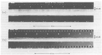
Fig.4. ESM records of the power returned from the ice/water interfaces at (a) 77^°25'S, 171^°38'E and (b) 84^°24'S, 163^°43'W.

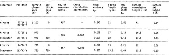
Table I STATISTICS OF THE REFLECTING SURFACES DERIVED FROM ILLUMINATION WITH A 60 NS, 60 MHz RADIO ECHO PULSE

Determination of σ from the probability distribution of the received power

As a first step in the analysis, it is instructive to examine the distribution of peak echo power. This is simply the relative frequency of different peak powers appearing in a succession of individual A-frames along the track section under investigation. Comparison of the measured and theoretical distributions will yield a value for σ, and, at the same time, will show how well the Gaussian random surface fits reality

The theoretical power distribution is derived from the distribution of complex amplitude P(A) presented in Reference Beckmann and SpizzichinoBeckman and Spizzlchino (1963). To use their expression, however, it is necessary to specify a probability distribution for the phase angle of the resultant scattered amplitude vector. A determination of this distribution is extremely difficult until the Fraunhofer region of diffraction, defined by R = λ(d+I/n)/πL² > 2 is reached. Note that this means that the aircraft must be high enough with respect to the correlation length of the surface under investigation. In the Fraunhofer region, the phase angle of the scattered amplitude becomes uniformly distributed between 0 and 2π and the amplitude distribution takes the form

(2)

in which A₀ and A_v ² represent the mean and variance of A respectively. I_om is the modified Bessel function of the first kind and zeroth order. It is worth noting that A₀ is equal to the amplitude of the unscattered component of the power spectrum. Equation (2) is commonly known as the Rice distribution. As far as interpreting the observed power distributions is concerned, it is fortunate that the radio echo transceiver is usually situated in the Fraunhofer diffraction zone.

As shown by Reference BramleyBramley (1955), the power in the unscattered component is a fraction exp(-ϕ₀ ²) of that in the incident signal, so A_o ^→0 for ϕ₀ ²>>1. This situation arises when the signal is fully modulated by a very rough surface. In this case, Equation (2) reduces to

(3)

and the received amplitude is, therefore, Rayleigh distributed

For a fairly smooth surface, ϕ₀ ²≪l and the amplitude variance is now roughly equal to the power in the scattered components which is given by A₀ ²ϕ₀ ² This limit also allows the Bessel function in Equation (2) to be replaced by its asymptopic form I_0m(x) = exp(x)/√2πx and the resulting amplitude distribution is found to be given by

(4)

The power distributions corresponding to Equations (3) and (4) are easily obtained by setting P = A². This gives

(5)

for ϕ₀ ²≫1 and

(6)

for ϕ₀ ² ≪1.P₀ represents the mean received power. For radio echo sounders using a logarithmic receiver, a more useful form of these distributions is obtained by expressing the received power in dB relative to the mean power level. In this case, Equations (5) and (6) transform into

(7)

and

(8)

respectively, where

and

The distributions represented by Equations (7) and (8) are plotted in Figure 1 for several values of ϕ₀. The width of these curves increases with ϕ₀ up to the point where the echo becomes fully modulated. It is this behaviour which enables an estimate of ϕ₀, and hence σ,to be made from a comparison of the theoretical and experimental distributions

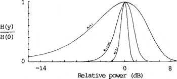
Fig.1. Theoretical distributions of the power received in the Fraunhofer diffraction region from surfaces of specified roughness. They have been normalized so that the maximum value of P(P) is unity.

Two power distributions, returned from the top surface of the ice shelf, are shown in Figure 2. Also included in this figure are returns from a crevasse field and a calm surface of the Ross Sea. Returns from these surfaces are analysed in an attempt to provide “control” surfaces through which the analysis can be checked. It should, however, be noted that a system of crevasses does not constitute a Gaussian random surface and its inclusion is primarily intended to demonstrate the realization of the Rayleigh distribution for rough surfaces

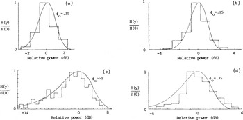
Fig.2 Normalized distributions of power returned from:(a) Ice/air interface at 77^°25'S, 171^°38'E, (b) Ice/air interface at 84^°24'S, 163^°43'W,(c) Crevassed ice/air interface at 83^°38'S, 158^°00'W, (d) Calm sea surface at 77^°14'S, 171^°54'W.

Bearing in mind the fact that the digitized power records are only accurate to 0.5 dB, it is seen that a good match can be made between the theoretical and experimental distributions. In this way, the use of a Gaussian random surface is partially justified and an estimate of ϕ₀ = 0.15 rad is obtained for the ice/air interface. The corresponding value for o is a not unreasonable 60 mm. For the crevassed surface ϕ₀>>1 and the vertical roughness scale is, therefore, much greater than 0.4 m. The RMS phase shift produced by the sea surface is estimated at 0.35 rad, which implies a vertical deviation of 140 mm.

Figure 3 shows two power distributions returned from the bottom surface of the ice shelf. The corresponding ESM records are given in Figure 4. The first distribution emanates from a smooth surface near the ice front, whilst the second indicates a comparatively rough bottom. Once again, there is a good match between the experimental and theoretical distributions, and the RMS phase shifts in the two cases are estimated at 0.125 and 0.425 rad. Attributing all of this phase shift to bottom roughness leads to derived values for a of 30 and 100 mm, respectively

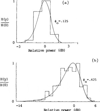
Fig.3. Normalized distributions of power returned from: (a) Ice/water interface at 77^°25'S, 171^°38'E. (b) Ice/water interface at 84^°24'S, 163^°43'W.

Determining σ and L from the power variance and fading length

The normalized power variance V_p is obtained from the digitized data by computing

(9)

in which P(x) represents the peak power in the return at position x along the traverse. The fading length τ_p is found from the auto-correlation function

(10)

It is defined as the distance over which ρ_p falls to the value of 0.37 and is directly measured from a plot of ρ_p against μ. Correlation plots for the ice/air, ice/water, and air/sea boundaries are presented in Figure 7. Table I lists the computed values of v_p and the measured values of τ_p

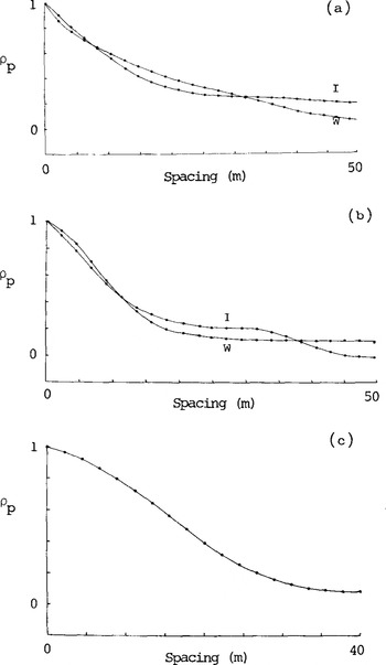
Fig.7. Auto-correlation function of power returned from(a) position 77^°25'S, 171^°38'E. I is ice/air interface, W is ice/water interface.(b) position 84^°24'S, 163^°43'W. I is ice/air interface, W is ice/water interface. (c) position 77^°14'S, 171^°54'E. Air/water interface

Figures 5 and 6 provide the basis for determining σ and L from v_p and τ_p. These curves show the dependence of the power variance and fading length on distance from the reflecting surface and have been adapted from figures 1 and 3 of Reference Bramley and YoungBramley and Young (1967). To account for the finite length of the radio echo pulse, their set of curves, derived for continuous-wave (cw) illumination, has been modified in accordance with

(11)

and

(12)

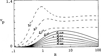
Fig.5. Normalized variance vp as a function of R, normalized height above the surface, for a surface illuminated with a 60 ns Gaussian pulse. ϕ₀ represents the RMS phase modulation imposed upon the radio echo by the surface roughness. The dashed curves correspond to cw illumination and are taken from figure 1 of Reference Bramley and YoungBramley and Young (1967).

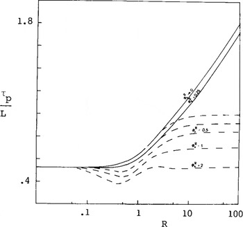
Fig.6. Horizontal scale size as measured by the ratio of fading length τ_p to the horizontal correlation length L for a surface illuminated with a 60 ns pulse. The dashed curves correspond to cw illumination and are taken from figure 3 of Reference Bramley and YoungBramley and Young (1967).

These equations are limiting cases of complex general expressions given in Reference NealNeal (1977) and are useful whenever ϕ₀ ² <0.3. Beyond this point, extensive numerical evaluation of the general expression is required, and it is, therefore, fortunate that Bramley and Young's original curves can be used without much error whenever Equation (1) is satisfied. The new parameter introduced in Equation (11) is defined by

It is interesting to note that when Equation (1) is satisfied,Г→0) and Equations (11) and (12) reduce to equations (28) and (29) of Reference Bramley and YoungBramley (1967).

Taking the experimental values for V_p and τ_p, Figures 5 and 6 are used in an iterative manner to deduce the roughness parameters given in the table. It may be seen that the values for ϕ₀ derived in this way are slightly higher than those deduced from the complete echo power distributions. This arises because the power variance in a pulsed sounder is lower than that in a cw system as indicated by Equation (11).

Effect of a non-smooth ice/air boundary on returns from the ice-shelf base

In order to deduce σ from ϕ₀, it has been assumed that the surface under investigation is totally responsible for the modulation of the radio echo. This is certainly true for returns from the ice/air boundary, but is definitely not so for basal echoes. These must pass through the non-smooth top surface and may be modulated by traversing a nonuniform layer of basal saline ice. Reference NealNeal (1977) shows that this latter phenomenon can produce sufficient modulation to prevent an assessment of physical roughness. It is, therefore, fortunate that the presence of saline ice can be detected with fair accuracy by measuring the radio frequency absorptive losses of the ice shelf (Reference NealNeal 1979). This prevents erroneous attribution of detected phase shift to small-scale roughness.

Given that it is possible to analyse data from zones clear of saline ice, the fact remains that the ice/air boundary must always be negotiated. Its influence on basal returns has therefore been investigated by computing the cross-correlation coefficient between the surface and basal fading patterns. The value of this parameter, together with the total number of samples, is recorded in Table I. Its statistical significance can be readily assessed by referring to the 't' distribution. In this way, the correlation between the ice/air interface and smooth ice-shelf bottom is found to be significant at the 10% level. In contrast, there is no significant correlation between returns from the ice/air interface and the 'rough' ice/water boundary.

Reference NealNeal (1977) gives a theoretical backing to these observations by extending the Kirchoff approach to deal with basal reflection through an ice/air interface. For cases in which the power variance is less than about 0.5 and the transceiver lies in the Fraunhofer region of the diffraction pattern, the general expression for v_p reduces to

(13)

where ϕ₀B represents the basal phase shift. ϕ₀T represents the RMS phase shift introduced into the signal in passing through the ice/air boundary. This is simply related to the rf dielectric constant of the surface snow ε and the RMS phase shift upon reflection ϕ₀R by

Values for ϕ₀R are available from Table I, whilst √ε may be deduced using the relationship between refractive index and firn density given in Reference Robin, Evans and BaileyRobin and others (1969). Snow of density 400 kg m ³ has a predicted refractive index of 1.32 and Equation (13) is therefore equivalent to

By comparing the values of ϕ₀R and ϕ₀B from Table I, it is seen that the effect of the ice/air interface on the variance of the power returned from the ice shelf base is extremely small. This explains the low significance of the cross-correlation coefficients