

Introduction
Growing global food demand, especially from the emerging markets, and fluctuating fuel prices have become important drivers of U.S. farmland values (Henderson, Gloy, and Boehlje Reference Henderson, Gloy and Boehlje2011). Studies show that expanding ethanol production may have also pushed up farmland values in the United States (e.g., Henderson and Gloy Reference Henderson and Gloy2009, Kropp and Peckham Reference Kropp and Peckham2012). Aside from the macroeconomic and policy environment, the recent upward trend in farmland markets has attracted increasing attention from investors and real estate private equity funds. Farmland provides an opportunity to invest in an asset class that is not directly correlated to stocks and derivatives markets, with relatively less volatility (Miller Reference Miller2012). These features make farmland an excellent instrument to help rebalance portfolios and offset risks in real estate investment. According to Nickerson et al. (Reference Nickerson, Morehart, Kuethe, Beckman, Ifft and Williams2012), nonoperators (landowners who do not themselves practice agriculture) own a large portion of U.S. farmland, as high as 29 percent of land in farms in 2007. Based on the most recent U.S. Census of Agriculture, the number increased to 30 percent in 2012 (Bigelow, Borchers, and Hubbs Reference Bigelow, Borchers and Hubbs2016).
Land developers and government agencies are also plowing cash into farmland markets for development and policy leverage. One shared goal behind all of these interests is to look for undervalued farmland across the country and predict the future trend of farmland values. As Gandel (Reference Gandel2011) points out, an increasing number of people buying farmland these days have no intention of practicing agriculture. Farmland is just part of their investment portfolio or future development plan. Farmland is not a homogeneous commodity, and the quality of land varies across locations. High-quality farmland, for which both investors and farmers are willing to pay a premium, is always a scarce resource. Farmland investment is indeed subject to certain risks, such as fluctuations in property values and potential environmental problems and liabilities. To smooth out the risks in farmland investment, investors usually choose between two strategies: (1) Holding land for long term investment. Farmland is a good alternative to treasury and corporate bonds for institutional investors. It generates both rental income, which can be used to hedge against inflation, and capital appreciation (Reiss Reference Reiss2017). (2) Buying land at different locations, and thus of various qualities. There are two fundamental reasons for this strategy. First, it is very difficult to access a large scale of farmland in one location (Reiss Reference Reiss2017). Second, holding farmland at different locations and of various qualities can weaken ties to property values. Such investment strategies essentially link many small regional farmland markets into a larger market.
Farmland plays critical roles in government land and environmental conservation programs. By 2013, at least 5 million acres of U.S. farm and ranch land had been permanently protected by state and local purchase of agricultural conservation easement (PACE) programs and private land trusts (Dempsey Reference Dempsey2013). Many of these national programs and federal policies are shown to be highly correlated to farmland values (Goodwin, Mishra, and Ortalo-Magne Reference Goodwin, Mishra and Ortalo-Magne2003). This makes farmland valuation a policy issue as well. Another role of farmland is the potential use for urban development. According to the 2007 Census of Agriculture, in each year between 2002 and 2007, the United States lost more than 3 million acres of farmland on average, mostly converted to developed uses. Different roles/uses often compete for limited farmland resources, which makes its valuation even more complicated in space.
Spatial structure is commonly found in socioeconomic data. For example, spatial dependence and interaction have been identified in criminal activities (Vilalta Reference Vilalta2012), public health (Hajizadeh, Campbell, and Sarma Reference Hajizadeh, Campbell and Sarma2016), land development (Hailu and Brown Reference Hailu and Brown2007), and among farmland values (Huang et al. Reference Huang, Miller, Sherrick and Gomez2006). To account for the potential spatial interdependence of farmland values, this paper proposes a semiparametric spatial autoregressive model of farmland valuation based on the spatial price competition theory. The spatial price competition theory dates back at least to Greenhut, Hwang, and Ohta (Reference Greenhut, Hwang and Ohta1975) and Greenhut, Greenhut, and Li (Reference Greenhut, Greenhut and Li1980), with a significant recent empirical development by Pinkse, Slade, and Brett (Reference Pinkse, Slade and Brett2002). The proposed model is estimated in two steps. The first step is to estimate the spatial weights matrix semiparametrically, following Pinkse, Slade, and Brett (Reference Pinkse, Slade and Brett2002). A spatial weights matrix usually has more unknown parameters to be estimated than the number of observations available, if not otherwise specified exogenously, making conventional parametric estimation methods infeasible. A solution to the problem is to use a semiparametric approach to take the advantage of both prior knowledge and information contained in the observed data about the spatial structure. The proposed approach addresses the concern that the exogenous spatial weight assumption might be violated (Pinkse and Slade Reference Pinkse and Slade2010). It also rules out the possibility of choosing spatial weights arbitrarily when the economic connections among different locations are actually endogenous (Qu and Lee Reference Qu and Lee2015). The second step, with the weights matrix estimated, estimates a spatial autoregressive panel data model.
In this paper, the model is estimated using data on farmland values from Pennsylvania between 1982 and 2012. Out-of-sample predictions and non-nested statistical tests for model selection suggest that the fit and predictability of hedonic farmland valuation models can be greatly improved if the spatial structure is endogenously incorporated. The empirical results also show consistency with existing findings. Operator's age, farm ownership, expected growing season temperature, distance to the nearest metropolitan area, price uncertainty, and government payment received are among key determinants of farmland values. The main contribution of this paper is that we have developed an alternative approach to account for the spatial structure in spatial data analysis using regression methods. By focusing on the spatial structure of farmland values, we have demonstrated the applicability of the method using observational data.
The paper is organized as follows. The theoretical and empirical model frameworks of farmland valuation are discussed in sections 2 and 3, respectively. Section 4 describes the study area and data. The estimation procedure is illustrated in section 5. Discussion of results follows in section 6. Section 7 concludes the paper.
Spatial Valuation of Farmland
One of the defining characteristics of U.S. agricultural industries is that they produce commodities of which they are pure price takers. In the context of farmland markets, therefore, the spatial interactions are not likely due to the existence of monopolistic competition. The spatial interactions of farmland markets more likely come from both the liquidity effect generated through farmland investments and the local effect of each regional farm real estate market. The former is linked to the capitalization of capital gains or losses from nationwide market fluctuation. The latter ties more closely to the capitalized value of rent for the services of land and facilities in farm operations. It is important to incorporate these spatial effects in farmland valuation.
As some of the earliest research examining the agricultural landscape from a spatial perspective, von Thünen (Reference von Thünen1826)’s land use model suggests that the relative costs of transporting different agricultural commodities to the central market determine the agricultural land use outside a city and the land values. In this monocentric framework, distance is a key driver of land values. More generally, the spatial effects among farmland values can arise as a result of, similar to as argued by Manski (Reference Manski2000), endogenous interactions, contextual interactions, and correlated effects. Endogenous interactions can explain the spatial dependence within a relatively homogeneous area (e.g., a metropolitan area). Contextual interactions are more suitable to describe the spatial dependence at a regional scale (e.g., farmland market in the Midwest). Correlated effects often reflect the uncaptured macro trend in the environment (e.g., impact of business cycle on the housing market).
In earlier literature, the spatial structure of farmland values is often ignored (e.g., Sandrey et al. Reference Sandrey, Arthur, Oliveira and Wilson1982, Boisvert, Schmit, and Regmi Reference Boisvert, Schmit and Regmi1997, Moss Reference Moss1997). The lack of consideration of the spatial structure may be partially due to the delay in developing relevant econometric techniques, for example, the spatial autoregressive models. In recent land use literature (e.g., Huang et al. Reference Huang, Miller, Sherrick and Gomez2006, Schlenker, Hanemann, and Fisher Reference Schlenker, Hanemann and Fisher2006, Jeanty, Partridge, and Irwin Reference Jeanty, Partridge and Irwin2010, Brady and Irwin Reference Brady and Irwin2011, Geniaux, Ay, and Napoleone Reference Geniaux, Ay and Napoleone2011), the spatial dependence structure has been explicitly considered in either a spatial lag or spatial error autoregressive framework. However, the spatial weights matrices in these models tend to be prespecified based on certain discrete or continuous distance measures (e.g., the binary contiguity matrix). Such assumptions could cause biases if one does not have enough prior knowledge to validate the data-generating process behind the spatial dependence. Dairy production and demand for forage, for example, may connect a given county to one neighboring county more strongly than to other neighboring counties. The paradox arises, as McMillen (Reference McMillen2010) notes, while the main reason for introducing a spatial weights matrix is to explore the uncaptured spatial effects in the model; the true model structure is also assumed to be known before analyzing the data. To a large extent, the true spatial dependence relationship is endogenously determined due to the fact that price is often endogenous in the economic system (Gibbons and Overman Reference Gibbons and Overman2012). This paper proposes an alternative framework for valuing farmland in a spatial context to account for spatial heterogeneity and persistent spatial dependence endogenously.
In general, a model of farmland valuation can be theoretically motivated from two perspectives: asset pricing (e.g., Barry Reference Barry1980) and hedonic pricing (e.g., the “Ricardian” method in Mendelsohn, Nordhaus, and Shaw (Reference Mendelsohn, Nordhaus and Shaw1994) and Mendelsohn and Reinsborough (Reference Mendelsohn and Reinsborough2007)). In the literature, the hedonic model of farmland valuation is more commonly used. Though conditional on certain equilibrium assumptions (Rosen Reference Rosen1974), the hedonic approach offers a direct and separable framework to estimate the reaction of farmland price with respect to different characteristics and factors driving the land value. The conventional linear and semi-log hedonic price equations found in the empirical literature can be considered an approximation of the envelope of farmland values in equilibrium (Rosen Reference Rosen1974, Schlenker, Hanemann, and Fisher Reference Schlenker, Hanemann and Fisher2006).
Variable choice is crucial in a hedonic pricing model. As Triplett (Reference Triplett, Berndt and Triplett1991) points out, if the commodity quality encompasses many characteristics, or the commodity is complex in its use, the hedonic pricing model is easily vulnerable to missing variable bias. Important determinants of farmland value that have been identified in the literature include: productivity (e.g., soil quality) and profitability (Sandrey et al. Reference Sandrey, Arthur, Oliveira and Wilson1982, Boisvert, Schmit, and Regmi Reference Boisvert, Schmit and Regmi1997, Moss Reference Moss1997, Huang et al. Reference Huang, Miller, Sherrick and Gomez2006), farm size (Sandrey et al. Reference Sandrey, Arthur, Oliveira and Wilson1982, Huang et al. Reference Huang, Miller, Sherrick and Gomez2006, Cotteleer, Stobbe, and van Kooten Reference Cotteleer, Stobbe and van Kooten2011), inflation (Moss Reference Moss1997), environmental vulnerability (Boisvert, Schmit, and Regmi Reference Boisvert, Schmit and Regmi1997, Schlenker, Hanemann, and Fisher Reference Schlenker, Hanemann and Fisher2006, Mendelsohn and Reinsborough Reference Mendelsohn and Reinsborough2007), land use policy (Nickerson and Lynch Reference Nickerson and Lynch2001), location and proximity (Boisvert, Schmit, and Regmi Reference Boisvert, Schmit and Regmi1997, Huang et al. Reference Huang, Miller, Sherrick and Gomez2006, Cotteleer, Stobbe, and van Kooten Reference Cotteleer, Stobbe and van Kooten2011, Abelairas-Etxebarria and Astorkiza Reference Abelairas-Etxebarria and Astorkiza2012), land price volatility (Cotteleer, Stobbe, and van Kooten Reference Cotteleer, Stobbe and van Kooten2011), and local demographics (Huang et al. Reference Huang, Miller, Sherrick and Gomez2006, Salois, Moss, and Erickson Reference Salois, Moss and Erickson2012, Awasthi Reference Awasthi2014). Though subject to data availability, the empirical model in this paper takes into account the majority of these factors.
Empirical Model
A classic hedonic model of farmland values can be defined as:
 $$p = X{\rm \beta} + {\rm \varepsilon} $$
where p and X usually take a logarithm-transformed form so that the estimates of β can be interpreted directly as price elasticities. In panel data context, a simple linear regression model with pooled data and location specific effects can be written as:
 $$p_{it} = {\rm \alpha} _i + X_{it}{\rm \beta} + {\rm \varepsilon} _{it},$$
where i = 1, …, N is the index for cross-sections (e.g., county), and t = 1, …, T is the index for time (e.g., year). α represents the time-invariant location-specific effects that capture time-invariant factors such as soil quality and climate. X is the matrix of time-varying characteristics and factors determining farmland price. β is the associated coefficient to be estimated. Depending on the structure of the model, ε can be specified differently. In a simple pooled hedonic pricing model with homogeneity, ε can be specified as:
 $${\rm \varepsilon} _{it} \sim N(0,{\rm \sigma} ^{\rm 2}),$$
where σ2 is an estimable variance. In a hedonic pricing model with spatial error dependence, ε then has more structure, and the model becomes a spatial error model:
 $${\rm \varepsilon} = {\rm \phi} W{\rm \varepsilon} + {\rm \nu}, \quad {\rm \nu} \sim{\rm i}{\rm. i}{\rm. d}{\rm.} (0,{\rm \sigma} _{\rm \nu} ^2 I_{NT}),$$
where W is a spatial weights matrix for unobserved terms, and φ is the coefficient in the spatial autocorrelation structure.  ${\rm \sigma} _{\rm \nu} ^2 $ is the variance of idiosyncratic error term ν. I NT is an identity matrix of size N × T.
There are two ways for incorporating spatial dependence structure into a hedonic pricing model (Anselin, Gallo, and Jayet Reference Anselin, Gallo, Jayet, Matyas and Sevestre2008). The spatial error model specified above is one of them. In this case, the spatial weights matrix for unobserved term W does not necessarily reveal the spatial interdependence structure of farmland values. It says more about the relationship through which unobservables influence farmland values across locations. The spatial lag model is a more appropriate specification when there exists a spatial equilibrium outcome among interacting locations. The common form for spatial lag model is:
 $$p = {\rm \rho} (I_T \otimes W_N)p + X{\rm \beta} + {\rm \varepsilon}, $$
where I T is an identity matrix of size T, and W N is a spatial weights matrix for N cross-sectional units. ρ is the spatial autoregressive parameter. Assuming that matrix I N − ρW N is invertible, the reduced form of (5) can be written as (Anselin, Gallo, and Jayet Reference Anselin, Gallo, Jayet, Matyas and Sevestre2008):
 $$p = [I_T \otimes (I_N - \rho W_N)^{ - 1}]X{\rm \beta} + [I_T \otimes (I_N - {\rm \rho} W_N)^{ - 1}]{\rm \varepsilon}.$$
Spatial Panel Data Model
In spatial econometric models, spatial heterogeneity can present serious issues in estimation. With panel data, spatial heterogeneity can be dealt with by taking advantage of the panel nature of the data. Spatial heterogeneity is usually controlled through fixed or random effects. When fixed effects are included in the spatial lag model, (5) becomes:
 $$p = {\rm \rho} (I_T \otimes W_N)p + (\iota _T \otimes {\rm \alpha} ) + X{\rm \beta} + {\rm \varepsilon}, $$
where  $\iota _T$ is a T × 1 vector of ones, and α is a N × 1 vector of location-specific fixed effects.
The random effects spatial lag model can be specified by reconstructing the unobserved term in (5) accordingly (Anselin, Gallo, and Jayet Reference Anselin, Gallo, Jayet, Matyas and Sevestre2008). The spatial error autocorrelation can be further introduced by specifying a spatial autocorrelation process for the error components (Baltagi, Song, and Koh Reference Baltagi, Song and Koh2003), which reduces to a spatial error model with panel data if ρ = 0. In this paper, the spatial lag model is a more appropriate choice given the presence of structural spatial dependence in farmland markets, as discussed prior.
Spatial Weights Matrix
This paper assumes a time-invariant spatial dependence structure on farmland values, given that the spatial pattern of agricultural production and farmland markets are relatively stable in the long run. Following Pinkse, Slade, and Brett (Reference Pinkse, Slade and Brett2002), for county i, (5) can be written in cross-sectional settingFootnote 1 as:
 $$p_i = \sum\limits_{\,j \ne i} {g{\rm (}d_{ij}{\rm )}p_j + x_i{\rm \beta} + {\rm \varepsilon} _i}, $$
where g( · ) is a function of distance measures, d ij. The distance measures can simply be physical distance (e.g., the shortest travel distance, Euclidean distance), or more realistically the strength of economic interdependence between county i and j. Here d ij can take either discrete measures or continuous measures, and g( · ) is of unknown function form. To determine the spatial dependence structure endogenously, to some extent if not completely, g( · ) is usually estimated semiparametrically or nonparametrically. Using the semiparametric series estimation proposed by Pinkse, Slade, and Brett (Reference Pinkse, Slade and Brett2002), we have:
 $$g(d) = \mathop \sum \limits_{l = 1}^{\rm \infty} {\rm \gamma} _le_l(d),$$
where γ denotes unknown coefficients to be estimated, and e( · ) forms a basis of the function space to which g( · ) belongs. Therefore (8) can be re-written as:
 $$\eqalign{p_i = & \sum\limits_{l = 1}^{\rm \infty} {{\rm \gamma} _l\sum\limits_{\,j \ne i} {e_l(d_{ij})p_j + x_i{\rm \beta} + {\rm \varepsilon} _i}} \cr \; = & \sum\limits_{l = 1}^{k_n} {{\rm \gamma} _l} \sum\limits_{\,j \ne i} {e_l(d_{ij})p_j }\, + \sum\limits_{l = k_n + 1}^{\rm \infty} {{\rm \gamma} _l} \sum\limits_{\,j \ne i} {e_l(d_{ij})p_j + x_i{\rm \beta} + {\rm \varepsilon} _i}, \cr} $$
where k n is the number of terms in the finite part of the expansion, as well as the number of coefficients in γ to be estimated. The second term  $\sum\nolimits_{l = k_n + 1}^{\rm \infty} {{\rm \gamma} _l\sum\nolimits_{j \ne i} {e_l\lpar d_{ij}\rpar p_j}}$ on the right-hand side can be grouped into the error term, given a proper choice of k n. Re-define ${\rm \gamma} = [ {\rm \gamma} _1\comma \; ...\comma \; {\rm \gamma} _{k_n} ] ^T$, and we have a new matrix form of (8):
 $$p = Z{\rm \gamma} + X{\rm \beta} + {\rm \xi}, $$
where the i th element of the new error term vector ξ becomes
 $${\rm \xi} _i = \mathop \sum \limits_{l = k_n + 1}^{\rm \infty}{\rm \gamma} _l\mathop \sum \limits_{\,j \ne i} e_l(d_{ij})p_j + {\rm \varepsilon}_i, $$
and Z is a matrix with (i, l) element as  $\sum\nolimits_{j \ne i} {e_l\lpar d_{ij}\rpar p_j}$. In both (5) and (10), as noted by Pinkse, Slade, and Brett (Reference Pinkse, Slade and Brett2002) and Anselin, Gallo, and Jayet (Reference Anselin, Gallo, Jayet, Matyas and Sevestre2008), the price variables (i.e., the spatial lag terms) on the right-hand side are endogenous. Instrument variable (IV) regression is often used to address the endogeneity issue. In IV estimation, let the instrument for p j be q j, then the instrument for Z has the form $\sum\nolimits_{j \ne i} {e_l\lpar d_{ij}\rpar q_j}$. Ideally, we expect $\sum\nolimits_{j \ne i} {e_l\lpar d_{ij}\rpar q_j}$ to explain much of the variation in $\sum\nolimits_{j \ne i} {e_l\lpar d_{ij}\rpar p_j} $ and to be independent of ξi. Let Q be the matrix of instruments formed by $\sum\nolimits_{j \ne i} {e_l\lpar d_{ij}\rpar q_j}$, and P Q be the orthogonal projection matrix onto the columns of Q. If the columns of the instrument matrix Q do not constitute an orthogonal basis for Q directly, then P Q, in general, can be expressed as: P Q = Q(Q TQ)−1Q T.
Premultiplying both sides of (10) by P Q gives:
 $$P_Qp = P_QZ{\rm \gamma} + P_QX{\rm \beta} + P_Q{\rm \xi} {\rm.} $$
Let Γ = [Z|X], the concatenation of Z and X. The estimates of γ are then obtained by the following classic IV estimator:
 $$[\matrix{ {{\hat {\rm \gamma}}} & {{\hat {\rm \beta}}} \cr}]^T = \lpar {\rm \Gamma} ^TP_Q{\rm \Gamma} \rpar ^{ - 1}{\rm \Gamma} ^TP_Qp.$$
The semiparametric estimate of function g( · ) is given by:
 $$\hat g(d) = \mathop \sum \limits_{l = 1}^{k_n} {\hat {\rm \gamma}} _le_l(d).$$ $\hat g\lpar d_{ij}\rpar $ thus gives the (i, j) element of the spatial weights matrix (more precisely, the matrix ρW N in (5), where ρ is just a constant factor), which represents an empirical measure of the dependence of farmland values between county i and j given i ≠ j.
Data and Study Area
The study area in this paper is the State of Pennsylvania, consisting of 67 counties. The farmland values data used comes from the U.S. Census of Agriculture between 1982 and 2012 at county level. After dropping three small counties (Cameron, Pike, and Philadelphia) due to missing values, the data consist of a panel of 64 counties with seven time periods (1982, 1987, 1992, 1997, 2002, 2007, and 2012). One limitation of the Census data is that it does not report farmland values separately from the value of structures on the land, which may lead to overvaluation of farmland. However, as long as such overvaluation is consistent spatially and temporally, it may be absorbed through the fixed effects to some extent. For example, the average farm size in Lancaster County is much smaller than many other counties in the state due to a large number of farms (ranked the fourth in the country in the 2012 Census) in operation. This implies a relatively larger overvaluation, assuming structures on farms are similar across all counties in terms of per-acre farmland value in Lancaster County. The county-fixed effects could control such a measurement error effectively, if not completely.
Variables used to estimate the model are summarized in Table 1. To measure productivity and profitability of farmland, several farmland performance measures are constructed from the data. The first measure is the percentage of county land area in farm operations (p_farmarea), which reflects the importance and the density of agricultural production in the local economy, ranging from 1 percent to 70 percent. Another measure is average farm commodity sales value per acre (m_sales), which is used as an approximation for farmland productivity and profitability, given that output prices do not vary much across counties. Two variables are used to capture the impact of human resources (e.g., management and marketing skills) on farmland values: percentage of farmland operated with full ownership (p_fullown) and average principal operator's age (m_age). Average farm size (m_farmsize) and number of farms in operation (farms) are included to control for differences in the farm economy.
Table 1. Definition and Descriptive Statistics for Variables
Notes: 1. The variable “m_gpay” does not have observations in 1982, and all other variables are complete for all counties in all years. 2. Two climatic variables are calculated for growing season only, and growing season is defined as the 7-month period from April to October. 3. All explanatory variables measured in money value are deflated by GDP deflator with base year as 2009.
Pennsylvania is a large dairy production state, and therefore the percentage of commercial dairy farms (p_dairy) is included to see if dairy production has an impact on farmland values. On one hand, the variable helps absorb the upward measurement error in farmland values due to the buildings and structures attached to dairy farms. On the other hand, a higher portion of dairy production requires more pasture land, which averages down farmland values. The mixed impact is unclear. The data on commercial dairy farms come from annual Pennsylvania Agricultural Statistics. Commercial dairy farms are defined as farms with 10 or more milk cows.
The relative spatial location of farmland is measured by travel distance (route with the shortest travel time) from the center of each county to the nearest large metropolitan area (d_metro). The travel distance from each county to the five largest metropolitan areas (Philadelphia, Pittsburgh, Allentown, Wilkes-barre, Harrisburg) in Pennsylvania is computed, and the minimum distance among those five is used as the measure of spatial location. Following the literature, this variable provides a measure of proximity to markets, as well as a measure of urban land development pressure. For counties in the northwest and the upper north, the travel distances to Cleveland, OH and Binghamton, NY are also included, respectively. In these cases, the variable is computed as the minimum among distances to six different metropolitan areas. For example, Eire County and Mercer County are closer to Cleveland, OH than to Pittsburgh, PA.
This paper uses both one-year-ahead (q4) and two-year-ahead (q8) price volatility to measure market uncertainty. Market uncertainty is an essential factor to consider for both land investors and farmers. Following Cunningham (Reference Cunningham2006), the price uncertainty, denoted as  $\hat v_{it}^2 $ for county i in year t, is computed as the moving variance of Metropolitan Statistical Area (MSA) housing price indices (HPI). Census data does not have a continuous quarterly time series on farmland prices. The HPI published by the Federal Housing Finance Agency (FHFA) is used to approximate. If a county belongs to an MSA defined by the U.S. Census, then the HPI of that MSA is used for the county. If the county does not belong to an MSA, then the HPI from the nearest MSA is used. All of the MSAs used are shown as the dark area in Figure 1. In total, 16 MSAs are included, among which 13 of them are within Pennsylvania, two between New Jersey and Pennsylvania, and one between Ohio and Pennsylvania. $\hat v_{it}^2 $ for county i in year t is defined as:
 $$\hat v_{it}^2 = \mathop \sum \limits_{k = 0}^{T - 1} \displaystyle{{{\lpar P_{i\comma T - k} - {\bar P}_{it}\rpar }^2} \over T}$$
and
 $$\bar P_{it} = \displaystyle{1 \over T}\mathop \sum \limits_{s = 0}^{T - 1} P_{i,T - s}, $$
where P i,T−k is the HPI for county i in the (T − k)th previous quarter, and T is the number of quarters averaging over. For the one-year-ahead measure of market uncertainty, T = 4. For the two-year-ahead measure, T = 8.
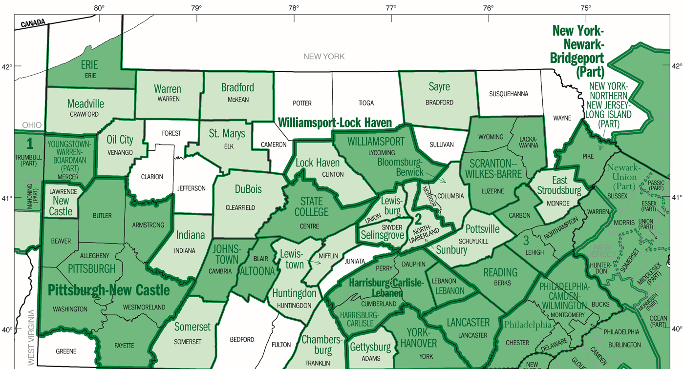
Figure 1. Pennsylvania – Core-Based Statistical Areas and Counties. Source: 2002 Economic Census, U.S. Census Bureau.
Recent studies have shown that perception of climatic variability does get capitalized into farmland values and other assets (Severen, Costello, and Deschenes Reference Severen, Costello and Deschenes2016, Bunten and Kahn Reference Bunten and Kahn2017, Haddon Reference Haddon2017).To measure the impact of expected climatic variability on farmland values, two lagged weather variables of the growing season (April to October) are used: monthly mean temperature (mntm) and total precipitation level in the growing season (tpcp) from the previous year. These two variables serve as a simple forecast for climatic variability. Both variables are computed from the original monthly weather station data provided by the National Oceanic and Atmospheric Administration (NOAA). For counties with incomplete weather station data during the study period, average values from all of their neighboring counties are used as a proxy.
Estimation
The benchmark model specified in (2) is estimated as a fixed effects panel data model using the least-squares dummy-variable (LSDV) estimator (Hsiao Reference Hsiao2003), which proceeds with a data transformation first to eliminate the fixed effects from the regression equation:
 $$p_{it}^{\rm {^\ast}} = p_{it} - \displaystyle{1 \over T}\sum\limits_{s = 1}^T {\,p_{is}} \quad {\rm and}\quad X_{it}^{\rm {^\ast}} = X_{it} - \displaystyle{1 \over T}\sum\limits_{s = 1}^T {X_{is}}.$$
The LSDV estimators of β and σ2 are given by:
 $${\hat {\rm \beta}} _{{\rm LSDV}} = (X^{{\rm {^\ast}}T}X^{\rm {^\ast}})^{ - 1}X^{{\rm {^\ast}}T}p^{\rm {^\ast}}, $$
 $${\hat {\rm \sigma}} ^2_{{\rm LSDV}} = (\,p^{\rm {^\ast}} - X^{\rm {^\ast}}{\hat {\rm \beta}} _{{\rm LSDV}})^T(\,p^{\rm {^\ast}} - X^{\rm {^\ast}}{\hat {\rm \beta}} _{{\rm LSDV}})/(NT - N - K), $$
and
 $${\rm Var}({\hat {\rm \beta}}_{\rm LSDV}) = {\hat {\rm \sigma}}_{\rm LSDV}^{2} (X^{{\ast}T}X^{\ast})^{ - 1},$$
where K is the number of explanatory variables in X. In a random effects model, αi is treated as a random variable that satisfies  ${{\rm \alpha} _i} \; {\sim} \; {\rm I}{\rm. I}{\rm. D}{\rm.} \lpar 0\comma \; {\rm \sigma} _{\rm \alpha} ^2 \rpar $. If αi is further assumed to be independent from εit, letting ωit = αi + εit, a feasible generalized least squares (FGLS) estimator of the random effects model can be given by (Wooldridge Reference Wooldridge2010):
 $${\hat {\rm \beta}} _{{\rm FGLS}} = (X^T{\hat {\rm \Omega}} ^{ - 1}X)^{ - 1}X^T{\hat {\rm \Omega}} ^{ - 1}p, $$
where  ${\hat {\rm \Omega}} = {\hat {\rm \sigma}} ^2I_T + {\hat {\rm \sigma}} _\alpha ^2 e_Te_T^T $, with e T being a T × 1 vector of ones. ${\hat {\rm \sigma}} ^2$ and ${\hat {\rm \sigma}} _{\rm \alpha} ^{\rm 2} $ here are estimated first using ordinary least squares (OLS) regression with pooled data (Wooldridge Reference Wooldridge2010). The variance of ${\hat {\rm \beta}} _{{\rm FGLS}}$ is given in the usual FGLS form:
 $${\rm Var}\lpar {\hat {\rm \beta}} _{{\rm FGLS}}\rpar = {\hat {\rm \sigma}} ^2\lpar X^T{\hat {\rm \Omega}} ^{ - 1}X\rpar ^{ - 1}.$$
Based on the estimates from (18), (20), (21), and (22), the Hausman test is used to decide whether a fixed effects model or random effects model should be used. The estimation results are reported in Table 2, with the test suggesting that the fixed effects model is preferred. The fixed effects specification is also known to be robust against the possible correlation of αi with included regressors in the model, as well as robust against the spatial specification of αi (Lee and Yu Reference Lee and Yu2010a).
Table 2. Estimates with Dependent Variable as GDP Deflated Farmland Values

Note: asterisks (*,**,***) indicate estimate significance at 10 percent, 5 percent, and 1 percent confidence level, respectively.
Before estimating the fixed effects spatial lag model in (7), the semiparametric procedure outlined in the spatial weights matrix section is used to produce a consistent estimate of W N. The second stage substitutes the estimated value of W N,  $\hat W_N$ from the first stage, into (7) and estimates the following model:
 $$p = {\rm \rho} \lpar I_T \otimes \hat W_N\rpar p + \lpar \iota _T \otimes {\rm \alpha} \rpar + X{\rm \beta} + {\rm \varepsilon} {\rm.} $$
The model in (23) is estimated via maximum likelihood estimation (MLE) with the concentrated log-likelihood function proposed by Elhorst (Reference Elhorst, Fischer and Getis2010), which is shown to be equivalent to the original log-likelihood function in terms of estimating β, ρ, and σ2. Assuming normally distributed error term ε, and using the same data transformation as in (17), the concentrated log-likelihood function is given by:
 $$\eqalign{{\rm Log}L & = - \displaystyle{{NT} \over 2}{\rm log}\lpar 2{\rm \pi} {\rm \sigma} ^2\rpar + T\; {\rm log}\left \vert {I_N - {\rm \rho} {\hat W}_N} \right \vert \cr & - \displaystyle{1 \over {2{\rm \sigma} ^2}}\sum\limits_{i = 1}^N {\sum\limits_{t = 1}^T {{\left({\,p_{it}^{\rm {^\ast}} - {\rm \rho} \sum\limits_{\,j = 1}^N {{\hat W}_{ij}p_{\,jt}^{\rm {^\ast}} - X_{it}^{\rm {^\ast}} {\rm \beta}}}\right)}^2}}.}$$
As shown by Lee and Yu (Reference Lee and Yu2010a, Reference Lee and Yu2010b), direct estimation using the log-likelihood function in (24) produces inconsistent estimate of σ2 when T is small and N is large, and therefore a bias correction procedure based on data transformation is proposed. This study incorporates Lee and Yu (Reference Lee and Yu2010a, Reference Lee and Yu2010b)’s data transformation procedure.
The estimate of spatial weights matrix  $\hat W_N$ is obtained semiparametrically via polynomial expansion, with six expansion terms on distance measure d ij (i.e., k n = 6). Here d ij is defined as following:
 $$d_{ij} = A_{\,j}W_{ij}\;{\rm and}\;W_{ij} = \left(\matrix{{1,} \hfill & {\rm if}\;{\rm county}\;i\;{\rm and}\;j\;{\rm share}\;{\rm border} \hfill \cr {0,} \hfill & {\rm otherwise} \hfill \cr } \right.$$
where A j is the normalized (to [0, 1]) total farmland area (average over 7 census years) in county j, and being used as a weight on the binary (0, 1) distance measure. Note that, computationally, if no weights are used in (25) (i.e., d ij = W ij) then the semiparametric estimate  $\hat W_N$ is identical to W (0,1), after both being row standardized,Footnote 2 W (0,1) stands for the spatial weights matrix specified based on binary (0, 1) spatial contiguity. This equivalence only happens when d ij is a single measure and d ij = W ij. The idea of constructing d ij this way is to directly compare the difference between an estimated weights matrix and a prespecified weights matrix. In other words, it is important to examine how the proposed semiparametric procedure can improve the model performance.
Figure 2 plots the row standardized W A = [d ij], farmland area weighted contiguity weights matrix, and  $\hat W_N$. Note that, by construction, the two weights matrices have the same set of nonzero elements, which makes them comparable directly. The difference between the two plots shows refinement through the proposed semiparametric procedure. It is clear that the estimated matrix $\hat W_N$ is more sparse than W A. The sparsity measures also show a substantial difference between the two (5.4167 vs. 10.7218), computed as the sum of squared deviations from the mean (of all nonzero elements).

Figure 2. Comparison of Spatial Weights Matrices.
As previously pointed out, the main concern in estimating the spatial weights matrix W from (10) is the endogeneity in price variables. In this study, the instruments used for farmland prices are one-year lagged HPIs from the nearest MSA. It is the same set of 16 MSAs used for constructing the price uncertainty variables. There are two motivations for using HPIs as the instruments. First, HPIs are highly correlated with farmland prices across the entire state, given that the set of 16 MSAs spreads across the state (Figure 1). Except at some urban-fringe area, it is unlikely that the unobservables driving farmland values also significantly affect the housing prices in metropolitan areas. Second, the literature has shown that farmland has produced high returns with moderate volatility, while most equities (including real estate) had low returns with high volatility in recent decades, suggesting that farmland investments significantly improve the risk-efficiency of mixed-asset portfolios (Hennings, Sherrick, and Barry Reference Hennings, Sherrick and Barry2005). The relatively weak linkage between farmland and real estate investments and the exogeneity created by the one-year lag validate the instruments. An alternative is to use lagged farm characteristics as instruments. However, this more likely causes a weak instrument issue, given that these variables are used as explanatory variables in the second step estimation (Murray Reference Murray2006).
Results and Discussion
Estimation results under different model specifications are summarized in Table 2. The first result to examine is the evidence of spatial dependence. Both spatial lag fixed effects models give significant estimates on the spatial autoregressive parameter ρ, 0.5360 and 0.5030, respectively. The existence of spatial interdependence in the hedonic pricing model can be interpreted as the spatial simultaneity of farmland values observed across counties.
By simply comparing the likelihood values, the model with the estimated weights matrix  $\hat W_N$ fits better than with the farmland area weighted contiguity weights matrix W A. In general, the model goodness of fit is measured by the information criterion (e.g., AIC, BIC). In this paper, however, two spatial models with different weights matrices are not nested. Therefore, the information criterion does not apply to model comparison directly. Another thing to consider is that the proposed approach proceeds in two steps, which affect the degree of freedom in the estimation. Instead, the Voung test (Voung Reference Vuong1989) and the distribution-free test for non-nested model selection developed by Clarke (Reference Clarke2007) are employed to decide if the proposed approach should be statistically preferred. Test results are reported in Table 3.
Table 3. Goodness of Fit Across Spatial Dependence Structures (Spatial Lag FE Model)

Though the true model is unknown to the researcher, both tests reject the null hypothesis that two rival models are equally close to the true specification. The proposed model, motivated by economic theory, is statistically preferred. An alternative way to gauge the robustness of the proposed approach is through out-of-sample prediction. To do so, the spatial lag fixed effects model is estimated using data from 1982 to 2007 with weights matrices W A and  $\hat W_N$, respectively. The estimated coefficients and fixed effects are then used to predict farmland values in 2012. Figure 3 compares two different predictions, with the blue (dark) line being a 45-degree line. According to the computed sum of squared errors of prediction (SSE), the model with weights matrix $\hat W_N$ reduces SSE by 16.4 percent (from 26.0027 to 21.7412). Overall, both models underpredict 2012 farmland values, which may be explained by the farmland boom around 2012.

Figure 3. Out-of0Sample Predictions of 2012 Farmland Values.
LeSage and Pace (Reference LeSage and Pace2009) suggest that it is necessary to obtain an unbiased measure of the marginal effect of an explanatory variable in spatial models. As shown in LeSage and Pace (Reference LeSage and Pace2009), computation of marginal effects should take into account both the direct effect and the indirect effects through the spatial interactions and simultaneous feedback in the model structure. From (7), given any time period t = t 0, it follows that
 $$\displaystyle{{\partial p} \over {\partial X_k}} \vert _{t = t_0} = {\rm \beta} _k\lpar I_N - {\rm \rho} W_N\rpar ^{ - 1}.$$
The derivative in (26) is time-invariant. The total marginal effect is given by taking average of all cross-section units:
 $$N^{ - 1}\sum\limits_{i = 1}^N {\sum\limits_{\,j = 1}^N {\displaystyle{{\partial p_i} \over {\partial X_{\,jk}}} = {\rm \beta} _kN^{ - 1}[{\iota} ^{\prime}{(I_N - {\rm \rho} W_N)}^{ - 1}\iota ]}}, $$
where  $\iota $ is a N × 1 vector of ones. The direct effect is given by only averaging over the diagonal elements:
 $$N^{ - 1}\sum\limits_{i = 1}^N {\displaystyle{{\partial p_i} \over {\partial X_{ik}}} = {\rm \beta} _kN^{ - 1}\; {\rm trace}[{\lpar I_N - {\rm \rho} W_N\rpar }^{ - 1}]}.$$
 As pointed out by LeSage and Pace (Reference LeSage and Pace2009), the direct effect is different from the coefficient estimate  ${ \hat {\rm \beta}} _k$ because of the spatial autoregression process among dependent variables observed at different cross-section units. Table 4 presents the direct, indirect, and total effects based on the estimates using spatial lag fixed effects models (Table 2) and the estimated weights matrix $\hat W_N$.
Table 4. Direct, Indirect, and Total Marginal Effects

Note: asterisks (*,**,***) indicate estimate significance at 10 percent, 5 percent, and 1 percent confidence level, respectively.
For log-transformed variables, the computed direct marginal effects in Table 4 can be directly interpreted as price (of farmland) elasticity. The results show both new findings and consistency with the literature. According to the spatial lag FE (2) model in Table 2, significant determinants of farmland value include farm ownerships, operator age, expected growing season temperature, and price uncertainty. Over the three-decade period, the real value of farmland has gone up, as indicated by the time trend estimate (year). Return to agricultural assets (m_sales) has the expected sign but is insignificant.
In terms of magnitude, operator age has the greatest impact on farmland values. A 1-percent increase in principal operator age (a proxy for experience in farming), given a mean value of 53.64, can increase farmland value by more than 1 percent. The percentage of dairy farms (p_dairy) has a negative but insignificant impact, which suggests that on average the pasture land in dairy farms offsets the land appreciation due to extra facilities and structures on dairy farms. The expected precipitation level in growing season has an insignificant effect. The expected growing season temperature level, however, has a significant negative impact on farmland values. Given an average temperature of 16.58 C, a 1-degree (about 6 percent) increase in average temperature could reduce farmland values by 2.77 percent. These findings are qualitatively consistent with the literature on climatic impact on farmland values (e.g., Mendelsohn, Nordhaus, and Shaw Reference Mendelsohn, Nordhaus and Shaw1994, Schlenker, Hanemann, and Fisher Reference Schlenker, Hanemann and Fisher2006).
Two interesting results are the impacts of farmland ownership and price uncertainty. The percentage of fully owned farmland (p_fullown) has a strong positive impact on farmland values. One concern associated with this result is that the p_fullown variable may be endogenous due to the fact that there may be selection effects when allocating farmland between owning and renting. Before addressing this potential endogeneity issue, a good understanding of the determination of farmland ownership is necessary. This points to a fruitful direction for future research. As for the impact of market uncertainty, the results show that the short-run volatility (measured by q4) tends to push up farmland values, while the long-run volatility (measured by q8) does the opposite. In the short run, market volatility can lead to speculation on farmland values among farmers and land developers. In the long run, however, farmers and developers may start acting more conservatively when facing risks.
Given that the time-invariant variables in the fixed effects model are absorbed by fixed effect αi, they are excluded from the spatial lag fixed effects models. One interesting time-invariant determinant of farmland values often explored in the literature is the distance to large metropolitan areas (d_metro). To examine how the distance to the nearest large metropolitan area affects farmland values, a spatial lag random effects model is estimated. The estimated parameter is −0.0416 (s.e. = 0.0255), with total and direct marginal effects being −0.1464 and −0.0487, respectively. This is higher than the estimated elasticity of −0.0280 in Huang et al. (Reference Huang, Miller, Sherrick and Gomez2006) using Illinois data.
How government support and policy affect farmland values is also commonly studied in the literature. This paper uses average government payment received per acre (m_gpay) as a proxy for government support and policy. Because this measure is not available in the Census data before 1987, the spatial lag fixed effects model is re-estimated with a reduced panel of six time periods. The estimated parameter is 0.0526 (s.e. = 0.0173; total marginal effect = 0.0780, direct marginal effect = 0.0538), which implies a $1 increase in government payment can, on average, increase farmland value by $4.2.Footnote 3 The estimate is consistent with findings in the literature (e.g., Weersink et al. Reference Weersink, Clark, Turvey and Sarker1999).
After controlling for spatial heterogeneity and spatial dependence, several explanatory variables (e.g., p_farmarea, farms) become insignificant in the spatial fixed effects model. It suggests that these variables may have picked up certain spatial relationships among farmland values across space. Another noticeable result is the decline of the spatial autoregressive parameter ρ with the estimated weights matrix (Table 3). Given that the weights matrix in MLE is always row standardized first, a possible explanation for this change is that when the spatial weights matrix is poorly specified, the spatial autoregressive parameter ρ could absorb a certain amount of information on the spatial dependence structure. In such cases, ρ plays both the role of measuring the strength of spatial dependence and the role of being a scaling parameter.
Concluding Remarks
One of the main criticisms of spatial econometrics approach is the gap between economic theory and empirical application. As argued by Corrado and Fingleton (Reference Corrado and Fingleton2012), determination of spatial weights matrix should incorporate more economic theory and lead to more structural approach in examining spatial interactions and spillovers. In this study, a spatial hedonic pricing model is estimated with a two-stage procedure which treats the spatial weights matrix endogenously. The first stage follows Pinkse, Slade, and Brett (Reference Pinkse, Slade and Brett2002)’s semiparametric approach to estimate the spatial weights matrix using pooled data, which gives a consistent estimate for the spatial weights matrix backed up by economic theory. The second stage estimates a spatial panel data model with the estimated weights matrix from the first stage. Overall, the proposed approach improves the fit and the predictability of farmland valuation models.
The empirical results show both new findings and consistency with the literature. The first key result is the evidence of strong spatial dependence. In the spatial autoregressive framework, farm ownership, operator's age, expected growing season temperature, price uncertainty, government payment, and distance to the nearest metropolitan area are found among key determinants of farmland values. The evidence of strong spatial dependence among farmland values also carries important policy implications. To avoid potential tax distortion and its impacts on the local economy, for example, accurate farmland valuation is fundamentally important in land-related tax assessment. Distortionary taxation could potentially direct capitals to competing jurisdictions and lead to deterioration of local farmland market.
The spatial panel hedonic pricing model can account for spatial-temporal relationships and be used to control for spatial heterogeneity to some extent. To fully model the temporal dynamics in farmland market, a forward-looking structural dynamic model is necessary, which usually requires individual farm-level data and is out of the scope of this paper. The approach in this paper is subject to certain limitations. This study uses county-level aggregate data, which may cause issues when farmland valuation function has essentially different structures among different categories of farmland (e.g., crop farming vs. livestock farming). Under these circumstances, an aggregate valuation function may not exist, and estimates of aggregate coefficients may not have expected interpretation (Pinkse and Slade Reference Pinkse and Slade2010). This study uses panel data over a relatively short time period T, therefore the spatial weights matrix can be estimated with pooled data without much concern about structural change in the agricultural sector. The proposed first stage may no longer be sufficient when T gets larger; in that case, a time-varying spatial weights matrix should be considered (Lee and Yu Reference Lee and Yu2012). Such kind of methodological concerns need to be focused in further research.
Financial Statement
There is no funding support for this research.


 Open access