


1. INTRODUCTION
In recent years there has been a decrease in the Arctic sea-ice cover (e.g. Stroeve and others, Reference Stroeve, Holland, Meier, Scambos and Serreze2007) which has lead to increased ship traffic and other operations in the Arctic. In order to travel and operate safely in the Arctic, there is a need for high-quality Arctic sea-ice forecasts.
There are several advanced sea-ice models currently in use for modelling sea-ice, for example the Louvain-la-Neuve sea-ice model (LIM3; Vancoppenolle and others, Reference Vancoppenolle2009) and the Los Alamos sea-ice model (CICE; Hunke and Dukowicz, Reference Hunke and Dukowicz2002). Also, several fully coupled models with integrated sea-ice components have been developed, for example the Massachusetts Institute of Technology General Circulation Model (MITgcm; Marshall and others, Reference Marshall, Adcroft, Hill, Perelman and Heisey1997; Losch and others, Reference Losch, Menemenlis, Campin, Heimbach and Hill2010), towards an Operational Prediction system for the North Atlantic European coastal Zones (TOPAZ; Sakov and others, Reference Sakov2012) and the Community Ice-Ocean Model (CIOM; Yao and others, Reference Yao, Tang and Peterson2000). These models are the most commonly used for sea-ice modelling, and they all use the elastic-plastic-viscous rheology (Hunke and Dukowicz, Reference Hunke and Dukowicz1997, Reference Hunke and Dukowicz2002) based on former schemes using the viscous-plastic rheology (Hibler, Reference Hibler1979).
Since the late 1970s, the amount of observable meteorological variables has increased significantly due to the development of satellite technology. This has led to new and improved techniques for assimilation of observations in numerical models. The first approaches used in numerical meteorology were simple interpolation methods (Panofsky, Reference Panofsky1949; Barnes, Reference Barnes1964; Hoke and Anthes, Reference Hoke and Anthes1976). Later more advanced mathematical methods were introduced, such as the 3D-variational methods (3D-Var; Sasaki, Reference Sasaki1970) and the 4D-Var (Dimet and Talagrand, Reference Dimet and Talagrand1986; Bouttier and others, Reference Bouttier, Derber and Fisher1997), where 4D-Var is a further development of 3D-Var, taking the variation of observations with time into account by assimilating at the time of observation. The 4D-Var assimilation requires a tangent linear and adjoint model that is run several times both backward and forward in time. The tangent linear and adjoint models can be difficult to develop, and the assimilation is computationally expensive since it requires several backwards and forwards operations. Later Evensen (Reference Evensen1994) introduced the ensemble Kalman filter (EnKF; Evensen, Reference Evensen1994, Reference Evensen2003, Reference Evensen2009; Burgers and others, Reference Burgers, van Leeuwen and Evensen1998) as an alternative to the variational methods, where cross-covariances are continuously updated based on the statistics of an ensemble of model states. These assimilation methods have been extensively used in a wide range of applications, especially for NWPs (e.g. Evensen, Reference Evensen2003; Gauthier and others, Reference Gauthier, Tanguay, Laroche, Pellerin and Morneau2007; Houtekamer and Zhang, Reference Houtekamer and Zhang2016).
In the last 30 years, there has been an increase in Arctic observations due to an increased number of polar-orbiting satellites. This has lead to several attempts at assimilating sea-ice concentration (SIC) observations. SIC is defined as the fraction of the geographical area covered by sea ice. Lisæter and others (Reference Lisæter, Rosanova and Evensen2003) were pioneers within SIC assimilation. In their study, the EnKF was used to assimilate SIC from passive microwave-sensor data into a coupled sea-ice ocean model. The assimilation was found to improve the modelled SIC compared with observations, especially along the ice edge. The effect of assimilation was found to be stronger in summer compared with winter, partly due to lower ensemble spread in winter causing excessive confidence in the model, and partly due to larger differences between the modelled SIC and observed SIC in summer. The result also showed an improved model estimate of sea-ice thickness (SIT) caused by multivariate update during the assimilation.
Caya and others (Reference Caya, Buehner and Carrieres2010) used CIOM (Yao and others, Reference Yao, Tang and Peterson2000) and the 3D-Var assimilation method to assimilate daily gridded ice charts covering the Canadian east coast. In this study, 3D-Var assimilation was compared with a direct insertion method and a nudging method using short-term forecasts. The three methods showed similar skilful short-term forecasts when the daily ice charts were assimilated. When SIC observations from Radarsat were included in the assimilation, the 3D-Var method was found to give significantly improved results compared to ignoring the observations, demonstrating the advantage of 3D-Var to simultaneously assimilate multiple types of observations.
The TOPAZ4 system is a coupled sea-ice ocean data assimilation system for the North Atlantic and the Arctic. In TOPAZ4 both ocean and ice observations are assimilated using the EnKF. Previous experiments with the TOPAZ4 system have shown good multivariate impact of SIC assimilation (Sakov and others, Reference Sakov2012). Similar experiments showing multivariate update of sea-ice parameters for SIC assimilation were done with the NEMO-LIM3 model (Massonnet and others, Reference Massonnet, Fichefet and Goosse2015). Both studies showed model improvements of SIT as a consequence of SIC assimilation.
Lindsay and Zhang (Reference Lindsay and Zhang2006) and Wang and others (Reference Wang, Debernard, Sperrevik, Isachsen and Lavergne2013) used nudging methods to assimilate SIC into coupled sea-ice ocean models. Wang and others (Reference Wang, Debernard, Sperrevik, Isachsen and Lavergne2013) used the Combined Optimal Interpolation and Nudging (COIN) method to assimilate SIC based on SSM/I observations (OSISAF, www.osi-saf.org) into the ROMS model (Shchepetkin and McWilliams, Reference Shchepetkin and McWilliams2005). The results were validated against the AMSR-E SIC maps acquired from microwave scanning radiometer (Spreen and others, Reference Spreen, Kaleschke and Heygster2008), and it was found that the assimilation induced a significant improvement of the background model. Lindsay and Zhang (Reference Lindsay and Zhang2006) assimilated the Gice SIC dataset (Rayner and others, Reference Rayner, Horton, Parker, Folland and Hacket1996) into a coupled sea-ice ocean model. Significant multivariate improvements were found by validation against upward-looking sonar observations of ice draft.
Recent developments in satellite technology and measurement techniques have led to the possibility of observing SIT from satellites. The first experiment with SIT observations was done by Lisæter and others (Reference Lisæter, Evensen and Laxon2007). They assimilated synthetic SIT observations and found multivariate effects on ocean salinity, surface temperature and SIC. Today SIT observations are available from the European Spaces Agency's (ESA) Cryosat and Soil Moisture and Ocean Salinity (SMOS) missions. The SMOS dataset includes observations of SIT reliable for thicknesses smaller than 0.4 m (Xie and others, Reference Xie, Counillon, Bertino, Tian-Kunze and Kaleschke2016). These data have recently been introduced in the TOPAZ4 assimilation system, and it was found that assimilation of the SMOS thickness provides significant improvements on the thin SIT and slight improvements to the SIC (Xie and others, Reference Xie, Counillon, Bertino, Tian-Kunze and Kaleschke2016).
There are several challenges regarding sea-ice assimilation, such as the lack of routinely observed parameters other than SIC. Thickness can be observed, yet the reliability is limited. The SIC forecast is strongly dependent on both SIT and sea-surface temperature (SST), thus assimilation with a multivariate approach is essential. However, SIC is a bounded variable between zero and one. Therefore, a SIC of one may be related to any thickness, and a SIC of 0 can, in principle, mean an SST of anything from − 1.8K and warmer. The EnKF has large technical advantages compared with the nudging methods, for example by spreading the information in space and across variables. Still, when the EnKF is applied to bounded parameters such as SIC, the EnKF may fail to show improved skills relative to the simpler approaches.
This study introduces a multi-variate nudging (MVN) method, which is an improvement of the simple 1D-nudging method (Wang and others, Reference Wang, Debernard, Sperrevik, Isachsen and Lavergne2013). The improvements consist of a multivariate and spatially updating mode.
In the next section, the assimilation systems for MVN and EnKF based on the state-of-the-art sea-ice model CICE version 5.1 are introduced. In the results section, the MVN method is compared with the more advanced EnKF in terms of spatial and multivariate update associated with assimilation of SIC and SIT.
2. ASSIMILATION SYSTEM
2.1. The CICE model
The Los Alamos CICE model version 5.1 (Hunke and Dukowicz, Reference Hunke and Dukowicz2002) is a state-of-the-art sea-ice model using the elastic-plastic-viscous rheology (Hunke and Dukowicz, Reference Hunke and Dukowicz1997). The model has components for thermodynamics, dynamics, transport and ridging. The model uses five SIT categories, with seven ice layers and one snow layer. CICE is a computationally efficient model and is used in fully coupled models, for example Community Earth System Model (CESM; Hurrell and others, Reference Hurrell2013). The CICE model is used in the present study for modelling the sea ice.
2.2. Forcing data
In our study, the CICE model is forced by atmospheric data and SST from the ERA-Interim dataset of the European Centre for Medium Ranged Weather Forecast (ECMWF; Dee and others, Reference Dee2011). Sea-surface salinity (SSS) is taken from the Regional Ocean Modelling System, Arctic-20 km (ROMS; Shchepetkin and McWilliams, Reference Shchepetkin and McWilliams2005). Data from ROMS were only available from 2010 to 2013, these data have been applied in a perpetual way in order to spin-up the model. The atmospheric forcing used is precipitation, cloud cover, moisture content and 2 m air temperature from the ERA-Interim dataset. The SST forcing has been modified to be consistent with the observations: every grid point where the observations indicate SIC larger than 0.1 has been set to the mushy freezing point defined by the CICE model. This model freezing point, T f [°C], is a function of the salinity, S, defined by,
 $$T_{\rm f} = \displaystyle{S \over { - 18.48 + \left( {18.48 \times 0.001S} \right)}}.$$
2.3. Observations
In the present study, the re-analyzed SIC product from the European Organization for the Exploitation of Meteorological Satellites (EUMETSAT) Ocean and Sea Ice Satellite Application Facility (OSISAF, www.osi-saf.org) is used for assimilation (Tonboe and others, Reference Tonboe, Lavelle, Pfeiffer and Howe2016). The OSISAF dataset is based on SSM/I observations of antenna temperatures converted into brightness temperatures, and then corrected for atmospheric contamination by the ECMWF NWP model (Andersen and others, Reference Andersen, Tonboe, Kern and Schyberg2006). The brightness temperatures are then converted into SIC by a combination of the Bootstrap algorithm (low concentration) and the Bristol Algorithm (high concentration; Tonboe and others, Reference Tonboe, Lavelle, Pfeiffer and Howe2016). The OSISAF dataset includes an observation confidence, C, given on a scale between zero and five, where five indicates a high confidence and zero indicates no confidence. Based on estimates of representativeness uncertainty, observation operator uncertainty and measurement uncertainty, we have chosen a minimum observation uncertainty of 0.1 for the OSISAF SIC observations. Additionally, we chose a linear increase of uncertainty with decreasing confidence of the observation. The observation uncertainty, σobs based on these assumptions is defined as,
 $$ \sigma_{{\rm obs}} = 0.1(6-C). $$
For the open ocean and the ice interior the observation confidence is high (five), while in/around the marginal ice zone the confidence varies between one and four. The OSISAF dataset is structured on a 10 km stereographic grid, using a Gaussian weighting with 75 km radius of influence for each observation. Coastal regions and fjords are masked out in the OSISAF dataset (Tonboe and others, Reference Tonboe, Lavelle, Pfeiffer and Howe2016).
In the present study, the observations of SIT are the SMOS daily SIT (Tian-Kunze and others, Reference Tian-Kunze2014) version 3.1. The SMOS dataset consists of microwave measurements (L-band) of brightness temperatures converted into SIT by applying a radiation model and a thermodynamic model, the full algorithm used for the conversion is described by Tian-Kunze and others (Reference Tian-Kunze2014). Following Xie and others (Reference Xie, Counillon, Bertino, Tian-Kunze and Kaleschke2016), only ice thinner than 0.4 m has been used in the analysis. Therefore, the observations are sparse and they vary in location and on a daily basis. All observations include an uncertainty estimation which is used to define the observation impact during assimilation. Due to wet snow conditions and melt ponds on the sea ice in summer, it is currently not possible to accurately calculate the SIT in this season. Thus the SMOS dataset is only available in the cold season from mid-October to mid-April from 2010 to present. The SMOS observations are structured on a stereographic grid with 12.5 km resolution.
2.4. Ensemble Kalman Filter
The EnKF is a sequential data assimilation method used in a wide variety of geophysical systems (Evensen, Reference Evensen1994, Reference Evensen2009; Houtekamer and Zhang, Reference Houtekamer and Zhang2016). The key property of the EnKF is that the model uncertainty is calculated from an ensemble of model states, generated by perturbing the forcing, the model parameters, the observations or a combination of the three. The Kalman filter equation can be written as (Jazwinski, Reference Jazwinski1970; Evensen, Reference Evensen2003),
 $$ \vec{\phi}^{{\rm a}}=\vec{\phi}^{{\rm f}}+\vec{P}^{{\rm f}}\vec{H}^{T}\left(\ \vec{HP}^{{\rm f}}\vec{H}^{T} + \vec{R} \right)^{-1} \left( \vec{d} - \vec{H}\vec{\phi}^{{\rm f}} \right). $$
In this equation,  $\vec {\phi }^{{\rm f}}$ ∈ ℝn×N and $\vec {\phi }^{{\rm a}}$ ∈ ℝn×N are the model first guess and analysis state vector, respectively. In the state vector, all information about the current state of the model is stored. Here n is the number of variables multiplicated by the number of grid points, and N is the number of ensemble members. The co-variance of observations is given by $\vec {R}$ ∈ ℝm×m, where m is the number of observations, $\vec {H}$ ∈ ℝm×n is the transformation matrix operator used to transform the model to observation state space, $\vec {d}$ ∈ ℝm×N represents the observations. The estimated model co-variance, $\vec {P}^{{\rm f}}$ ∈ ℝn×n, is given by,
 $$ \vec{P}^{{\rm f}} = \overline{ (\vec{\phi}^{{\rm f}} - \overline{\vec{\phi}^{{\rm f}}}) (\vec{\phi}^{{\rm f}} - \overline{\vec{\phi}^{{\rm f}}}) }. $$
In (4) the overbars indicate ensemble average. The covariance between the different model variables is used to update also non-observed variables. Thus the full state space  $\vec {\phi }^{{\rm f}}$, including all model variables, can be updated based on observations of a single variable.
The EnKF analysis may lead to spurious co-variances caused by distant state vector elements and insufficient model rank when small ensemble sizes are used. These artefacts can be reduced by using a method for localization (Evensen, Reference Evensen2003; Sakov and Bertino, Reference Sakov and Bertino2011). With localization, the analysis is limited to local areas. In our study, the polynomial taper function by Gaspari and Cohn (Reference Gaspari and Cohn1999) was used to create a smooth localization where nearby grid points are more important than distant grid points in the analysis.
In the present study, the deterministic EnKF (DEnKF) was used. This method has been shown to perform better for ensemble prediction systems with few ensemble members (Sakov and Oke, Reference Sakov and Oke2008). The code used for assimilation is the EnKF-c algorithm version 1.60.3 ().
An example of the EnKF assimilation is given in Fig. 1. In this figure, an average of all ensemble members is given before and after EnKF assimilation for the difference between modelled (CICE) and observed (OSISAF) SIC on 23 October 2011. The largest differences after assimilation are located in the marginal ice zone, where the ensemble spread is largest, and therefore, the observations have the largest impact on the EnKF assimilation. Note that since concentration is a bounded value, no errors are expected in the ice interior where both observations and model have a concentration of 1. Thus, it is clear that the effect of assimilation varies throughout the Arctic, some locations show large impacts of assimilation, while others have little impact. This reflects the robustness of the EnKF and demonstrates how ensemble spread is used in the EnKF to update the model.
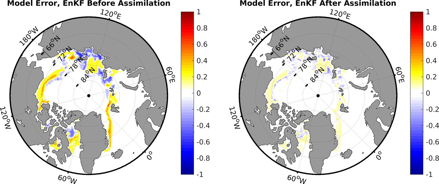
Fig. 1. Difference between modelled (CICE) and observed (OSISAF) SIC on 23 October 2011, before (left) and after (right) assimilation using EnKF.
2.5. Multivariate nudging
The COIN is a basic data assimilation method where model variables are nudged towards observed values based on an optimal interpolation between model and observations. The model uncertainty in the COIN scheme is dependent on the difference between model and observation. The basic formulation of the MVN method used in the present study is similar to the COIN method applied by Wang and others (Reference Wang, Debernard, Sperrevik, Isachsen and Lavergne2013). We use a slightly altered nudging weight, and assimilation is done at 10-day intervals. The assimilation time step is chosen to be similar to that applied in the EnKF. For the EnKF assimilation, the build-up of ensemble spread requires a sufficient time period between assimilation steps. We used 10 days to compensate for a stand-alone model with decreased model drift caused by a prescribed ocean component. The major difference between the methods of MVN and COIN is that multivariate and spatial properties have been included for MVN. The assimilation process for the MVN and COIN is given by
 $$ \phi^{{\rm a}}_{i} = \phi^{{\rm f}}_{i} + G_{i}\left(d_{i} - \phi^{{\rm f}}_{i}\right) $$
In this equation all variables are scalars,  $\phi ^{{\rm a}}_{i}$ and $\phi ^{{\rm f}}_{i}$ are the analysis and model first guess, respectively, d i represents the observed value, and G i is the nudging weight. The subscript i indicates a specific grid point, which from here on will be omitted. In order to make the results from the analysis comparable with those of the EnKF, the observed value d is perturbed using a normal distribution with a mean of zero and a standard deviation equal to the observation uncertainty σ obs. The nudging weight is defined as
 $$ G = K/\tau, $$
where,
 $$K = \displaystyle{{\sigma _{\rm m}^2 } \over {\sigma _{\rm m}^2 + \sigma _{{\rm obs}}^2 }},$$
and  $\sigma _{{\rm {\rm m}}}$ and σ obs represent the model and observation uncertainty, respectively. The τ parameter is a delay timescale of the nudging towards observations. τ is defined such that large uncertainties have less delay,
 $$ \tau = \exp{a(\sigma_{{\rm max}}-\sigma_{{\rm m}})}. $$
In Eqn (8) the parameter a is a nudging delay parameter defining the strength of the nudging, and σmax is the largest possible uncertainty, for example unity for SIC, in the present study we used a equal to one. The model uncertainty is defined as the difference between the observation and the model first guess:
 $$ \sigma_{{\rm m}} = \vert d - \phi^{{\rm f}} \vert $$
The observation uncertainty, σ obs, is taken from the confidence levels of the observations, given by Eqn (2).
In the study by Wang and others (Reference Wang, Debernard, Sperrevik, Isachsen and Lavergne2013) the modelled SIT was preserved during assimilation. When new ice was added as a result of the assimilation, the ice thickness was enforced to be 0.5 m. In the present study, we use an alternative approach where a statistical relationship between ice volume and SIC is used for the multivariate update. This approach is based on observation statistics from the marginal ice zone. The CICE model does not use SIT directly but calculates SIT as the sea-ice volume divided by the SIC. Thus the sea-ice volume must change when the SIC changes to preserve model physics after assimilation. For example, if the SIC is reduced during assimilation and the modelled ice volume is unchanged, the resulting ice would be thicker. Thick ice is more resistant to melt and will cause a build-up of ice at the ice edge. Similarly, increased SIC will result in thin ice which requires less energy to melt. We used a relationship between ice volume (V) and SIC (C) based on regression of observed SIC (OSISAF) and SIT (SMOS) values (see Fig. 2),
 $$C(V) = \left\{ {\matrix{{12.3\,V,} \hfill & {\lt 0.03,} \hfill \cr {\displaystyle{1 \over {3.867}}\ln \left( {\displaystyle{V \over {0.0072}}} \right),} \hfill & {0.03 \lt V \lt 0.34,} \hfill \cr {1,} \hfill & {V \gt 0.34.}\hfill \cr} } \right.$$
Similarly, when assimilating concentration, (Fig. 3),
 $$V(C) = \left\{ {\matrix{ {0.02C\exp \left( {2.8767C} \right),} \hfill & {0 \lt C \lt 0.8,} \hfill \cr {0.5C,} \hfill & {C \lt 0.8,\,\,V_{\rm m} \lt 0.1.} \hfill \cr} } \right.$$
Fig. 2. Observations of thickness (SMOS) and concentration (OSISAF) spanning the period 2010---12, are used to obtain a relationship between volume and concentration by regression. A random selection of 5000 observations from all available observations is shown. The figure shows concentration as a function of volume. The red dots represent observations and the blue line is the regression line.

Fig. 3. As Fig. 2, but volume as a function of concentration.
The expressions in (10) and (11) are only valid for the marginal ice zone where thickness data are available for regression. When the SIC is close to one, it is not possible to define a relationship between SIC and SIT since SIC is bounded. The model uncertainty in the marginal ice zone is large due to small perturbations inducing transitions between ice and water. These transitions are strongly affected by the forcing, while in the interior of the ice the model is more stable. The second expression in Eqn (11) uses the first guess volume  $V_{{\rm {\rm m}}}$, this ensures that new ice witha high concentration (C > 0.8) resulting from assimilation is coupled to an updated volume, even though this new ice is not located in the marginal ice zone. The two expressions in Eqns (10) and (11) are not the inverse of each other, this is related to minor mathematical simplifications in order to keep the relationships simple.
We used an extrapolation method to improve the spatial properties of the MVN. The extrapolation is performed using a simple digital inpainting approach based on elliptic partial differential equations (). In the present study, a method using the fourth partial derivatives was used.
An example of the MVN assimilation is given in Fig. 4. The figure shows the difference between modelled (CICE) and observed (OSISAF) SIC on 23 October 2011. After assimilation (right panel), the model has been nudged towards observations, by decreasing the difference between model and observations. There are several negative differences in the central Arctic after assimilation. This is due to modelled grid points with lower concentration compared with the observations. These negative values are an artefact of the observation perturbation, which causes small errors at random grid points in the interior of the sea ice. There are only negative differences because the observations are close to the one in the central Arctic and concentrations have an upper bound of 1. Similar errors are not found in the open ocean because the open ocean observations with maximum confidence are not perturbed which avoids ice residuals in known ice-free areas.

Fig. 4. Difference between modelled (CICE) and observed (OSISAF) SIC on 23 October 2011, before (left) and after (right) assimilation using MVN.
3. SETUP
The model simulation was initialized without Arctic sea ice and spun-up without assimilation from 1 January 1979 until 1 January 2010. Both assimilation schemes were then run for 3 years from 1 January 2010 to 31 December 2012 with the assimilation of OSISAF SIC every 10 days. In addition, the assimilation was run for two cold seasons from 15 October 2010 to 15 April 2011, and 15 October 2011 to 15 April 2012 for SMOS SIT assimilation. The number of ensemble members for the EnKF was 20, and a localization radius of 300 km was used. The initial ensemble was generated by using ice states from 1 January from 20 different years. The ensemble members were perturbed in a similar way as used in the TOPAZ system (Sakov and others, Reference Sakov2012), using a smooth pseudo-random field (Evensen, Reference Evensen2003) with zero mean to perturb the input forcing. The standard deviation of temperature used to perturb the 2 m temperature was 10 K. We chose 10 K to compensate for the lack of perturbation in the ocean forcing. The standard deviation for cloud cover was 20%, for the per-area precipitation flux it was 4 × 10⁹ms−1, and for wind, it was 1ms−1. In the CICE model, the shear strength relative to the compressive strength is scaled by the dimensionless parameter e. Since the value of the e parameter is not well known (Dumont and others, Reference Dumont, Gratton and Arbetter2009), we perturbed e to increase the ensemble spread. Following Sakov and others (Reference Sakov2012) we used the parameter e as a normal distributed stochastic variable with a mean equal to two, which is the default model setting and a standard deviation of one.
After assimilation, the state space was post-processed. During the post-processing the variables were checked for physical consistency, to avoid for example hotspots, zero or negative ice volume, snow on water, ice in hot water and similar non-physical situations. For the EnKF assimilation, bounded values such as SIC can create erroneous covariances, which make post-processing important in order to check that variables are within their realistic bounds. For the MVN assimilation, the multivariate update based on the statistical relationship between SIC and SIT was done during the post-processing. When the assimilation resulted in decreased sea-ice extent, the SST were updated to avoid immediate refreezing. This was done by using a predefined gradient of SST based on the distance to the sea-ice edge. The average gradient was estimated from the ECMWF ERA-Interim dataset (Dee and others, Reference Dee2011) to 0.007 Kkm−1. Similarly, when the assimilation provided more sea ice than in the first guess, both the SST and SIT was updated to avoid immediate remelting of the ice.
In the CICE model, the ice is distributed in five thickness categories, while observations only have one category. For the EnKF, this is not a problem, since the individual categories are updated based on the correlation. For the MVN we used the model thickness distributions of the initial first guess to redistribute the assimilation result into the five ice thickness categories. Thus the fraction of the total SIC in a given category was the same before and after assimilation, but the total SIC could have changed. If thickness categories proved to be overfull in the model after assimilation, the surplus volume was transferred to the next thickness category. This method avoids discontinuities in the sea-ice cover.
To analyze the strength of assimilation the RMSE between model and observations were used,
 $${\rm RMSE} = \sqrt {\displaystyle{{\sum\nolimits_{i = 1}^m {{(d_i - \phi _i^a )}^2} } \over m}} .$$
This statistic provides the total deviation between the model and observations but does not provide information on over or under extension of sea ice.
4. RESULTS
A verification of the multivariate properties of the MVN and EnKF assimilation systems has been conducted by two cross-validation experiments. In the two experiments either SIT or SIC observations were assimilated, and the non-assimilated SIC or SIT observations were used for verification. For the assimilation systems shown in Fig. 5, SIC observations were assimilated and SIT observations were used for verification. In this figure, the monthly averaged SIT RMSEs over three cold seasons are plotted. Only observations from the marginal ice zone were used. In the marginal ice zone, the ensemble has the largest spread and the EnKF has the largest effect. For MVN, the multivariate relationship between sea-ice volume and SIC is undefined outside the marginal ice zone, see Eqn (11). In the present study, we defined the marginal ice zone as grid cells with SIC <0.8. The marginal ice-zone location differs between the MVN and EnKF model system, therefore two different marginal ice zone definitions were used for the calculations. In Fig. 5 the solid lines indicate a marginal ice zone as defined for the EnKF assimilation model system, and the dashed lines from the marginal ice zone as defined by the MVN model system. All model results indicate an increase of SIT RMSE from October to April. This is a consequence of modelled ice growth being larger than observed ice growth, which is due to a bias in the background forcing, leading to an overestimation of the sea-ice extent. As a consequence of the sea-ice overestimation, the marginal ice zone as defined by the observations is mostly located in the interior of the modelled ice pack. Since the SIT in the interior increases throughout the cold season, the differences between the modelled and the observed SIT are increasing during this season. The temporal increase of SIT RMSE is most apparent in the control run, blue lines in Fig. 5. When assimilation is applied, the temporal effect is significantly reduced, both for the EnKF and the MVN. However, a small increase of SIT RMSE during the cold season is still evident after assimilation, which is related to the prescribed model forcing not affected by the assimilation.
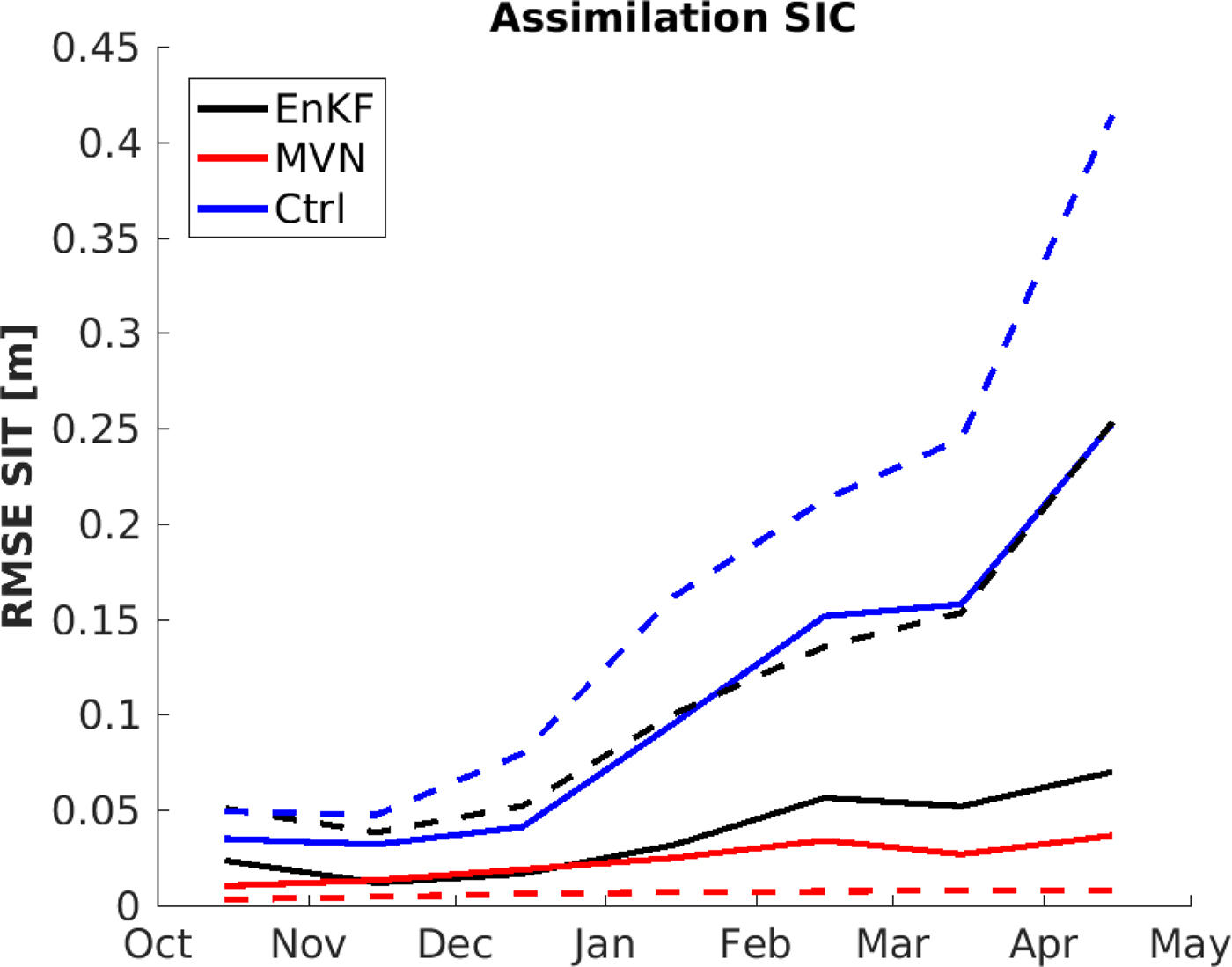
Fig. 5. Monthly mean of RMSE of SIT with and without SIC assimilation. Blue lines are control runs without assimilation, while red and black lines are EnKF- and MVN-assimilated runs, respectively. For the SIT RMSE calculations, only grid points in the marginal ice zone were used, defined as ice concentration <0.8 based on EnKF (solid line) and on MVN (dashed line). The SIT RMSE values were based on 3 years of assimilation.
The SIT RMSE of the EnKF results calculated for the marginal ice zone defined by the MVN model system are significantly higher than the MVN SIT RMSE values. These high SIT RMSE values are caused by an error in the ensemble spread, due to model bias: For the EnKF, the model bias leads to a skewed ensemble spread towards larger ice extent which causes low ensemble spread in the observed marginal ice zone. The marginal ice zone defined by the EnKF assimilation system is then displaced from the observed marginal ice zone. For the MVN assimilation, the one model realization is pushed towards the observations, independent of the model bias. Thus the MVN method has a large effect in the marginal ice zone defined by the observations.
A check for statistical significance of the assimilation skills in Fig. 5 was conducted using a student's t-test with a zero hypothesis of equal values. The result shows that all lines are statistically different on a 95% level, showing that both assimilation methods are better than the control run, and the MVN assimilation shows better skills than does the EnKF assimilation.
A second model experiment was performed where the same method as described above was used, but where SIT was assimilated and SIC was validated against observations. Only grid points where SIT observations exist were used in the validation. The results are shown in Fig. 6. The results describe a similar situation as for the SIC assimilation in Fig. 5. The MVN and EnKF results with both marginal ice zone definitions are significant improvements of the background model. For the marginal ice zone defined by the MVN assimilation, the MVN method showed better skills than the EnKF, Fig. 6. As for the SIC assimilation shown in Fig. 5, this is related to model bias and the way the two assimilation systems update the model parameters: Due to model bias, the EnKF has low ensemble spread in the observed marginal ice zone, while the MVN has a large effect here. This is because the differences between model and observations are large in the marginal ice zone.
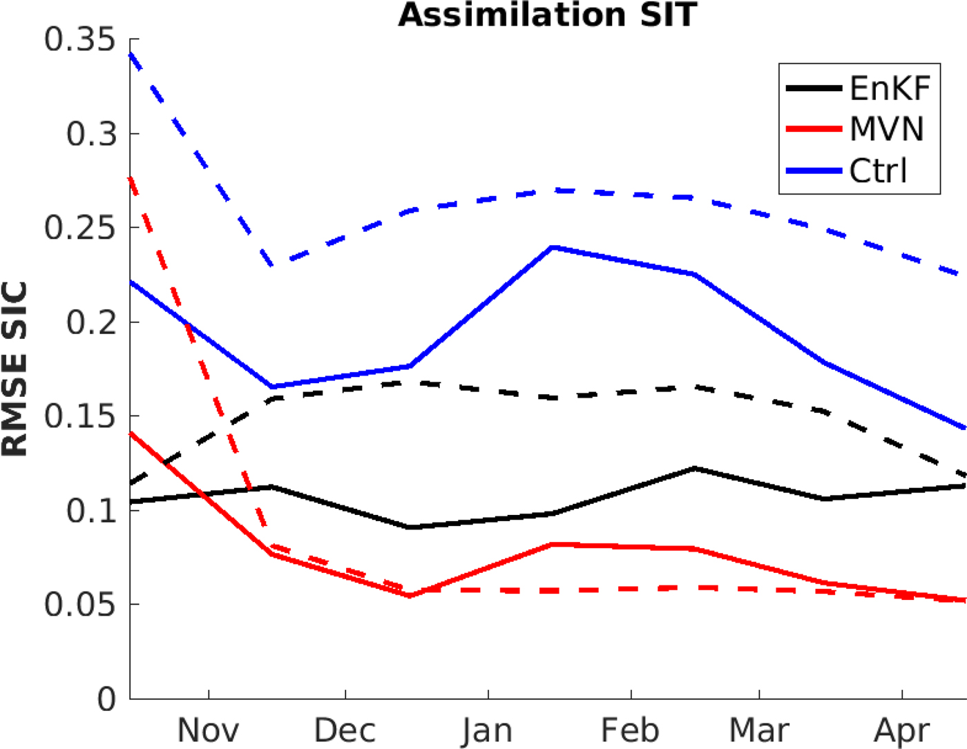
Fig. 6. As Fig. 5, but SIT assimilation and SIC RMSE over two cold seasons.
The difference between the two methods was larger for SIT assimilation (Fig. 6) than for SIC assimilation (5). This is due to few SIT observations available for assimilation, and that the number of observations varies on a daily basis. The daily variations in observation location will lead to an assimilation system which gives comparable results to those of an assimilation system with time steps longer than 10 days. This virtually increased time step is because some locations might only have a local observation every 20 days or more seldom. Since the model has excessive ice during winter, the ice extent will be increased as a consequence of the model bias and variations in observation locations. Increased ice coverage will create an increased biased ensemble spread, and this explains the higher SIC RMSE values for the EnKF compared with the MVN for SIT assimilation. There is no clear temporal tendency for the result in Fig. 6, this is because SIC does not increase as does the SIT (see Fig. 5): SIC is bounded with a maximum value of 1 while SIT is unbounded upwards.
A check for statistical significance of the assimilation skills in Fig. 6 was conducted using a student's t-test with a zero hypothesis of equal values. All lines in Fig. 6 were found to be statistically different on a 95% level, confirming that the MVN method shows better multivariate update than the EnKF and that both methods are an improvement of the control case.
4.1. Spatial correlation
In this section, the spatial properties of the EnKF and MVN were compared by assimilating 25% of all SIC observations. The RMSE values for the SIC in the control model are shown by the blue solid line in Fig. 7. The control model has a large increase of SIC RMSE from April to June, caused by excessive ice growth in the model compared with the observations. In June the ice melting starts and the SIC RMSE of the control model is reduced. In September there is an increase of SIC RMSE due to excessive ice melting which declines in October due to ice growth. Fig. 7 shows that the current model forced by ERA-Interim and ROMS has a too large annual cycle of SIC with excessive ice melting during summer and excessive ice growth during winter. The solid red line in Fig. 7 represents the MVN assimilation where all available SIC observations were used. The MVN assimilation shows large improvements compared with the control model for SIC RMSE values. In summer the MVN assimilation shows a clear weakness with large SIC RMSE values caused by an underestimation of sea-ice extent. During the extended summer period (June–October), a large portion of the ice cover has a SIC <0.8, which in the present study was considered as the marginal ice zone. In the marginal ice zone, the SIT is updated based on the relation given in Eqn (11) for MVN. This relation is based on available winter observations and the applicability in summer is not known, which may be the reason for the large errors in summer. A second reason for the large SIC differences between model and observations in summer is the excessive model ice melting; the assimilated ice is thin and sensitive to the model forcing.
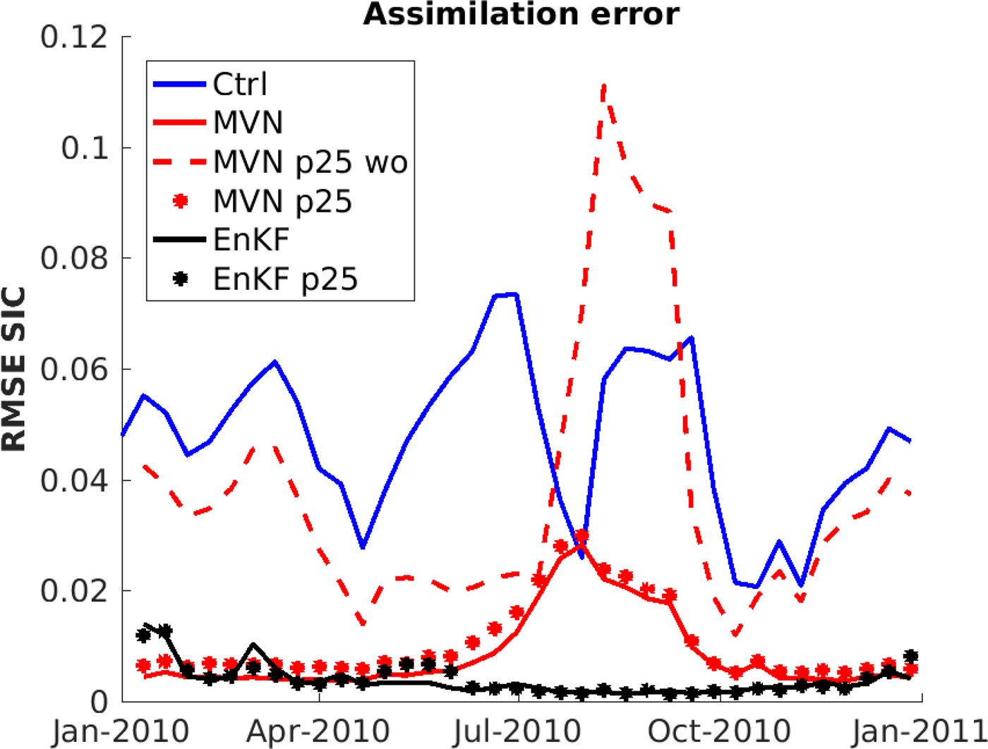
Fig. 7. RMSE of SIC after assimilation of SIC for 2010. For the dotted lines, only25% of the SIC observations were used for the assimilation. The red and black dots are the MVN- and EnKF-assimilated runs, respectively. For the dashed, red line, the MVN assimilation without spatial extrapolation was used for assimilation of 25% of the SIC observations. The solid lines show assimilation using all observations, the blue line is the control model, the red line is the MVN model, and the black line is the EnKF model.
The dashed red line (MVN p25 wo) in Fig. 7 shows the result of MVN assimilation without the extrapolation method when 25% of all SIC observations are assimilated. The SIC RMSE values for this model system are close to those of the control run, dominated by the background forcing. The MVN assimilation without extrapolation, limits the build-up of ice in late spring (April–June). The reduced ice pack in summer leads to an almost ice-free Arctic, due to excessive summer ice melt in the model, which in turn leads to increased SIC RMSE values. This shows that without extrapolation of the observations, the MVN method is not applicable in a situation where the model has large biases, as in this study. The red dots (MVN p25) in Fig. 7 represents the full MVN method with extrapolation when 25% of the observations are used. We found that although the MVN p25 model system has slightly higher SIC RMSE values compared with using all observations, the difference is relatively small.
The black solid line in Fig. 7 represent the EnKF where all observations are used and the black dots (EnKF p25) represent a case using 25% of the SIC observations. The results show small differences between the two cases, indicating that fewer observations are not a problem for the EnKF assimilation. For EnKF there are large initial errors when the assimilation starts, followed by a decrease as the ensemble becomes more heterogeneous around the true state. In summer the EnKF has much lower SIC RMSE values than the MVN, since the EnKF has a large ensemble spread during summer caused by thin ice being more sensitive to the perturbation of the background forcing. The large ensemble spread leads to more weight on the observations during assimilation and low SIC RMSE values. The SIC RMSE values of the EnKF increases slightly in October due to less ensemble spread in the cold season (October–April) as a consequence of thicker ice which requires more energy to melt. This causes biases in the ensemble spread towards larger ice extent as mentioned previously.
A summary of the statistical significance of the results in Fig. 7 is provided in Table 1. The table shows that for MVN there is a statistical difference on a 95% level between the p25 result and the all observations result, all p25 SIC RMSE values are larger than the SIC RMSE values for the all observations case. For EnKF there was no statistical difference between the p25 and the all observations case.
Table 1. Student's t-test to check whether the curves in Fig. 7 are significantly different. Bold values represent statistical difference on a 95% level

5. CONCLUSION
In this study, the EnKF and MVN assimilation methods were used to assimilate SIC and SIT into the state-of-the-art sea-ice model CICE. Compared with the traditional nudging methods, the EnKF has many advantages, for example multivariate update and spatial correlation. The MVN method aims to provide a simple low-cost alternative to the EnKF comparable in quality for sea-ice assimilation. Multivariate update of variables is an important part of the EnKF, where non-observed variables are updated during the assimilation based on correlation with observed variables. This advantageous property of the EnKF has been shown in several earlier works on sea-ice assimilation (Lisæter and others, Reference Lisæter, Rosanova and Evensen2003, Reference Lisæter, Evensen and Laxon2007; Massonnet and others, Reference Massonnet, Fichefet and Goosse2015; Xie and others, Reference Xie, Counillon, Bertino, Tian-Kunze and Kaleschke2016). For the Nudging scheme, the multivariate update of variables is not part of the original method. In the present study, we propose a nudging method with multivariate properties by using a pre-defined relationship between sea-ice volume and SIC as given by Eqns (10) and (11).
In our study, we conducted a cross-validation experiment where SIT or SIC observations were assimilated. The non-assimilated variables were used for validation of the multi-variate properties. We show that multivariate update of sea-ice thickness and concentration is more skilful for MVN than for EnKF. However, the model has biases towards increased sea-ice extent in winter which affect the EnKF ensemble spread.
We show that the spatial properties of the EnKF can to some extent be mimicked by an extrapolation algorithm for the MVN. The extrapolation introduces some extra errors in the assimilation but still lead to a significant improvement as compared with the non-extrapolation method. There are uncertainties regarding the MVN in summer. The relationship between SIC and sea-ice volume for the MVN method is only based on observations from the cold season. In addition, the CICE model in the standalone mode used with ERA/ROMS forcing has excessive ice melting during summer.
The MVN method is not limited to linear correlations as the EnKF. This is an advantage since linear correlation may not be appropriate for bounded values as those of SIC. However, it is important to emphasize the skilful properties of the EnKF for sea-ice assimilation. We show here that the EnKF has excellent out-of-the-box properties when it comes to sea-ice modelling. Without any modifications, the EnKF has similar multivariate skills and better spatial skills than the MVN assimilation. In addition, the EnKF has several useful properties compared with the MVN assimilation. Assimilation of other observations can easily be implemented in the EnKF. The multivariate properties span all variables, not just SIT and SIC, and the relationship between variables change in time and space dependent on the model state. In conclusion, when observations are limited to SIT and SIC, the MVN method performs similarly to the advanced EnKF for sea-ice assimilation. There are still issues regarding the validity of the MVN method in summer, but could likely be solved when summer observations become available.
ACKNOWLEDGMENTS
We thank Geir Evensen and Laurent Bertino at the Nansen center for helpful discussions regarding the Ensemble Kalman filter. We thank Pavel Sakov for help using the EnKF-c and for helpful discussions regarding the EnKF. We also thank Elisabeth Hunke for help with the Los Alamos CICE model and also for the model code. We thank the EUMETSAT OSISAF centre for providing the sea-ice concentration data, and the Integrated Climate Data Center at the University of Hamburg for the SMOS ice thickness observations. This work was funded through the Center for Integrated Remote sensing and Forecast for Arctic Operations through the Norwegian Research Council grant no. 237906. Two supercomputers provided by the Norwegian Metacenter for Computational Science (NOTUR) was used for the computational work, the Vilje computer at the Norwegian University of Science and Technology was used with project NN9348 K and the Stallo computer at the University of Tromsø under project uit-phys-014. We thank the editor and two anonymous reviewers for valuable comments, that helped improve the manuscript. The publication charges for this article have been funded by a grant from the publication fund of UiT The Arctic University of Norway.


 Open access