


1. Introduction
Straight and nearly straight jets have been studied for almost 150 years, since the seminal works of Plateau (Reference Plateau1873) and Rayleigh (Reference Rayleigh1878). Curved jets, on the other hand, have a much shorter history – probably because they cannot be examined using the usual (cylindrical) coordinates. Alternative curvilinear coordinates associated with the jet centreline were suggested by Entov & Yarin (Reference Entov and Yarin1984); even though they are non-orthogonal and, thus, make the Navier–Stokes equations several pages long, they have been successfully applied to gravity-affected slender jets (Wallwork Reference Wallwork2001; Wallwork et al. Reference Wallwork, Decent, King and Schulkes2002; Shikhmurzaev & Sisoev Reference Shikhmurzaev and Sisoev2017; Decent et al. Reference Decent, Părău, Simmons and Uddin2018).
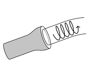
The present paper considers jets where the velocity involves a non-zero swirling component, so that the trajectories of fluid particles are spirals; such jets can be created by inserting a propeller into the orifice. We are concerned with oblique swirling jets: those ejected in a direction other than the vertical, so that their trajectories are curved by gravity. A set of asymptotic equations have been derived for slender jets, i.e. those whose radii of curvature exceed their thickness.
Three highly counter-intuitive results will be presented in this paper.
(i) We show that the Navier–Stokes equations admit asymptotic solutions describing swirling jets which bend upwards, i.e. against gravity. They have yet to be tested for stability, but even if they turn out to be unstable, downward-bending jets are not the alternative, as they do not exist in this range of parameters. The only realistic alternative is unstable, eternally evolving flow.
(Note that solutions describing upward-bending jets have been found before – and not only jets (Wallwork Reference Wallwork2001), but also liquid curtains (Keller & Weitz Reference Keller and Weitz1957; Benilov Reference Benilov2019, Reference Benilov2021). These jets and curtains, however, bend upwards due to surface tension, whereas the jets found in this work do so even if the capillary coefficient is zero. It is the swirling velocity that makes them bend upwards, not surface tension.)
(ii) We show that the streamwise velocity in some downward-bending jets decreases with the distance from the orifice – to the extent that a stagnation point (SP) emerges in the flow. This behaviour is at odds with the intuitive perception that falling objects accelerate due to gravity. It is further argued that SPs cause instability, so that downward jets developing them terminate due to an instability at a finite distance from the orifice.
(Note that the emergence of SPs in swirling flows (not necessarily jets) has been reported before, and is usually referred to as ‘vortex breakdown’ (e.g. Benjamin (Reference Benjamin1962), Escudier (Reference Escudier1988), Brown & Lopez (Reference Brown and Lopez1990), Gelfgat, Bar-Yoseph & Solan (Reference Gelfgat, Bar-Yoseph and Solan1996), Billant, Chomaz & Huerre (Reference Billant, Chomaz and Huerre1998), Ruith et al. (Reference Ruith, Chen, Meiburg and Maxworthy2003), Moise & Mathew (Reference Moise and Mathew2021), Shtern (Reference Shtern2012) and references therein). So far, it has been observed in flows not affected (thus, not accelerated) by gravity, so their slow-down is less counter-intuitive – but it is still the same effect as the one described here. The mere fact that our asymptotic model describes a paradoxical, but known, phenomenon, indirectly validates the rest of our results.)
(iii) Viscosity-dominated jets may reach higher (if they bend upwards) and propagate farther (in all cases) than their inviscid counterparts. The reason is that the latter are prone to be terminated by SPs, whereas the former are affected by cross-stream homogenisation (either eliminating, or at least postponing, formation of SPs).
This paper has the following structure. In § 2, we formulate the problem for an inviscid fluid without surface tension, and in § 3, derive a set of asymptotic equations describing jets with a large Froude number. Examples of solutions of these equations are obtained in § 4, and the results obtained are extended to viscous capillary fluids in § 5. In § 6, we compared our results with those obtained previously for liquid curtains.
2. Formulation of the problem: ideal fluids without surface tension
2.1. Preliminaries
Consider a steady flow of fluid of density  $\rho$ ejected with a flux $F$ from a circular orifice of radius $R_{0}$. Choosing the characteristic velocity scale to be
 \begin{equation} U=\frac{F}{2\left( {\rm \pi}R_{0}^{2}\right) }, \end{equation}
we introduce the reciprocal of the Froude number,
 \begin{equation} \varepsilon =\frac{gR_{0}}{U^{2}}, \end{equation}
where  $g$ is the acceleration due to gravity. It can be shown that the characteristic radius of the jet's curvature due to gravity is
 \begin{equation} L=\frac{R_{0}}{\varepsilon }. \end{equation}
Everywhere in this paper, we assume that  $\varepsilon \ll 1$ – hence, $L\gg R_{0}$ and the slender-jet approximation can be employed.
We shall use the curvilinear coordinates  $( l,r,\phi )$ related to the Cartesian coordinates $( x,y,z)$ by
 \begin{equation} x=\bar{x}+r\sin \alpha \sin \phi ,\quad y={-}r\cos \phi ,\quad z=\bar{z} -r\cos \alpha \sin \phi , \end{equation}
where  $\bar {x}(l)$ and $\bar {y}(l)$ are the coordinates of the jet's centreline, and $\alpha (l)$ is the local angle between the centreline and the horizontal (see figure 1). Observe that the second expression in (2.4a–c) does not include the lateral displacement $\bar {y}(l)$, so that all of the centreline is in the vertical $( x,z)$ plane. It can be readily verified that $( l,r,\phi )$ are orthogonal coordinates (which they would not be, should $\bar {y}(l)$ be introduced in (2.4a–c) (Entov & Yarin Reference Entov and Yarin1984; Shikhmurzaev & Sisoev Reference Shikhmurzaev and Sisoev2017; Decent et al. Reference Decent, Părău, Simmons and Uddin2018)).

Figure 1. The setting: a jet ejected from a circular outlet. Here  $( l,r,\phi )$ are the curvilinear coordinates associated with the jet's centreline, and $\alpha (l)$ is the angle between the centreline and the horizontal.
To identify  $l$ with the centreline's arclength, we require
 $$\begin{gather} \frac{\mathrm{d}\bar{x}}{\mathrm{d}l}=\cos \alpha ,\quad \frac{\mathrm{d} \bar{z}}{\mathrm{d}l}=\sin \alpha , \end{gather}$$
 $$\begin{gather}\bar{x}=0,\quad \bar{z}=0\quad \text{if}\ l=0. \end{gather}$$
Equations (2.5a,b) and boundary conditions (2.6a,b) relate uniquely  $( \bar {x},\bar {z})$ to $\alpha$, whereas the latter remains mathematically undetermined. It will be fixed later as convenient.
2.2. Governing equations
In order to minimise straightforward, yet extremely tedious, algebra associated with the use of curvilinear coordinates, we shall first consider the simplest setting: an ideal fluid without surface tension. Once this limit has been examined, we shall briefly explain how the results can be extended to the general case of viscous capillary jets.
The scaling in the present problem is similar to that used by Benilov (Reference Benilov2019) for liquid curtains. In application to jets, it amounts to introducing the following non-dimensional variables:
 $$\begin{gather} l_{nd}=\frac{l}{L},\quad r_{nd}=\frac{r}{R_{0}},\quad \phi _{nd}=\phi , \end{gather}$$
 $$\begin{gather}\left( u_{l},u_{r},u_{\phi }\right) _{nd}=\frac{\left( u_{l},u_{r},u_{\phi }\right) }{U},\quad p_{nd}=\frac{p}{\rho gL}, \end{gather}$$
where  $( u_{l},u_{r},u_{\phi })$ are the projections of the velocity onto the local axes of the curvilinear coordinates and $p$ is the pressure.
In terms of the non-dimensional variables, the Euler equations have the form (the subscript  $_{nd}$ omitted)
 \begin{align} &\frac{u_{l}}{h_{l}}\frac{\partial u_{l}}{\partial l}+\frac{1}{\varepsilon } \left[ u_{r}\frac{\partial u_{l}}{\partial r}+\frac{u_{\phi }}{r}\frac{ \partial u_{l}}{\partial \phi }+\frac{u_{l}}{h_{l}}\left( u_{r}\frac{ \partial h_{l}}{\partial r}+\frac{u_{\phi }}{r}\frac{\partial h_{l}}{ \partial \phi }\right) \right] +\dfrac{1}{h_{l}}\dfrac{\partial p}{\partial l}\nonumber\\ &\quad ={-}\dfrac{1}{h_{l}}\left( \dfrac{\mathrm{d}z}{\mathrm{d}l}+\varepsilon r\sin \alpha \,\dfrac{\mathrm{d}\alpha }{\mathrm{d}l}\sin \phi \right) , \end{align}
 $$\begin{gather} \dfrac{1}{\varepsilon }\left( \varepsilon \frac{u_{l}}{h_{l}}\frac{\partial u_{r}}{\partial l}+u_{r}\frac{\partial u_{r}}{\partial r}+\frac{u_{\phi }}{r} \frac{\partial u_{r}}{\partial \phi }-\frac{u_{l}^{2}}{h_{l}}\frac{\partial h_{l}}{\partial r}-\frac{u_{\phi }^{2}}{r}+\dfrac{\partial p}{\partial r} \right) =\cos \alpha \sin \phi, \end{gather}$$
 $$\begin{gather}\frac{u_{l}}{h_{l}}\frac{\partial u_{\phi }}{\partial l}+\frac{1}{ \varepsilon }\left( u_{r}\frac{\partial u_{\phi }}{\partial r}+\frac{u_{\phi }}{r}\frac{\partial u_{\phi }}{\partial \phi }+\frac{u_{\phi }u_{r}}{r}- \frac{u_{l}^{2}}{rh_{l}}\frac{\partial h_{l}}{\partial \phi }\right) +\dfrac{ 1}{\varepsilon r}\dfrac{\partial p}{\partial \phi }=\cos \alpha \cos \phi , \end{gather}$$
 $$\begin{gather}\frac{\partial \left( ru_{l}\right) }{\partial l}+\frac{1}{\varepsilon } \left[ \frac{\partial \left( rh_{l}u_{r}\right) }{\partial r}+\frac{\partial \left( h_{l}u_{\phi }\right) }{\partial \phi }\right] =0, \end{gather}$$
where the Lamé coefficient for the variable  $l$ is
 \begin{equation} h_{l}=1+\varepsilon r\frac{\mathrm{d}\alpha }{\mathrm{d}l}\sin \phi . \end{equation}
The other two Lamé coefficients have been replaced with their values,  $h_{r}=1$ and $h_{\phi }=\varepsilon r$.
Let the jet's free boundary be determined by the equation  $r=R(l,\phi )$, where $R$ satisfies the kinematic boundary condition,
 \begin{equation} \dfrac{u_{l}}{h_{l}}\dfrac{\partial R}{\partial l}-\frac{u_{r}}{\varepsilon } +\dfrac{u_{\phi }}{\varepsilon r}\frac{\partial R}{\partial \phi }=0\quad \text{if}\ r=R. \end{equation}
The dynamic boundary condition, in turn, is
 \begin{equation} p=0\quad \text{if}\ r=R. \end{equation}
3. Asymptotic analysis
3.1. Asymptotic equations
Within the framework of the slender-jet approximation, the jet's cross-section is almost circular, and the radial velocity  $u_{r}$ is much smaller than $u_{l}$ and $u_{\phi }$. Thus, we seek a solution of the form
 \begin{equation} \left.\begin{gathered} R =R^{(0)}(l)+\varepsilon R^{(1)}(l,\phi )+O(\varepsilon ^{2}), \\ u_{l} =u_{l}^{(0)}(l,r)+\varepsilon u_{l}^{(1)}(l,r,\phi )+O (\varepsilon ^{2}),\\ u_{r} =0+\varepsilon u_{r}^{(1)}(l,r,\phi )+O(\varepsilon ^{2}),\\ u_{\phi } =u_{\phi }^{(0)}(l,r)+\varepsilon u_{\phi }^{(1)}(l,r,\phi )+ O(\varepsilon ^{2}), \\ p =p^{(0)}(l,r)+\varepsilon p^{(1)}(l,r,\phi )+O(\varepsilon ^{2}). \end{gathered}\right\} \end{equation}
Substituting these expansions into the exact problem (2.9)–(2.15) and keeping the leading order only, we obtain
 $$\begin{gather} -\frac{u_{\phi }^{(0)2}}{r}+\dfrac{\partial p^{(0)}}{\partial r}=0, \end{gather}$$
 $$\begin{gather}p^{(0)}=0\quad \text{if}\ r=R^{(0)}. \end{gather}$$
Evidently, we do not have enough equations to determine the leading-order solution – hence, we have to consider the next order.
The next-to-leading order yields the following equations:
 $$\begin{gather} \frac{u_{\phi}^{(0)}}{r}\frac{\partial u_{l}^{(1)}}{\partial \phi }+\frac{ \partial u_{l}^{(0)}}{\partial r}u_{r}^{(1)}={-}\sin \alpha -\dfrac{\partial p^{(0)}}{\partial l}-u_{l}^{(0)}\frac{\partial u_{l}^{(0)}}{\partial l} -u_{l}^{(0)}u_{\phi }^{(0)}\frac{\mathrm{d}\alpha }{\mathrm{d}l}\cos \phi, \end{gather}$$
 $$\begin{gather}\frac{u_{\phi }^{(0)}}{r}\frac{\partial u_{r}^{(1)}}{\partial \phi }-\frac{ 2u_{\phi }^{(0)}}{r}u_{\phi }^{(1)}+\dfrac{\partial p^{(1)}}{\partial r} =\left( \cos \alpha +u_{l}^{(0)2}\frac{\mathrm{d}\alpha }{\mathrm{d}l} \right) \sin \phi , \end{gather}$$
 $$\begin{gather}\left( \frac{\partial u_{\phi }^{(0)}}{\partial r}+\frac{u_{\phi }^{(0)}}{r} \right) u_{r}^{(1)}+\frac{u_{\phi }^{(0)}}{r}\frac{\partial u_{\phi }^{(1)}}{ \partial \phi }+\dfrac{1}{r}\dfrac{\partial p^{(1)}}{\partial \phi } ={-}u_{l}^{(0)}\frac{\partial u_{\phi }^{(0)}}{\partial l} +\left( \cos \alpha +u_{l}^{(0)2}\frac{\mathrm{d}\alpha }{\mathrm{d}l} \right) \cos \phi , \end{gather}$$
 $$\begin{gather}\frac{\partial \left( ru_{r}^{(1)}\right) }{\partial r}+\frac{\partial u_{\phi }^{(1)}}{\partial \phi }={-}r\frac{\partial u_{l}^{(0)}}{\partial l} -ru_{\phi }^{(0)}\frac{\mathrm{d}\alpha }{\mathrm{d}l}\cos \phi \end{gather}$$
and the following boundary conditions:
 \begin{equation} u_{r}^{(1)}-\dfrac{u_{\phi }^{(0)}}{r}\frac{\partial R^{(1)}}{\partial \phi } =u_{l}^{(0)}\dfrac{\mathrm{d}R^{(0)}}{\mathrm{d}l},\quad p^{(1)}+R^{(1)} \frac{\partial p^{(0)}}{\partial r}=0\quad \text{if}\ r=R^{(0)}. \end{equation}
Boundary-value problem (3.4)–(3.8a,b) is consistent with the following ansatz:
 \begin{equation} \left.\begin{gathered} u_{l}^{(1)}=u_{l}^{(1,0)}(l,r)+u_{l}^{(1,1)}(l,r)\sin \phi ,\quad u_{r}^{(1)}=u_{r}^{(1,0)}(l,r)+u_{r}^{(1,1)}(l,r)\cos \phi ,\\ u_{\phi }^{(1)}=u_{\phi }^{(1,0)}(l,r)+u_{\phi }^{(1,1)}(l,r)\sin \phi, \quad p^{(1)}=p^{(1,0)}(l,r)+p^{(1,1)}(l,r)\sin \phi ,\\ R^{(1)}=R^{(1,0)}(l)+R^{(1,1)}(l)\sin \phi , \end{gathered}\right\} \end{equation}
where the functions with the superscripts  $^{(1,0)}$ and $^{(1,1)}$ satisfy two non-coupled problems,
 $$\begin{gather} \frac{\partial u_{l}^{(0)}}{\partial r}u_{r}^{(1,0)}={-}\sin \alpha -\dfrac{ \partial p^{(0)}}{\partial l}-u_{l}^{(0)}\frac{\partial u_{l}^{(0)}}{ \partial l}, \end{gather}$$
 $$\begin{gather}-\frac{2u_{\phi }^{(0)}}{r}u_{\phi }^{(1,0)}+\dfrac{\partial p^{(1,0)}}{ \partial r}=0, \end{gather}$$
 $$\begin{gather}\left( \frac{\partial u_{\phi }^{(0)}}{\partial r}+\frac{u_{\phi }^{(0)}}{r} \right) u_{r}^{(1,0)}={-}u_{l}^{(0)}\frac{\partial u_{\phi }^{(0)}}{\partial l} , \end{gather}$$
 $$\begin{gather}\frac{\partial \left( ru_{r}^{(1,0)}\right) }{\partial r}={-}r\frac{\partial u_{l}^{(0)}}{\partial l}, \end{gather}$$
 $$\begin{gather}u_{r}^{(1,0)}=u_{l}^{(0)}\dfrac{\mathrm{d}R^{(0)}}{\mathrm{d}l}\quad \text{if}\ r=R^{(0)}, \end{gather}$$
 $$\begin{gather}p^{(1,0)}+R^{(1,0)}\frac{\partial p^{(0)}}{\partial r}=0\quad \text{if} \ r=R^{(0)} \end{gather}$$
and
 $$\begin{gather} \frac{u_{\phi }^{(0)}}{r}u_{l}^{(1,1)}+\frac{\partial u_{l}^{(0)}}{\partial r }u_{r}^{(1,1)}={-}u_{l}^{(0)}u_{\phi }^{(0)}\frac{\mathrm{d}\alpha }{\mathrm{d} l}, \end{gather}$$
 $$\begin{gather}-\frac{u_{\phi }^{(0)}}{r}u_{r}^{(1,1)}-\frac{2u_{\phi }^{(0)}}{r}u_{\phi }^{(1,1)}+\dfrac{\partial p^{(1,1)}}{\partial r}=\cos \alpha +u_{l}^{(0)2} \frac{\mathrm{d}\alpha }{\mathrm{d}l}, \end{gather}$$
 $$\begin{gather}\left( \frac{\partial u_{\phi }^{(0)}}{\partial r}+\frac{u_{\phi }^{(0)}}{r} \right) u_{r}^{(1,1)}+\frac{u_{\phi }^{(0)}}{r}u_{\phi }^{(1,1)}+\dfrac{1}{r} p^{(1,1)}=\cos \alpha +u_{l}^{(0)2}\frac{\mathrm{d}\alpha }{\mathrm{d}l}, \end{gather}$$
 $$\begin{gather}\frac{\partial \left( ru_{r}^{(1,1)}\right) }{\partial r}+u_{\phi }^{(1,1)}={-}ru_{\phi }^{(0)}\frac{\mathrm{d}\alpha }{\mathrm{d}l}, \end{gather}$$
 $$\begin{gather}u_{r}^{(1,1)}-\dfrac{u_{\phi }^{(0)}}{r}R^{(1,1)}=0\quad \text{if}\ r=R^{(0)}, \end{gather}$$
 $$\begin{gather}p^{(1,1)}+R^{(1,1)}\frac{\partial p^{(0)}}{\partial r}=0\quad \text{if} \ r=R^{(0)}. \end{gather}$$
Expressing  $u_{r}^{(1,0)}$ from (3.10) and substituting it into (3.12)–(3.14), we obtain
 $$\begin{gather} \left( \dfrac{\partial u_{\phi }^{(0)}}{\partial r}+\dfrac{u_{\phi }^{(0)}}{r }\right) \left( u_{l}^{(0)}\frac{\partial u_{l}^{(0)}}{\partial l}+\dfrac{ \partial p^{(0)}}{\partial l}+\sin \alpha \right) =u_{l}^{(0)}\frac{\partial u_{\phi }^{(0)}}{\partial l}\dfrac{\partial u_{l}^{(0)}}{\partial r}, \end{gather}$$
 $$\begin{gather}\frac{\partial }{\partial r}\left[ \frac{r}{\dfrac{\partial u_{l}^{(0)}}{ \partial r}}\left( u_{l}^{(0)}\frac{\partial u_{l}^{(0)}}{\partial l}+\dfrac{ \partial p^{(0)}}{\partial l}+\sin \alpha \right) \right] =r\frac{\partial u_{l}^{(0)}}{\partial l}, \end{gather}$$
 $$\begin{gather}\frac{1}{\dfrac{\partial u_{l}^{(0)}}{\partial r}}\left( u_{l}^{(0)}\frac{ \partial u_{l}^{(0)}}{\partial l}+\dfrac{\partial p^{(0)}}{\partial l}+\sin \alpha \right) \rightarrow -u_{l}^{(0)}\dfrac{\mathrm{d}R^{(0)}}{\mathrm{d}l} \quad \text{as}\ r\rightarrow R^{(0)}. \end{gather}$$
Observe that (3.22)–(3.24) include only the leading-order unknowns and, thus, can be viewed as the solvability conditions for boundary-value problem (3.10)–(3.15).
To derive the solvability condition(s) for problem (3.16)–(3.21), one should express  $u_{\phi }^{(1,1)}$ from (3.19), and substitute it into (3.18) and (3.17) – which yield, after straightforward algebra,
 $$\begin{gather} \frac{\partial }{\partial r}\left[ ru_{\phi }^{(0)2}\frac{\partial }{ \partial r}\left( \frac{ru_{r}^{(1,1)}}{u_{\phi }^{(0)}}\right) \right] ={-} \frac{\mathrm{d}\alpha }{\mathrm{d}l}\left[ 2r^{2}\left( u_{l}^{(0)}\frac{ \partial u_{l}^{(0)}}{\partial r}+u_{\phi }^{(0)}\frac{\partial u_{\phi }^{(0)}}{\partial r}\right) +3ru_{\phi }^{(0)2}\right] , \end{gather}$$
 $$\begin{gather}p^{(1,1)}=ru_{\phi }^{(0)}\frac{\partial u_{r}^{(1,1)}}{\partial r}-r\frac{ \partial u_{\phi }^{(0)}}{\partial r}u_{r}^{(1,1)}+r\cos \alpha +r\left( u_{l}^{(0)2}+u_{\phi }^{(0)2}\right) \frac{\mathrm{d}\alpha }{\mathrm{d}l}. \end{gather}$$
Substituting the above expression for  $p^{(1,1)}$ into condition (3.21) and recalling (3.20), we obtain
 \begin{equation} u_{\phi }^{(0)2}\frac{\partial }{\partial r}\left( \frac{ru_{r}^{(1,1)}}{ u_{\phi }^{(0)}}\right) ={-}r\cos \alpha -r\left( u_{l}^{(0)2}+u_{\phi }^{(0)2}\right) \frac{\mathrm{d}\alpha }{\mathrm{d}l}\quad \text{if}\ r=R^{(0)}. \end{equation}
Integrating (3.25) from  $r=0$ to $r=R^{(0)}$ and taking into account condition (3.27), we observe that a solution for $u_{r}^{(1,1)}$ exists only if
 \begin{equation} -R^{(0)2}\cos \alpha =\frac{\mathrm{d}\alpha }{\mathrm{d}l} \int_{0}^{R^{(0)}}r\left( 2u_{l}^{(0)2}-u_{\phi }^{(0)2}\right) \mathrm{d}r. \end{equation}
Given suitable entry conditions at the orifice, (3.2), (3.22)–(3.23), (3.28) and boundary conditions (3.3), (3.24) fully determine  $u_{l}^{(0)}(l,r)$, $u_{\phi }^{(0)}(l,r)$, $p^{(0)}(l,r)$ and $\alpha (l)$. Once these are found, one can use (2.5a,b)–(2.6a,b), to find $\bar {x}(l)$ and $\bar {z}(l)$ – i.e. the jet's trajectory.
3.2. Discussion: singular points of the equations derived
Observe that (3.23) and boundary condition (3.24) appear to be singular if/where  $\partial u_{l}^{(0)}/\partial r=0$. It turns out, however, that the apparent singularity of the boundary-value problem does not translate into singularity of the solution.
To understand why, integrate (3.23) from  $r=0$ to $r=R^{(0)}$, take into account (3.24) and thus obtain
 \begin{equation} \dfrac{\mathrm{d}}{\mathrm{d}l}\int_{0}^{R^{(0)}}ru_{l}^{(0)}\,\mathrm{d}r=0. \end{equation}
Integrating this equation with respect to  $l$ and equating (without loss of generality) the constant of integration to unity, we obtain
 \begin{equation} \int_{0}^{R^{(0)}}ru_{l}^{(0)}\,\mathrm{d}r=1. \end{equation}
This (non-singular) equality reflects conservation of the mass flux. In what follows, it will replace the singular condition (3.24).
To resolve the singularity in (3.23), we note that the asymptotic boundary-value problem is invariant with respect to simultaneously changing
 \begin{equation} \left( l,r\right) \rightarrow \left( l,-r\right) ,\quad ( u_{l}^{(0)},u_{\phi }^{(0)},p^{(0)}) \rightarrow ( u_{l}^{(0)},-u_{\phi }^{(0)},p^{(0)}) . \end{equation}
Thus,  $u_{l}^{(0)}$ and $p^{(0)}$ can be analytically extended to the region $r<0$ as even functions, whereas $u_{\phi }^{(0)}$ can be extended as an odd function. Since all three should be analytic at $r=0$, this implies
 \begin{equation} \frac{\partial u_{l}^{(0)}}{\partial r}=O(r),\quad \frac{\partial p^{(0)}}{\partial r}=O(r),\quad u_{\phi }^{(0)}=O (r)\quad \text{as}\ r\rightarrow 0. \end{equation}
Then, as follows from (3.22),
 \begin{equation} u_{l}^{(0)}\frac{\partial u_{l}^{(0)}}{\partial l}+\dfrac{\partial p^{(0)}}{ \partial l}+\sin \alpha =O(r^{2})\quad \text{as}\ r\rightarrow 0. \end{equation}
Keeping this in mind, we integrate (3.23) from  $r=0$ to $r=r^{\prime }$, interchange $r\leftrightarrow r^{\prime }$, and obtain
 \begin{equation} u_{l}^{(0)}\frac{\partial u_{l}^{(0)}}{\partial l}+\dfrac{\partial p^{(0)}}{ \partial l}+\sin \alpha =\frac{1}{r}\dfrac{\partial u_{l}^{(0)}}{\partial r} \int_{0}^{r}r^{\prime }\frac{\partial u_{l}^{(0)}(l,r^{\prime })}{\partial l} \mathrm{d}r^{\prime }, \end{equation}
where functions without explicitly stated arguments depend on  $( l,r)$. Using (3.34), we reduce (3.22) to
 \begin{equation} \left(\dfrac{\partial u_{\phi }^{(0)}}{\partial r}+\dfrac{u_{\phi }^{(0)}}{r }\right) \frac{1}{r}\int_{0}^{r}r^{\prime }\frac{\partial u_{l}^{(0)}(l,r^{\prime })}{\partial l}\mathrm{d}r^{\prime }=u_{l}^{(0)} \frac{\partial u_{\phi }^{(0)}}{\partial l}. \end{equation}
4. Inviscid jets
To simplify the notation, we change
 \begin{equation} u_{l}^{(0)}\rightarrow u,\qquad u_{\phi }^{(0)}\rightarrow w,\qquad R^{(0)}\rightarrow R. \end{equation}
Now, (3.2), (3.28)–(3.35) and boundary condition (3.28) become
 $$\begin{gather} u\frac{\partial u}{\partial l}+\dfrac{\partial p}{\partial l}+\sin \alpha = \frac{1}{r}\dfrac{\partial u}{\partial r}\int_{0}^{r}r^{\prime }\frac{ \partial u(l,r^{\prime })}{\partial l}\mathrm{d}r^{\prime }, \end{gather}$$
 $$\begin{gather}u\frac{\partial w}{\partial l}=\frac{1}{r}\left( \dfrac{\partial w}{\partial r}+\dfrac{w}{r}\right) \int_{0}^{r}r^{\prime }\frac{\partial u(l,r^{\prime }) }{\partial l}\mathrm{d}r^{\prime }, \end{gather}$$
 $$\begin{gather}-\frac{w^{2}}{r}+\dfrac{\partial p}{\partial r}=0, \end{gather}$$
 $$\begin{gather}\frac{\mathrm{d}\alpha }{\mathrm{d}l}\int_{0}^{R}r\left( w^{2}-2u^{2}\right) \mathrm{d}r=R^{2}\cos \alpha , \end{gather}$$
 $$\begin{gather}\int_{0}^{R}ru\,\mathrm{d}r=1, \end{gather}$$
 $$\begin{gather}p=0\quad \text{if}\ r=R. \end{gather}$$
The solution should be analytic at  $r=0$, which implies
 \begin{equation} \frac{\partial u}{\partial r}=0,\quad w=0\quad \text{if}\ r=0. \end{equation}
It can be shown that, on the  $( l,r)$ plane, boundary-value problem (4.2)–(4.7) is hyperbolic and, as such, requires entry conditions at the orifice. We assume that
 \begin{gather} R=1,\quad u=u_{0}(r),\quad w=w_{0}(r)\quad \text{at}\ l=0, \end{gather}
 \begin{gather} \alpha =\alpha _{0}\quad \text{at}\ l=0, \end{gather}
where the jet's initial radius matches that of the orifice, and  $[u_{0}(r),w_{0}(r)]$ and $\alpha _{0}$ are the ejection velocity and angle, respectively. Note that $u_{0}(r)$ should comply with (4.6), i.e.
 \begin{equation} \int_{0}^{1}ru_{0}\,\mathrm{d}r=1. \end{equation}
This requirement is not a restriction, as it can be always enforced via a proper choice of the scale  $U$ during non-dimensionalisation.
Note also that, near the orifice, the jet may experience certain adjustments – e.g. slight reduction of its radius. These adjustments are not described by the slender-jet approximation, but they can be still accounted for by changing entry conditions (4.9a–c)–(4.10). In this case, the point  $l=0$ would correspond to a cross-section located at a certain distance from the actual orifice.
Finally, changing  $\bar {x}\rightarrow x$ and $\bar {z}\rightarrow z$, we write (2.5a,b)–(2.6a,b) in the form
 $$\begin{gather} \frac{\mathrm{d}\kern0.06em x}{\mathrm{d}l}=\cos \alpha ,\quad \frac{\mathrm{d}z}{ \mathrm{d}l}=\sin \alpha , \end{gather}$$
 $$\begin{gather}x=0,\quad z=0\quad \text{if}\ l=0. \end{gather}$$
4.1. Exact results
Some of the mathematical properties of boundary-value problem (4.2)–(4.13a,b) have far-reaching physical consequences.
(i) If
(4.14)(4.5) implies that \begin{equation} \int_{0}^{1}r( w^{2}-2u^{2}) \mathrm{d}r>0, \end{equation}$\mathrm {d}\alpha /\mathrm {d}l>0$.
Thus, if the swirling velocity
$w$ is sufficiently large, the jet bends upwards, against gravity.To understand the physics behind such a counter-intuitive behaviour, we rewrite (4.5) as a balance of the centrifugal force and gravity,
(4.15)The right-hand side of this equality represents the cross-stream component of the gravitational force acting on a cross-section of radius\begin{equation} \frac{1}{2}\frac{\mathrm{d}\alpha }{\mathrm{d}l}\left( 2{\rm \pi} \int_{0}^{R}rw^{2}\,\mathrm{d}r\right) -\frac{\mathrm{d}\alpha }{\mathrm{d}l} \left( 2{\rm \pi} \int_{0}^{R}ru^{2}\,\mathrm{d}r\right) ={\rm \pi} R^{2}\cos \alpha . \end{equation}$R$ – and the first/second term on the left-hand side describes the contribution of the swirl/streamwise velocity to the centrifugal force. To understand the structure of the latter is easy: one should only keep in mind that $\mathrm {d }\alpha /\mathrm {d}l$ is the curvature of the jet's centreline, and the minus in front shows that the centrifugal force is directed away from the centre of curvature.
As for the swirl contribution to the centrifugal force, it is also proportional to
$\mathrm {d}\alpha /\mathrm {d}l$ (because the forces affecting individual particles in a straight swirling jet average out to zero). Most importantly, this term's sign is opposite to that of its streamwise counterpart.To understand why, consider, say, an upward-bending jet. It is clear from basic geometry that its upper half slightly shrinks, whereas the lower half expands – hence, the trajectories of particles swirling through the former are curved more than those in the latter. Due to this difference and the fact that the centrifugal force is proportional to the curvature of the particles’ trajectories, the swirl part of the force affecting the whole cross-section is directed upwards, i.e. opposite to the streamwise part.
Thus, the upward bending of a swirling jet could be understood through an analogy with a system of two interconnected bodies: one with positive mass and another, with negative. If the absolute value of the latter exceeds that of the former, gravity makes the whole system soar.
(ii) Given the counter-intuitive nature of property (i), it should be reassuring to ascertain that our equations are consistent with basic physical principles. Two of these are discussed below.
(a) Boundary-value problem (4.2)–(4.13a,b) is consistent with the following ansatz:
(4.16a–c)where\begin{equation} u(l,r)=u(l),\quad w(l,r)=0,\quad p(l,r)=0, \end{equation}$u(l)$, $\alpha (l)$ and $R(l)$ satisfy
(4.17a–c)Using (4.12a,b)–(4.13a,b), one can show that the above equations describe free-falling liquid, such that the particles follow parabolic trajectories.\begin{equation} uR=2,\quad u\frac{\mathrm{d}u}{\mathrm{d}l}+\sin \alpha =0,\quad - \frac{ \mathrm{d}\alpha }{\mathrm{d}l}u^{2}=R\cos \alpha . \end{equation}(b) It follows from (4.2)–(4.13a,b) that
(4.18)which reflects conservation of the energy flux through the jet's cross-section. This property of the asymptotic model is helpful for controlling the accuracy of numerical simulations.\begin{equation} \frac{\mathrm{d}}{\mathrm{d}l}\int_{0}^{R}\left( \frac{u^{2}+w^{2}}{2} +p+z\right) ur\,\mathrm{d}r=0, \end{equation}One can also show that
(4.19)These ‘local’ conservation laws do not seem to have physical meaning, but one of them happens to be useful anyway.\begin{equation} \left.\begin{gathered} \frac{\mathrm{d}}{\mathrm{d}l}\left[ \left( \frac{u^{2}}{2}+p\right) _{r=0}+z\right] =0,\\ \frac{\mathrm{d}}{\mathrm{d}l}\left[ \left( \frac{1}{u}\frac{\partial w}{ \partial r}\right) _{r=0}\right] =0. \end{gathered}\right\} \end{equation}
(iii) Important information can be obtained by relating
$\partial u/\partial l$, $\partial w/\partial l$ and $\mathrm {d}R/\mathrm {d}l$ to $u$, $w$ and $R$ (in (4.2)–(4.13a,b), the former are related to the latter implicitly).Differentiating (4.4) with respect to
$l$ and using the resulting equation and (4.2) to eliminate $\partial w/\partial l$ and $\partial p/\partial l$ from (4.3), one obtains
(4.20)where\begin{equation} \frac{\partial }{\partial r}\left( \frac{1}{r}\frac{\partial v}{\partial r} \right) +\frac{1}{u}\left[ \frac{2w}{r^{2}u}\left( \frac{\partial w}{ \partial r}+\frac{w}{r}\right) -\dfrac{\partial }{\partial r}\left( \frac{1}{ r}\dfrac{\partial u}{\partial r}\right) \right] v=0, \end{equation}(4.21)Next, one can use boundary conditions (4.6)–(4.8a,b) to verify that\begin{equation} v(l,r)=\int_{0}^{r}r^{\prime }\frac{\partial u(l,r^{\prime })}{\partial l} \,\mathrm{d}r^{\prime }. \end{equation}(4.22)$$\begin{gather} \frac{\partial }{\partial r}\left( \frac{1}{r}\frac{\partial v}{\partial r} \right) \rightarrow 0\quad \text{as}\ r\rightarrow 0, \end{gather}$$(4.23)Given$$\begin{gather}\frac{\partial v}{\partial r}+\frac{1}{u}\left( \frac{w^{2}}{Ru}-\dfrac{ \partial u}{\partial r}\right) v+\frac{R}{u}\sin \alpha =0\quad \text{if} \ r=R. \end{gather}$$$u$, $w$ and $R$, boundary-value problem (4.20), (4.22)–(4.23) determines $v$, and then (4.21) yields
(4.24)Observe that, if a pair\begin{equation} \frac{\partial u}{\partial l}=\frac{1}{r}\frac{\partial v}{\partial r}. \end{equation}$( l,r)$ exist such that $u(l,r)=0$ the coefficients in (4.20) become singular. In what follows, such pairs will be called SPs even if $w(l,r)\neq 0$.(iv) It follows from (4.20) that
$\partial u/\partial l$ is singular at SPs (see Appendix A.1). The following physical aspects of these singularities are worth noting.


(a) Given the hyperbolic nature of our equations and the fact that the streamlines are their characteristics, it comes as no surprise that the solution becomes singular where one of the characteristics ‘stops’.
(b) If viscosity is introduced, the solution becomes regular (due to the fact that the governing equations become parabolic, see § 6 below).
(c) The presence of an SP invalidates – at least, locally – the assumption that the Froude number be large (which underlies all of our results). Whether this invalidates the global solution is unclear – but is also unimportant in view of item (d), below.
(d) Stagnation points in ideal fluids often make the flow unstable (Friedlander & Vishik Reference Friedlander and Vishik1991), and even in viscous fluids they are a destabilising influence (Benilov & Lapin Reference Benilov and Lapin2014). It is safe to assume that an inviscid or weakly viscous jet exists only between the orifice and the first SP, and it breaks up immediately after it.
4.2. Numerical results
Boundary-value problem (4.2)–(4.13a,b) was solved numerically using the method of lines (Schiesser Reference Schiesser1978): the  $r$ axis was discretised, so that the governing (partial differential) equations turned into a large set of ordinary-differential equations. These equations are implicit with respect to the $l$-derivatives, which were solved for (at each step in $l$) using the MATLAB function FSOLVE. The actual integration of the equations was carried out using the function ODE15s (an adaptive-step solver designed for stiff problems). For reasons explained above, the solutions were terminated at the first SP (if any).
Several particular cases of entry conditions where simulated, but the results will be presented only for the simplest one,
 \begin{equation} u_{0}=2,\quad w_{0}=\omega _{0}r, \end{equation}
where the value of  $u_{0}$ was chosen to satisfy constraint (4.11). If there were no gravity, conditions (4.25a,b) would describe a non-sheared solid-body-rotating flow (as seen later, this is convenient when comparing inviscid and viscous jets). According to condition (4.14), upward-bending jets exist if and only if
 \begin{equation} \omega _{0}>4. \end{equation}
Figure 2 shows the trajectories of four jets with the same ejection angle, but different  $\omega _{0}$. The following features can be observed.

Figure 2. The trajectories of inviscid jets described by boundary-value problem (4.2)–(4.13a,b), with entry conditions (4.24) and  $\alpha _{0}=0$. The curves are marked with corresponding values of $\omega _{0}$. Note that curve (1) is the only one that continues indefinitely, whereas curve (5) continues beyond the boundary of this figure, but eventually stops.
(i) As expected, the two jets satisfying condition (4.26) bend upwards.
(ii) Out of the four jets depicted, three are terminated by SPs
(a) In the downward-bending jet with
$\omega _{0}=3$ and upward-bending jet with $\omega _{0}=7$, the SPs emerge on the jet's axis (see figures 3b and 4b).
Figure 3. The cross-sectional profiles of the streamwise velocity
$u$ and swirl velocity $w$ for the (upward-bending) jets with (a,b) $\omega _{0}=5$ and (c,d) $\omega _{0}=7$. The positions of the cross-sections are marked on the jets’ trajectories in figure 2 by circles with the corresponding values of $\omega _{0}$.(b) In the upward-bending jet with
$\omega _{0}=5$, the SP emerges somewhere between the axis and free surface (unfortunately, we have been unable to finish this computation due to numerical instability, so figure 3(a) shows only the tendency of developing an SP).
(iii) Not all downward-bending jets develop SPs, as illustrated in figure 4(a) for the jet with
$\omega _{0}=1$. The fluid particles in this case do accelerate on the way down.


Figure 4. The cross-sectional profiles of the streamwise velocity  $u$ and swirl velocity $w$ for the (downward-bending) jets with (a,b) $\omega _{0}=1$ and (c,d) $\omega _{0}=3$. The positions of the cross-sections are marked on the jets’ trajectories in figure 2 by circles with the corresponding values of $\omega _{0}$.
Figure 5 illustrates how the behaviour of jets depends on the ejection angle – with the conclusion that  $\alpha _{0}$ affects the trajectory only near the orifice, but the rest of the behaviour is determined by $\omega _{0}$. However, there is a counter-intuitive feature in this case too, as illustrated in figure 6. The jet depicted in this figure is one of those that should bend downwards and develop an SP – but the ejection angle is positive – so, initially, the jet is rising. Given this, its streamwise velocity should be decreasing everywhere in the jet's cross-section, but figure 6 shows that the velocity on the jet's axis initially grows and reaches its maximum at the top of the trajectory. After that, the jet switches to the behaviour expected for this value of $\omega _{0}$ and maintains it until it is terminated by an SP.

Figure 5. The trajectories of jets with  $\omega _{0}=3.5$ and various $\alpha _{0}$. The curves are marked by the corresponding values of $\alpha _{0}$ (in degrees).

Figure 6. The cross-sectional velocity profiles for the (downward-bending) jet with  $\omega _{0}=3.5$ and $\alpha _{0}=45^{\circ }$. One can see that fluid particles on the jet's axis accelerate on the way up and decelerate on the way down.
We simulated numerous other entry conditions, and the following tendencies were observed.
(i) If condition (4.14) holds at the orifice, it continues to hold for the rest of the trajectory. Thus, if a jet bends upwards near the orifice, it bends upwards everywhere.
(ii) Upward-bending jets typically develop SPs (either on or off the axis). In some cases, however, it is impossible to actually see the SP, as our numerical method becomes unstable due to the emergence of a region with highly sheared
$w$. (Refining the mesh did not help in this case, suggesting that the root cause of the instability is a physical one, e.g. a tangential jump emerging in the cross-stream profile of $w$. Unfortunately, we have been unable to verify this hypothesis beyond reasonable doubt, as this would require a completely different numerical method: one suitable for weak solutions. Furthermore, even if tangential jumps do occur in reality, they are closely followed by emergence of an SP which breaks the jet up anyway.)(iii) Downward-bending jets with
$\alpha _{0}<0$ develop SPs only at $r=0$, and only if
(4.27)i.e. at the centre of the orifice, particles decelerate in the streamwise direction.\begin{equation} \frac{\partial u}{\partial l}<0\quad \text{at}\ l=0,\ r=0, \end{equation}


Conclusion (iii) allows one to use boundary-value problem (4.20), (4.22)–(4.23) to derive a sufficient criterion for detecting SPs in downward bending jets. For entry conditions (4.25a,b) and  $\alpha _{0}<0$, criterion (4.27) amounts to (see Appendix A.2)
 \begin{equation} 4\,\textrm{J}_{0}\left( \omega _{0}\right) +\omega _{0}\textrm{J}_{1}\left( \omega _{0}\right) <0, \end{equation}
where  $\textrm {J}_{n}(\omega _{0})$ is the Bessel function of the first kind. Keeping in mind that jets with entry conditions (4.25a,b) bend downwards only if $\omega _{0}<4$, one can show that (4.28) yields
 \begin{equation} 2.9892\lesssim \omega _{0}<4. \end{equation}
This condition agrees with our numerical results very well; and not only for negative  $\alpha _{0}$, but also for most positive ones (in which case criterion (4.28) is formally inapplicable). This is probably due to the fact that, for a downward-bending jet, an initially positive $\alpha$ rapidly becomes negative, so that $u$ and $w$ remain close to their entry profiles.
4.3. Approximate results: near-critical jets
Our asymptotic model (4.2)–(4.13a,b) was derived under the sole assumption that the Froude number is large, but the derived equations are not simple enough to be solved analytically. Thus, it is worthwhile to try to find some extra assumptions allowing one to further simplify (4.2)–(4.13a,b). To avoid confusion, the results of such analyses will be called ‘approximate’, with the word ‘asymptotic’ reserved for boundary-value problem (4.2)–(4.13a,b) itself.
Denote
 \begin{equation} \delta =\int_{0}^{1}r( w_{0}^{2}-2u_{0}^{2}) \mathrm{d}r, \end{equation}
and consider a near-critical regime, i.e. such that
 \begin{equation} \left\vert \delta \right\vert \ll 1. \end{equation}
Under this assumption, all parameters of the jet can be calculated approximately.
Admittedly, the extra assumption can make our asymptotic model inconsistent due to the fact that some of the retained terms can now be smaller than the omitted ones. Since the latter are  $O(\varepsilon )$, one can ensure consistency by requiring $\vert \delta \vert \ll \varepsilon$. This constraint could be replaced with a weaker one, $\vert \delta \vert \lesssim \varepsilon$, if the near-critical regime were examined using the exact Navier–Stokes equations (which is, however, beyond the scope of the present work).
Numerical experiments show that near-critical jets evolve in two stages. First, only  $\alpha$ varies with $l$, whereas $u$,
$u$,  $w$,
$w$,  $p$ and $R$ remain virtually unchanged – i.e. the jet's trajectory is curved, but all other characteristics are close to their entry values. Second, $\alpha$ approaches either ${\rm \pi} /2$ or $-{\rm \pi} /2$, after which the rest of the characteristics start to evolve.
The second stage is difficult to examine analytically, but the first stage, is easy (see Appendix B). The approximate results have been compared with the numerical solution of asymptotic problem (4.2)–(4.13a,b) for entry conditions (4.25a,b), see in figure 7. One can see that the approximate solution predicts the shape of the trajectory well even if  $\delta =1$.


Note that the approximate results assume that  $u$ is close to its entry value: hence, they are not applicable near the SP. However, if $\delta$ is indeed small, the approximate solution does predict the position of the stagnation (termination) point reasonably well (see figure 7).
5. Viscous capillary fluids
5.1. The asymptotic equations
It is well known that the behaviour and characteristics of an inviscid flow can be qualitatively different from those of a viscous one. Thus, it is essential to verify whether upward-bending jets and jets with SPs can be observed in the presence of viscosity.
Let the fluid's kinematic viscosity and surface tension be  $\nu$ and $\sigma$, respectively. Then, in addition to the Froude number, two extra non-dimensional parameters arise: the so-called ‘reduced Reynolds number’ and the Weber number. We shall use their reciprocals, namely,
 \begin{equation} \mu =\frac{\nu L}{UR_{0}^{2}},\quad \gamma =\frac{\sigma }{\rho R_{0}U^{2}}, \end{equation}
where  $L$ is defined by (2.3). Omitting the details (which are similar to those of the inviscid non-capillary case (see Dubovskaya Reference Dubovskaya2020)), we only formulate the resulting asymptotic equations.
To incorporate viscosity and surface tension in set (4.2)–(4.13a,b), one needs to replace (4.2)–(4.3), (4.5) and boundary condition (4.7) with
 $$\begin{gather} u\frac{\partial u}{\partial l}+\dfrac{\partial p}{\partial l}+\sin \alpha = \frac{1}{r}\dfrac{\partial u}{\partial r}\int_{0}^{r}r^{\prime }\frac{ \partial u(l,r^{\prime })}{\partial l}\mathrm{d}r^{\prime }+\frac{\mu }{r} \frac{\partial }{\partial r}\left( r\frac{\partial u}{\partial r}\right) , \end{gather}$$
 $$\begin{gather}u\frac{\partial w}{\partial l}=\frac{1}{r}\left( \frac{\partial w}{\partial r }+\frac{w}{r}\right) \int_{0}^{r}r^{\prime }\frac{\partial u(l,r^{\prime })}{ \partial l}\mathrm{d}r^{\prime }+\mu \frac{\partial }{\partial r}\left[ \frac{1}{r}\frac{\partial \left( rw\right) }{\partial r}\right] , \end{gather}$$
 $$\begin{gather}\frac{\mathrm{d}\alpha }{\mathrm{d}l}\left[ \mathop{\int}\limits_{0}^{R}r\left( w^{2}-2u^{2}\right) \mathrm{d}r+\gamma R\right] =R^{2}\cos \alpha , \end{gather}$$
 $$\begin{gather}\frac{\partial u}{\partial r}=0,\quad \frac{\partial }{\partial r}\left( \frac{w}{r}\right) =0,\quad p=\frac{\gamma }{R}\quad \text{if}\ r=R, \end{gather}$$
respectively.
Accordingly, the condition of existence of upward-bending jets becomes
 \begin{equation} \frac{1}{R}\int_{0}^{R}r( w^{2}-2u^{2})\, \mathrm{d}r+\gamma >0. \end{equation}
This condition does not involve the viscosity coefficient  $\mu$, whereas an increase in the capillary coefficient $\gamma$ makes it easier to hold.
However, jets with  $\gamma =O(1)$ break up near the orifice due to the Plateau–Rayleigh instability. Thus, in what follows, we let $\gamma =0$, i.e. assume that surface tension is negligible.
To illustrate this assumption, consider water at  $20\,^{\circ }\mathrm {C}$, in which case
 \begin{equation} \rho =998.2\ \mathrm{kg}\ \mathrm{m}^{{-}3},\quad \nu =1.002\times 10^{{-}6}\ \mathrm{m}^{2} \ \mathrm{s}^{{-}1},\quad \sigma =72.8\ \mathrm{mN}\ \mathrm{m}^{{-}1}. \end{equation}
Let the jet parameters correspond to those of a garden hose, say,
 \begin{equation} R_{0}=0.5\ \mathrm{cm},\quad U=1\ \mathrm{m}\ \mathrm{s}^{{-}1}, \end{equation}
in which case
 \begin{equation} \mu \approx 4.1\times 10^{{-}3},\quad \gamma \approx 1.5\times 10^{{-}2}. \end{equation}
Since  $\mu$ and $\gamma$ are small, viscosity and surface tension can be both neglected (i.e. these effects influence the jet at a much larger distance from the orifice than gravity).
If, however, water is replaced with glycerol, then
 \begin{equation} \rho =1260.8\ \mathrm{kg}\ \mathrm{m}^{{-}3},\quad \nu =1.1214\times 10^{{-}3}\ \mathrm{m} ^{2}\ \mathrm{s}^{{-}1},\quad \sigma =63.4\ \mathrm{mN}\ \mathrm{m}^{{-}1}, \end{equation}
and we obtain (for the same jet parameters)
 \begin{equation} \mu \approx 4.6,\quad \gamma \approx 1.0\times 10^{{-}2}. \end{equation}
In this case, viscosity has to be accounted for, whereas surface tension can still be neglected.
Generally, for different liquids and jets,  $\mu$ and $\gamma$ vary in a wide range and, thus, should be estimated on a case-to-case basis.
5.2. Viscosity-dominated jets
We shall examine viscous jets under an extra assumption,
 \begin{equation} \mu \gg 1. \end{equation}
Observe that the leading-order approximation of boundary-value problem comprising (4.4), (4.6), (4.8a,b) and (5.2)–(5.5a–c) is consistent with the following ansatz:
 $$\begin{gather} u=u(l)+O(\mu ^{{-}1}),\quad w=r\omega (l)+O(\mu ^{{-}1}), \end{gather}$$
 $$\begin{gather}R=\left[ \frac{2}{u(l)}\right] ^{1/2}+O(\mu ^{{-}1}),\quad p=\omega ^{2}(l)\frac{r^{2}-R^{2}}{2}+O(\mu ^{{-}1}), \end{gather}$$
which describes an almost shearless/solid-body-rotating flow, with the streamwise velocity  $u(l)$ and angular velocity $\omega (l)$ varying along the jet. Ansatz (5.13a,b)–(5.14a,b) automatically eliminates SPs, but allows $u$ to vanish in a certain cross-section of a jet, with $R$ simultaneously tending to infinity (the slender-jet approximation fails some distance before that, of course).
In order to derive asymptotic equations for  $u(l)$ and $\omega (l)$, one should generally examine higher orders of the perturbation theory. In the present case, however, there is a simpler option: the governing equations can be rearranged in such a way that the leading-order terms are eliminated. Then, substitution of leading-order solution (5.13a,b)–(5.14a,b) into the rearranged equations will immediately yield the desired equations for $u(l)$ and $\omega (l)$.
Following this plan, consider
 \begin{equation} \int_{0}^{R}r\times \left(\text{(5.2)}\right) \mathrm{d}r,\quad \int_{0}^{R}r^{2}\times \left(\text{(5.3)}\right) \mathrm{d}r. \end{equation}
Integrating by parts, taking into account boundary conditions (5.5a–c) and setting  $\gamma =0$, we observe that the $O(\mu )$ terms disappear, and we obtain
 \begin{equation} \left.\begin{gathered} \int_{0}^{R}r\left( u\frac{\partial u}{\partial l}+\dfrac{\partial p}{ \partial l}\right) \mathrm{d}r+\frac{R^{2}}{2}\sin \alpha =\int_{0}^{R} \dfrac{\partial u}{\partial r}\int_{0}^{r}r^{\prime }\frac{\partial u(l,r^{\prime })}{\partial l}\mathrm{d}r^{\prime }\,\mathrm{d}r,\\ \int_{0}^{R}\left( \frac{\partial w}{\partial r}+\frac{w}{r}\right) r\int_{0}^{r}r^{\prime }\frac{\partial u(l,r^{\prime })}{\partial l}\mathrm{d }r^{\prime }\,\mathrm{d}r=\int_{0}^{R}r^{2}u\frac{\partial w}{\partial l} \mathrm{d}r. \end{gathered}\right\} \end{equation}
Substituting into these equations ansatz (5.13a,b)–(5.14a,b) and keeping the leading-order terms only, we obtain, after straightforward algebra,
 $$\begin{gather} u\frac{\mathrm{d}u}{\mathrm{d}l}-\omega \frac{\mathrm{d}\omega }{\mathrm{d}l} \frac{1}{u}-\frac{\omega ^{2}}{2}\frac{\mathrm{d}}{\mathrm{d}l}\left( \frac{2 }{u}\right) +\sin \alpha =0, \end{gather}$$
 $$\begin{gather}\omega \frac{\mathrm{d}u}{\mathrm{d}l}=u\frac{\mathrm{d}\omega }{\mathrm{d}l} . \end{gather}$$
Assume that entry conditions comply with the leading order of ansatz (5.13a,b) and constraint (4.11). For the streamwise velocity  $u(l)$, this amounts to
 \begin{equation} u=2\quad \text{if}\ l=0. \end{equation}
Using this condition together with
 \begin{equation} \omega =\omega _{0}\quad \text{if}\ l=0, \end{equation}
we reduce (5.18) and (5.17) to
 $$\begin{gather} \omega =\frac{\omega _{0}}{2}u, \end{gather}$$
 $$\begin{gather}\frac{\mathrm{d}u}{\mathrm{d}l}={-}\frac{\sin \alpha }{u}, \end{gather}$$
respectively. Finally, substituting ansatz (5.13a,b)–(5.14a,b) into (5.4), recalling (5.21) and setting  $\gamma =0$, we obtain, to leading order,
 \begin{equation} \frac{\mathrm{d}\alpha }{\mathrm{d}l}=\frac{\cos \alpha }{\left( \dfrac{1}{8} \omega _{0}^{2}-u\right) u}. \end{equation}
Equations (5.22)–(5.23) and entry conditions (4.10) and (5.19) fully determine  $u(l)$ and $\alpha (l)$.
It can be readily verified that set (5.22)–(5.23) have a first integral,
 \begin{equation} \left(\tfrac{1}{8}\omega _{0}^{2}-u\right) \cos \alpha =\left( \tfrac{1}{8} \omega _{0}^{2}-2\right) \cos \alpha _{0}. \end{equation}
This equality guarantees that, if
 \begin{equation} \omega _{0}>4, \end{equation}
the right-hand side of (5.23) remains positive: so the jet bends upwards until  $u$ vanishes.
Dividing (4.12a,b) by (5.19), one obtains
 \begin{equation} \frac{\mathrm{d}z}{\mathrm{d}u}={-}u, \end{equation}
which allows one to deduce that all viscosity-dominated upward-bending jets reach the same maximum (non-dimensional) height,  $z_{max}=2$.
Equations (5.22)–(5.23) can be readily integrated numerically, and examples of solutions are presented in figure 8 together with the corresponding solutions of the inviscid boundary-value problem (4.2)–(4.13a,b). Interestingly, viscosity-dominated jets may propagate farther and reach higher than their inviscid counterparts: simply because the latter are terminated by SP, whereas the former, cannot.

Figure 8. Comparison of viscosity-dominated (solid line) and inviscid (dotted line) jets with  $\alpha _{0}=0$. The curves are marked with the corresponding values of $\omega _{0}$. For $\omega _{0} = 1$, the solid and dotted curves are indistinguishable.
Note also that the leading-order ansatz (5.13a,b)–(5.14a,b) satisfies the energy conservation law (4.18): hence, energy dissipation due to viscosity is a higher-order effect.
6. Concluding remarks: jets versus liquid curtains
The main question associated with our results is whether or not upward-bending jets can be observed in an experiment. Since a similar issue has been debated in the context of liquid curtains it is worthwhile to briefly review this work and see if the conclusions drawn for capillary curtains apply to swirling jets.
Liquid curtains are flows originating from a long slot (outlet), the same way jets originate from a circular orifice. Solutions describing upward-bending curtains (which exist when the Weber number  $We$ is less than unity) were originally found by Keller & Weitz (Reference Keller and Weitz1957), and then rediscovered in a more general formulation by Benilov (Reference Benilov2019). The latter work, however, was criticised by Weinstein et al. (Reference Weinstein, Ross, Ruschak and Barlow2019), who pointed out that the hyperbolic equations used by Benilov are such that, for upward-bending curtains, one of the characteristics corresponds to (capillary) waves propagating upstream. As a result, one of the boundary conditions set at the outlet effectively constrains events occurring in the past and, thus, contradicts the causality principle.
This issue was re-examined by Benilov (Reference Benilov2021) for the simplest setting comprising an ideal fluid and almost shearless curtains. It was further assumed that  $We\approx 1$, in which case the phase velocity of the upstream-propagating waves is small, so that their dispersion becomes important. It was claimed that, since the velocity of dispersive waves is not bounded above, events occurring anywhere in the curtain are immediately sensed near the outlet, thus resolving the conflict with the causality principle.
Mathematically, the asymptotic equation derived by Benilov (Reference Benilov2021) for curtains with  $We\approx 1$ is not hyperbolic: as a result, the concept of characteristics becomes irrelevant. Overall, it was argued that upward-bending curtains with $We\approx 1$ could be observed experimentally, but curtains with $We$ differing from unity by $O(1)$ are likely to be unstable.
It turns out that none of the results obtained by Benilov (Reference Benilov2021) can be immediately extended to swirling jets. To do so, we need an evolutionary model for jets, not just the one describing steady states. If the former were available, we would be able to see if it is hyperbolic in the  $( t,l,r)$ space and, if it is, where its characteristics ‘go’. We would also be able to examine the parameter region where the phase velocity of waves vanishes (which would be similar to the region $We\approx 1$ for curtains).
Unfortunately, there is no simple way to derive an evolutionary model for a swirling jet. The problem is that, unlike curtains, a jet cannot move just in the vertical  $( x,z)$ plane: as soon as it starts doing so, the gyroscopic force pushes it laterally. To account for the lateral motion, the curvilinear coordinates (2.4a–c) have to be modified by introducing the displacement $\bar {y}(l,t)$ – which, however, makes the modified coordinates non-orthogonal (Entov & Yarin Reference Entov and Yarin1984; Shikhmurzaev & Sisoev Reference Shikhmurzaev and Sisoev2017). As a result, one has to either cope with the extremely cumbersome algebra due to the use of non-orthogonal coordinates or try to extend the two-dimensional approach of Benilov (Reference Benilov2019) to three dimensions. (Benilov (Reference Benilov2019) treated the Cartesian coordinates as extra unknowns (depending on the curvilinear coordinates and time), and the orthogonality conditions, as extra governing equations.) The latter appears to be simpler.
Once the technical framework for evolving swirling jets is in place, one can use it to study their stability (so far, this issue has been examined only for straight jets with strong surface tension (e.g. Ponstein Reference Ponstein1959; Kubitschek & Weidman Reference Kubitschek and Weidman2007; Eggers & Villermaux Reference Eggers and Villermaux2008), which are irrelevant to the problem at hand).
Another potentially important modification of the present setting consists in taking into account of the drag force created by the surrounding air. Its density and viscosity are small, but the stress it generates can be important, especially, for the swirl component of the flow (which is highly sheared).
Funding
We acknowledge the financial support of Science Foundation Ireland under grant number SFI/13/IA/1923.
Declaration of interests
The authors report no conflict of interests.
Appendix A. Stagnation points and singularities
A.1. The flow near as SP
Two kinds of SPs can be distinguished: those located on the jet's axis and those located elsewhere. (In three dimensions, the latter are actually rings, but we will call them points anyway, as that is what they are on the  $( l,r)$ plane.) The latter will be examined first.
(i) Let an SP be located at
$(l_{sp},r_{sp})$, where $r_{sp}\neq 0$. Then, letting $l=l_{sp}$, one can expand
(A1)where\begin{equation} \left.\begin{array}{l} u=u_{2}\left( r-r_{sp}\right) ^{2}+O[\left( r-r_{sp}\right) {}^{3}]\\ w=w_{0}+w_{1}\left( r-r_{sp}\right) +O[\left( r-r_{sp}\right) {}^{2}]\end{array}\right\} \quad \text{as}\ r\rightarrow r_{sp}, \end{equation}$u_{2}$, $w_{0}$ and $w_{1}$ are constant coefficients. Substituting these expansions into (4.20), one can readily find the asymptotics of the general solution for $v$,
(A2)where\begin{equation} v\sim C_{1}\left( r-r_{sp}\right) \cos \frac{\sqrt{A}}{r-r_{sp}}+C_{2}\left( r-r_{sp}\right) \sin \frac{\sqrt{A}}{r-r_{sp}}\quad \text{as}\ r\rightarrow r_{sp}, \end{equation}$C_{1,2}$ are constants of integration and
(A3)is, for simplicity, assumed positive (which it indeed was in all our simulations). Recalling (4.24), one can deduce that\begin{equation} A=\frac{2w_{0}}{r_{sp}u_{2}^{2}}\left( w_{1}+\frac{w_{0}}{r_{sp}}\right) \end{equation}(A4)which shows that the streamwise derivative of the streamwise velocity is indeed singular.\begin{equation} \frac{\partial u}{\partial l}\sim \frac{\sqrt{A_{1}}}{r_{sp}\left( r-r_{sp}\right) }\left( C\sin \frac{\sqrt{A}}{r-r_{sp}}-C_{2}\cos \frac{ \sqrt{A}}{r-r_{sp}}\right) \quad \text{as}\ r\rightarrow r_{sp}, \end{equation}(ii) Let an SP be located at
$(l_{sp},0)$. This time, we need the behaviour of the solution near the SP, not just at it; hence, we let
(A5a,b)where\begin{equation} u=u_{0}+u_{2}r^{2}+O(r^{4}),\quad w=w_{1}r+O (r^{3})\quad \text{as}\ r\rightarrow 0, \end{equation}(A6)This asymptotic and the conservation law (4.19) imply that\begin{equation} u_{0}=u_{0}^{\prime }\left( l-l_{sp}\right) +O[\left( l-l_{sp}\right) {}^{2}]\quad \text{as}\ l\rightarrow 0. \end{equation}(A7)Substitution of asymptotics (A5)–(A7) into (4.20) yields\begin{equation} w_{1}=w_{1}^{\prime }\left( l-l_{sp}\right) +O[\left( l-l_{sp}\right) {}^{2}]\quad \text{as}\ l\rightarrow 0. \end{equation}(A8)Expanding the solution of this equation in\begin{equation} \frac{\partial }{\partial r}\left( \frac{1}{r}\frac{\partial v}{\partial r} \right) +\left[ \frac{4w_{1}^{\prime 2}}{ru_{0}^{\prime 2}}-O(1) \right] v=0. \end{equation}$r$ and recalling boundary condition (4.22), we obtain
(A9)where\begin{equation} v\sim Cr^{2}+O(r^{4})\qquad \text{as}\ l\rightarrow l_{sp},\quad r\rightarrow 0, \end{equation}$C$ is a constant of integration (note that $C\neq 0$, otherwise $v$ would be zero for all $r$ and, thus, would not be able to satisfy the boundary condition (4.23) unless $\alpha =0$), then (4.24) yields
(A10)Thus, the asymptotics of\begin{equation} \frac{\partial u}{\partial l}\sim 2C+O(r^{2})\quad \text{as} \ l\rightarrow l_{sp},\quad r\rightarrow 0. \end{equation}$\partial u/\partial l$ at the SP is finite (unlike that in the case $r_{sp}\neq 0$ examined previously). This does not mean, however, that it remains finite after the SP, which can be proved by contradiction.
Assume that
$\partial u/\partial l$ remains finite in a certain neighbourhood of $r=0$, for a certain interval after $l=l_{sp}$. Since $\partial u/\partial l$ was negative before the SP, it will remain negative after it – which means that, for $l>l_{sp}$, the SP moves away from the axis – say, to $r=r_{sp}$. This situation, however, is different from case (i) , because now the asymptotics of $u$ and $w$ are
(A11)(compare these equalities with (A1)).\begin{equation} \left.\begin{array}{l} u=u_{1}\left( r-r_{sp}\right) +O[\left( r-r_{sp}\right){}^{2}]\\ w=w_{0}+w_{1}\left( r-r_{sp}\right) +O[\left( r-r_{sp}\right){}^{2}] \end{array} \right\} \quad \text{as}\ r\rightarrow r_{sp} \end{equation}Substituting (A11) into (4.20), one can readily find the asymptotics of the general solution for
$v$,
(A12)where\begin{equation} v\sim C_{1}\left( r-r_{sp}\right) ^{{1}/{2}+{1}/{2}\sqrt{1-4A} }+C_{2}\left( r-r_{sp}\right) ^{{1}/{2}-{1}/{2}\sqrt{1-4A}}\quad \text{as}\ r\rightarrow r_{sp}, \end{equation}(A13)Finally, it follows from (4.24) that, regardless of the value and sign of\begin{equation} A=\frac{2w_{0}}{r_{sp}u_{1}^{2}}\left( w_{1}+\frac{w_{0}}{r_{sp}}\right) . \end{equation}$A$, $\partial u/\partial l$ is singular as $r\rightarrow r_{sp}$ – which is what we set out to prove.


A.2. Criterion (4.28)
When applied to entry conditions (4.25a,b), (4.20) and boundary conditions (4.22)–(4.23) become
 \begin{equation} \left.\begin{gathered} \frac{\partial }{\partial r}\left( \frac{1}{r}\frac{\partial v}{\partial r} \right) +\frac{\omega _{0}^{2}}{r}v=0,\\ \frac{\partial }{\partial r}\left( \frac{1}{r}\frac{\partial v}{\partial r} \right) \rightarrow 0\quad \text{as}\ r\rightarrow 0,\\ 2\frac{\partial v}{\partial r}+\frac{\omega _{0}^{2}}{2}v+\sin \alpha_{0}=0\quad \text{if}\ r=1. \end{gathered}\right\} \end{equation}
The solution of this boundary-value problem can be expressed in terms of the Bessel function of the first kind,
 \begin{equation} v=C_{1}r\,\textrm{J}_{1}\left( \omega _{0}r\right) , \end{equation}
where
 \begin{equation} C_{1}={-}\frac{2\sin \alpha _{0}}{\omega _{0}\left[ 4\,\textrm{J}_{0}\left( \omega _{0}\right) +\omega _{0}\textrm{J}_{1}\left( \omega _{0}\right) \right] }. \end{equation}
To find  $( \partial u/\partial l) _{l=0}$, recall (4.24) and use the standard identity for the derivative of $\textrm {J}_{1}$ to obtain
 \begin{equation} \left( \frac{\partial u}{\partial l}\right) _{l=0}=\frac{2\left( -\sin \alpha _{0}\right) }{\left[ 4\,\textrm{J}_{0}\left( \omega _{0}\right) +\omega _{0}\textrm{J}_{1}\left( \omega _{0}\right) \right] r}\left[ \textrm{J} _{0}\left( \omega _{0}r\right) -\frac{1}{\omega _{0}r}\textrm{J}_{1}\left( \omega _{0}r\right) \right] . \end{equation}
It can be verified that, for a jet ejected downwards ( $\alpha _{0}<0$), the condition
 \begin{equation} \left( \frac{\partial u}{\partial l}\right) _{l=0,r=0}<0 \end{equation}
coincides with criterion (4.28).
Appendix B. Near-critical jets
To examine near-critical jets, boundary-value problem (4.2)–(4.13a,b) needs to be rescaled.
Given that  $R\sim 1$, (4.5) remains consistent in the limit $\delta \rightarrow 0$ only if the jet's streamwise scale is $O (\delta )$. This argument and the fact that $r$ varies from $0$ to $R$ suggest the following rescaling of the spatial variables:
 \begin{equation} l=\delta \tilde{l},\quad r=\tilde{r}. \end{equation}
Next, (4.12a,b) remain consistent only if we set
 \begin{equation} x=\delta \tilde{x},\quad z=\delta \tilde{z}. \end{equation}
It turns out that a consistent asymptotic theory can be obtained only if we assume that  $u$,
$u$,  $w$,
$w$,  $p$ and $R$ remain close to their initial (near-orifice) values, i.e.
 \begin{gather} u=u_{0}(r)+\delta \tilde{u}(\tilde{l},\tilde{r}),\quad w=w_{0}(r)+\delta w( \tilde{l},\tilde{r}),\quad p=p_{0}(r)+\delta \tilde{p}(\tilde{l},\tilde{r}), \end{gather}
 \begin{gather} R=1+\delta \tilde{R}(\tilde{l}), \end{gather}
where
 \begin{equation} p_{0}(r)={-}\int_{r}^{1}\frac{w_{0}^{2}(r^{\prime })}{r}\mathrm{d}r^{\prime }. \end{equation}
The change of  $\alpha (l)$, however, has to remain to be order one,
 \begin{equation} \alpha =\tilde{\alpha}. \end{equation}
In terms of the rescaled variables, (4.2)–(4.4) and entry conditions (4.9a–c)–(4.10) become (small terms and tildes omitted)
 $$\begin{gather} -\frac{2w_{0}w}{r}+\dfrac{\partial p}{\partial r}=0, \end{gather}$$
 $$\begin{gather}u_{0}\frac{\partial w}{\partial l}=\frac{1}{r}\left( \frac{\mathrm{d}w_{0}}{ \mathrm{d}r}+\frac{w_{0}}{r}\right) \int_{0}^{r}r^{\prime }\frac{\partial u(l,r^{\prime })}{\partial l}\mathrm{d}r^{\prime }, \end{gather}$$
 $$\begin{gather}u_{0}\frac{\partial u}{\partial l}+\dfrac{\partial p}{\partial l}+\sin \alpha =\frac{1}{r}\dfrac{\mathrm{d}u_{0}}{\mathrm{d}r}\int_{0}^{r}r^{\prime }\frac{\partial u(l,r^{\prime })}{\partial l}\mathrm{d}r^{\prime }, \end{gather}$$
 $$\begin{gather}p+\frac{w_{0}^{2}}{r}R=0\quad \text{if}\ r=1, \end{gather}$$
 $$\begin{gather}\left( ru_{0}\right) _{r=1}R+\int_{0}^{1}ru\,\mathrm{d}r=0, \end{gather}$$
 $$\begin{gather}\frac{\mathrm{d}\alpha }{\mathrm{d}l}\left[ 1+( w_{0}^{2}-2u_{0}^{2}) _{r=1}R+2\int_{0}^{1}r\left( w_{0}w-2u_{0}u\right) \mathrm{d}r\right] =\cos \alpha , \end{gather}$$
 $$\begin{gather}u=0,\quad w=0,\quad R=0\quad \text{if}\ l=0, \end{gather}$$
 $$\begin{gather}\alpha =\alpha _{0}\quad \text{if}\ l=0. \end{gather}$$
We restrict ourselves to the simplest particular case of entry conditions, (4.25a,b). Substituting them into (4.30), one obtains
 \begin{equation} \omega _{0}=4\sqrt{1+\tfrac{1}{4}\delta }. \end{equation}
Thus, recalling that  $\delta$ is small, one can, to leading order, let
 \begin{equation} u_{0}=2,\quad w_{0}=4r, \end{equation}
 $$\begin{gather} -8w+\dfrac{\partial p}{\partial r}=0, \end{gather}$$
 $$\begin{gather}\frac{\partial w}{\partial l}=\frac{4}{r}\int_{0}^{r}r^{\prime }\frac{ \partial u(l,r^{\prime })}{\partial l}\mathrm{d}r^{\prime }, \end{gather}$$
 $$\begin{gather}2\frac{\partial u}{\partial l}+\dfrac{\partial p}{\partial l}+\sin \alpha =0, \end{gather}$$
 $$\begin{gather}\left( p\right) _{r=1}+16R=0, \end{gather}$$
 $$\begin{gather}2R+\int_{0}^{1}ru\,\mathrm{d}r=0, \end{gather}$$
 $$\begin{gather}\frac{\mathrm{d}\alpha }{\mathrm{d}l}\left[ 1+8R+8\int_{0}^{1}r\left( rw-u\right) \mathrm{d}r\right] =\cos \alpha . \end{gather}$$
To solve these equations, differentiate (B21) with respect to  $l$ and use (B19) to eliminate $\partial u/\partial l$, which yields
 \begin{equation} 4\frac{\mathrm{d}R}{\mathrm{d}l}-\int_{0}^{1}r\dfrac{\partial p}{\partial l} \mathrm{d}r-\frac{1}{2}\sin \alpha =0. \end{equation}
Next, divide (B22) by  $\mathrm {d}\alpha /\mathrm {d}l$ and differentiate the results with respect to $l$, then use (B17), (B19) and (B23) to obtain a closed-form equation for $\alpha$,
 \begin{equation} \sin \alpha =\frac{\mathrm{d}}{\mathrm{d}l}\left( \frac{\cos \alpha }{\dfrac{ \mathrm{d}\alpha }{\mathrm{d}l}}\right). \end{equation}
In addition to entry condition (B14), this equation requires condition for  $\mathrm {d}\alpha /\mathrm {d}l$, which can be obtained by substituting (B13)–(B14) into (B22),
 \begin{equation} \frac{\mathrm{d}\alpha }{\mathrm{d}l}=\cos \alpha _{0}\quad \text{if}\ l=0. \end{equation}
Boundary-value problem (B24)–(B25), (B14) can be readily solved,
 \begin{equation} \alpha =\arctan \frac{l+\sin \alpha _{0}}{\cos \alpha _{0}}. \end{equation}
Substituting this expression into (4.12a,b)–(4.13a,b), one can calculate the jet trajectory,
 \begin{equation} \left.\begin{gathered} x=\cos \alpha _{0}\ln \frac{l+\sin \alpha _{0}+\sqrt{\cos ^{2}\alpha _{0}+\left( l+\sin \alpha _{0}\right) ^{2}}}{1+\sin \alpha _{0}},\\ z=\sqrt{\cos ^{2}\alpha _{0}+\left( l+\sin \alpha _{0}\right) ^{2}}-1. \end{gathered}\right\} \end{equation}
To calculate the pressure, one should use (B17) and (B19) to rearrange (B14) in the form
 \begin{equation} \frac{\partial }{\partial r}\left( \frac{r}{16}\dfrac{\partial ^{2}p}{ \partial l\,\partial r}\right) ={-}r\left( \dfrac{\partial p}{\partial l}+\sin \alpha \right) . \end{equation}
This is an ordinary differential equation for  $\partial p/\partial l$, and its solution can be expressed through the Bessel function of the first kind. Recalling boundary condition (B20) and requiring a regular behaviour as $r\rightarrow 0$, we obtain
 \begin{equation} \dfrac{\partial p}{\partial l}={-}\sin \alpha +\frac{1}{\textrm{J}_{0}\left( 4\right) }\left( \sin \alpha -16\frac{\mathrm{d}R}{\mathrm{d}l}\right) \textrm{J}_{0}\left( 4r\right) . \end{equation}
Substituting this expression into (B23) and solving it with entry condition (B13), we obtain
 \begin{equation} R=\frac{C}{4\left( 1+4C\right) \cos ^{2}\alpha _{0}}\left[ \sqrt{\cos \alpha _{0}^{2}+\left( l+\sin \alpha _{0}\right) ^{2}}-1\right] , \end{equation}
where
 \begin{equation} C=\int_{0}^{1}r\frac{\textrm{J}_{0}\left( 4r\right) }{\textrm{J}_{0}\left( 4\right) }\mathrm{d}r. \end{equation}
Finally, (B30), (B29), (B17) and (B19) yield
 \begin{equation} \left.\begin{gathered} w=\frac{1}{8\,\textrm{J}_{0}\left( 4\right) \left( 1+4C\right) }\left[ \sqrt{ \cos ^{2}\alpha _{0}+\left( l+\sin \alpha _{0}\right) ^{2}}-1\right] \dfrac{ \mathrm{d}\,\textrm{J}_{0}\left( 4r\right) }{\mathrm{d}r},\\ u={-}\frac{1}{2\,\textrm{J}_{0}\left( 4\right) \left( 1+4C\right) }\left[ \sqrt{ \cos ^{2}\alpha _{0}+\left( l+\sin \alpha _{0}\right) ^{2}}-1\right] \textrm{J}_{0}\left( 4r\right) . \end{gathered}\right\} \end{equation}


 Open access