


1. Introduction
Analysis of turbulence remains as one of the most complex problems in science and engineering due to the strong nonlinear dynamics and multiscale properties of fluid flows (Hussain Reference Hussain1986). As turbulence is ubiquitous in nature and engineering problems, the modification of its dynamics has been an active field of study (Brunton & Noack Reference Brunton and Noack2015). For modelling and controlling their dynamics, it is important to understand the interactions amongst the vortical structures. Insights from such endeavors can support applications including flow separation control (Bhattacharjee, Scheelke & Troutt Reference Bhattacharjee, Scheelke and Troutt1986) and mixing enhancement (Spencer & Wiley Reference Spencer and Wiley1951). What makes this control problem challenging is that a large amount of energy is generally required to modify large-scale vortical structures to achieve flow modification.
To achieve flow modification with low levels of energy input, it is critical to identify important vortical structures in the flow. Various techniques have been introduced to extract flow structures. Reduced representation of the flow field using approaches such as the proper orthogonal decomposition (POD; Lumley Reference Lumley1967) and dynamic mode decomposition (DMD; Schmid Reference Schmid2010) has shown these tools as having great ability to extract the dominant features of the flow (Taira et al. Reference Taira, Brunton, Dawson, Rowley, Colonius, McKeon, Schmidt, Gordeyev, Theofilis and Ukeiley2017, Reference Taira, Hemati, Brunton, Sun, Duraisamy, Bagheri, Dawson and Yeh2020). Measures such as Q-criterion (Hunt, Wray & Moin Reference Hunt, Wray and Moin1988),  $\lambda _2$-criterion (Jeong & Hussain Reference Jeong and Hussain1995),
  $\varGamma$-criterion (Graftieaux, Michard & Grosjean Reference Graftieaux, Michard and Grosjean2001) and finite-time Lyapunov exponent (Haller Reference Haller2005, Reference Haller2015) can be used to identify highly rotational and strained regions of the flow (Dubief & Delcayre Reference Dubief and Delcayre2000; Chakraborty, Balachandar & Adrian Reference Chakraborty, Balachandar and Adrian2005). Recently, machine-learning inspired methods have also been used to extract the dominant vortical structures in turbulence (Jiménez Reference Jiménez2018).
Even with the available strategies to identify coherent structures, the quantification and analysis of vortical interactions is a challenge as every element in the flow field interacts with others. If the given flow field is spatially discretized into  $n$ discrete cells, the number of interactions amongst the cells to be accounted for will be
  $n(n-1)$. This is particularly crucial in turbulence with high dimensions. Graph theory provides a concrete mathematical framework for representing interactions amongst elements of a system as a network (Bollobás Reference Bollobás1998). Valuable insights and models for high-dimensional systems, such as the brain networks, have been gained through graph-theoretic formulations (Barabási Reference Barabási2016). Moreover, the vast range of tools in network science enables the characterization, modelling and control of interaction-based dynamics (Newman Reference Newman2010).
In recent years, network formulations have been introduced to quantify and capture the interactions in fluid flows. The induced velocity amongst vortical elements (Nair & Taira Reference Nair and Taira2015), Lagrangian motion of fluid elements (Ser-Giacomi et al. Reference Ser-Giacomi, Rossi, López and Hernández-García2015; Hadjighasem et al. Reference Hadjighasem, Karrasch, Teramoto and Haller2016), oscillator-based representation of the energy fluctuations (Nair, Brunton & Taira Reference Nair, Brunton and Taira2018), time series of fluid-flow properties (Scarsoglio, Cazzato & Ridolfi Reference Scarsoglio, Cazzato and Ridolfi2017), triadic interactions in turbulence (Gürcan Reference Gürcan2017; Gürcan, Li & Morel Reference Gürcan, Li and Morel2020) and the effects of perturbations on time-varying vortical flows (Yeh, Gopalakrishnan Meena & Taira Reference Yeh, Gopalakrishnan Meena and Taira2020) have been studied using a network-theoretic framework. The formulations have been extended to characterize various turbulent flows, including two-dimensional isotropic turbulence (Taira, Nair & Brunton Reference Taira, Nair and Brunton2016), turbulent premixed flames and combustors (Godavarthi et al. Reference Godavarthi, Unni, Gopalakrishnan and Sujith2017; Singh et al. Reference Singh, Belur Vishwanath, Chaudhuri and Sujith2017; Krishnan et al. Reference Krishnan, Sujith, Marwan and Kurths2019b), wall turbulence (Iacobello, Scarsoglio & Ridolfi Reference Iacobello, Scarsoglio and Ridolfi2018b), mixing in turbulent channel flow (Iacobello et al. Reference Iacobello, Scarsoglio, Kuerten and Ridolfi2018a, Reference Iacobello, Marro, Ridolfi, Salizzoni and Scarsoglio2019a,Reference Iacobello, Scarsoglio, Kuerten and Ridolfib) and isotropic magnetohydrodynamic turbulence (Gürcan Reference Gürcan2018). There have also been recent advances in using complex network analysis for turbulent flow control. Krishnan et al. (Reference Krishnan, Manikandan, Midhun, Reeja, Unni, Sujith, Marwan and Kurths2019a) have used spatial correlation networks to mitigate oscillatory instabilities in turbulent reactive flows by identifying appropriate locations for passive control strategies through various network measures. Also, Yeh et al. (Reference Yeh, Gopalakrishnan Meena and Taira2020) have utilized time-evolving vortical networks to identify dynamically relevant pathways to modify turbulent flows by combining formulations of Katz centrality and resolvent analysis.
Network-based clustering techniques have also been utilized to extract closely connected nodes and dominant features in fluid flows. Image sequences have been used to reconstruct the flow field using the Frobenius–Perron operator and community detection is implemented to identify key structures in the phase space (Bollt Reference Bollt2001). Spectral clustering has been considered for vortex detection in a Lagrangian-based framework of fluid-flow networks (Hadjighasem et al. Reference Hadjighasem, Karrasch, Teramoto and Haller2016; Schneide et al. Reference Schneide, Pandey, Padberg-Gehle and Schumacher2018). A coherent structure colouring technique also builds on a Lagrangian framework to identify coherent structures in complex flows (Schlueter-Kuck & Dabiri Reference Schlueter-Kuck and Dabiri2017; Husic, Schlueter-Kuck & Dabiri Reference Husic, Schlueter-Kuck and Dabiri2019). Gabriel graphs have also been used to compare and classify vortical flows based on topological similarities (Krueger et al. Reference Krueger, Hahsler, Olinick, Williams and Zharfa2019). More recently, community detection has been used to extract vortical structures from complex flows (Murayama et al. Reference Murayama, Kinugawa, Tokuda and Gotoda2018) and form reduced-order models for laminar wake flows (Gopalakrishnan Meena, Nair & Taira Reference Gopalakrishnan Meena, Nair and Taira2018; Gopalakrishnan Meena Reference Gopalakrishnan Meena2020).
A key attribute missing in clustering approaches is to take advantage of the inter- and intra-cluster interactions to identify the important interactions and clusters in the flow. Moreover, modifying the system dynamics by taking advantage of the interactions amongst the clusters has not yet been explored. In the present study, we use the intra- and inter-cluster interactions extracted from a network-based framework for identifying important flow-modifying vortical structures. We use the community detection algorithm (Gopalakrishnan Meena et al. Reference Gopalakrishnan Meena, Nair and Taira2018; Gopalakrishnan Meena Reference Gopalakrishnan Meena2020) to extract closely connected vortical elements in two- and three-dimensional isotropic turbulence. The interactions amongst the communities are used to identify key turbulent flow-modifying structures. The goal of this network-based framework is not to alter the global turbulent flow, but to influence certain key vortical structures in the complex background of isotropic turbulence.
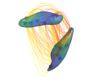
A procedure for extracting the community-based structure for turbulent flows is illustrated in figure 1. In what follows, we first introduce the network representation of vortical interactions in § 2. We introduce the network-based measure of node strength and community detection to identify influential nodes in §§ 2.1 and 2.2, respectively. The importance of the network-based measures is discussed within the context of a model problem of ideal point-vortex dynamics. We assess the influence of the identified nodes to modify the dynamics of a collection of discrete point vortices in § 3. We then employ the network community-based formulation to extract influential structures in two- and three-dimensional isotropic turbulence, described in § 4. The numerical set-ups are discussed in § 4.1. We characterize the vortical network of two- and three-dimensional isotropic turbulence in § 4.2. We then demonstrate the use of community-based structures to modify the turbulent flows in § 4.3. Finally, concluding remarks are provided in § 5.

Figure 1. An overview of the community-based procedure for extracting turbulent-flow-modifying structures.
2. Network-theoretic description of vortical interactions
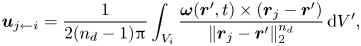
To identify the influential regions to perturb for flow modification, we examine the interactions amongst the vortical elements. We discretize the vorticity field in a Lagrangian and Eulerian perspective. The discrete vortical elements are referred to as nodes in the present work. To quantify the interactions amongst the vortical nodes, we consider the induced velocity imposed upon each other. The Biot–Savart law provides the induced velocity from a vortical element as a function of circulation and relative position of the vortical elements, expressed as
 \begin{equation} \boldsymbol{u}(\boldsymbol{r},t) = \frac{1}{2(n_{d}-1){\rm \pi}} \int_{V} \frac{\boldsymbol{\omega}(\boldsymbol{r}',t) \times (\boldsymbol{r}-\boldsymbol{r}')} {\|\boldsymbol{r}-\boldsymbol{r}'\|_2^{n_{d}}} \,\text{d}V', \end{equation}
where  $\boldsymbol {u}(\boldsymbol {r},t)$ is the induced velocity at location
  $\boldsymbol {r}$ in the domain from a collection of vortical elements enclosed in volume
  $V$ with a vorticity distribution of
  $\boldsymbol {\omega }(\boldsymbol {r}',t)$ at positions
  $\boldsymbol {r}'$. Here,
  $n_{d}$ is the spatial dimension of the flow field and
  $\|\cdot \|_2$ denotes the Euclidean norm. Furthermore, the influence of a vortical node (element)
  $i$ on node
  $j$ is evaluated as
 \begin{equation} \boldsymbol{u}_{j\leftarrow i} = \frac{1}{2(n_{d}-1){\rm \pi}} \int_{V_i} \frac{\boldsymbol{\omega}(\boldsymbol{r}',t) \times (\boldsymbol{r}_j-\boldsymbol{r}')} {\|\boldsymbol{r}_j-\boldsymbol{r}'\|_2^{n_{d}}} \,\text{d}V', \end{equation}
where  $\boldsymbol {u}_{j\leftarrow i}$ denotes the velocity induced from vortical node
  $i$ to
  $j$ and
  $V_i$ represents the volume of vortical node
  $i$. As an example, we illustrate the interactions between two vortical nodes in figure 2. The vortical structures are visualized by the isosurface of
  $Q$-criterion,
  $Q = \frac {1}{2}[ \| (\boldsymbol {\nabla } \boldsymbol {u} - \boldsymbol {\nabla } \boldsymbol {u}^{T}) \|_2^{2} - \| (\boldsymbol {\nabla } \boldsymbol {u} + \boldsymbol {\nabla } \boldsymbol {u}^{T}) \|_2^{2} ]$ (Hunt et al. Reference Hunt, Wray and Moin1988), and coloured with the magnitude of vorticity
  $\|\boldsymbol {\omega }\|_2$. Here, element
  $i$ has higher vorticity magnitude compared with element
  $j$. Thus, the magnitude of velocity induced by
  $i$ onto
  $j$ is higher than that imposed by
  $j$ onto
  $i$, yielding an asymmetric interaction.
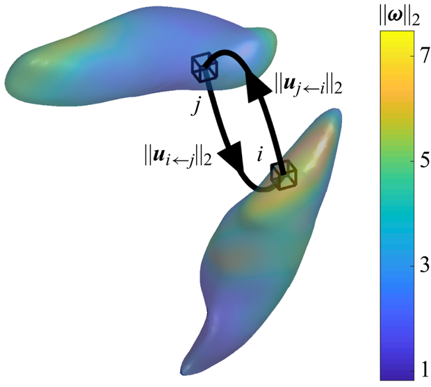
Figure 2. Interactions between two vortical elements in vortical structures extracted from three-dimensional isotropic turbulent flow. The vortical structures are visualized by isosurface of Q-criterion coloured with the magnitude of vorticity  $\|\boldsymbol {\omega }\|_2$. The vortical elements are shown for the spatial grid cells.
Characterizing the interaction-based behaviour of vortical elements can be a challenge in high-Reynolds-number turbulence, particularly with high degrees of freedom needed to discretize the flows. To facilitate the analysis of high-dimensional dynamics, we leverage the analytical approaches in graph theory (Bollobás Reference Bollobás1998) and network science (Newman Reference Newman2010). Here, we establish a network-theoretic representation of the vortical interactions in a flow field. We construct a network (graph)  $\mathscr {G}$ comprising vortical nodes
  $\mathscr {V}$ connected by edges
  $\mathscr {E}$ holding edge weights
  $\mathscr {W}$ based on induced velocity. Given this definition
  $\mathscr {G} = \mathscr {G}(\mathscr {V},\mathscr {E},\mathscr {W})$ for the network, we can quantify the important nodes in vortical flows.
The collection of connectivity amongst the nodes can be represented by the adjacency matrix  $\boldsymbol{\mathsf{A}}$, which holds the edge weights as its elements. For the vortical interaction network,
  $\boldsymbol{\mathsf{A}}$ is defined using the normalized magnitude of induced velocity (Nair & Taira Reference Nair and Taira2015; Taira et al. Reference Taira, Nair and Brunton2016) as
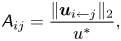 \begin{equation} {\mathsf{A}}_{ij} = \frac{\|\boldsymbol{u}_{i\leftarrow j}\|_2}{u^{*}}, \end{equation}
where  $u^{*}$ is a characteristic velocity of the flow. For a flow field with
  $n$ vortical nodes, the adjacency matrix
  $\boldsymbol{\mathsf{A}} \in \mathbb {R}^{n\times n}$. The above formulation gives an asymmetric adjacency matrix, representing a directed network. Adding directions to the links helps differentiate between the influential and influenced nodes. Non-dimensionalization is important for the analysis of turbulent flows over a range of Reynolds number. The details of the non-dimensionalization will be discussed in § 4.
Let us discuss the role of  $\boldsymbol{\mathsf{A}}$ on network dynamics and appropriate measures to identify influential nodes. Consider a general dynamical system for
  $n$ state vectors
  $\boldsymbol {x}_i \in \mathbb {R}^{p_{v}}$ holding
  $p_{v}$ variables over a network. The general interaction-based dynamics of the elements can be expressed as
 \begin{equation} \dot{\boldsymbol{x}}_i = \boldsymbol{f}(\boldsymbol{x}_i) + \sum_{j=1}^{n} {\mathsf{A}}_{ij} \boldsymbol{g}(\boldsymbol{x}_i, \boldsymbol{x}_j), \quad i = 1, 2, \ldots, n, \end{equation}
where function  $\boldsymbol {f}(\boldsymbol {x}_i)$ represents the intrinsic dynamics of node
  $i$ and function
  $\boldsymbol {g}(\boldsymbol {x}_i,\boldsymbol {x}_j)$ describes the interactive dynamics between nodes
  $i$ and
  $j$. We consider the model fluid-flow problem of ideal point-vortex dynamics (Aref Reference Aref2007; Newton Reference Newton2013) to demonstrate the interaction-based dynamics of vortical elements and identify important vortical nodes using the network-based approach.
Let us take a collection of  $n = 100$ discrete point vortices, initialized on an infinite two-dimensional domain as shown in figure 3(a). These vortices are initially arranged into five groups initial time instant. The vortices are coloured by their circulations
  $\varGamma _i=\omega _i \Delta S$, which is kept constant over time in the inviscid flow. Here, the vortical elements have the same area
  $\Delta S$. The circulations have a normal distribution about a mean of
  $\overline{\varGamma } = 0.1$ and a standard deviation of
  $\sigma _{\varGamma } = 0.008$. This canonical model problem portrays the nonlinear dynamics of vortical structures found in various flows (Nair & Taira Reference Nair and Taira2015). The transparent grey edges visualize all interactions amongst the nodes, based on (2.3). Here, we use
  $u^{*} = |\varGamma _{{tot}}|/(2{\rm \pi} R_0)$ where
  $\varGamma _{{tot}} = \sum _i^{n} \varGamma _i$ is the total circulation of the system and
  $R_0$ is the average radial distance of the centroid of the clusters from the geometric centre of the overall system at initial condition. The spatial variables are non-dimensionalized by
  $R_0$. The Biot–Savart law governs the dynamics of the point vortices, which can be expressed in terms of (2.4) for which
  $\boldsymbol {f}(\boldsymbol {r}_i) = 0$,
  ${\mathsf{A}}_{ij} = |\varGamma _j|/(2{\rm \pi} u^{*} \|\boldsymbol {r}_i - \boldsymbol {r}_j\|_2 )$ and
  $\boldsymbol {g}(\boldsymbol {r}_i, \boldsymbol {r}_j) = u^{*} \hat {\boldsymbol {k}}\times (\boldsymbol {r}_i - \boldsymbol {r}_j)/\|\boldsymbol {r}_i - \boldsymbol {r}_j\|_2$. Here,
  $\hat {\boldsymbol {k}}$ is the out-of-plane unit normal vector. We use this dynamical systems example to demonstrate the evaluation of important network measures pertinent to the interactive dynamics of the vortical elements.
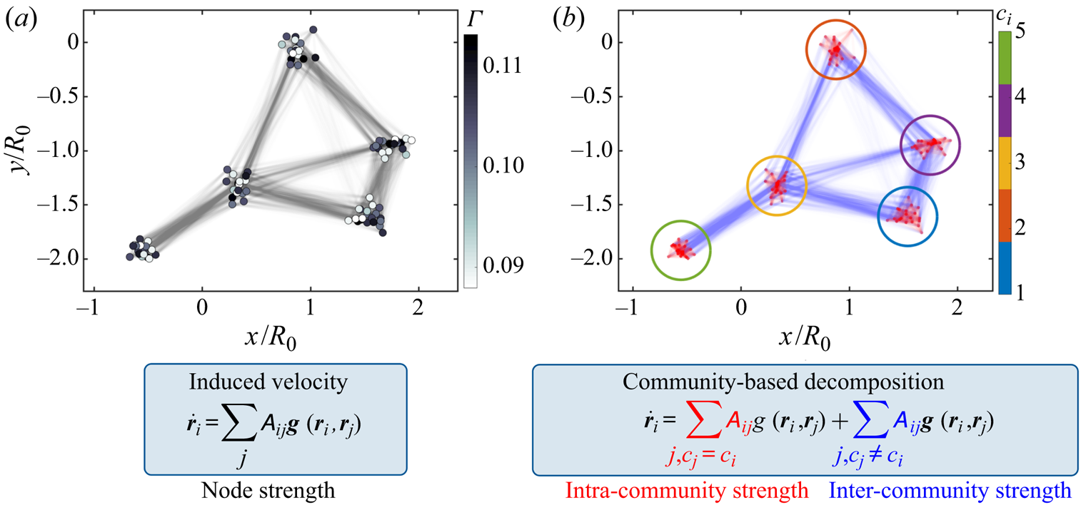
Figure 3. Interactions amongst a collection of discrete point vortices are used to illustrate the decomposition of networked dynamics through intra- and inter-community interactions.
2.1. Node strength
The node strength measures the ability of a node to be influential (out-strength) or be influenced (in-strength) in the network. The out- and in-strengths of a node are defined by
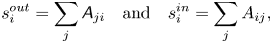 \begin{equation} s_i^{out} = \sum_{j}{\mathsf{A}}_{ji} \quad \text{and} \quad s_i^{in} = \sum_{j}A_{ij}, \end{equation}
respectively. These measures are useful to identify the node with a collection of significant connections in a network.
For the vortical networks, the present definition of edge weight from (2.3) is based on the out-weight, which is used to evaluate the out-strength. Herein, the node strength,  $s_i$, is taken to be the out-strength, unless specified otherwise. A relation between the node strength and enstrophy,
  $\varOmega (\boldsymbol {r},t) = \|\boldsymbol {\omega }(\boldsymbol {r},t)\|_2^{2}$, of a vortical element can be obtained using (2.2) as
 \begin{align} s_i &= \frac{1}{2(n_{d}-1){\rm \pi} u^{*}} \sum_j \left\|\int_{V_i} \frac{\boldsymbol{\omega}(\boldsymbol{r}',t) \times (\boldsymbol{r}_j-\boldsymbol{r}')} {\|\boldsymbol{r}_j-\boldsymbol{r}'\|_2^{n_{d}}} \,\text{d}V'\right\|_2 , \end{align}
 \begin{align} &\cong \frac{1}{2(n_{d}-1){\rm \pi} u^{*}} \sum_j \left\| \int_{S_i}{\|\boldsymbol{\omega}(\boldsymbol{r}',t)\|_2 \hat{\boldsymbol{e}}_{\boldsymbol{\omega}( \boldsymbol{r}',t)} \,\text{d}S'} \times \frac{(\boldsymbol{r}_j-\boldsymbol{r}_i)} {\|\boldsymbol{r}_j-\boldsymbol{r}_i\|_2^{n_{d}}}\Delta l_i\right\|_2 , \end{align}
 \begin{align} &=\frac{|\varGamma_i| \Delta l_i}{2(n_{d}-1){\rm \pi} u^{*}} \sum_j \frac{\| \hat{\boldsymbol{e}}_{\boldsymbol{\omega}_i} \times \hat{\boldsymbol{e}}_{\boldsymbol{r}_j-\boldsymbol{r}_i}\|_2} {\|\boldsymbol{r}_j-\boldsymbol{r}_i\|_2^{(n_{d}-1)}}, \end{align}
 \begin{align} &=\frac{\sqrt{\varOmega_i} \Delta V_i}{2(n_{d}-1){\rm \pi} u^{*}} C, \end{align}
where  $\hat {\boldsymbol {e}}_{(\cdot )}$ denotes the unit vector in the direction of
  $(\cdot )$,
  $\Delta l_i$ is the length of vortical element
  $i$, and the sum of distance components is denoted by
  $C=\sum _j\| \hat {\boldsymbol {e}}_{\boldsymbol {\omega }_i} \times \hat {\boldsymbol {e}}_{\boldsymbol {r}_j-\boldsymbol {r}_i}\|_2/ \|\boldsymbol {r}_{j}-\boldsymbol {r}_{i}\|_2^{(n_{d} - 1)}$, which is constant for a fully periodic domain. Here, we assume that the vortical element
  $j$ is sufficiently distant from the vortical element
  $i$ such that
  $(\boldsymbol {r}_j-\boldsymbol {r}')/\|\boldsymbol {r}_j-\boldsymbol {r}'\|_2^{n_{d}}$ is constant over the vorticity concentration of
  $i$, giving rise to (2.6b) (Kundu, Cohen & Dowling Reference Kundu, Cohen and Dowling2011). This relationship reveals that
  $s_i \propto \sqrt {\varOmega _i}$. This is particularly useful to determine the node strength distribution
  $p(s)$ of a vortical network, computation of which becomes prohibitively expensive for networks comprising large number of edges, such as turbulent flows of high Reynolds number. The distribution is dependent on the enstrophy distribution
  $p(\varOmega )$. The latter is usually a known or measurable flow statistics. Distribution
  $p(s)$ gives a global picture of the nature of connectivity in the network and is used to identify the type of the network (Barabási Reference Barabási2016). The distribution is also useful to identify the node with the highest interaction strength,
  $\max _i s_i$, which is referred to as the hub node of a network. These nodes have been found to be important in assessing the robustness of the network dynamics against random and targeted perturbations (Albert, Jeong & Barabási Reference Albert, Jeong and Barabási2000; Taira et al. Reference Taira, Nair and Brunton2016).
2.2. Community detection
Identifying closely connected vortical nodes is important towards revealing key local groups on the network. Such modular groups of nodes with high connectivity amongst each other are referred to as communities (Newman & Girvan Reference Newman and Girvan2004). One approach to find the communities is to measure the overall modular nature of a network using modularity  $M$ (Leicht & Newman Reference Leicht and Newman2008) given by
 \begin{equation} M = \frac{1}{2n_{e}}\sum_{ij}\left[ {\mathsf{A}}_{ij} - \gamma_{M}\frac{s_i^{in}s_j^{out}}{2 n_{e}} \right] \delta(c_i,c_j), \end{equation}
where  $n_{e}$ is the total number of edges in the network,
  $\gamma _{M}$ is the modularity resolution parameter to weigh the presence of small or large communities in the network (Reichardt & Bornholdt Reference Reichardt and Bornholdt2006; Fortunato & Barthélemy Reference Fortunato and Barthélemy2007),
  $\delta (c_i,c_j)$ is the Kronecker delta,
  $c_i \in \hat {C}_k$ is the label of the community to which element
  $i$ is assigned and
  $\hat {C}_k$ is the set of
  $k$-th network community. Here,
  $k = 1,2, \ldots , m$, with
  $m$ being the total number of communities. The communities can be identified by maximizing
  $M$ by regrouping the nodes. Here, the number of communities
  $m$ is unspecified and determined by the algorithm. Various algorithms are available to identify the communities in a network (Fortunato Reference Fortunato2010). In the present study, we adopt the method by Blondel et al. (Reference Blondel, Guillaume, Lambiotte and Lefebvre2008) to identify the communities in large vortical networks with accuracy and low computational cost (Fortunato Reference Fortunato2010). We herein refer to these network communities on vortical networks as the vortical communities (Gopalakrishnan Meena et al. Reference Gopalakrishnan Meena, Nair and Taira2018). Also, for vortical flows,
  $\gamma _{M}$ can be set based on the plateau effect on the number of vortical communities identified with change in
  $\gamma _{M}$ for a given Reynolds number.
The community information can then be used to decompose the term with the adjacency matrix in (2.4) as
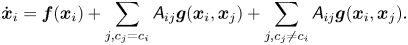 \begin{equation} \dot{\boldsymbol{x}}_i = \boldsymbol{f}(\boldsymbol{x}_i) + \sum_{j, c_j = c_i} {\mathsf{A}}_{ij} \boldsymbol{g}(\boldsymbol{x}_i,\boldsymbol{x}_j) + \sum_{j, c_j {\ne} c_i} {\mathsf{A}}_{ij} \boldsymbol{g}(\boldsymbol{x}_i,\boldsymbol{x}_j). \end{equation}
The second term on the right-hand side represents the interaction of node  $i$ with the nodes in its own community, and the third term denotes the interaction of node
  $i$ with the nodes in the other communities. The former represents the intra-community interactions and the latter term captures the inter-community interactions of node
  $i$. This gives a community-based dynamical systems equation for the elements of a network, emphasizing local influences of the communities. An illustration of the above procedure applied to the system of point vortices is shown in figure 3. The network with no distinction of the weighted edges is shown in figure 3(a). The community detection algorithm classifies the nodes into several communities, highlighted by the coloured circles in figure 3(b). The intra- and inter-community edges are shown in red and blue, respectively.
Let us quantify the local influence of a node using the above formulation. Similar to how the node strength is defined in (2.5a,b), the strength of node  $i$ to influence all nodes in community
  $k$ can be defined as
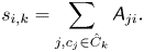 \begin{equation} s_{i,k} = \sum_{j,c_j \in \hat{C}_k} {\mathsf{A}}_{ji}. \end{equation}
Moreover, the strength of a node on the network can be separated into intra- and inter-community strengths as
 \begin{equation} s_{i}^{{intra}} = \sum_{j, c_j=c_i} {\mathsf{A}}_{ji} = s_{i,c_i} \quad \text{and} \quad s_{i}^{{inter}} = \sum_{j,c_j\!{\ne}\, c_i} {\mathsf{A}}_{ji} = \sum_{k,k \!{\ne}\, c_i}s_{i,k}, \end{equation}
respectively. These community-based strengths can be used to quantify the interactions with respect to communities.
The intra-community strength can be normalized as the within-module z-score (Guimera & Amaral Reference Guimera and Amaral2005) given by
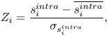 \begin{equation} Z_i = \frac{s_{i}^{{intra}} - \overline{s_{i}^{{intra}}}}{\sigma_{s_{i}^{{intra}}}}, \end{equation}
where  $\overline {s_{i}^{{intra}}}$ and
  $\sigma _{s_{i}^{{intra}}}$ are the mean and standard deviation of
  $s_{i}^{{intra}}$ over all nodes in the community of
  $i$. The within-module z-score identifies the most well-connected node inside a community or the hub node of a community. Note that the hub node of a community need not be well-connected with the other communities in the network.
A relative measure of inter-community strength of a node, quantified by how well-distributed its edges are amongst communities, can be given by the participation coefficient (Guimera & Amaral Reference Guimera and Amaral2005)
 \begin{equation} P_i = 1 - \left[ \left( \frac{s_{i}^{{intra}}}{s_i} \right) ^{2} + \sum_{k,k \!{\ne}\, c_i}\left( \frac{s_{i,k}}{s_i} \right) ^{2} \right]. \end{equation}
When  $P_i\approx 1$, edge weights of node
  $i$ are equally connected among all communities, and
  $P_i=0$ when the node is only connected to its own community. Note that
  $s_{i,k}$,
  $Z_i$ and
  $P_i$ can be evaluated for both in- and out-edges. In the present study, we evaluate the out-edge based measures following the definition of edge weight from (2.3).
The  $P$–
$P$– $Z$ map of a network, comprising
  $P_i$ and
  $Z_i$ values of all the nodes on the network, is an important feature space for revealing key elements within and amongst the communities (Guimera et al. Reference Guimera, Mossa, Turtschi and Amaral2005; Fortunato Reference Fortunato2010; Rubinov & Sporns Reference Rubinov and Sporns2010). The plot shows the
  $P_i$ and
  $Z_i$ values on the horizontal and vertical axes, respectively. This map identifies influential nodes based on their relative importance in influencing their own community and other communities in the network through intra- and inter-community interactions, respectively. For vortical networks, high intra-community influence of vortical elements can be understood as the ability to significantly affect the behaviour of their own vortical structure by imparting self-induced velocity on the other elements with the same structure. Whereas, high inter-community interaction of vortical elements can be interpreted as the ability to impart high induced velocity on other vortical structures.
The  $P$–
$P$– $Z$ map for the system of point vortices is shown in figure 4(a). The nodes on the left side of the
  $P$–
$P$– $Z$ map have very low inter-community interactions and are isolated groups, called peripherals. On the other hand, the nodes on the right side have high inter-community interactions, making them well-connected to most communities and are called connectors. The nodes on the top region with high
  $Z$ value have the strongest interactions within the respective communities. Note that the name peripheral need not refer to nodes at the physical perimeter of the domain. The strongest peripheral nodes will have high influence within their communities but the least influence on other communities. In contrast, the strongest connector nodes will have the highest influence amongst communities, particularly on the neighbouring communities (in spatial proximity), and high influence within their own community.
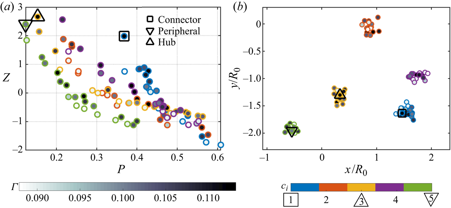
Figure 4. (a)  $P$–
$P$– $Z$ map for the discrete point vortices. The influential connector (
 $\square$), peripheral (
 ${\bigtriangledown}$) and hub (
 ${\bigtriangleup}$) nodes are also identified. (b) Position of the important nodes in physical space.
We use the  $P$–
$P$– $Z$ feature space to search for the strongest peripheral and connector nodes in a network, herein referred to as simply peripheral and connector nodes. We find the average
  $P_i$ of each community
  $k$, denoted as
  $\overline {P_k}$. The peripheral node of a network is the node
  $i$ given by
  $\max _{i,c_i=k}Z_i$, belonging to the community
  $k$ with
  $\min _{k}\overline {P_k}$. The connector node
  $i$ is given by
  $\max _{i,c_i=k}Z_i$, belonging to community
  $k$ with
  $\max _{k}\overline {P_k}$. The connector, peripheral, and hub nodes of the discrete point-vortex system are indicated in figure 4(a). The
  $P$–
$P$– $Z$ values for the nodes suggest that the hub node would have similar characteristics as the peripheral node. The three important nodes are also highlighted in the physical space as shown in figure 4(b). The positions of the peripheral and connector nodes suggest that an influential node need not be located at the geometric centre of the community. The observations signify the need to consider inter- and intra-community interactions for identifying important nodes. Let us now demonstrate how the behaviour of the networked system can be modified using these measures.
3. Community-based modification of discrete point-vortex dynamics
We analyse the influence of the connector, peripheral and hub nodes identified using the network-based measures on the dynamics of a collection of discrete point vortices. We consider the same model problem set-up with  $n=100$ discrete point vortices used in § 2. Velocity-based impulse perturbations are added to all nodes of the identified influential community. Based on the community being perturbed, we refer to the forcing input as connector, peripheral or hub-based perturbation. Positions of the perturbed communities at the initial time instant are shown in figure 4(b). We identify the influential nodes only at the initial time instant as we are interested in exploring the influence of the nodes on the system dynamics.
Impulse perturbations at discrete time  $n_{t}\Delta t$ are added to the velocity field with time step
  $\Delta t$ and
  $n_{t} = 0,1,2,\ldots$ . The velocity of a perturbed node
  $i$ at time
  $t$ is given by
  $\boldsymbol {u}(\boldsymbol {r}_i,t) + \tilde {\boldsymbol {u}}(\boldsymbol {r}_i,t)$, where
  $\tilde {\boldsymbol {u}}(\boldsymbol {r}_i,t) = \alpha \hat {e}_{\boldsymbol {u}(\boldsymbol {r}_i,t)} \delta (t-n_{t}\Delta t)$,
  $\alpha$ is the amplitude of perturbation, and
  $\hat {e}_{\boldsymbol {u}(\boldsymbol {r}_i,t)}$ is the unit vector in the direction of
  $\boldsymbol {u}(\boldsymbol {r}_i,t)$. Time is non-dimensionalized as
  $t\varGamma _{{tot}}/(2{\rm \pi} R_0^{2})$. Amplitude of perturbation
  $\alpha$ is computed for a given energy ratio
  $E$ of
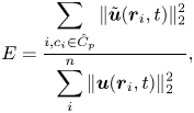 \begin{equation} E=\frac{\displaystyle\sum_{i,c_i\in \hat{C}_p} \| \tilde{\boldsymbol{u}}(\boldsymbol{r}_i,t) \|_2^{2}}{\displaystyle\sum_i^{n}\| \boldsymbol{u}(\boldsymbol{r}_i,t)\|_2^{2}}, \end{equation}
where  $\hat {C}_p$ is the set of the perturbed community. We have analysed the system dynamics with
  $E$ varied between 0.01–0.1 and have found qualitative similarity in the results. Here, we show the results of perturbations with
  $E=0.1$ to portray significant changes in the vortex trajectories. The time step between each perturbation is
  $\Delta t\varGamma _{{tot}}/(2{\rm \pi} R_0^{2}) = 0.024$.
The effect of the perturbations on system dynamics is assessed by observing the change in trajectories of the community centroids, as shown in figure 5(a–c). The centroid location  $\boldsymbol {\xi }_k(t)$ of each community
  $k$ is computed as
 \begin{equation} \boldsymbol{\xi}_k(t) = \frac{\displaystyle\sum_{i,c_i\in \hat{C}_k} \varGamma_i \boldsymbol{r}_i(t)}{\displaystyle\sum_{i,c_i\in \hat{C}_k}\varGamma_i}. \end{equation}
The connector-based perturbations achieve the largest deviations on the trajectories as shown in figure 5(a). The peripheral and hub-based perturbations have significant influence only on their neighbouring communities, communities  $3$ and
  $1$, respectively, as evident from figures 5(b) and 5(c). Regardless of the central location of the hub community at the initial time instant, the system dynamics is not changed compared with the extent achieved by connector-based perturbations. This demonstration highlights the need to consider the strengths and relative positions in a systematic manner to identify the influential nodes.
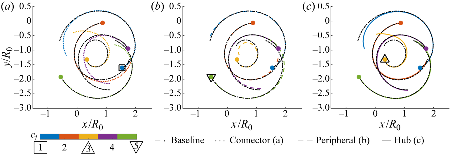
Figure 5. Trajectories of community centroids with perturbations added to (a) connector ( $\square$), (b) peripheral (
 ${\bigtriangledown}$) and (c) hub (
 ${\bigtriangleup}$) communities. Filled circles show initial position of the community centroids.
Let us compare the community centroid trajectories in time, as shown in figure 6(a). The trajectories of all other communities show the most deviation from baseline with connector-based perturbation, except for community 5. The trajectory of community 5, the peripheral community, is modified significantly when it is perturbed. We have evaluated the  $P$–
$P$– $Z$ map using the in-edges (not shown), which also gives community 5 to be the peripheral community. Thus, other communities have less influence on community 5. We concentrate on the results during early time instants to assess the characteristics of the connector to influence its neighbour and connect with other communities. The trajectory of community
  $4$ is changed significantly at early time instants with connector-based perturbations. This change in trajectory of community 4, the spatially closest community to the connector, at early time instants demonstrates the ability of a connector community to significantly influence its neighbour. Neither of the peripheral and hub-based perturbations influence other communities, particularly their respective neighbours, at early times. Later, the connector-based perturbations also significantly change the dynamics of community
  $3$ by connecting through community
  $4$, even though communities
  $1$ and
  $3$ are spatially far apart. The inter-community influence demonstrates the connecting characteristics of a connector community.
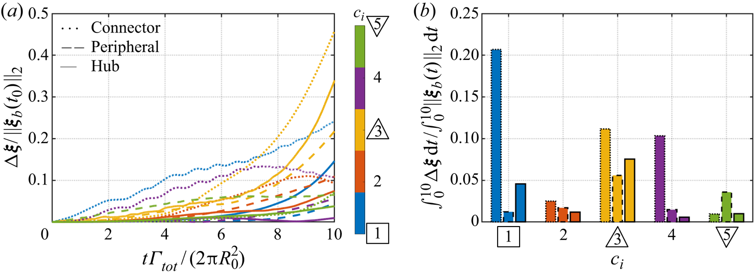
Figure 6. (a) Trajectories of community centroids subjected to connector ( $\square$), peripheral (
 ${\bigtriangledown}$) and hub-based (
 ${\bigtriangleup}$) perturbations compared with baseline,
  $\boldsymbol {\xi }_b$. Here,
  $\Delta \boldsymbol {\xi } = \| \boldsymbol {\xi }(t) - \boldsymbol {\xi }_b(t) \|_2$. (b) Total change in trajectory of community centroids with respect to the baseline.
Deviation of the trajectories from baseline is quantified in figure 6(b). The observations quantitatively show the larger deviations in trajectories resulting from connector-based perturbations. Considering the neighbours of the perturbed communities, a total change between 10–12 % of the baseline is achieved for communities  $3$ and
  $4$ using connector-based perturbations. The corresponding changes using peripheral and hub-based perturbations are around
  $5\,\%$ for communities
  $3$ and
  $1$, respectively. The largest effect of the hub community is on its own trajectory. These observations demonstrate the inference from the
  $P$–
$P$– $Z$ map that the hub community can portray characteristics of a peripheral. The magnitude of change achieved by the connector-based perturbation on its own trajectory is more than three times that produced by peripheral and hub communities. Furthermore, the total change in trajectory of community
  $3$ is the highest using connector-based perturbation. For this model problem, we have demonstrated that the connector node effectively modifies the global vortex dynamics. The present finding motivates the use of inter-community interactions to instigate changes in the global system dynamics, based on the community-based decomposition of system dynamics to identify key structures.
4. Community-based flow modification of isotropic turbulence
Let us now consider the application of community-based flow modification to two- and three-dimensional decaying homogeneous isotropic turbulence. The highly complex and multiscale properties of isotropic turbulence make it an apt choice to demonstrate the capability of the present community-based framework. Isotropic turbulence is a canonical model problem for a range of turbulent flows encountered in nature and engineering applications.
4.1. Numerical set-up
For the two- and three-dimensional decaying isotropic turbulent flows, we use the Fourier spectral and pseudo-spectral algorithms, respectively, to numerically solve the Navier–Stokes equations (Chumakov Reference Chumakov2008; Taira et al. Reference Taira, Nair and Brunton2016). Direct numerical simulations (DNS) of the unforced flows are performed in bi-periodic and tri-periodic square and cubic domains of length  $L$. For the simulations, the flow fields are resolved such that
  $k_{{max}}\eta \geqslant 1$, where
  $k_{{max}}$ is the maximum resolvable wavenumber of the grid and
  $\eta$ is the Kolmogorov length scale. We non-dimensionalize the spatial variables by
  $L$ and time by the large-eddy turn-over time at the initial time instant
  $\tau _e(t_0)$.
The two-dimensional DNS are initialized with a smooth distribution comprising approximately  $100$ superimposed Taylor vortices with random strengths, core sizes and locations. The flow field satisfies the kinetic energy spectra
  $E(k) \propto k \exp (-k^{2}/k_0^{2})$, where
  $k_0=26.5$ (Kida Reference Kida1985; Brachet, Meneguzzi & Sulem Reference Brachet, Meneguzzi and Sulem1986). The three-dimensional DNS are initialized with random velocity fields of Gaussian p.d.f. profiles satisfying incompressibility and the Kolmogorov spectra for kinetic energy,
 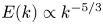 $E(k) \propto k^{-5/3}$. The two- and three-dimensional simulations are run from these initial conditions until the flows are in the decaying regime, after which data are collected to perform the network analysis.
The two-dimensional turbulent flows with an initial Taylor microscale-based Reynolds number of 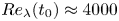 $Re_\lambda (t_0) \approx 4000$ are obtained from DNS performed at a grid resolution of
  $1024\times 1024$. We use snapshots of the vorticity field, uniformly subsampled to a resolution of
  $128\times 128$, to construct the vortical network. For three-dimensional isotropic turbulence, flow fields with
  $Re_\lambda (t_0) \approx 40$ are obtained from DNS performed with a grid resolution of
  $64 \times 64 \times 64$. The three-dimensional flow fields are uniformly subsampled to a resolution of
  $32\times 32\times 32$ for constructing the vortical network. Subsampling is performed in a manner such that the network representation is not influenced.
The network representation can be made independent of the Reynolds number following the non-dimensionalization of the edge weights using (2.3). We choose the characteristic velocity
 \begin{equation} u^{*} = V^{1/n_{d}}\varOmega_{{tot}}^{1/2} = V^{1/n_{d}} \left(\frac{\displaystyle\int_{\|\boldsymbol{\omega}\|_2\geqslant\omega_{{th}}} \|\boldsymbol{\omega}(\boldsymbol{r},t)\|_2^{2} \,\text{d}V}{V}\right)^{1/2}, \end{equation}
where  $\varOmega _{{tot}}$ is the total enstrophy per unit area or volume of all the vortical elements enclosed in a region of vorticity threshold
  $\omega _{th}$. We concentrate on vortical elements with high vorticity (McWilliams Reference McWilliams1984), extracted through vorticity thresholding (Jiménez et al. Reference Jiménez, Wray, Saffman and Rogallo1993). We can capture the overall interaction behaviour of the flow field even with the threshold. For both two- and three-dimensional flow fields, we use a threshold of
  $\omega _{th}=0.05||\boldsymbol {\omega }(\boldsymbol {r})||_\infty$. Detailed assessment on the influence of the Reynolds number, grid and
  $\omega _{th}$ is provided in the Appendix.
4.2. Network characterization of isotropic turbulence
Let us first characterize the interactions amongst the vortical elements in two- and three-dimensional isotropic turbulence. Following (2.6), we evaluate the node strength and enstrophy distributions of the flow fields at an instant in time, presented in figure 7. The enstrophy and square of node strength are normalized by their respective mean values. The node strength-enstrophy relations from (2.6) are shown here for isotropic turbulence. Benzi, Patarnello & Santangelo (Reference Benzi, Patarnello and Santangelo1987) found a power-law profile for the enstrophy distribution of two-dimensional decaying isotropic turbulence. The distribution  $p(s^{2})$ also follows a power-law behaviour as observed in figure 7(a). Taira et al. (Reference Taira, Nair and Brunton2016) analysed the network structure of two-dimensional decaying isotropic turbulence and found the undirected node strength (average of in- and out-strength) distribution
  $p(s)$ to follow a scale-free behaviour if the energy spectrum follows the
  $k^{-3}$ profile.
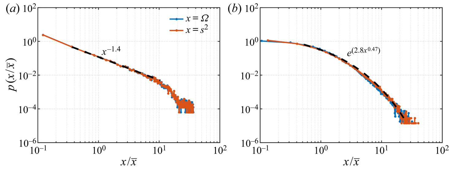
Figure 7. Probability distributions of enstrophy and node strength (squared), normalized by their mean values, of (a) two- and (b) three-dimensional isotropic turbulence.
For three-dimensional isotropic turbulence, the enstrophy distribution follows a stretched-exponential profile of the form  $p(\varOmega) \propto \exp(-a_\varOmega \varOmega^b)$, with
  $a_\varOmega$ and
  $b$ denoting the prefactor and exponent, respectively (Zeff et al. Reference Zeff, Lanterman, McAllister, Roy, Kostelich and Lathrop2003; Donzis, Yeung & Sreenivasan Reference Donzis, Yeung and Sreenivasan2008). We observe a stretched-exponential profile for
  $p(s^{2})$ with the same exponent
  $b$ as that of the enstrophy distribution, as shown in figure 7(b). The difference of
  $p(s^{2})$ for two- and three-dimensional flows can be attributed to the components of vorticity. For three-dimensional turbulence, vorticity is spread over wide scales of structures due to vortex stretching and tilting, which are absent in two-dimensional flows.
The node strength distributions can be used to highlight vortical elements with high node strength, as shown in figure 8. Isocontours of node strength, positive  $Q$-criterion and magnitude of strain rate tensor
  $\|\boldsymbol{\mathsf{S}}\|_2$, for the two- and three-dimensional flow fields are shown. For both flows, the high node strength regions align with those of high positive
  $Q$-criterion (vortex core) and
  $\|\boldsymbol{\mathsf{S}}\|_2$ (high shear regions). The node strength-enstrophy relation attributes to the alignment of the node strength with the
  $Q$ and
  $\|\boldsymbol{\mathsf{S}}\|_2$ measures in physical space. The observations show that the network-based node strength can indeed identify strong vortex cores and shear layers in turbulent flows.
Figure 8. Comparing vortical structures with high node strength (grey contours),  $Q$-criterion (red-yellow contours) and strain (blue-green contours) for (a) two- and (b) three-dimensional isotropic turbulence. Only a slice is shown for (b).
Let us now use the community-based framework to extract vortical communities in isotropic turbulence and identify influential regions to modify the flow using inter- and intra-community strength measures. A demonstration of the community detection algorithm and the corresponding  $P$–
$P$– $Z$ map applied to a three-dimensional flow field are shown in figure 9(a,b). Here, the initial community detection procedure coarsely identifies regions in the flow field. The flow field portrayed in figure 9(a) only shows regions of high vorticity above a vorticity threshold,
  $\omega _{{th}}$. A clear distinction between connectors and peripherals is not observed using the
  $P$–
$P$– $Z$ map. The continuous nature of the flow field and vortical structures being spatially close to each other can make it challenging for the community detection algorithm to extract distinct vortical structures. Similar observations were made in a previous study for laminar wakes (Gopalakrishnan Meena et al. Reference Gopalakrishnan Meena, Nair and Taira2018). The analysis of complex problems, such as turbulence through network science tools, requires providing physical intuitions to the network-based tools. A naive use of network-theoretic techniques may not necessarily reveal interaction-based characteristics of such complex systems since turbulent flows possess dense networks which are significantly different from most networks studied in network science.
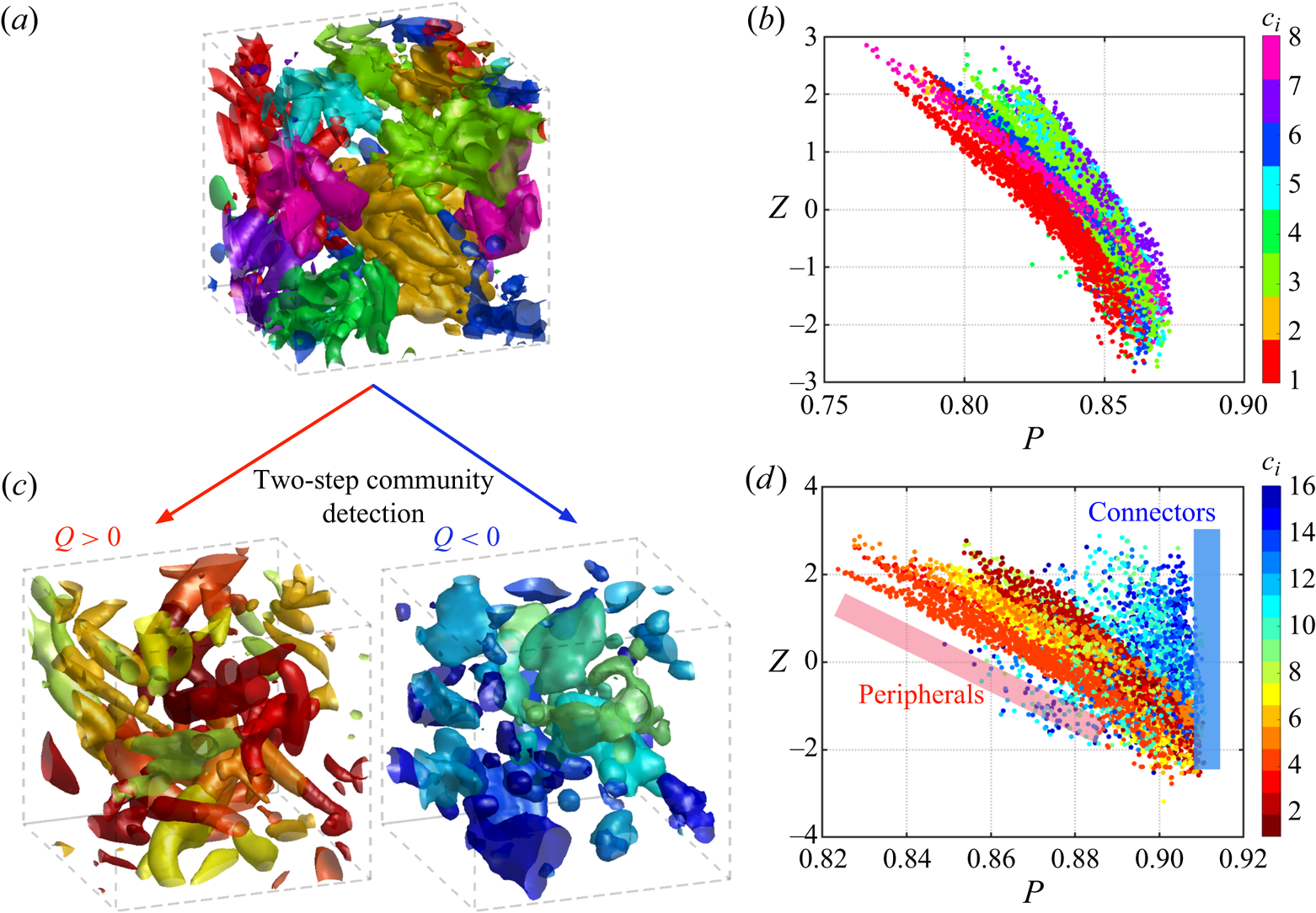
Figure 9. (a) Community detection in a three-dimensional isotropic turbulence and (b) the corresponding  $P$–
$P$– $Z$ map. (c) Two-step community detection and (d) the corresponding
  $P$–
$P$– $Z$ map. Connector and peripheral communities have distinct distributions in the
  $P$–
$P$– $Z$ map.
We aid the community detection algorithm by decomposing the flow field into nodes with  $Q>0$ and
  $Q<0$. This is portrayed in figure 9(c). The communities are identified independently for the two networks. The difference in the number of communities compared with the first step is due to the value of
  $\gamma _{M}$ used, which was found to be similar for both the steps for the given
  $Re_\lambda$. The new community labels are used to evaluate the
  $P$–
$P$– $Z$ map for the full adjacency matrix, as shown in figure 9(d). The two-step community detection procedure reveals the communities to broadly follow two correlations in the
  $P$–
$P$– $Z$ map. The communities on the left side of the map possess a negative correlation in the
  $P$–
$P$– $Z$ feature space and the nodes on the left side exhibit no significant correlation. We classify the former as peripheral and later as connector communities. The first group predominantly contains nodes with
  $Q>0$, the second group with
  $Q<0$. Thus, most peripheral and connector communities resemble vortex-core and shear-layer-type structures, respectively. Vortex cores that are spatially isolated in the flow can attribute to their classification as peripherals. Whereas, most shear-layer-type structures being located amongst vortical structures make them connectors. We observe similar results for two-dimensional isotropic turbulence and for other cases at various
  $Re_\lambda$. Given the classification of vortical structures into connector and peripheral communities, we can now identify the important communities and analyse their influence on the flow field.
4.3. Community-based flow modification
We compute the  $\overline {P_k}$ of each community
  $k$ to quantify the strength of influence. The connector and peripheral communities are the ones with
  $\max _k \overline {P_k}$ and
  $\min _k \overline {P_k}$, respectively, as highlighted in figure 10(a). The dominant nodes of the communities are determined based on
  $Z$. The peripheral community corresponds to the vortical structure visualized in red and the connector community comprising low circulation multivortical structures with both strain and rotational regions visualized in blue in figure 10(b).
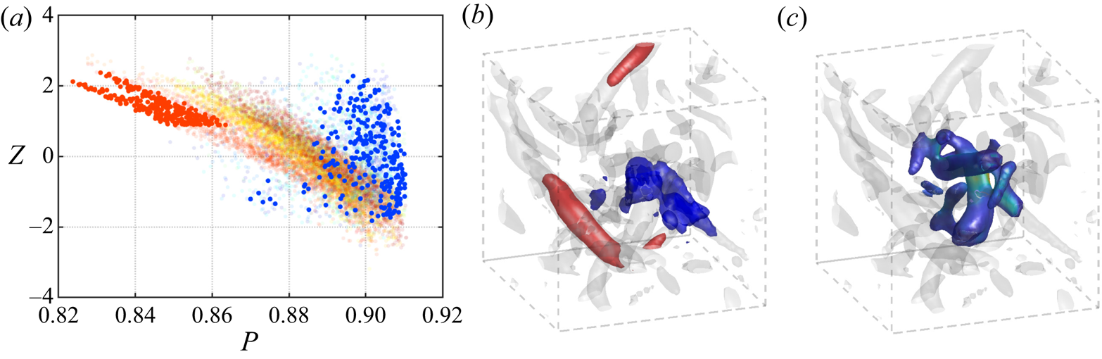
Figure 10. (a) Identification of the connectors and peripherals in the  $P$–
$P$– $Z$ map and (b) their structures in physical space. The red and blue colours denote the vortical structures corresponding to the strongest peripheral and connector communities, respectively. The transparent grey isosurfaces of
  $Q$-criterion represent the background flow field (vortical cores) for reference. (c) Local region around the connector structure, which is one integral length scale around the centroid of the structure.
We compare the influence of the connector structure to modify the flow with the strongest vortex tube and shear-layer-based regions, which are known to cause many flow modifications. The vortex tube and shear-layer structures are identified by large amplitudes of  $Q>0$ and
  $Q<0$, respectively. Herein, notations
  $Q^{+}$ and
  $Q^{-}$ are correspondingly used to denote the strongest vortex tube and shear-layer structures in the flow field. We do not present cases for the peripheral structures as they usually align with
  $Q^{+}$.
We add perturbations to the nodes identified as influential structures and track the changes to the flow. Impulse perturbations at discrete time  $n_{t}\Delta t$ are added to the velocity field with time step
  $\Delta t$ and
  $n_{t} = 0,1,2,\ldots$ . The perturbed velocity field at time
  $t$ is given by
  $\boldsymbol {u}(\boldsymbol {r},t) + \tilde {\boldsymbol {u}}(\boldsymbol {r},\boldsymbol {r}^{*},t)$, where
  $\tilde {\boldsymbol {u}}(\boldsymbol {r},\boldsymbol {r}^{*},t) = \alpha \tilde {\boldsymbol {f}}(\boldsymbol {r},\boldsymbol {r}^{*},t)$,
  $\alpha$ is the amplitude of the perturbation added to the perturbation
  $\tilde {\boldsymbol {f}}(\boldsymbol {r},\boldsymbol {r}^{*},t)$ and
  $\boldsymbol {r}^{*}$ is the location of the influential structure. The perturbation is given by
 \begin{equation} \boldsymbol{f}(\boldsymbol{r},\boldsymbol{r}^{*},t) = \frac{\hat{\boldsymbol{e}}_{\boldsymbol{u}(\boldsymbol{r},t)}}{\sqrt{2{\rm \pi}\Delta V^{2}}} \sum_{i=1}^{n_{p}} \exp\left( \frac{-\| \boldsymbol{r} - \boldsymbol{r}^{*}_i \|_2^{2}}{2\Delta V^{2}} \right) \delta(t - n_{t}\Delta t), \end{equation}
where  $\hat {\boldsymbol {e}}_{\boldsymbol {u}(\boldsymbol {r},t)}$ is the unit vector in the direction of
  $\boldsymbol {u}(\boldsymbol {r},t)$,
  $\Delta V$ is the volume of the vortical node (grid size) and
  $\boldsymbol {r}^{*}_i$ are the locations of all the
  $n_{p}$ perturbed nodes of the influential structure. We normalize
  $\boldsymbol {f}(\boldsymbol {r},\boldsymbol {r}^{*},t)$ to give
  $\tilde {\boldsymbol {f}}(\boldsymbol {r},\boldsymbol {r}^{*},t)$ such that
  $\int _V\|\tilde {\boldsymbol {f}}(\boldsymbol {r},\boldsymbol {r}^{*},t)\|_2^{2}\,\text {d}V = 1$. A prescribed forcing energy
  $E$ of
 \begin{equation} E=\frac{\displaystyle\int_V \| \tilde{\boldsymbol{u}}(\boldsymbol{r},\boldsymbol{r}^{*},t) \|_2^{2} \, \text{d}V}{\displaystyle\int_V \|\boldsymbol{u}(\boldsymbol{r},t) \|_2^{2}\, \text{d}V} \end{equation}
is used to compute the amplitude of perturbation  $\alpha$.
We first analyse the influence of the structures with a single perturbation added to all the nodes of the influential structures at the initial time instant. The perturbation amplitude is chosen such that  $E=0.04$, which is a reasonable magnitude for control. Based on the observations, we then employ multiple pulses to the nodes of the influential structures at time periodic instances
  $n_{t}\Delta t$. These influential structures are tracked in time for given isocontours (or isosurfaces) of
  $Q$-criterion and are subjected to impulse perturbations with time step normalized by the large eddy turn-overtime at the initial time instant,
  $\Delta t/\tau _e(t_0) =1$ and
  $0.2$ for two- and three-dimensional flows, respectively. We have chosen the time step for these turbulent flows based on the single perturbation analysis to obtain significant flow modification. The difference in time step for two- and three-dimensional isotropic turbulence is to consider the distinct predictability horizon of small-scale motion in the flows (Métais & Lesieur Reference Métais and Lesieur1986; Lesieur & Métais Reference Lesieur and Metais1996; Machiels Reference Machiels1997). While the two-dimensional flow would have predictability horizons spanning over a few eddy turn-over times, the present three-dimensional flow has a shorter time horizon. Herein, we refer to the experiments with perturbations at the initial time instant and multiple pulses at time periodic instances as single and multiple perturbations, respectively.
We concentrate on the flow evolution cases in the vicinity of the perturbed structures, one integral length scale around the centroid of the perturbed structure, as shown in figure 10(c). The peripheral-based or  $Q^{+}$ perturbations increase the circulation of the vortex core. In contrast, modification of the behaviour of multiple vortical structures by the connector-based and
  $Q^{-}$ perturbations enhances local mixing in the flow, as we discuss below. Based on the observations from the present study (for which the influential structures are identified only at the initial time instant), we have also performed preliminary analyses with the structure identification procedure repeated as the flow evolves. We observe similar results showing perturbation of the connector structures significantly enhancing turbulent mixing compared with perturbing
  $Q^{+}$ and
  $Q^{-}$ structures. In the present study, we concentrate on the structures identified at the initial time instant to characterize the influence of the network-based structures on turbulence.
Mixing enhancement in turbulent flows plays a key role in various engineering applications. Mixing enhancement by stirring has been attributed to generation of shear dominated filaments in the flow field (Spencer & Wiley Reference Spencer and Wiley1951; Aref Reference Aref1984; Ottino Reference Ottino1990; Eggl & Schmid Reference Eggl and Schmid2018). Here, we analyse the effect of the perturbations to enhance local mixing in isotropic turbulence based on the present network-based framework. We use fluid-particle tracking to quantify local mixing in the flow field. To quantify mixing, we consider the use of two-species fluid tracking (Coppola, Sherwin & Peiró Reference Coppola, Sherwin and Peiró2001). The first species is initialized one integral length scale around the centroid of the perturbed structure, the region previously shown in figure 10(c), and the second over the rest of the flow field. Given the velocity field  $\boldsymbol {u}(\boldsymbol {r},t)$, the time evolution of the fluid particle at
  $\boldsymbol {r}_p$ is given by
 \begin{equation} \frac{\text{d}\boldsymbol{r}_p}{\text{d}t} = \boldsymbol{u}(\boldsymbol{r}_p,t). \end{equation}
A second-order accurate Runge–Kutta scheme is implemented for time integration (Yu et al. Reference Yu, Kanov, Perlman, Graham, Frederix, Burns, Szalay, Eyink and Meneveau2012).
Local mixing is quantified by measuring the information entropy using the two species of particles in the domain (Kang & Kwon Reference Kang and Kwon2004; Cookson, Doorly & Sherwin Reference Cookson, Doorly and Sherwin2019). The flow field is discretized into cells and the entropy of the two species of particles is evaluated for each cell. The total information entropy of the whole domain at an instant in time is given by
 \begin{equation} S ={-} \sum_{i=1}^{n_{c}}\left [ w_i \sum_{k=1}^{2} ( n_{i,k} \log{n_{i,k}} ) \right ], \end{equation}
where  $n_{c}$ is the number of cells with which the full domain is discretized,
  $n_{i,k}$ is the number of particles of
  $k$th species in
  $i$th cell and
  $w_i$ is the weight factor. If the
  $i$th cell contains no particles or only particles of a single species,
  $w_i=0$, else
  $w_i=1$. Moreover, the relative entropy measure
  $\kappa$ (Kang & Kwon Reference Kang and Kwon2004) is given by
 \begin{equation} \kappa(t) = \frac{S(t) - S(t_0)}{S_{{max}} - S(t_0)}, \end{equation}
where  $S(t_0)$ is the entropy for initial particle distribution and
  $S_{{max}}$ is the maximum possible entropy increase over the domain, which is achieved when each cell contains equal number of particles of each species. For each perturbation set-up, we normalize
  $\kappa$ by the baseline
  $\kappa _{{base}}$ as
  $\tilde {\kappa }(t) = [ \kappa (t) - \kappa _{{base}}(t) ] / \| \kappa _{{base}}(t) \|_{\infty }$, thus measuring the mixing enhancement compared with the baseline flow. The baseline flow field is initialized with particles in the same pattern as each perturbed simulation to evaluate the respective
  $\kappa _{{base}}$.
Ensemble averages of  $\tilde {\kappa }$ for connector,
  $Q^{+}$, and
  $Q^{-}$-based perturbations performed on a number of two- and three-dimensional isotropic turbulent flows are shown in figure 11. For the two-dimensional isotropic turbulence with a single perturbation at the initial time instant, the connector-based perturbation achieves mixing enhancement similar to that of
  $Q^{-}$. Both connector-based and
  $Q^{-}$ perturbations outperform
  $Q^{+}$ for local mixing enhancement. With multiple pulses, connector-based perturbation generates entropy two times compared with the baseline flow, which is
  $54\,\%$ more than the
  $Q^{-}$ perturbations. The perturbation using
  $Q^{+}$ just leads to strengthening of vortex cores without significant spreading of particles, which will be visualized shortly.
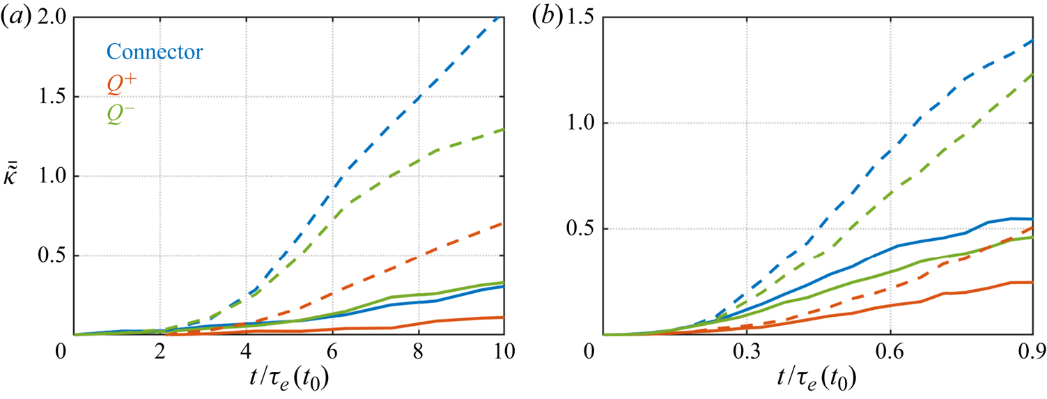
Figure 11. Ensemble average of normalized relative particle entropy in time for (a) two- and (b) three-dimensional isotropic turbulent flows subjected to connector-based,  $Q^{+}$, and
  $Q^{-}$ perturbations. Lines — denote results for single perturbation and
  $--$ for multiple perturbation cases. Ensemble is computed using 10 cases.
Using the results of two-dimensional flows as a guideline, we perform the analysis on three-dimensional flows, as shown in figure 11(b). A single pulse added to the connector at the initial time instant generates  $\tilde {\kappa }$ values
  $0.55$ times that of the baseline flow, which is
  $20\,\%$ more than the
  $Q^{-}$ perturbation. With multiple pulses, connector-based perturbations increase the entropy by
  $1.4$ times compared with the baseline flow, which is
  $17\,\%$ more than the
  $Q^{-}$ perturbations. Multiple pulses of
  $Q^{+}$ perturbation under-performs compared with even the single connector-based perturbation. According to the studies on mixing enhancement using stirrers (Aref Reference Aref1984; Eggl & Schmid Reference Eggl and Schmid2018), we expect the
  $Q^{-}$ perturbation to achieve better mixing. The present results are in agreement with these studies. Moreover, the connector-based perturbation outperforms the
  $Q^{-}$ perturbation, highlighting the capability of the network-theoretic framework to identify structures to effectively modify the flow.
With the above observations quantifying the effectiveness of connectors to modify turbulence and enhance local turbulence mixing, let us analyse the flow fields. We consider the time evolution of a two-dimensional isotropic decaying turbulent flow subject to multiple pulses of connector-based,  $Q^{+}$, and
  $Q^{-}$ perturbations, as shown in figure 12. The flow field is visualized using vorticity
  $\omega$. The fluid particle species initialized one integral length around the perturbation is also shown. The yellow-red colour gradient represents the amount of change in trajectories compared with the corresponding baseline trajectory. A uniform colour distribution indicates effective mixing. The connector-based perturbation achieves the narrowest range in colour distribution at the final instant. While
  $Q^{+}$ and
  $Q^{-}$ perturbations achieve higher magnitudes of change in trajectories for certain particles, highlighted in black, some particles are spread out least, as highlighted in bright yellow.
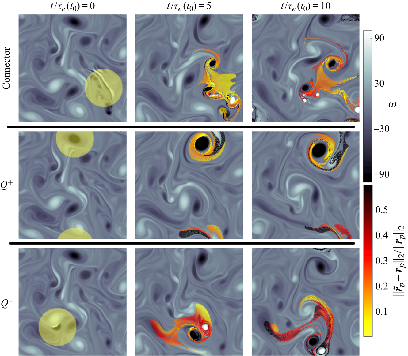
Figure 12. Time evolution of a two-dimensional isotropic turbulent flow subjected to multiple perturbations. Fluid tracers initialized around the perturbation are coloured by the change in trajectory with perturbation  $\tilde {\boldsymbol {r}}_p$ compared with the corresponding baseline trajectory
  $\boldsymbol {r}_p$.
Multiple pulses on the  $Q^{+}$ structure strengthens the vortex core, making a large distinct vortex. The tracers rotate around the vortex core due to the vorticity. Only the tracers at the boundary of the vortex are spread out significantly. The
  $Q^{-}$ perturbation, comprising the strained region between the vortex-dipoles, forms a jet-like flow. With multiple perturbations, the jet-like flow spreads the tracers more effectively compared with that achieved in the baseline and
  $Q^{+}$ perturbations. These observations are in agreement with recent findings that vortex-dipole-like structures in two-dimensional isotropic turbulence promote effective flow modification (Jiménez Reference Jiménez2020; Yeh et al. Reference Yeh, Gopalakrishnan Meena and Taira2021). The connector structures comprise a long shear-layer-type vortical structure and near-by vortices of low vorticity. Multiple perturbations of the shear-layer-type structure lead to the formation of small-scale vortices, which enhances flow mixing compared with the baseline, as well as
  $Q^{+}$ and
  $Q^{-}$ perturbations.
The evolution of particle tracers in a three-dimensional turbulent flow subjected to multiple perturbations on connector,  $Q^{+}$, and
  $Q^{-}$ structures are presented in figure 13. Here, the
  $Q^{+}$,
  $Q^{-}$ and connector structures are spatially located close to each other at the initial time instant. The flow field at the final instant corresponding to connector-based perturbation has the narrowest range in colour distribution of the tracers, depicting highest mixing enhancement. The broadest range in colour distribution corresponds to
  $Q^{+}$ perturbation, which denotes the least mixing enhancement achieved. Multiple pulses of connector-based perturbations lead to the generation of small-scale structures. On the other hand, the vortical structures decay in time with
  $Q^{+}$ and
  $Q^{-}$ perturbations.

Figure 13. Time evolution of a three-dimensional isotropic turbulent flow subjected to multiple perturbations. Vortical structures are depicted by isosurface of  $Q$-criterion. Fluid tracers initialized around the perturbation are coloured by the change in trajectory with perturbation
  $\tilde {\boldsymbol {r}}_p$ compared with the corresponding baseline trajectory
  $\boldsymbol {r}_p$.
Next, let us examine the local flow region around the perturbation to analyse the effect of the network-based connector to modify its neighbouring vortical structures. We analyse the time evolution of the local flow region around the connector,  $Q^{+}$, and
  $Q^{-}$ structures, as presented in figure 14. The vortical structures are tracked using the isosurface of
  $Q$-criterion, with a constant value of
  $Q$ in time. A single pulse is added to the connector,
  $Q^{+}$, and
  $Q^{-}$ structures at the initial time instant. The perturbed structures at the initial time instant are shown on the left column, visualized by the green isosurfaces. The neighbouring vortex tubes under consideration in each case (row) are depicted by the blue and red isosurface. The growth of maximum enstrophy,
  $\|\varOmega \|_\infty$, is also evaluated to observe modification of the vortex cores (Foias & Temam Reference Foias and Temam1989; Ayala & Protas Reference Ayala and Protas2017). We note that at time
 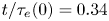 $t/\tau _e(0) = 0.34$, the connector structure leads to modification of both the neigboring vortex tubes and formation of smaller-scale structures. These small-scale structures induce enhanced local spreading of the fluid particles, as observed in figure 13.
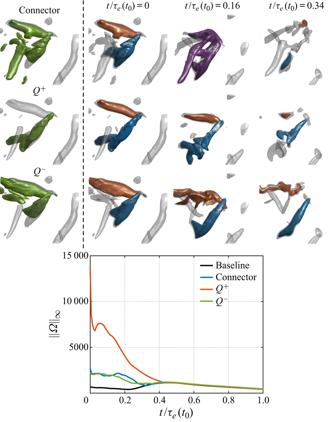
Figure 14. Modification of two vortex tubes in a three-dimensional isotropic turbulent flow using connector-based,  $Q^{+}$, and
  $Q^{-}$ perturbations. The vortical structures are visualized by the isosurface of
  $Q$-criterion, with a constant value of
  $Q$ in time. The green, blue and red colours of the isosurfaces represent the perturbed structures at the initial time and the two vortex tubes under consideration, respectively. The grey transparent isosurface denotes the background flow field for each case. The connector effectively modifies both the vortex cores as shown using the isosurface of
  $Q$-criterion and local growth of maximum enstrophy
  $\|\varOmega \|_\infty$ between time
  $t/\tau _e(0) = 0.12$ and
  $0.2$.
Perturbation of the  $Q^{+}$ structure (shown in blue) leads to the increase in circulation of the vortex core and eventual breakup of the blue isosurface at time
  $t/\tau _e(0) = 0.16$. The modification of the
  $Q^{+}$ structure is also observed by the peak of
  $\|\varOmega \|_\infty$ at
  $t/\tau _e(0) = 0.05$. The curved geometry of the
  $Q^{+}$ vortex core at the initial time instant may instigate instabilities when perturbation is added, resulting in the significant modification of the vortex core. Nonetheless, the
  $Q^{+}$ perturbation has negligible influence on the neighbouring vortex highlighted in red. Note that these observations are similar to the characteristics of a network-based peripheral structure. The
  $Q^{-}$ structure is the strongest shear-layer structure, which is located between the two neighbouring vortex tubes. Thus, the
  $Q^{-}$ perturbation results in the modification of both the blue and red isosurfaces. Both the vortex cores decay in time with no peaks appearing for
  $\|\varOmega \|_\infty$ over time, suggesting lower modification of the vortex cores achieved by the
  $Q^{-}$ structure compared with
  $Q^{+}$ perturbation.
The connector structure comprises the shear-layer region between the two neighbouring vortex tubes and an adjacent vortical structure with low circulation. This adjacent vortical structure merely decays within a short time in the  $Q^{+}$ and
  $Q^{-}$ simulations. With connector-based perturbation, the adjacent vortical structure connects with the two neighbouring vortex tubes through the shear layer, forming one large vortical structure highlighted in purple at time
  $t/\tau _e(0) = 0.16$. Eventually, the connection results in the significant breakup of both the blue and red isosurfaces, leading to the formation of smaller scales of vortical structures. The observations show the advantage of connectors to modify multiple vortical structures compared with
  $Q^{+}$ perturbations. The local growth of
  $\|\varOmega \|_\infty$ between
  $t/\tau _e(0) = 0.13$ and
  $0.2$ denotes effective modification of the vortex cores compared with that achieved by
  $Q^{-}$ perturbation. The connection amongst the vortical structures, in the form of vorticity, is not aligned with the direction of rotation of the two neighbouring vortex tubes, which may result in instabilities, leading to significant breakup of the vortex cores. The above illustrative examples demonstrate the ability of network-based methodologies to extract vortical structures of low circulation that can effectively influence neighbouring vortical structures in turbulent flows.
5. Concluding remarks
A network community-based formulation was introduced to extract flow-modifying vortical structures in two- and three-dimensional isotropic turbulence. The network framework considered the vortical elements in a flow as nodes of a vortical interaction network (graph). The web of interactions amongst the vortical elements was quantified by the induced velocity, which was assigned to the weighted network edges. This interaction-based framework was used to identify groups of closely connected vortical nodes, called communities. The interactions amongst these communities were used to identify the most influential community which can modify the system dynamics significantly. Taking advantage of the inter-community interactions, we showed that local turbulent mixing can be enhanced using vortical structures attributed with low circulation. The goal of this network-based framework was not to alter the global turbulent flow, but influence certain key vortical structures under the settings of isotropic turbulence.
We use the community characteristics to extract the inter- and intra-community interactions amongst groups of vortical nodes. The strengths of these interactions were used to identify the connector and peripheral nodes, which have the highest and least influence on other communities, respectively. The node with the maximum total interaction strength was identified as the hub. The ability of these influential nodes to modify the networked dynamics was demonstrated on a model fluid flow of a collection of discrete point vortices. Impulse velocity perturbations were added to the connector, peripheral and hub communities identified at the initial time instant. The connector community effectively modified trajectories of the other communities compared with the hub and peripheral-based perturbations. We then applied the community-based formulations to identify influential structures in two- and three-dimensional isotropic turbulence. The connector and peripheral structures were found to resemble shear-layer and vortex-core-type structures, respectively. Adding perturbations to the connector structures, which have low vorticity, led to enhanced local flow mixing compared with the effect of perturbing the strongest shear layer and vortex tube.
The present demonstrations of the network-based formulation on isotropic turbulence modification encourage the future extensions of the present framework on flows of practical interest. Within the current work, we have not considered the necessary computational effort for performing the network-based analysis. However, there are emerging network-based characterization (Bai et al. Reference Bai, Erichson, Gopalakrishnan Meena, Taira and Brunton2019) and modelling techniques (Nair & Taira Reference Nair and Taira2015) for fluid flows that can be leveraged to perform the present analysis with reduced computational resource. Moreover, the decomposition of the governing equation for a networked system using the inter- and intra-community interactions can be extended to community-based reduced-order modelling efforts for complex flows (Gopalakrishnan Meena et al. Reference Gopalakrishnan Meena, Nair and Taira2018). Based on these frameworks and extensions, the present characterization and open-loop control offers a pathway for future modelling and advanced flow control efforts to modify the dynamics of vortical structures in a complex turbulent flow field.
Acknowledgements
Some of the simulations were performed using the computational resource made available by the US Department of Defense High Performance Computing Modernization Program. We acknowledge thought-provoking discussions with Professors S.L. Brunton, J.C. McWilliams, Drs A.G. Nair and C.-A. Yeh.
Funding
The authors thank the US Army Research Office (Grants: W911NF-17-1-0118 and W911NF-19-1-0032, Program Manager: Dr M.J. Munson) for supporting this work.
Declaration of interests
The authors report no conflict of interest.
Appendix. Reynolds number and dimension reduction independence of network measures
We assess the effect of Reynolds number on the network representation of vortical interactions in isotropic turbulence by evaluating the node strength distribution for three-dimensional flow fields with various  $Re_\lambda$, as shown in figure 15(a). The strength distributions of flows with different Reynolds numbers collapse to a single curve with the use of appropriate non-dimensionalization for the edge weights. The results suggest that the network formulation is able to capture the key characteristics of the universal scaling of isotropic turbulence. The fine resolution of spatial discretization required to simulate turbulent flows also poses a challenge to analyse the interactions amongst the vortical elements. We subsample the flow field to reduce the dimension of the flow field being analysed.
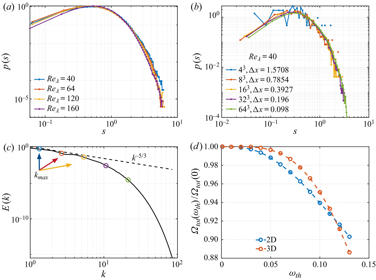
Figure 15. (a) Collapse of node strength distribution with increase in Reynolds number. (b) Convergence of node strength distribution over sampling rate in three-dimensional turbulence at  $Re_\lambda = 40$. (c) Maximum resolvable wavenumber for various grid resolution or sampling rate. (d) Variation of total enstrophy
  $\varOmega _{tot}$ with vorticity threshold for two- and three-dimensional turbulence.
The effect of subsampling the turbulent flow field on the network measures is evaluated by comparing the node strength distribution of various low-resolution flow fields. A three-dimensional flow field of  $Re_\lambda = 40$ with a grid resolution of
  $256\times 256\times 256$ is used. We subsample the data to various smaller grid resolutions and compute the node strengths, as shown in figure 15(b). The node strength computed based on the non-dimensionalized edge weight allows scaling of the distributions. The node strength distributions collapse into a single distribution and converge with higher grid resolution. The
  $k_{{max}}$ for each low-resolution grid used in the node strength distribution computation is depicted in the energy spectra in figure 15(c). The grid resolution using a
  $64\times 64\times 64$ grid satisfies the
  $k_{{max}} \eta \geqslant 1$ condition. The results also demonstrate the application of network-based formulation from a discrete to continuous description of the flow field.
We only analyse vortical elements in the flow field with high vorticity, extracted through vorticity threshold. The choice of the vorticity threshold of 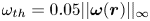 $\omega _{th}=0.05||\boldsymbol {\omega }(\boldsymbol {r})||_\infty$ is given by analysing the effect of thresholding on the total enstrophy of the flow field
  $\varOmega _{tot}$ (following (4.1)), as shown in figure 15(d). For both two- and three-dimensional turbulence,
  $\omega _{th}=0.05||\boldsymbol {\omega }(\boldsymbol {r})||_\infty$ results in retaining more than
  $98\,\%$ of the total enstrophy of the original flow field,
  $\varOmega _{tot}(\omega _{th}=0)$. This is similar to the values used to analyse structures of high vorticity (Jiménez et al. Reference Jiménez, Wray, Saffman and Rogallo1993; Moisy & Jiménez Reference Moisy and Jiménez2004), capturing the influential regions of the flow.


 Open access