3.1. Detection of the TNTI layer

Following previous studies (da Silva et al. Reference da Silva, Hunt, Eames and Westerweel2014), an isosurface of vorticity magnitude $\omega =\omega _{th}$ is used to detect the outer edge of the TNTI layer, which is called the irrotational boundary (Watanabe et al. Reference Watanabe, Sakai, Nagata, Ito and Hayase2015). Obviously, the location of the isosurface changes with the threshold value $\omega _{th}$. In this method, a fluid point with $\omega >\omega _{th}$ is denoted as a turbulent fluid point, while a non-turbulent fluid point has $\omega <\omega _{th}$. For determining an appropriate value of $\omega _{th}$ for studying the TNTI layer, the volume of the turbulent region $V_T$ is computed as a function of $\omega _{th}$, as shown in figure 3. The threshold $\omega _{th}$ shown in the figure is normalized as $\hat {\omega }_{th}=\omega _{th}/\langle \omega \rangle _c$, where the subscript $c$ denotes the value taken at $y=0.5\delta$, which is located in the turbulent core region. The volume of the turbulent region is also normalized, as $\hat {V}_T=V_T/(L_xL_z\delta )$. Figure 3 also shows the derivative of $\hat {V}_T$, ${\rm d}\hat {V}_T/{\rm d}\log (\hat {\omega }_{th})$. The profile of $\hat {V}_T$ is similar to profiles obtained in previous studies (da Silva et al. Reference da Silva, Hunt, Eames and Westerweel2014; Jahanbakhshi, Vaghefi & Madnia Reference Jahanbakhshi, Vaghefi and Madnia2015; Watanabe et al. Reference Watanabe, Sakai, Nagata, Ito and Hayase2015). The turbulent volume largely increases for $\hat {\omega }_{th}<10^{-4}$ as $\hat {\omega }_{th}$ decreases, because the non-turbulent region has very small vorticity magnitude, which is often associated with the numerical error. On the other hand, $\hat {V}_T$ hardly changes within the range $10^{-3} < \hat {\omega }_{th} < 10^{-2}$, which indicates that the location of the isosurface $\omega =\omega _{th}$ hardly changes with $\omega _{th}$ within this range. In the present study, $\hat {\omega }_{th}=10^{-2.5}$ shown as a vertical dot-dash line in figure 3 is used to detect the irrotational boundary.

Figure 3. The normalized turbulent volume $\hat {V}_T$ plotted against the normalized threshold $\hat {\omega }_{th}$ used for detecting turbulent fluids. Here, ${\rm d}\hat {V}_T/{\rm d}\log (\hat {\omega }_{th})$ is also plotted, with dashed lines. A vertical dot-dash line indicates the threshold value used in this study to detect the irrotational boundary.

This method based on the threshold dependence of the turbulent volume has been used widely for choosing the isosurface value for studying the TNTI layer (Taveira et al. Reference Taveira, Diogo, Lopes and da Silva2013; Jahanbakhshi et al. Reference Jahanbakhshi, Vaghefi and Madnia2015). Statistics near the TNTI layer are often computed as functions of the distance from the isosurface $\omega =\omega _{th}$ (Bisset et al. Reference Bisset, Hunt and Rogers2002). Previous studies have shown that the statistics near the TNTI layer hardly change with a small change of $\omega _{th}$ if $\omega _{th}$ is chosen based on the $\omega _{th}$ dependence of the turbulent volume (Taveira et al. Reference Taveira, Diogo, Lopes and da Silva2013; Watanabe et al. Reference Watanabe, Zhang and Nagata2018b; Watanabe, da Silva & Nagata Reference Watanabe, da Silva and Nagata2019a). We have also tested different values of $\omega _{th}$ within the range $10^{-3}<\hat {\omega }_{th}<10^{-2}$ with the present DNS database, and have found that the detected isosurface location and the statistics near the TNTI layer are insensitive to the threshold.

Figure 4 visualizes the irrotational boundary coloured by the height of the irrotational boundary from the wall, $y_{IB}$, for $Re_{\theta }=2000$ and $13\,000$. The irrotational boundary in the present DNS looks very smooth and similar to those detected in free shear flows (Watanabe, Riley & Nagata Reference Watanabe, Riley and Nagata2017b; Nagata et al. Reference Nagata, Watanabe and Nagata2018), while some previous DNS of the TBL with coarser grids ($\varDelta _x^{+}\approx 9$) showed spiky patterns of the irrotational boundary, as discussed in Zhang et al. (Reference Zhang, Watanabe and Nagata2018) and Watanabe et al. (Reference Watanabe, Zhang and Nagata2018b). A folded shape of the irrotational boundary can be characterized by a wide range of length scales of turbulent motions that appear under the TNTI layer. Therefore, the small-scale structures appear in $Re_{\theta }=13\,000$ rather than in $Re_{\theta }=2000$. Figure 5 shows a colour contour of enstrophy $\omega ^{2}/2$ and the irrotational boundary on an $x$–$y$ plane. The geometries of the irrotational boundary are different for $Re_{\theta }=2000$ and 13 000, where the irrotational boundary is more folded for higher $Re_{\theta }$, but flatter for lower $Re_{\theta }$. The mean height of the irrotational boundary is approximately $0.9\delta$ for all the Reynolds numbers, and the irrotational boundary appears for $0.4\delta \leq y \leq 1.4\delta$, which is consistent with an intermittency factor profile in spatially developing TBLs (Borrell & Jiménez Reference Borrell and Jiménez2016).

Figure 4. Visualization of an irrotational boundary forming at the outer edge of the TNTI layer for (a) case B02 ($Re_\theta = 2000$), and (b) case B13 ($Re_\theta = 13\,000$). Colour represents the height of irrotational boundary $y_{IB}$.

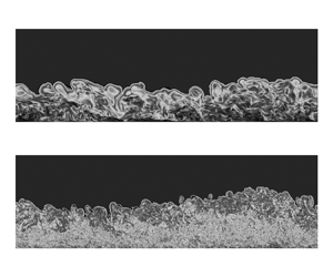
Figure 5. Two-dimensional snapshots of temporally developing boundary layers on the $x$–$y$ plane. The colour represents vorticity magnitude $\log (\omega D/U_W)$, and the irrotational boundary is visualized with the white line. The wall is moving in the $x$ direction (from left to right): (a) case B02 ($Re_\theta = 2000$), (b) case B13 ($Re_\theta = 13\,000$).

The TNTI layer can be studied with statistics conditioned on the distance from the irrotational boundary. The local coordinate $y_I$ is defined so that the irrotational boundary is located at $y_I = 0$, and the direction of $y_I$ is normal to the irrotational boundary, pointing into the non-turbulent region. Here, the normal direction of the irrotational boundary can be obtained as $\boldsymbol {n} = -\boldsymbol {\nabla }\omega ^2/|\boldsymbol {\nabla }\omega ^2|$, and the non-turbulent and turbulent regions are represented by $y_I>0$ and $y_I<0$, respectively. The conditional statistics are obtained as functions of $y_I$, where samples of the statistics for $y_I>0$ and $y_I<0$ are taken only from non-turbulent and turbulent flow points, respectively, even though the local coordinate $y_{I}$ intersects more than one irrotational boundary point. Further details of the computation of the conditional statistics can be found in our previous papers (Nagata et al. Reference Nagata, Watanabe and Nagata2018; Watanabe et al. Reference Watanabe, Zhang and Nagata2018b, Reference Watanabe, da Silva and Nagata2019a; Zhang et al. Reference Zhang, Watanabe and Nagata2018). The average taken on the local coordinate is denoted by $\langle \cdot \rangle _{I}$.

3.2. Mean thickness of the TNTI layer and sublayers

The TNTI layer can be defined as a region where the vorticity magnitude is adjusted between the turbulent and non-turbulent regions (da Silva et al. Reference da Silva, Hunt, Eames and Westerweel2014). Therefore, the TNTI layer can be characterized by a large gradient of vorticity magnitude in the TNTI normal direction. The mean thickness of the TNTI layer is quantified based on the mean vorticity magnitude $\langle \omega \rangle _I$, as shown in figure 6(a) following our previous studies (Watanabe et al. Reference Watanabe, Riley, Nagata, Onishi and Matsuda2018a; Zhang et al. Reference Zhang, Watanabe and Nagata2018). Figure 6(a) also shows the derivative of $\langle \omega \rangle _I$, $\langle \omega \rangle '_I = -{\rm d}\langle \omega \rangle _I /{\rm d}y_I$, where the mean thickness of the TNTI layer, $\delta _{TNTI}$, is defined as the distance from $y_{I}=0$ to the location where $\langle \omega \rangle '_I$ reaches 20 % of its maximum value. The mean thickness of the TNTI layer was also quantified by fitting an error function to the conditional statistics in the previous study, and both methods result in a similar value of the mean thickness of the TNTI layer (Watanabe et al. Reference Watanabe, Riley, Nagata, Onishi and Matsuda2018a).

Figure 6. (a) Conditional mean vorticity and its derivative with respect to $y_I$ for case B02. (b) Conditional profiles of Kolmogorov length scale $\eta _I$ and Taylor microscale $\lambda _I$ defined with conditional averages. The line colours represent the Reynolds numbers as shown in figure 3. The vertical dot-dash line shows $y_I/\delta _{TNTI}=-2$, where the reference scales are taken for studying the TNTI layer.

Figure 6(b) shows the conditional profiles of Kolmogorov scale defined as $\eta _I =\nu ^{3/4} \langle \varepsilon \rangle _{I}^{-1/4}$ and Taylor microscale defined as $\lambda _I=\sqrt {10k_{I}/(\langle \varepsilon \rangle _{I} \nu )}$, where $k_{I}$ is the turbulent kinetic energy defined as $k_{I} = (\langle u_i^2 \rangle _{I} - \langle u_i \rangle _{I}^2)/2$. The distance from the irrotational boundary, $y_I$, is normalized by $\delta _{TNTI}$. These two scales are quite large in the non-turbulent region, then decrease rapidly from the non-turbulent region to the turbulent region, and tend to be constant in the turbulent core region. The turbulent statistics at $y_I/\delta _{TNTI}=-2$ shown by the vertical dot-dash line are used as reference quantities for investigating the TNTI layer. The choice $y_I/\delta _{TNTI}=-2$ ensures the ‘same’ distance from the TNTI layer for different Reynolds numbers. Hereafter, the subscript ‘$TI$’ indicates the statistics taken at this location. The corresponding turbulent Reynolds number $Re_{\lambda.TI}=\lambda _{TI} \sqrt {(2/3)k_{TI}}/\nu$ near the TNTI layer at $y_I/\delta _{TNTI}=-2$ is also calculated, and shown in table 3.

Table 3. Turbulent Reynolds number $Re_{\lambda.TI}$ of the turbulent flow near the TNTI layer at $y_I/\delta _{TNTI}=-2$.

The TNTI layer contains two sublayers, the viscous superlayer (VSL) and the turbulent sublayer (TSL). These inner structures of the TNTI layer can be distinguished by vorticity dynamics (van Reeuwijk & Holzner Reference van Reeuwijk and Holzner2014; Taveira & da Silva Reference Taveira and da Silva2014). The conditional averages of the production term $\langle P_\omega \rangle _{I}$ and the viscous diffusion term $\langle D_\omega \rangle _{I}$ in the enstrophy transport equation can be used for identifying the VSL and TSL (Taveira & da Silva Reference Taveira and da Silva2014; Zhang et al. Reference Zhang, Watanabe and Nagata2018). The enstrophy transport equation is

(3.1)\begin{equation} \frac{{\rm D}(\omega^2/2) }{{\rm D}t} = \omega_i {\mathsf{S}}_{ij} \omega_j + \nu\, \nabla^2 (\omega^2/2) + \nu\,\boldsymbol{\nabla} \omega_i \boldsymbol{\cdot} \boldsymbol{\nabla} \omega_i. \end{equation}

The three terms on the right-hand side are the production $\langle P_\omega \rangle _{I}$, viscous diffusion $\langle D_\omega \rangle _{I}$ and viscous dissipation $\langle \varepsilon _\omega \rangle _{I}$, respectively. The production term $\langle P_\omega \rangle _{I}$ and the viscous diffusion term $\langle D_\omega \rangle _{I}$ are almost 0 at the irrotational boundary ($y_I=0$), then they increase from the irrotational boundary towards the turbulent region. The mean viscous diffusion term is larger than the production term near the irrotational boundary, where the mean thickness of the VSL, $\delta _{VSL}$, can be identified as the region where $\langle D_\omega \rangle _{I} > \langle P_\omega \rangle _{I}$ near the irrotational boundary (Taveira & da Silva Reference Taveira and da Silva2014; Jahanbakhshi et al. Reference Jahanbakhshi, Vaghefi and Madnia2015; Watanabe et al. Reference Watanabe, Sakai, Nagata, Ito and Hayase2015; Zhang et al. Reference Zhang, Watanabe and Nagata2018). Then it is easy to measure the mean thickness of the TSL, $\delta _{TSL}$, which is considered as the buffer region between the VSL and the turbulent core region. Within the TSL, the inviscid process (production term) has a larger contribution to the increase of the enstrophy (da Silva et al. Reference da Silva, Hunt, Eames and Westerweel2014). The mean thicknesses of the TNTI layer ($\delta _{TNTI}$), VSL ($\delta _{VSL}$) and TSL ($\delta _{TSL}$) normalized by Kolmogorov scale $\eta _{TI}$ and Taylor microscale $\lambda _{TI}$ near the TNTI layer are plotted in figures 7(a) and 7(b), respectively. From figure 7(a), we can see that the average thickness of $\delta _{TNTI}$ is approximately 15.7$\eta _{TI}$, $\delta _{VSL}$ is approximately 4.6$\eta _{TI}$, and $\delta _{TSL}$ is approximately 11.1$\eta _{TI}$ for all the Reynolds numbers. However, $\delta _{TNTI}/\lambda _{TI}$, $\delta _{TSL}/\lambda _{TI}$ and $\delta _{VSL}/\lambda _{TI}$ all decrease with the increase of the Reynolds number, as shown in figure 7(b). These results are consistent with a previous study (Silva et al. Reference Silva, Zecchetto and da Silva2018), in which the thickness of the TNTI layer and sublayers normalized by the Kolmogorov scale is almost constant for the different Reynolds numbers, while the thickness normalized by $\lambda$ decreases with $Re_\lambda ^{-1/2}$ in jets and shear-free turbulence. Hereafter, we assume that the mean thicknesses of the TNTI layer and VSL are approximately $15\eta _{TI}$ and $5\eta _{TI}$, for convenience. Our result is also consistent with the results from Jahanbakhshi (Reference Jahanbakhshi2021), where $\delta _{VSL}$ is approximately $5\eta$, and $\delta _{TNTI}$ is of the order of $O(10\eta )$ at $Re_\tau \approx 600$ in the spatial TBL.

Figure 7. The mean thickness of the TNTI layer, the viscous superlayer (VSL), and the turbulent sublayer (TSL) normalized by (a) Kolmogorov scale $\eta _{TI}$, and (b) Taylor microscale $\lambda _{TI}$, at $y_I/\delta _{TNTI}=-2$.

3.3. The turbulent statistics near and within the TNTI layer

Figure 8(a) shows the conditional mean vorticity magnitude $\langle \omega \rangle _I$ normalized by wall velocity $U_W$ and trip wire diameter $D$ with $y_I$ normalized by $\eta _{TI}$. The mean vorticity magnitude in figure 8(a) decreases with the increase of Reynolds number. In the meantime, the vertical profiles of the average of $\omega$ taken only from the turbulent region, $\langle \omega \rangle _T$, in comparison with the conventional average $\langle \omega \rangle$, are shown in figure 8(b). Because turbulent fluids have $\omega \geq \omega _{th}$, $\langle \omega \rangle _T$ does not decrease to 0 for large $y$, unlike $\langle \omega \rangle$, which decreases to 0 for large $y$. In the figure, the location of the mean irrotational boundary height is marked by circles. In the intermittent region, where $\langle \omega \rangle$ differs from $\langle \omega \rangle _T$, $\langle \omega \rangle _T$ tends to be independent of large $y^+$ at high Reynolds numbers. On the other hand, $\langle \omega \rangle _T$ in the intermittent region still rapidly decreases with $y^+$ for low Reynolds numbers. This strong dependence of $\langle \omega \rangle _T$ on $y^+$ can be seen near the wall for all Reynolds numbers. Since the ratio between $y$ and $\delta _\nu$ is small in the intermittent region at a low Reynolds number, the intermittent region can be influenced by the wall, and $\langle \omega \rangle _T$ in the intermittent region depends strongly on $y$. On the other hand, because $y/\delta _\nu$ in the intermittent region is large at high Reynolds numbers, the intermittent region in this case is less influenced by the strong mean shear near the wall. This results in the weak dependence of $\langle \omega \rangle _T$ on $y$ in the intermittent region.

Figure 8. (a) Conditional mean profile of vorticity magnitude normalized by wall velocity $U_W$ and trip wire diameter $D$ plotted with respect to $y_I/\eta _{TI}$. (b) Vertical profiles of the mean vorticity magnitude computed only from turbulent fluids, $\langle \omega \rangle _T$, and the conventional average of $\omega$ based on the spatial average on $x$–$z$ planes, $\langle \omega \rangle$. The circle symbols represent the mean irrotational boundary height, and the inset shows $\langle \omega \rangle$, $\langle \omega \rangle _T$ normalized by the boundary layer thickness $\delta$. The line colours represent the Reynolds numbers as shown in figure 3.

Figure 9(a) shows $\langle \omega \rangle _I$ normalized by vorticity $\omega _{TI}$ at $y_I=-2\delta _{TNTI}$. The mean vorticity jump at different Reynolds numbers collapses well within the TNTI layer ($y_I$ from 0 to approximately 15$\eta _{TI}$) in figure 9(a). The conditional averages of second invariant of velocity gradient tensor $\langle Q \rangle _I$ are plotted in figure 9(b). Here, $Q$ is defined as $Q=(\boldsymbol{\mathsf{\omega _{ij}}} \boldsymbol{\mathsf{\omega _{ij}}}-{\mathsf{S}}_{ij}{\mathsf{S}}_{ij})/2$, with $\boldsymbol{\mathsf{\omega _{ij}}} =({\partial u_i }/{\partial x_j}-{\partial u_j }/{\partial x_i})/2$ and ${\mathsf{S}}_{ij}=({\partial u_j }/{\partial x_i}+{\partial u_i }/{\partial x_j})/2$. We also normalize $\langle Q\rangle _I$ by the mean strain product taken at $y_I=-2\delta _{TNTI}$, which is denoted as $s^2_{TI}$. In this figure, the profiles for different Reynolds numbers also collapse together. In these profiles, we can see that the vorticity is weaker than strain ($Q<0$) within the VSL, and stronger than strain ($Q>0$) within the TSL, as also found in other free shear flows. Here, figures 9(a) and 9(b) both indicate that the turbulent characteristics taken at $y_I=-2\delta _{TNTI}$ well characterize the statistics near the TNTI layer. The DNS results for a temporally developing planar jet with jet Reynolds number 10 000 (Watanabe et al. Reference Watanabe, Zhang and Nagata2019b) are also compared in figure 9. The shape and magnitude of the conditional mean vorticity and the second invariant of velocity gradient tensor are similar between the jet and TBL when they are normalized by $\eta _{TI}$.

Figure 9. The normalized conditional mean profiles of (a) mean vorticity magnitude $\langle \omega \rangle _I / \omega _{TI}$, and (b) the second invariant of velocity gradient tensor $\langle Q \rangle _I / s^2_{TI}$, where $\omega _{TI}$ and $s^2_{TI}$ represent $\langle \omega \rangle _I$ and $\langle {\mathsf{S}}_{ij}{\mathsf{S}}_{ij}\rangle _I$ calculated at $y_I/\delta _{TNTI}=-2$, respectively. The line colours represent the Reynolds numbers as shown in figure 3. The circle symbols represent the data of a turbulent planar jet with the jet Reynolds number $10\,000$ (Watanabe et al. Reference Watanabe, Zhang and Nagata2019b).

Figure 10(a) shows the conditional mean streamwise velocity $\langle u \rangle _I$ normalized by the friction velocity $u_\tau$. The conditional mean velocity is very small and almost constant within the VSL, then it increases rapidly in the TSL, and the mean velocity is still increasing gradually in the turbulent core region. However, the mean streamwise velocity is flat within the VSL, which indicates that the mean shear is absent within the VSL. In this study, $\langle u \rangle _I$ is qualitatively different from the result by Eisma et al. (Reference Eisma, Westerweel, Ooms and Elsinga2015), which is well approximated by their Z-shape model. The Z-shape model is characterized by sudden changes of the mean velocity gradient at the boundaries among the turbulent core region, the TNTI layer and the non-turbulent region. The present results confirm that $\langle u \rangle _I$ increases from the TNTI layer to the turbulent core region without a significant change of the mean velocity gradient. It seems that this difference is due to different definitions of the local coordinate used for the conditional statistics. Eisma et al. (Reference Eisma, Westerweel, Ooms and Elsinga2015) considered the local coordinate taken in the wall-normal direction, while $y_I$ in this study is taken in the interface normal direction. It was also shown that the Z-shape model for $\langle u \rangle _I$ is valid in a turbulent planar jet if the local coordinate is taken in the transverse direction of the jet (Watanabe et al. Reference Watanabe, Sakai, Nagata, Ito and Hayase2014). These results indicate that the conditional mean velocity profile near the TNTI layer is sensitive to the definition of the local interface coordinate. The inset of figure 10(a) shows $\langle u \rangle _I$ normalized by $u_{rms.TI}$, which is the r.m.s. of streamwise velocity $u_{rmsI}$ at $y_I/\delta _{TNTI}=-2$. Here, $u_{rmsI}$ is defined as $\sqrt { \langle u^2 \rangle _I - \langle u \rangle _I^2 }$. The velocity jump of $\langle u \rangle _I$ across the TNTI layer is approximately one order of $u_{rms.TI}$. The temporally developing planar jet with jet Reynolds number 10 000 (Watanabe et al. Reference Watanabe, Zhang and Nagata2019b) is also compared in figure 10(a), where the profiles are similar for the jet and TBL when $y_I$ is normalized by $\eta _{TI}$. Even though it seems from figure 10(a) that the mean shear exists within and near the TNTI layer, how significantly the mean shear affects the TNTI layer is still not clear.

Figure 10. (a) Conditional mean streamwise velocity $\langle u \rangle _I$ and (b) conditional mean vertical velocity $\langle v \rangle _I$, normalized by the friction velocity $u_\tau$. The inset in (a) shows $\langle u \rangle _I$ normalized by the r.m.s. streamwise velocity fluctuation $u_{rms.TI}$ calculated at $y_I/\delta _{TNTI}=-2$. The circle symbols represent the data of a turbulent planar jet with jet Reynolds number $10\,000$ (Watanabe et al. Reference Watanabe, Zhang and Nagata2019b).

Figure 10(b) shows the conditional mean of vertical velocity, $\langle v \rangle _I / u_\tau$, which becomes positive in the turbulent core region and negative in the non-turbulent region. This profile is consistent with previous studies on a spatially developing TBL (Eisma et al. Reference Eisma, Westerweel, Ooms and Elsinga2015) and a turbulent planar jet (Watanabe et al. Reference Watanabe, Sakai, Nagata, Ito and Hayase2014). Negative $\langle v \rangle _I / u_\tau$ in the non-turbulent region is expected from large-scale motions, such as sweeps (Pope Reference Pope2000) in TBLs, which are expected to be related to the engulfment. The engulfment process can draw the non-turbulent fluids towards the turbulent region directly, where the valley structures appear on the TNTI with the negative $\langle v \rangle _I$ in the non-turbulent region. The profile of $\langle v \rangle _I$ is also consistent with experimental results obtained for the interface detected with kinetic energy (Chauhan et al. Reference Chauhan, Philip and Marusic2014a; de Silva et al. Reference de Silva, Philip, Hutchins and Marusic2017). The mean vertical velocity defined with an average taken on a horizontal plane, $\langle v\rangle$, is zero at any locations in the temporally developing TBLs, unlike in spatially developing TBLs. However, the conditional profile of $\langle v \rangle _I$ is consistent between temporal and spatial TBLs, and the non-turbulent fluid motions in the vicinity of the interface are similar in both temporal and spatial TBLs. These non-turbulent fluid motions are related to a part of the entrainment process, and the temporal simulation well captures the process by which the non-turbulent fluid is transferred towards the TNTI in the intermittent region of spatially developing TBLs. Also, the changes in the conditional mean streamwise and vertical velocities across the TNTI layer are of the same order as in previous studies (Chauhan et al. Reference Chauhan, Philip and Marusic2014a; Eisma et al. Reference Eisma, Westerweel, Ooms and Elsinga2015).

The conditional r.m.s. values of streamwise velocity $u_{rmsI}$, wall-normal velocity $v_{rmsI}$ and spanwise velocity $w_{rmsI}$ are shown in figure 11. It should be noticed again that the conditional r.m.s. of streamwise velocity $u_{rmsI}$ is defined as $\sqrt { \langle u^2 \rangle _I - \langle u \rangle _I^2 }$; $v_{rmsI}$ and $w_{rmsI}$ are calculated in the same way as $u_{rmsI}$. The low Reynolds number case has a larger r.m.s. value for all velocity components in the turbulent region, but the r.m.s. velocity fluctuations tend to be independent of the Reynolds number for high Reynolds numbers. This might be because the production term of the turbulent kinetic energy budget is almost 0 for large $y^+$ (Smits, McKeon & Marusic Reference Smits, McKeon and Marusic2011). As we mentioned before, the height $y_{IB}$ of the irrotational boundary is approximately $0.9\delta$, namely $y_{IB}^+ \approx 0.9 Re_{\tau }$, which is why the r.m.s. fluctuations of the three velocity components are similar to each other for high Reynolds numbers. The jumps of r.m.s. velocity fluctuations near the TNTI layer in the present DNS are of the same order in their experimental results (Chauhan et al. Reference Chauhan, Philip and Marusic2014a), where the TBLs are investigated experimentally between $Re_{\tau }=1230$ and $Re_{\tau }=14\,500$.

Figure 11. Conditional r.m.s. velocity fluctuations: (a) streamwise velocity, (b) wall-normal velocity, and (c) spanwise velocity. The line colours represent the Reynolds numbers as shown in figure 3.

3.4. The shear effects near and within the TNTI layer

As shown in figure 10, the mean shear exists within and near the TNTI layer, where we investigate how significantly the mean shear affects the TNTI layer. Therefore, the conditional shear parameter defined as $S^*_I = \langle \partial u / \partial y \rangle _I \langle k \rangle _I / \langle \varepsilon \rangle _I$ based on the conditional mean streamwise velocity derivative is calculated for evaluating the shear effects on the energy-containing eddies near the TNTI. The shear parameter is defined as the ratio between the decay time of energy-containing eddies and the shear deformation time (Corrsin Reference Corrsin1958). Figure 12(a) shows that the conditional shear parameter is approximately 4 in the turbulent core region for all the Reynolds numbers, and the value of $S^*_I$ is within the typical range (from 3 to 6) in turbulent shear flows (Pope Reference Pope2000). The conditional shear parameter decreases from the TSL towards the irrotational boundary ($y_I$ from 15 to 0). The value of the shear parameter indicates that the shear effects do exist near and within the TNTI layer, but are not very significant on the large-scale eddies. Furthermore, the value of the shear parameter within the TNTI layer is in the typical range of shear flows (Pope Reference Pope2000).

Figure 12. (a) Conditional shear parameter defined as $S^*_I = \langle \partial u / \partial y \rangle _I \langle k \rangle _I / \langle \varepsilon \rangle _I$ near the TNTI layer. (b) Conditional shear-to-vorticity ratio $S_I/\omega '_I$ near the TNTI layer. The line colours represent the Reynolds numbers as shown in figure 3.

The conditional shear-to-vorticity ratio $S_I/\omega _I'$ is shown in figure 12(b), where the conditional mean shear $S_I$ is defined as $S_I = \langle \partial u / \partial y \rangle _I$, and the conditional fluctuation $\omega _I'$ is defined as $\omega _I'= \sqrt {\langle \omega _I^2 \rangle - \langle \omega _I \rangle ^2}$. This ratio indicates the relative shear effects on the small-scale motions near the TNTI. If $S_I/\omega _I'$ is much smaller than 1, then the small-scale vortices are decoupled from the mean shear and become roughly isotropic (Jiménez Reference Jiménez2013). As shown in figure 12(b), $S_I/\omega _I'$ under the TNTI layer is approximately $0.1$–$0.2$. These values are so small that the mean shear effects on small-scale motions are weak. The Reynolds number dependence can still be found in this figure: the results with a higher Reynolds number have a lower value of $S_I/\omega _I'$, which means that the vortices tend to be more isotropic with the increase of Reynolds number. This observation is similar to that found by computing conventional average $S/\omega '$ in the outer layer ($y=0.6\delta$) (Jiménez Reference Jiménez2013). Finally, because the irrotational boundary ($y_I=0$) is detected by a vorticity magnitude isosurface, the vorticity fluctuation is close to zero near the irrotational boundary, which causes the large value of $S_I/\omega _I'$ near the irrotational boundary.

In general, the boundary layer thickness $\delta$ represents the characteristic length scale of large-scale motions (Pope Reference Pope2000), and $\eta _{TI}$ indicates the smallest scale of the turbulence near the TNTI layer. Figure 13(a) shows the ratio between $\eta _{TI}$ and $\delta$ against the Reynolds number $Re_{\theta }$. The red dot-dash line represents $C_1\,Re_\theta ^{-3/4}$, where $C_1=2.3$ is a constant obtained from the present DNS data with $Re_{\theta }\geq 4000$. It is a scaling law for homogeneous isotropic turbulence (HIT), $\eta /l_0 \sim Re^{-3/4}$, where $l_0$ is the integral length scale that represents the length scale of large-scale motions for homogeneous isotropic turbulence (Pope Reference Pope2000). It can be seen clearly that the results at relatively high Reynolds numbers ($Re_{\theta }=6000$–$13\,000$) agree well with the red dot-dash line. However, the results for $Re_{\theta }=2000$ and $4000$ are lower than this line, especially for $Re_{\theta }=2000$. It is expected that the wall has more significant influences on the TNTI layer at lower Reynolds numbers, which might explain the departure from $\eta /\delta \sim Re_\theta ^{-3/4}$.

Figure 13. (a) The $Re_{\theta }$ dependence of the length scale ratio between the Kolmogorov scale $\eta _{TI}$ and boundary layer thickness $\delta$ at $y_I/\delta _{TNTI}=-2$. The inset shows the corresponding plot with a linear scale. (b) The second invariants of the anisotropy tensor of Reynolds stress and vorticity for turbulence near the TNTI, which are denoted $B2_{TI}$ and $V2_{TI}$, respectively.

Figure 13(b) shows the second invariants of the anisotropy tensors of the Reynolds stress and vorticity in the turbulent region near the TNTI, $B2_{TI}$ and $V2_{TI}$. These invariants are defined as $B2_{TI}=(3 \langle {\mathsf{b}}_{ij}\rangle _{TI} \langle {\mathsf{b}}_{ij} \rangle _{TI} /2)^{1/2}$ and $V2_{TI}=(3 \langle {\mathsf{v}}_{ij}\rangle _{TI} \langle {\mathsf{v}}_{ij} \rangle _{TI}/2)^{1/2}$, respectively, with the anisotropy tensors of the Reynolds stress and vorticity:

(3.2)\begin{gather} \langle {\mathsf{b}}_{ij} \rangle_{TI} =\frac{ \langle u_{i}u_{j} \rangle_{TI} - \langle u_{i}\rangle_{TI} \langle u_{j}\rangle_{TI} } {\langle u_{k} u_{k} \rangle_{TI} - \langle u_{k}\rangle_{TI} \langle u_{k}\rangle_{TI} }-\frac{1}{3}\,\boldsymbol{\mathsf{\delta_{ij}}}, \end{gather}

(3.3)\begin{gather}\langle {\mathsf{v}}_{ij} \rangle_{TI} =\frac{\langle \omega_{i}\omega_{j} \rangle_{TI}}{\langle \omega_{k}\omega_{k} \rangle_{TI}}-\frac{1}{3}\,\boldsymbol{\mathsf{\delta_{ij}}}. \end{gather}

Here, $\delta _{ij}$ is Kronecker's delta. The values of $B2_{TI}$ and $V2_{TI}$ indicate the anisotropy related to the large- and small-scale turbulent motions under the TNTI, respectively. The invariants are equal to 1 and 0 for complete anisotropy and isotropy, respectively. In the figure, $B2_{TI}$ is larger than $V2_{TI}$, indicating that large-scale motions are more anisotropic compared with small-scale ones. Higher isotropy for smaller scales is related to the weak mean shear effects for small-scale motions as examined with $S_I/\omega _I'$ in figure 12(b). As expected from the above discussion, both invariants decrease with the Reynolds number, and the flow under the TNTI becomes close to isotropic turbulence. This behaviour is related to the departure from the scaling law for HIT at the low Reynolds numbers as shown in figure 13(a). A similar observation was made by Jiménez (Reference Jiménez2013), where the turbulence motions in the outer layer become more isotropic with the increase of Reynolds number in channel flow.

3.5. The geometry of the irrotational boundary

The probability density function (p.d.f.) of the mean curvature $H = (1/2) \boldsymbol {\nabla }\boldsymbol {\cdot }\boldsymbol {n}$ of the irrotational boundary is shown in figure 14, where the p.d.f. is normalized by the Kolmogorov length scale $\eta _{TI}$ in figure 14(a), and by the Taylor microscale $\lambda _{TI}$ in figure 14(b). The positive/negative value of $H$ indicates the concave/convex region in the top view of the TBL shown in figure 4. The profiles of p.d.f.s normalized by $\eta _{TI}$ are similar with different Reynolds numbers ($Re_{\theta }=2000$–$13\,000$); in particular, the locations and values of peaks in the p.d.f.s collapse together for all the Reynolds numbers. The p.d.f. normalized by $\lambda _{TI}$ depends strongly on the Reynolds number, as confirmed by the variation of the peak value and location of the p.d.f. with the Reynolds number. Therefore, the mean curvature of the irrotational boundary is well characterized by the Kolmogorov scale $\eta _{TI}$. The DNS results for a temporally developing planar jet with jet Reynolds number 10 000, ($Re_\lambda =97$) (Watanabe et al. Reference Watanabe, Zhang and Nagata2019b) are also compared in figure 14(a). The p.d.f. of the mean curvature hardly differs for the jet and TBL when they are normalized by $\eta _{TI}$. The p.d.f. has a peak at $H \eta _{TI}\approx -0.025$, which indicates that a large part of the irrotational boundary has curvature radius approximately $40\eta _{TI}$. The length $40\eta _{TI}$ is the typical length scale of velocity gradients in the outer logarithmic layer or outer layer (Jiménez Reference Jiménez2013). On the other hand, the mean curvature p.d.f. normalized by $\lambda _{TI}$ for the jet ($Re_\lambda =97$) collapses with $Re_\theta =10\,000$ ($Re_{\lambda.TI}=90$) for the TBL but differs for lower Reynolds numbers, which also indicates that the p.d.f. normalized by $\lambda _{TI}$ depends on the Reynolds number. With flow visualization, previous studies observed small-scale vortex tubes within the TNTI layer, and the interface forms around them (da Silva, Dos Reis & Pereira Reference da Silva, Dos Reis and Pereira2011). The curvature of the TNTI is expected to be related to the diameter of the vortices or the curvature radius of the vortex axis since both the curvature radius of the TNTI and the length scale of vortex tubes scale with the Kolmogorov scale. This is geometrical information about the irrotational boundary, which is expected to be related to the turbulent structure with a similar length scale beneath the irrotational boundary.

Figure 14. The p.d.f.s of the mean curvature of the irrotational boundary normalized by (a) Kolmogorov length scale $\eta _{TI}$, and (b) Taylor microscale $\lambda _{TI}$. The line colours represent the Reynolds numbers as shown in figure 3. The circle symbols represent the data of a turbulent planar jet with jet Reynolds number $10\,000$ (Watanabe et al. Reference Watanabe, Zhang and Nagata2019b).

Figure 15 shows the surface area of irrotational boundary $A_{IB}$ normalized by $L_{x}L_{z}$. Here, $A_{IB}/(L_{x}L_{z})$ is around 2–4 and increases with the Reynolds number because of the complex shape of the irrotational boundary at high $Re_{\theta }$, as shown in figure 4. The previous study (Meneveau & Sreenivasan Reference Meneveau and Sreenivasan1990) suggested that the surface area is related to the fractal dimension of the irrotational boundary because the complex shape is caused by the multiscale turbulent motions under the TNTI. Here, the box-counting analysis is conducted to investigate the fractal characteristics of the TNTI (Prasad & Sreenivasan Reference Prasad and Sreenivasan1996). The three-dimensional box-counting algorithm is applied to the irrotational boundary. First, we divide the three-dimensional space into cubic boxes with size $r_{box}$, and then we count the minimum number of boxes $N(r_{box})$ needed to contain the whole irrotational boundary. The fractal dimension can be estimated with a power law $N\sim r_{box}^{-D_f}$, where $D_f$ is the three-dimensional fractal dimension. Figure 16(a) plots $N/(L_x/\delta )$ against $r_{box}/\delta$. The power law $N\sim r_{box}^{-D_f}$ is observed for a wide range of scales, suggesting that the irrotational boundary is characterized by a fractal shape. Even though the results are similar for all $Re_{\theta }$, there are small variations with the increase of $Re_{\theta }$. The fractal dimension $D_f$ estimated from $N(r_{box})$ with range $15\eta _{TI} < r_{box} <0.5\delta$ is plotted in figure 16(b). As the Reynolds number increases, $D_f$ also increases. These values of the fractal dimension are slightly smaller than $D_f\approx 7/3$ found in previous studies (de Silva et al. Reference de Silva, Philip, Chauhan, Meneveau and Marusic2013; Zhuang et al. Reference Zhuang, Tan, Huang, Liu and Zhang2018) for Reynolds numbers higher than in the present DNS, namely $Re_\theta \gg 13\,000$. However, Wu et al. (Reference Wu, Wang, Cui and Pan2020) have reported $D_f \approx 2.2$ at a low Reynolds number ($Re_\tau =483$), and Borrell & Jiménez (Reference Borrell and Jiménez2016) also showed that the fractal dimension is approximately $2.1$–$2.2$ for $Re_\tau =1000$–$2000$. Although $D_f$ tends to increase with $Re_\theta$, $D_f$ is not expected to increase monotonically up to an infinite value with the Reynolds number. The increasing trend of $D_f$ is possibly limited for small to moderately large Reynolds numbers.

Figure 15. The $Re_{\theta }$ dependence of surface area of the irrotational boundary $A_{IB}$.

Figure 16. (a) Plots of $N/(L_x/\delta )$ against $r_{box}/\delta$, where $r_{box}$ is a box size, and $N$ is the minimum number of boxes with size $r_{box}$ for covering the whole irrotational boundary. The red dashed line denotes $15\eta _{TI}$ for $Re_{\theta }=13\,000$. (b) The Reynolds number dependence of the values of three-dimensional box-counting fractal dimension $D_f$.

The previous study (Meneveau & Sreenivasan Reference Meneveau and Sreenivasan1990) suggested that the surface area can be estimated based on the fractal dimension assumption $A \sim L^2(\eta /L)^{2-D_f}$. This can be applied in the area of the irrotational boundary in TBLs as $A_{IB} \sim \delta ^2(\eta _{TI}/\delta )^{2-D_f}$. Here, $L$ can be replaced by $\delta$, which represents the large-scale length in TBLs. The scaling law $A_{IB} \sim \delta ^2(\eta _{TI}/ \delta )^{2-D_f}$ is also examined by plotting $\delta ^2(\eta _{TI}/ \delta )^{2-D_f}/(A_{IB}\delta ^2/(L_xL_z))$ against $Re_{\theta }$ in figure 17. The three-dimensional fractal dimension $D_f$ used here is obtained from the three-dimensional box-counting method shown above, and $A_{IB}\delta ^2/(L_xL_z)$ represents the surface area of the irrotational boundary per $\delta ^2$. From the figure, $\delta ^2(\eta _{TI}/ \delta )^{2-D_f}/(A_{IB}\delta ^2/(L_xL_z))$ is approximately 1 and independent of the Reynolds number; the surface area of the irrotational boundary also follows the fractal argument of the interface. This result also indicates that the $D_f$ value obtained from figure 16(a) expresses accurately the fractal dimension of the irrotational boundary even though it is smaller than the $7/3$ suggested in Sreenivasan, Ramshankar & Meneveau (Reference Sreenivasan, Ramshankar and Meneveau1989) for turbulent flows (TBL, jet, mixing layer, etc.). These results also indicate that the boundary layer thickness and the Kolmogorov scale taken near the TNTI layer ($y_I/\delta _{TNTI}=-2$) are the largest and smallest length scales relevant to the geometry of the irrotational boundary.

Figure 17. The scaling of the surface area of the irrotational boundary $A_{IB}$: $\delta ^2(\eta _{TI}/ \delta )^{2-D_f}/(A_{IB}\delta ^2/(L_xL_z))$.

3.6. The entrainment process

The entrainment is often explained by the combination of the local transition from non-turbulent to turbulent fluid near the TNTI and the non-turbulent fluid motions drawn directly towards the turbulent region, which are often called nibbling and engulfment, respectively (da Silva et al. Reference da Silva, Hunt, Eames and Westerweel2014). Nibbling is also called local entrainment, which is represented as the propagation of irrotational boundary. Engulfment is caused by the large-scale motions in the flow, which draws directly the non-turbulent fluids towards the turbulent region without gain of vorticity. Previous studies (da Silva et al. Reference da Silva, Hunt, Eames and Westerweel2014) also show that the growth of turbulence is caused mainly by the local entrainment in most types of flow. In the present study, we analyse the entrainment with a focus on nibbling.

The velocity of the irrotational boundary (enstrophy isosurface) movement $\boldsymbol {u}^{I}$ can be written as a sum of fluid velocity $\boldsymbol {u}$ and the propagation velocity $\boldsymbol {v}^{P}$, i.e. $\boldsymbol {u}^{I}=\boldsymbol {u}+\boldsymbol {v}^{P}$, where $\boldsymbol {v}^{P}=v_n \boldsymbol {n}$ is expressed with the local entrainment velocity $v_n$ and the interface normal direction $\boldsymbol {n}$. By the propagation of the irrotational boundary to the non-turbulent region, non-turbulent fluids pass through the irrotational boundary to the turbulent region, and this local entrainment velocity can be derived with the enstrophy transport equation (Holzner & Lüthi Reference Holzner and Lüthi2011)

(3.4)\begin{equation} v_n =\frac{{\rm D}(\omega^2/2) / {\rm D}t }{|\boldsymbol{\nabla} (\omega^2/2)|}. \end{equation}

The p.d.f.s of the local entrainment velocity $v_n$ normalized by the Kolmogorov velocity $u_{\eta _{TI}}=(\langle \varepsilon \rangle _{I} \nu )^{1/4}$ and friction velocity $u_\tau$ are shown in figures 18(a) and 18(b), respectively. Here, the positive value of $v_n$ indicates that the irrotational boundary propagates into the non-turbulent region, and vice versa. Large probability appears for $v_n>0$, indicating that the irrotational boundary frequently propagates towards the non-turbulent region, which is similar to that found in Jahanbakhshi (Reference Jahanbakhshi2021) in the spatial TBL ($Re_{\tau } \approx 500$). For the p.d.f.s of $v_n$ normalized by $u_{\eta _{TI}}$, their shapes and peaks differ depending on the Reynolds number. However, when $v_n$ is normalized by the friction velocity $u_\tau$, the p.d.f.s for $Re_{\theta } \geq 4000$ have a very similar shape although the profile is different for $Re_{\theta }=2000$. The local entrainment process is often considered to be caused by the intense vorticity structures (worms) near the TNTI (da Silva et al. Reference da Silva, Hunt, Eames and Westerweel2014). The intense vorticity structures are found to have radius approximately $4\eta$ and length approximately $3l$ (where $l$ is the integral length scale) in HIT with Reynolds number range $Re_\lambda = 35$–$170$ (Jiménez et al. Reference Jiménez, Wray, Saffman and Rogallo1993). For the present DNS, $3l_{TI}$ satisfies $3l_{TI} \lesssim \delta$ according to the $Re_{\lambda.TI}$ in table 3 and $\eta _{TI}/\delta$ in figure 13(a). Furthermore, Marusic, Mathis & Hutchins (Reference Marusic, Mathis and Hutchins2010) showed that the small-scale component of $u^2$ with streamwise length $l_x < \delta$ in the outer layer is also Reynolds-number-independent for moderate and high Reynolds numbers if it is normalized by the wall unit. In summary, the friction velocity is a reasonable velocity scale that characterizes the local entrainment velocity as long as the Reynolds number is not too small. Although the thickness of the TNTI layer scales with the Kolmogorov length scale, the local entrainment velocity is not well characterized by the Kolmogorov velocity scales. Previous studies on vortical structures within the TNTI layer have found that the characteristics of the TNTI layer are explained reasonably by the flow around small-scale vortex tubes (Watanabe et al. Reference Watanabe, Jaulino, Taveira, da Silva, Nagata and Sakai2017a). As also observed for the TNTI layers in this study, the length and velocity of vortex tubes have different scalings: the vortex diameter scales with the Kolmogorov length scale while the velocity around vortices does not scale with the Kolmogorov velocity (Kang, Tanahashi & Miyauchi Reference Kang, Tanahashi and Miyauchi2007; Mouri, Hori & Kawashima Reference Mouri, Hori and Kawashima2007; da Silva et al. Reference da Silva, Dos Reis and Pereira2011). These scalings of the vortices may appear as different scalings of the length and velocity scales of the TNTI layer.

Figure 18. The p.d.f.s of the local entrainment velocity $v_n$ normalized by (a) Kolmogorov velocity length scale $u_{\eta _{TI}}$, and (b) friction velocity $u_\tau$. The line colours represent the Reynolds numbers as shown in figure 3.

The mean mass entrainment rate $E_{m}$ per unit horizontal area is calculated as $E_{m} \approx \langle {v_n}\rangle A_{IB}/L_xL_y$, where the density is a constant due to the incompressibility. Figure 19 shows $E_{m}/u_{\eta _{TI}}$ and $E_{m}/u_\tau$ as functions of $Re_\theta$. The fractal analysis has suggested that $\delta ^2(\eta _{TI}/\delta )^{2-D_f}/(A_{IB}\delta ^2/(L_xL_y)) \approx 1$, which yields $A_{IB}/(L_xL_y) \approx (\eta _{TI}/\delta )^{2-D_f}$. In addition, the scaling law for isotropic turbulence $\eta _{TI}/\delta \sim Re_{\theta }^{-3/4}$ can be used to obtain $A_{IB}/L_xL_y \approx Re^{(3/4)(D_f-2)}$. Also, the p.d.f. of $v_n$ has suggested that $\langle v_n \rangle$ scales with $u_\tau$. These relations yield the scaling law for the mean entrainment rate as $E_m/u_\tau \sim Re^{(3/4)(D_f-2)}$, which is also compared with the DNS results in figure 19 as the dot-dash line. Here, $D_f=2.15$, which is an average of all Reynolds numbers, is used. In the present DNS, the mean entrainment rate $E_{m}$ normalized by $u_\tau$ tends to follow this scaling law for $Re_{\theta } \geq 4000$. The departure from the scaling law for $Re_\theta =2000$ is explained by two points: the turbulence under the TNTI becomes far from an isotropic state at low $Re_\theta$, as in the results for $\eta _{T I}/\delta$ in figure 13(a); the entrainment velocity $\langle v_n \rangle /u_\tau$ at $Re_\theta =2000$ has a different profile from higher Reynolds numbers, as shown in figure 18(b). These can be explained in the following physical view: $y/\delta _\nu$ or $y+$ corresponding to the intermittent region is very small for a low Reynolds number. Therefore, the small-scale turbulent motions in the intermittent region are affected strongly by the viscous effects from the wall, which result in a large viscous dissipation ratio for turbulent kinetic energy $\varepsilon _{TI}$, namely, a small Kolmogorov length scale $\eta _{TI}$. Similarly, the enhanced viscous effects near the TNTI result in a large local entrainment velocity, which is dominated by the viscous effects on vorticity. However, the direct wall effects on the small-scale motions in the intermittent region become weaker with the increase of the Reynolds number. On the other hand, the large-scale motions in the intermittent region also become prominent with the increase of the Reynolds number. Consequently, a larger proportion of small-scale motions is generated from the large-scale motions by the scale-by-scale interaction in the intermittent region at a higher Reynolds number. Therefore, the flow tends to be closer to isotropic turbulence at a higher Reynolds number.

Figure 19. Normalized mean mass entrainment rate per unit horizontal area.