


Introduction
In the SEM there must be a balance between beam parameters (beam voltage, current, and spot size) and a specimen’s ability to dissipate charge in order to prevent beam damage and beam-induced charging. Living specimens, such as insects and plants, have a natural conductivity due to ion mobility in their hydrated tissues.
It has long been asserted in electron microscopy professional and technical literature that it was not possible to image in the SEM live, hydrated specimens. It was thought that such specimens must be fixed, dehydrated, and conductively coated [Reference Stokes1], or alternatively, imaged with an environmental scanning electron microscope (ESEM) commercially introduced in 1980 by Electroscan, or later, a variable-pressure SEM (VP-SEM). The other option available was to image hydrated specimens with an SEM outfitted for the cumbersome and expensive technique of cryo-fixation.
The technique described in this article has been in use successfully since it was developed in 1973. Figure 1 shows the first published image using the techniques described herein [Reference Scharf2].
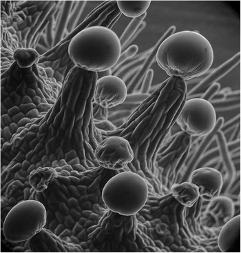
Figure 1 Cannabis sativa flower showing resin nodules with glandular multicellular capitate triochomes imaged at 5 kV and 15 mm working distance. This was one of the first SEM images to appear in a commercial motion picture (stood in for “snake scale” in Ridley Scott’s 1982 Blade Runner). Image taken in 1973 [Reference Scharf2, Reference Scharf7]. Image width = 156 µm.
Materials and Methods
Specimen preparation
To simplify mounting of live specimens on an SEM stub, insect and arachnid specimens were first anesthetized with refrigeration of approximately 38°F or with CO2 and, if necessary, were very gently blown off with compressed air. Interestingly, most live insects and arachnids tend to preen themselves and remove dust from their bodies. Thus, these live specimens were usually mounted by adhering the rear legs or the very rear of the body to the stub using denatured alcohol and graphite (DAG), which allowed preening to continue. For botanical specimens, care was taken to keep cut surfaces to a minimum, such as cutting and mounting by the stem only whenever possible. This slows dehydration and keeps outgassing to a minimum. In many cases insects were found on botanical specimens and left there without any interference while the plant specimen was attached to the specimen stub.
Instrumentation
An ETEC Autoscan SEM with a tungsten thermionic electron gun, employing an oil diffusion high-vacuum pump, was used for early research and subsequent follow-up work. Most SEMs in the 1970s yielded 4” × 5” images with about 1,000 lines, so the line spacing was just below what the eye can detect. The ETEC instrument allowed the user to vary the number of lines per frame up to 4,000 lines, even though the cathode ray recording tube had a resolution of 2,500 lines, allowing acquisition of images that could be enlarged significantly from the negative with photographic prints having been successfully made and exhibited up to 5 ft × 5 ft. Thus, until about 1992, images were recorded on 4 × 5 film, including Polaroid PN-52, PN-55, Kodak Plus-X, and Ilford FP-4. In 1992 a 4Pi digital acquisition card was used in an Apple Macintosh computer for early experimentation. Beginning in 1993 a Gatan Digiscan with Digital Micrograph software was used for multi-channel digital image acquisition on an Apple Macintosh computer.
Key to this technique is a vacuum system with a quick pumpdown time. The ETEC Autoscan’s valved vacuum diffusion pump system, with buffer tank and small specimen chamber, was ideal. This system could be pumped down to 5 × 10⁻⁵ torr (the system HV turn-on vacuum) in 60–70 seconds. The fast pump-down was essential for many of the more delicate specimens because they could dehydrate in a few minutes, and fast pumping gives the operator more work time. Many specimens could be observed and imaged for tens of minutes at magnifications from 10× to approximately 5,000×.
Imaging
Because insects sit higher than the specimen stub by several millimeters, imaging with a large depth of field is usually desirable. Because of the electron optical column design and the position of the objective aperture in the final lens, the most-used aperture size for imaging in the ETEC was 150 µm. This aperture was a good compromise between beam intensity and depth of field for most users. Larger apertures were used occasionally for imaging but more often for x-ray analysis. However, by employing a smaller aperture of 100 µm or so, a relatively long working distance (up to 40 mm between the specimen and the bottom of the final lens), and careful use of electronic dynamic focus, an entire specimen can be brought into focus while displaying fine surface detail. It should be noted that very long working distances tend to visually flatten images and slightly degrade resolution, therefore moderate working distances of 10 mm to 20 mm were more routinely used, preserving the perception of depth in the images. This advantage of the SEM is particularly useful in imaging insects and larger botanical specimens. A high specimen tilt, 90° or so, was used in many situations in order to have a good portrait perspective and have a darkened, non-distracting background.
Through trial and error, a beam accelerating voltage of approximately 5 kV was found to give the best results, producing just the right amount of surface detail and beam penetration on live specimens for acceptable photographic image quality. Accelerating voltages of 2–3 kV were useful in some situations. A moderate condenser lens setting (for spot size/beam current) was used as a starting point. Optimum condenser settings were found for particular specimens and magnification ranges by trial and error. Fast scan rates (short beam dwell per picture point) allowed the use of larger beam currents for good quality images (high signal to noise [S/N]) or just observation. Slower scans (longer beam dwell) required lower beam current to avoid beam damage and specimen charging.
Examining live insects, and hydrated specimens in general, requires keeping observation time to a minimum. Standard practice was to perform critical focusing on images at a magnification at least ten times higher than that to be used for recording. This focusing would be accomplished at a place on the specimen that would be out of the recorded frame whenever possible. Images were generally recorded from the high-resolution recording CRT, which was calibrated and standardized at a lens aperture of f 8 and 2,500 lines per frame with a total record time of 60–70 seconds. Black levels and highlight saturation were experimentally determined for each type of film used or calibrated to the dynamic range of the digital acquisition hardware.
Results
Figures 1 through 6 show that early trials and experimentation in 1973 and 1974 yielded results of surprisingly good quality. All these images were made of insects or flora in their natural state as live unfixed specimens. Many of these and later images were subsequently widely published in trade and consumer publications and shown in exhibitions [Reference Scharf2–Reference Scharf7]. Figure 7 [Reference Scharf8] shows a more recent, digitally acquired, color image made with the Wideband Multi-Detector Color Synthesizer system [Reference Scharf9].
Discussion
It was not uncommon for many live insects and arachnids to keep moving for quite some time while being observed, ruining many a still image. So beginning in 1988, some of the first SEM, NTSC-TV video recordings were made direct to S-VHS and later to DVCAM format. This was possible because the ETEC Autoscan allowed real-time NTSC or PAL video scanning with a separate video scan generator and alternate high speed deflection coils used exclusively for the TV scanning system. The TV scan rates resulted in lower beam dwell times at each image point and thus made possible the use of larger spot sizes with more current, improving S/N. Similar to the still images, as the magnification increases, the spot size must decrease causing a smaller beam current and a lower S/N. The remedy here was to use a larger final aperture (150 to 200 µm) when needed and a video frame averager, which allowed video imaging with reduced noise even at high magnifications. But high magnifications were not needed for most live, uncoated samples; indeed, most images were obtained at magnifications of only a few hundred times. This was partly because low magnifications captured large fractions of the organism and partly to maintain a large depth of field.
Using the older film recording technique, the final outcome of an image was not usually known until the film was developed and a contact sheet made, taking several hours. Modern digital image acquisition makes SEM imaging more assured because it is possible to extensively vary scanning parameters and see the resulting image immediately, even during the scan. If there is a problem, we can correct it and quickly acquire another image. It is also useful to do a low-resolution, fast scan to check the situation, and if things look good, proceed with a slower, high-resolution final scan.
It is interesting to note that over many years of observations no serious SEM damage was ever observed from the outgassing of hydrated specimens. In fact, in a few cases insects and spiders were still alive after examination and were returned to the garden.
Conclusion
Images of live, uncoated biological samples provide additional scientific data due to the variance of surface chemical and elemental composition, making for a more interesting and informative photographic quality than images of fixed, dried specimens with a uniform metal coating.
The technique described here still has usefulness today, especially for those who may not have access to an ESEM, VP-SEM, or a Cryo-SEM. And unlike using a VP-SEM or ESEM, where short working distances are required, images may be recorded at any working distance for excellent depth of field.

Figure 2 Gladiola flower (Gladiolus, family Iriaceae) petal surface showing individual cells at 5 kV and 14 mm working distance. Image taken in 1974 [Reference Scharf7]. Image width = 437 µm.

Figure 3 Black ant (Tapinoma sessile) at 5 kV and 24 mm working distance. These ants eat honeydew, which is made by aphids and scale insects, and other sugary foods. These ants are commonly found in the home. A 5 ft × 5 ft photographic print was made of this image for a museum exhibition. Image taken in 1974. Image width = 581 µm.

Figure 4 Compound eye of a house fly (Fannia canniculartis) at 5 kV and 20 mm working distance. Each facet is an individual eye with its own lens and retina. Image taken in 1974 [Reference Scharf7]. Image width = 508 µm.

Figure 5 Immature strawberry flower (Fragaria, family Rosaceae) at 5 kV and 19 mm working distance. Immature fruit showing achenes with stigmas and styles protruding. Image taken in 1976 [Reference Scharf7]. Image width = 2.54 mm.

Figure 6 Moth fly (family Psychodidae) at 5 kV and 19 mm working distance. These harmless 1 mm flies can enter the house through a window screen and breed in sink and bathtub drains. Image taken in 1976 [Reference Scharf7]. Image width = 271 μm.

Figure 7 Anopheles stephensi mosquito (female) at 5 kV and 14 mm working distance. This species is predominant in Asia and is a disease vector for the Plasmodium protozoa that causes malaria. Color synthesized with the Scharf multi-detector color SEM. Image taken in 2006. Image width = 2.26 mm.
Copyright Statement
All images in this article are copyright © by David Scharf and may not be used without permission. To see more images by David Scharf visit www.scharfphoto.com.


