


1. Introduction
Capillary driven flows arise in many situations when a wetting fluid displaces a non-wetting fluid. Important examples include the classical capillary imbibition flow in which a fluid is drawn along a capillary tube, as described by Washburn, Lucas, Bell and Cameron (WLBC), and the capillary driven flows along a corner formed by the intersection of two planes (Lucas Reference Lucas1918; Bell & Cameron Reference Bell and Cameron1905; Washburn Reference Washburn1921; Weislogel & Lichter Reference Weislogel and Lichter1996). In the general case, the flow is three-dimensional, but in the case of a narrow angle V-shaped channel, the flow may become approximately two-dimensional. The capillary pressure jump between the two fluids depends on the location of the interface across the channel, being proportional to  $\sigma /b$, where $b$ is the local gap width and $\sigma$ the surface tension. The flow may then be driven along the channel by the gradient of capillary pressure associated with variations in the location of the interface across the channel, as sketched in figure 1. The capillary driven flow of a single fluid along such a narrow wedge has been described by Romero & Yost (Reference Romero and Yost1996) and Weislogel & Lichter (Reference Weislogel and Lichter1996). They showed that, at early times, the fluid is drawn out by the gradient of capillary pressure into the narrower side of the channel, while the fluid supplying this advancing tongue is supplied by a receding front on the wider side of the channel, with the motion being described by similarity solutions in which the interface moves at a speed proportional to $t^{-1/2}$. They also considered the motion of a finite volume of fluid which spreads out along the thin part of the channel from an initially localised region, and demonstrated that this is governed by a different class of similarity solution, in which the front spreads with speed decaying as $t^{-3/5}$.

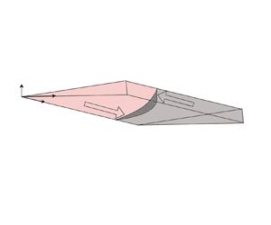
Figure 1. (a) Cartoon displaying early time behaviour where there is a fully saturated region of wetting fluid in the range  $-x_s< x< x_s$. (b) At later times the two receding fronts meet and the wetting fluid slumps at the origin as the current extends along the channel. (c) As the flow is symmetrical about $x=0$, for simplicity we only consider the region $x>0$. The channel thickness varies linearly with cross-channel position with the leading wetting front migrating through the thinnest region of the channel. (d) Interface curvature at two interface positions. The curvature at the interface increases toward the thin boundary, leading to a capillary pressure gradient which drives flow.
In the present contribution, we develop this analysis to consider the capillary driven flow of a wetting fluid into a channel which is initially saturated with a second immiscible fluid of different viscosity. We consider the capillary driven spreading of a finite volume of the wetting fluid, assuming that it fills the width of the channel along a finite region and illustrate the control of the mobility ratio between the two fluids on the imbibition flow, contrasting new solutions for the early and later time flow with earlier studies which focussed on a single fluid. We also consider the case in which a channel, initially filled with one fluid, is adjacent to a reservoir containing an immiscible and preferentially wetting fluid which is maintained at a different pressure from the far-field pressure in the channel. We show that, with a sufficiently small pressure difference, a counterflow with zero net flux develops in the channel driven by the capillary pressure, in which the wetting fluid only partially saturates the channel. In contrast, with a larger pressure difference, we show that the wetting fluid fills the channel, leading to a net flow in the along-channel direction, which represents a generalisation of the WLBC-type capillary imbibition flow.
Such capillary imbibition flows may be important in situations in which fluid is injected into a fractured rock, for example with CO2 geo-sequestration, whereby supercritical CO2 is injected into a saline aquifer. In this case, the CO2 will initially flood the high permeability primary fractures within the formation leading to a dispersed zone of CO2 within the formation. Typically, such fractures intersect secondary fractures, which are initially filled with brine. Over time, the capillary imbibition flows described herein may lead to further dispersion of the CO2 into the formation driven by the exchange of CO2 and water between the primary and secondary fractures. This process may be critical in assessing the storage capacity of the reservoir, and the lateral extent of the CO2 plume within the reservoir.
Our model also provides a physical analogue to capillary imbibition flows through a porous rock (Handy Reference Handy1960; Bear Reference Bear1975; Alyafei & Blunt Reference Alyafei and Blunt2018). In porous media, the flow is described in terms of the saturation  $s$ of the wetting fluid within the pore space, and empirical laws for the capillary pressure $P_c(s_i)$ and relative permeability of each phase, $k_i(s)$ are expressed in terms of this saturation. The model developed herein for flow in a triangular shaped channel provides an analogue and exact analytical model for such porous medium flows, where the width of the flow across the channel is equivalent to the saturation in the porous layer. This analogy is complementary to the model of Lajeunesse et al. (Reference Lajeunesse, Martin, Rakotomalala, Salin and Yortsos1999), in which it was demonstrated that the displacement of one fluid by second in a cylinder or a constant gap width Hele-Shaw cell is analogous to the Buckley–Leverett fractional flow model for displacement flow in a porous medium. The inclusion of a variable thickness across the channel, leads to variations in the capillary pressure analogous to the saturation dependence of the capillary pressure in a porous layer.
We have arranged the paper as follows. First, we derive the equations for the counterflow in a finite width channel, and describe new solutions for the spreading of a finite volume of wetting fluid at short and long times as it displaces the non-wetting phase. We then discuss how a buoyancy contrast between the two fluids impacts the flow when gravity acts both across and along the channel, illustrating the control of the flow in terms of the Bond number. We then present a new class of solutions corresponding to an exchange flow between a channel and reservoir of fixed pressure, establishing a regime diagram to delineate the condition in which a counterflow and a co-flow develop. Finally, we explore the analogy between the present model and the models typically used for capillary driven imbibition in a porous layer.
2. Immiscible exchange between two fluids
We consider the displacement of one fluid by a second, preferentially wetting fluid, along a channel of width  $0< y< H$ and thickness $b(y)$ – see figure 1. As the interface between the fluids spreads out along the channel, the curvature becomes dominant in the cross-channel direction and,to leading order, we can write the capillary pressure at the interface as $\sigma /b$, where $\sigma$ is the surface tension. If the gradient of the channel thickness is sufficiently shallow so that $\max (b)\ll H$ then, to leading order, the resulting capillary pressure gradient acts in the along-channel direction and the boundary layer connecting the fluid to upper and lower faces of the channel is much smaller than the extent of the fluid–fluid interface. Then, in the limit where the interface extends a distance along the channel which is much greater than $H$, the flow becomes approximately unidirectional, with the pressure gradient in each fluid phase being constant at each point along the channel. The flow speed at a point $(x,y)$ is then given by
 $$\begin{gather} u_w ={-} \frac{b(y)^{2}}{12 \mu_w}\frac{\partial P_w }{\partial x}, \end{gather}$$
 $$\begin{gather}u_{nw} ={-} \frac{b(y)^{2} }{12 \mu_{nw}}\frac{\partial P_{nw} }{\partial x}, \end{gather}$$
where  $\mu$ is the fluid viscosity and the subscripts $w$ and $nw$ denote the wetting and non-wetting phases respectively. The flux of the wetting fluid and non-wetting fluid at point $x$ along the channel is then given by
 $$\begin{gather} Q_w ={-}\frac{1}{12\mu_w} j(0,w) \frac{\partial P_w }{\partial x}, \end{gather}$$
 $$\begin{gather}Q_{nw} ={-}\frac{1}{12\mu_{nw}} j(w,H) \frac{\partial P_{nw} }{\partial x}, \end{gather}$$
where
 \begin{equation} j(w_1,w_2) = \int_{w_1}^{w_2} b(y)^{3} \,{\textrm{d} y}, \end{equation}
where  $w_1$ and $w_2$ are arbitrary coordinates along the $y$ axis. The capillary pressure gives rise to a pressure jump across the fluid interface. Given that the capillary pressure is
 \begin{equation} P_c ={-}\frac{\sigma}{b(w)}, \end{equation}
we can relate the pressure in the wetting fluid to that of the non-wetting fluid with the relationship
 \begin{equation} P_{nw}(x,t) = P_{w}(x,t) - P_c(x,t) = P_{w}(x,t) + \frac{\sigma}{b(w)}. \end{equation}
 If there is a net flux  $Q$ along the channel, then after some algebra, we find that the local conservation of mass has the form
 \begin{equation} b(w)\frac{\partial w}{\partial t} + Q \frac{\partial }{\partial x}J(w) = \frac{\sigma M}{12\mu_{w}}\frac{\partial}{\partial x}\left(\frac{J(w)j(w,H)}{b(w)^{2}}\frac{d b}{dw}\frac{\partial w}{\partial x}\right) \end{equation}
where the viscosity ratio  $M = \mu _{w}/\mu _{nw}$ and the fractional flow of the wetting phase $J(w)$ is given by
 \begin{equation} J(w) = \frac{j(0,w)}{j(0,w) + Mj(w,H)}. \end{equation}
 The solutions of (2.6) depend on the boundary conditions and the details of the channel thickness with position across the channel. In the following, we assume that  $b(w)=\lambda w$ for $0< w< H$, where $\lambda$ is the gradient of aperture width across the channel.
We consider two problems. First, the spreading of a finite volume of wetting fluid initially located in the region  $-L< x< L$, which fills the width of the channel, while the remainder of the channel is filled with non-wetting fluid. Second, the spreading of a wetting fluid from a reservoir of pressure $P$, at $x=0$, which opens into the channel, and we consider the flow in $x>0$.
3. Finite release
For a finite release we consider the volume of wetting fluid in the region  $0< x< L$ which ultimately spreads into the region $x>0$. The leading front of the wetting fluid, $x_f$, propagates away from $L$ and the trailing front of the current, $x_s$, which runs along the thick boundary, propagates toward the origin. It is convenient to introduce dimensionless variables $w = \hat {w}H, x = \hat {x}L$ and $t = \hat {t}\tau$ where,
 \begin{equation} \tau = \frac{48L^{2}\mu_w}{\lambda H\sigma} \end{equation}
leading to the dimensionless governing equation
 \begin{equation} \hat{w}\frac{\partial \hat{w}}{\partial \hat{t}} = M\frac{\partial}{\partial \hat{x}}\left(\frac{\hat{w}^{2}(1-\hat{w}^{4})}{\hat{w}^{4} + M(1-\hat{w}^{4})}\frac{\partial \hat{w}}{\partial \hat{x}}\right), \end{equation}
for the shape of the interface  $\hat {w}$. In figure 2(a) we present a series of numerical calculations which illustrate the variation of the leading edge of the wetting fluid as a function of time. In the figure, we see that the front grows at a rate proportional to $t^{1/2}$ at early time and at a rate proportional to $t^{2/5}$ at late time. The transition depends on the value of $M$, and is somewhat slower than the rate of advance of the wetting fluid in the asymptotic case $M \rightarrow \infty$ corresponding to the case in which the non-wetting fluid viscosity tends to zero.

Figure 2. (a) Variation of the leading edge of the current as a function of time, for  $M = 0.1$, 1, 10 and for a single wetting fluid ( $M=\infty$). As $M$ increases the transition from early time self-similarity to late time self-similarity shortens. For $M =10$ the front position is almost indistinguishable from that of a single fluid propagating in an empty channel. The dashed blue and green lines are a guide for the eye and show the theoretical gradients of the early and late time power laws. (b) Early time confined exchange flows of $M = 0.01$, 0.1, 1, 10 and 100. Note that $M=100$ is very similar to the solution for a single wetting fluid (red dashed line). We also show the similarity solution for $M=1$ (blue dotted line) which shows a strong agreement with the numerical simulation. (c) The position of $\eta _f$ (solid line) and $\eta _s$ (dashed line) as a function of mobility ratio. (d) The variation of the $\hat {w}$ as a function of along-channel position at time $\hat {t} = 0$, 1, 10, 100 and 1000 for the case $M = 1$.
At early times when the current is confined by the channel walls, we can therefore expect a solution of the form  $\hat {w}$ = $f(\eta )$ where $\eta = \hat {x} / \hat {t}^{1/2}$ and for which $f$ satisfies the equation
 \begin{equation} {-}\frac{\eta}{2}ff' = M\left(\frac{f^{2}(1-f^{4})f'}{f^{4} + M(1-f^{4})}\right)' \end{equation}
subject to the boundary conditions that at  $\eta = \eta _f, f= 0$ and $f' = - \eta _fM / 4$, while at $\eta = \eta _s, f = 1$ and $f' = 0$ - where $\eta _f$ and $\eta _s$ are the leading and trailing fronts of the wetting fluid in similarity coordinates respectively. The solution of (3.3) is shown in figure 2(b) for the cases $M= 0.01$, 0.1, 1, 10 and 100. Full numerical solutions are compared with the similarity solution for the case $M = 1$. It is seen that as $M$ becomes larger and the relative mobility of the non-wetting fluid increases then the wetting fluid advances through a greater cross-channel region, so that it can access wider parts of the channel. In contrast, when the wetting fluid is of relatively low viscosity, it spreads along a thin region near the narrowest part of the channel. When $M\gg 1$, (3.2) reduces to the simplified form
 \begin{equation} {-}\frac{\eta}{2}ff' = \left(f^{2}f'\right)', \end{equation}
which is consistent with the model of Romero & Yost (Reference Romero and Yost1996) for a single capillary current running along a V-shaped groove, with solution given by the red-dashed line in figure 2(b). We can also find the limit corresponding to a single non-wetting fluid by taking  $M\ll 1$. We can re-scale (2.6) with respect to the non-wetting fluid by defining a new dimensionless time $t^{*}$, so that $t = t^{*}\tau ^{*}$ where
 \begin{equation} \tau^{*} = \frac{48L^{2}\mu_{nw}}{\lambda H\sigma}. \end{equation}
We therefore take a new similarity variable  $\eta ^{*} = \hat {x}/\sqrt {t^{*}}$ and the governing equation in similarity coordinates becomes
 \begin{equation} -\frac{\eta^{*}}{2}ff' = \left(\frac{f^{2}(1-f^{4})f'}{f^{4} + M(1-f^{4})}\right)', \end{equation}
which in the limit  $M\ll 1$ becomes
 \begin{equation} -\frac{\eta^{*}}{2}ff' = \left(\frac{(1-f^{4})f'}{f^{2}}\right)', \end{equation}
which indeed is the equation for a single non-wetting fluid along a V-shaped groove. Detailed solutions for a non-wetting fluid can be found in Appendix A.
Continuing with our initial example, at later times the two fronts of non-wetting fluid advancing into the wetting fluid will meet. Subsequently the wetting fluid spreads out along the narrow part of the channel, occupying a progressively thinner fraction of the channel. We see from figure 2(a) that in this regime, asymptotically the current propagates at a rate proportional to  $\hat {t}^{2/5}$. Indeed, the system admits solutions of the form $\hat {w} = \hat {t}^{\alpha } f({\hat {x}}/{\hat {t}^{\beta }})$, where $\alpha = -1/5$ and $\beta = 2/5$. This flow is directly analogous to the capillary driven spreading of single wetting fluid along a sharp corner. Figure 2(c) shows the position of the advancing front $\eta _f$ (solid line) and the retreating front $\eta _s$ (dashed line) as function of mobility ratio. We can see that the lateral extent of the early time similarity solution increases with mobility toward the maximum at $M = \infty$. The late time spreading of the current is illustrated by figure 2(d) where we show current profiles for $\hat {t} = 1$, 10, 100 and 1000. Note that the backward propagating front $\hat {x}_s$ reaches the origin at around $\hat {t} = 1$, where then the transition to late time self-similar behaviour begins.
3.1. Impact of cross-channel component of gravity
In many applications, there may also be a component of gravity in the cross-channel direction, in which case there may be a buoyancy force associated with any density difference  $\Delta \rho$ between the two fluids. Where $\Delta \rho = \rho _w - \rho _{nw}$, with $\rho _w$ and $\rho _{nw}$ being the density of the wetting and non-wetting fluid, respectively. We consider the case where gravity acts in the negative $y$ direction, the wetting fluid is denser than the non-wetting fluid. The local conservation law for the evolution of the interface can then be generalised to include the buoyancy force acting in tandem with the capillary force, leading to the equation
 \begin{equation} b(w)\frac{\partial w}{\partial t} = \frac{M}{12\mu_{w}}\frac{\partial}{\partial x}\left(\left[\frac{\sigma}{b(w)^{2}}\frac{\textrm{d}b}{\textrm{d}w} + \Delta\rho g\right]J(w)j(w,H)\frac{\partial w}{\partial x}\right). \end{equation}
If we again let the channel profile take the form  $b(w) = \lambda w$ and let $w = \hat {w}H, x = \hat {x}L$ and $t = \hat {t}\tau$ we arrive at the dimensionless governing equation
 \begin{equation} \hat{w}\frac{\partial \hat{w}}{\partial \hat{t}} = M\frac{\partial}{\partial \hat{x}}\left(\frac{\hat{w}^{2}(1-\hat{w}^{4})(1+Bo\hat{w}^{2})}{\hat{w}^{4} + M(1-\hat{w}^{4})}\frac{\partial \hat{w}}{\partial \hat{x}}\right), \end{equation}
where  $Bo = {\lambda \Delta \rho g H^{2}}/{\sigma }$. In figure 3(a) we present numerical solutions illustrating the position of the leading edge of the flow when a finite volume of wetting fluid is released from the region $-L< x< L$, and an exchange flow with the original non-wetting fluid develops. At early times, the leading front migrates at a rate proportional to $t^{1/2}$ with the flow speed increasing with Bond number, as gravity becomes progressively more dominant. Once the receding front reaches the point $x=0$, the wetting fluid separates from the top boundary and the flow adjusts to a long thin slumping flow. It is seen that with a large Bond number $(Bo =100)$, when gravity effects dominate, the front of the current steepens relative to those flows with smaller $Bo$, because in the wider parts of the channel the flow upstream is faster than the pure capillary driven flow.

Figure 3. (a) The  $\ln - \ln$ plot of front position vs time for $Bo = 0$, 10 and $100$. We can see for higher Bond numbers an intermediate regime which is dominated by gravity effects. This length of this intermediate regime increases with increasing Bond number. The dashed lines are a guide for the eye showing the theoretical power laws of the confined, gravity driven and capillary driven regimes respectively. (b) Confined gravity–capillary exchange solutions shown for $Bo = 0$, 10 and $100$. (c) Late time shapes for $Bo = 100$ at $\hat {t} = 1$, 10, 100 and 1000. (d) Scaled similarity shape of a gravity current (red dashed line) and a capillary current (blue dashed line). We can see how the scaled numerical profiles adjust from the gravity limit toward the capillary limit for the $Bo =100$ case across the times $\hat {t} = 0.2$, 10 000 and 20 000.
For large Bond numbers there is an intermediate gravity dominated regime. Indeed, in the absence of capillary forces, a finite volume of fluid spreading through a V-shaped channel will propagate at a rate proportional to  $t^{2/7}$ (Takagi & Huppert Reference Takagi and Huppert2007) as seen in figure 3(a). However, at late times once $Bo\hat {w}^{2} \ll 1$ the capillary dominated solutions of (3.2) apply with the current ultimately spreading as $t^{2/5}$. Figure 3(b) shows the self-similar behaviour of the early time solutions, where $\hat {x}_s> 0$ for $Bo = 0$, 10 and 100. It can be seen that with increasing Bond number, the wetting fluid migrates more rapidly. In figure 3(c) we illustrate the evolution of the current shapes at late time. For $Bo =100$ the shape adjusts from that of a gravity current with a large gradient at the leading edge to that of a capillary current at later times, with a shallower gradient at the nose. In figure 3(d) we see three scaled current shapes at $\hat {t} = 0.2$, 10 000 and 20 000 for $Bo = 100$. The red dashed line indicates the shape of a gravity driven fluid in a V-shaped channel (Takagi & Huppert Reference Takagi and Huppert2007) and the blue dashed line shows the shape of a single capillary current from (3.4). The plot shows how the current adjusts from the gravity driven shape at early times toward the capillary current shape asymptotically.
3.2. Impact of along-channel component of gravity
Now consider a channel which is tilted at some angle  $\theta$ to the horizontal, so that there is an along-channel as well as a cross-channel component of gravity – see figure 4. Again, we consider a wetting fluid which initially fills the region $-L< x< L$.

Figure 4. Cartoon illustrating the shock-like dynamics of an immiscible preferentially wetting current acting under gravity forces both in the across- and along-channel directions. The along-channel component of gravity leads to an increase in the interface speed with increasing  $y$ – as the thickness increases. This leads to a steepening of the current near the nose and a region where the current width rapidly drops to zero.
If the channel is inclined so that  $-L$ is up-slope from $L$, then the wetting fluid will migrate at a Darcy speed according to
 \begin{equation} u_w ={-} \frac{b(y)^{2}}{12\mu_w} \left(\frac{\partial P_w}{\partial x} - \rho_w g \sin\theta\right). \end{equation}
Given that we are considering a sealed channel containing a constant volume of fluid, we can follow the approach of § 2 by equating the flux of the two fluids in order to eliminate the pressure gradient. Upon doing this we arrive at the advection–diffusion-type equation
 \begin{gather} b(w)\frac{\partial w}{\partial t} + MG \frac{\partial}{\partial x}J(w)j(w,H) = \frac{M\sigma}{12\mu_{w}\lambda}\frac{\partial}{\partial x}\left[\left(1 + \frac{\lambda\Delta\rho g w^{2}}{\sigma}\right)\frac{\partial w}{\partial x}\frac{J(w)j(w,H)}{w^{2}}\right], \end{gather}
where
 \begin{equation} G = \frac{\Delta \rho g \sin \theta}{12\mu_{w}}. \end{equation}
By applying the same channel profile and scalings as before we arrive at the dimensionless equation
 \begin{gather} \hat{w}\frac{\partial \hat{w}}{\partial \hat{t}} + MBo\sin\theta \frac{\partial}{\partial x}\left(\frac{\hat{w}^{4}(1-\hat{w}^{4})}{\hat{w}^{4} + M(1-\hat{w}^{4})}\right) = M\frac{\partial}{\partial \hat{x}}\left(\frac{\hat{w}^{2}(1-\hat{w}^{4})(1+Bo\hat{w}^{2})}{\hat{w}^{4} + M(1-\hat{w}^{4})}\frac{\partial \hat{w}}{\partial \hat{x}}\right). \end{gather}
As the leading edge of the current migrates down the channel, we expect that the width of the current becomes small so that in the limit  $\hat {w}\ll \min \{1,Bo^{-1/2},M^{1/4}\}$, (3.13) becomes
 \begin{equation} \hat{w}\frac{\partial \hat{w}}{\partial \hat{t}} + 4Bo\sin\theta\hat{w}^{3}\frac{\partial \hat{w}}{\partial \hat{x}} = \frac{\partial}{\partial \hat{x}}\left(\hat{w}^{2}\frac{\partial \hat{w}}{\partial\hat{x}}\right). \end{equation}
If we let  $\varGamma = 4Bo\sin \theta$, then we also expect that for large $\varGamma$ the advective term will dominate the along-channel migration (Huppert & Woods Reference Huppert and Woods1995). The speed of the interface at a constant width will be, to leading order
 \begin{equation} \frac{\textrm{d}\hat{x}}{\textrm{d}\hat{t}} = \varGamma\hat{w}^{2} \end{equation}
leading to the solution
 \begin{equation} \hat{x}(\hat{t}) = \hat{x}(0) + \varGamma\hat{w}^{2}\hat{t}. \end{equation}
Since the flow speed increases with the thickness of the current, the leading edge of the current continually steepens, and eventually leads to the formation of a region in which the depth rapidly drops to zero. To leading order we can describe the front of the flow in terms of a discontinuous shock-type solution (Whitman Reference Whitman1974), as has been described in the analogous problem of a gravity current moving down a slope in a uniform porous medium (Huppert & Woods Reference Huppert and Woods1995). We first present solutions for this leading-order model of the front of the current and then describe in detail the structure of the transition to zero depth across this shock, by accounting for the effect of the gradient of capillary pressure on the flow. The position of the shock front is given by the dimensionless relation for volume conservation
 \begin{equation} \int_{0}^{\hat{x}_{shock}}\hat{w}^{2}\,\textrm{d}\kern0.7pt\hat{x} = 1, \end{equation}
leading to the result
 \begin{equation} \hat{x}_{shock} = \hat{x}(0) \pm (\hat{x}(0)^{2} + 4\varGamma \hat{t})^{1/2}. \end{equation}
We can also find the envelope through which the current sweeps by combining (3.16) and (3.17) and thereby express the width of the current at the shock,  $\hat {w}_{shock}(\hat {x}_{shock})$. We neglect $\hat {x}(0)$ which is small relative to the current extent at late times in order to arrive at the approximate relation
 \begin{equation} \hat{w}_{shock} = \left(\frac{4}{\varGamma\hat{t}}\right)^{1/4}. \end{equation}
 Figure 5(a) shows numerical solutions to (3.13) for  $Bo =100$ and $M=1$ at $\hat {t} = 1$, $10$ and 100, compared with the approximate shock solutions. We can see that there is a reasonable agreement with some offset where the analytical solution (red line) is ahead of the numerical solution from the full equation. This is because we have neglected the diffusive terms of (3.13) in our shock analysis, leading to a slight over prediction of the shock position downslope. At later times this offset becomes very small as a fraction of the total current length and the current height matches the analytical prediction (blue dashed line) very closely.

Figure 5. (a) Numerical solutions of (3.13) for a pulse of fluid initially filling the channel in the range  $-1<\hat {x}<1$ with $\theta = 10$, $Bo = 100$ and $M=1$ at times $\hat {t} = 1$, 10 and 100, plotted with the analytical shock solutions (red lines) given by (3.18) and (3.19). We also display the fluid envelope showing $W_{shock}$ as a function of $\hat {x}_{shock}$ (blue dashed line). (b) Boundary layer at the leading front of the wetting fluid moving downslope. The scaled nose shape from the numerical solution to (3.13) at $\hat {t} = 1$ (dash-dotted line), 10 (dashed line), 100 (solid line) and 1000 (dotted line) for $Bo = 100$, $\theta = 10$, the red line is the analytical shape given by (3.24).
3.2.1. Capillary boundary layer
From (3.19) we expect the width of the current to wane at a rate  $\hat {t}^{1/4}$ across the shock. To model the detailed flow structure in this region we therefore substitute $\hat {w} = {\psi (\hat {x},\hat {t})}/{{\hat {t}}^{1/4}}$ into (3.14), resulting in
 \begin{equation} \frac{\psi}{\hat{t}^{1/2}}\frac{\partial \psi}{\partial \hat{t}} +4\varGamma\frac{ \psi^{3}}{\hat{t}}\frac{\partial \psi}{\partial \hat{x}} = \frac{1}{\hat{t}^{3/4}}\frac{\partial}{\partial \hat{x}}\left(\psi^{2} \frac{\partial \psi}{\partial \hat{x}}\right) \end{equation}
as  $\hat {t} \rightarrow \infty$ the first term becomes small so that
 \begin{equation} 4\varGamma\frac{ \psi^{3}}{\hat{t}^{1/4}}\frac{\partial \psi}{\partial \hat{x}} = \frac{\partial}{\partial \hat{x}}\left(\psi^{2} \frac{\partial \psi}{\partial \hat{x}}\right). \end{equation}
If we introduce the similarity variable  $\eta _b = ({\hat {x}_f - \hat {x}})/{\hat {t}^{1/4}}$ and integrate we find
 \begin{equation} \varGamma\psi^{4} ={-}\psi^{2} \frac{\partial \psi}{\partial \eta_b} + \kappa. \end{equation}
At  $\psi = \psi _{shock}$, $\psi ' = 0$, so that $\kappa = 4$. We therefore find that
 \begin{equation} \varGamma\psi^{4} ={-}\psi^{2} \frac{\partial \psi}{\partial \eta_b} + 4, \end{equation}
which we can integrate to find an implicit relationship between  $\eta _b$ and $\psi$
 \begin{equation} \eta_b = \frac{\tan^{{-}1}\left(\delta\psi\right) - \tanh^{{-}1}\left(\delta\psi\right)}{2^{3/2}\varGamma^{3/4}} , \end{equation}
where  $\delta = {\varGamma ^{1/4}}/{\sqrt {2}}$. Figure 5(b) shows that the structure of the front of the current as predicted by the full numerical solutions (black line) transitions with time toward the analytical profile found from (3.24).
4. Immiscible exchange from a reservoir through a channel
We now consider the different boundary condition in which the channel is connected to a reservoir of fluid at constant pressure, with the channel being oriented so that the  $y$-axis is vertical and the $x$-axis is horizontal (figure 6) . We consider the case in which the fluid in the reservoir is preferentially wetting and dense relative to the fluid originally in the channel. We explore the capillary driven exchange flow as the wetting fluid is drawn into the narrow part of the channel, driving out the original fluid back into the reservoir – see figure 6.

Figure 6. Cartoon showing the pressure driven injection of a dense, wetting fluid (red) into a channel filled with an immiscible fluid (grey). Here, the flux of the wetting fluid entering the channel is equal to the flux of the ambient fluid leaving the channel.
The flooding of the channel is controlled by two parameters; the reservoir pressure and the Bond number. There are two classes of solution for this problem. First, an exchange flow solution in which there is an exchange flow in the channel and second a solution with a net flow through the channel where the advancing front fills the entire channel width. Which of these two solutions develops depends on the pressure in the source reservoir and the Bond number in the channel as we describe below.
If we impose a source pressure  $P_S$ in the reservoir and a far field pressure in the channel $P_R$, then the pressure balance across the fluid interface at the reservoir–channel boundary is
 \begin{equation} P_S - P_R - \Delta \rho g h_0 ={-}\frac{\sigma}{\lambda h_0}, \end{equation}
where  $h_0$ is the height of the wetting fluid at the reservoir–channel boundary ( $x=0$). For convenience, we define a dimensionless pressure, equal to the pressure difference between the reservoir and the far field pressure over the characteristic hydrostatic pressure of the channel;
 \begin{equation} \hat{P} = \frac{P_S - P_R}{\Delta\rho gH}. \end{equation}
We then let  $h_0 = \hat {h}_0H$, where $\hat {h}_0$ is the dimensionless height of the wetting fluid at the reservoir–channel boundary, leading to the dimensionless relationship between $\hat {h}_0$ and $\hat {P}$
 \begin{equation} \hat{P}= \hat{h}_0 - \frac{1}{Bo\hat{h}_0}. \end{equation}
At the upper boundary,  $\hat {h}_0$ = 1. Equation (4.3) therefore suggests that the wetting fluid only partially floods the channel if
 \begin{equation} \hat{P} < 1 - \frac{1}{Bo}. \end{equation}
In this case, there is no net flow through the channel, and we expect a capillary driven counterflow to develop. Figure 7(a) displays a regime diagram based on (4.4) illustrating that for Bond numbers below a critical value ( $Bo =1$), the channel will flood at the origin for all positive $\hat {P}$ leading to a net flow through the aquifer, whereas for larger Bond numbers, an exchange flow will develop, with no net transport along the channel. Figure 7(b) shows the relationship between $\hat {P}$ and $\hat {h}_0$ for a range of Bond numbers in the case that an exchange flow develops. As can be seen from (4.3), $\hat {P} \approx \hat {h}_0$ for large Bond numbers. The partially filled channel solution has the form $w = f({\hat {x}}/{\hat {t}^{1/2}})$ where $f$ satisfies (3.3) in $\eta _f> \eta >0$ subject to the boundary condition $f(\eta _f)=0$ and $f(0) = \hat {h}_0$.

Figure 7. (a) Regime diagram showing how the channel flooding is controlled by the dimensionless pressure and the Bond number. Below a critical Bond number the channel floods at the origin for all positive pressures. When the Bond number is large ( $Bo>100$) the channel is partially filled where $\hat {P}<1$, for $\hat {P}>1$ the channel is always flooded at the origin as the difference between the reservoir pressure and the far-field pressure is greater than the characteristic hydrostat of the channel. (b) Variation of the height of wetting fluid at the origin as a function of dimensionless pressure in the reservoir, in the limit that the channel is partially flooded, for Bond numbers in the range 2–256.
In figure 8(a) we present numerical solutions showing the dependence of  $\eta _f$ as a function of the Bond number and the dimensionless source pressure. At lower pressures, the currents with lower Bond numbers have a greater lateral extent. This is because at lower pressures the width of the current decreases with Bond number and so the migration of current is predominantly limited by the narrow and therefore highly resistant region of the channel. At higher pressures, however, the depth of the wetting fluid at the origin is larger and so the buoyancy forces become more significant. At intermediate pressures there is a transition between these two regimes – as may be seen in by figure 8(b–d) by comparing the solutions with different Bond numbers.

Figure 8. (a) Variation of the position of the leading edge of the wetting fluid in similarity coordinates as a function of the pressure for Bond numbers 4, 16, 64 and 256 and for  $M = 0.1$ (dotted line), $M = 1$ (solid line) and $M = 10$ (dash-dotted line). The mobility of the fluid only influences the lateral extent appreciably for higher pressures. (b–d) Depth of the current as a function of position in the fracture for Bond numbers 4, 16, 64 and 256 at $\hat {P} = 0.1$, 0.4 and 0.7. Interestingly, at lower pressure the lower Bond number currents have a greater extent. As the reservoir pressure increases there is a reversal of this effect as more of the current moves through the higher permeability region of the channel at higher pressures, with the increased buoyancy force having a greater effect.
The other class of solution corresponds to the case in which the channel is fully flooded with the wetting fluid and there is a net flow along the channel. The detail of this solution depends on the far-field boundary condition and the viscosity of the two fluids. In the limit of a finite length channel in which the original non-wetting phase has relatively low viscosity, so that the main pressure drop is in the wetting fluid, then the solution may be approximated by taking  $M \rightarrow \infty$ and recovering the governing equation for a single wetting fluid; (3.4).
As shown by figure 7(a) we find solutions which flood the depth of the channel in the case
 \begin{equation} \hat{P}> 1 - \frac{1}{Bo}. \end{equation}
The pressure gradient in the fully saturated region  $0<\hat {x}<\hat {x}_s$ is given by
 \begin{equation} \frac{\textrm{d}\hat{P}}{\textrm{d}\hat{x}} = \frac{\hat{P} - 1 -\dfrac{1}{Bo}}{\hat{x}_s}. \end{equation}
At the point  $\hat {x}_s$ the flux in the saturated zone equals the flux supplied to the nose. We therefore match (4.6) with the expression from (3.9) for $M\gg 1$ in order to evaluate ${\partial \hat {w}}/{\partial \hat {x}}$ at $\hat {w} = 1$. This leads to the relation
 \begin{equation} \frac{\partial \hat{w}}{\partial \hat{x}} ={-} \frac{\hat{P} -1 + \dfrac{1}{Bo}}{\hat{x}_s\left(1+ \dfrac{1}{Bo}\right)}, \end{equation}
at  $\hat {w}=1$. In the limit of $M\gg 1$ we expect self-similar behaviour where the wetting current migrates at a rate proportional to $\hat {t}^{1/2}$. Substituting in the similarity variables $\hat {w} = f(\eta )$ and $\eta = \hat {x}/\hat {t}^{1/2}$, (4.7) becomes
 \begin{equation} f'(\eta_s) ={-}\frac{\hat{P} - 1 +\dfrac{1}{Bo}}{\eta_s\left(1 + \dfrac{1}{Bo}\right)}. \end{equation}
 Figure 9 shows calculations of the length and shape of the current across a range of  $\hat {P}$ and $Bo$. The figure illustrates that with larger Bond numbers the extent of the saturated region increases for a given value of $\hat {P}$. Also, as $\hat {P}$ increases, the current advances progressively more rapidly, as the flow becomes dominated by the reservoir pressure rather than the capillary pressure at the front. Note that from the rescaled shapes of the currents in the third column of plots, show that the scaled shape of the current nose remains approximately constant between pressures $\hat {P} = 0 - 4$.

Figure 9. The first, second and third rows of plots refer to the Bond numbers 0.5, 1 and 2 respectively. (a–c) Position of the leading (dashed line) and trailing (solid line) tip of the current nose in similarity space as a function of  $\hat {P}$. We can see that increasing Bond number will increase the relative length of the saturated zone to the length of the nose. (d–f) Shapes of the current across different $\hat {P}$ and $Bo$. (g–i) Scaled current shapes showing that the reservoir pressure has a weak influence on the shape of the current nose across the range.
We note that these solutions are analogous to the classical WLBC capillary imbibition solutions for a single wetting fluid. In the case that the viscosity of the original non-wetting fluid is significant, the details of these solutions are more complex, since the downstream flow of the non-wetting fluid also needs to be specified, and we leave the detail of this class of solution for subsequent investigation.
5. Analogue to flow in porous media
The capillary exchange flows described above in the confined channel provide an analogue physical system for the models of capillary exchange flows in porous media. This is of considerable interest in that the general models for flow in porous media are based on empirical laws for the relative permeability of each fluid phase and also the capillary pressure, as functions of the saturation of the wetting phase in the pore space (Handy Reference Handy1960; Bear Reference Bear1975; Alyafei & Blunt Reference Alyafei and Blunt2018). Lajeunesse et al. (Reference Lajeunesse, Martin, Rakotomalala, Salin and Yortsos1999) and Woods (Reference Woods2015) presented a series of analogue solutions for the Buckley–Leverett shock-type flows in a porous medium using the analogue system of a capillary tube or a Hele-Shaw cell in which the fraction of the area occupied by the invading fluid provided an analogue to the saturation. However, in those models the focus was on flow driven by an applied pressure and the effect of the partial filling of the tube or cell was to provide an analogue to the relative permeability. In the present model, we have also included an analogue for the variation of the capillary pressure with saturation.
It is known that the problem of capillary imbibition leads to counter flowing or co-flowing exchange flows, and there has been considerable interest in this class of problem in terms of inverting experimental observations of capillary imbibition to determine the capillary-saturation curves and the relative permeability of porous rocks (Alyafei & Blunt Reference Alyafei and Blunt2018).
Consider a wetting fluid imbibing into a porous region filled with non-wetting fluid under capillary forces. We assume that the wetting fluid initial occupies a region from  $0< x< x_0$ of maximum wetting saturation. The Darcy speeds of the two phases can be described as
 $$\begin{gather} u_w ={-}\frac{k_w k}{\mu_w}\frac{\partial P_w}{\partial x}, \end{gather}$$
 $$\begin{gather}u_{nw} ={-}\frac{k_{nw} k}{\mu_{nw}}\frac{\partial P_{nw}}{\partial x}, \end{gather}$$
where  $k_n$ and $k_{nw}$ are the relative permeabilities of the wetting and non-wetting phases, respectively. Using the pressure relationship between the two phases, $P_{nw} = P_w + P_c$, and the no-net-flow condition we can substitute the pressure gradient in the wetting phase and by mass conservation we find
 \begin{equation} \phi\frac{\partial s}{\partial t} ={-}\frac{\partial}{\partial x}\left(\frac{k_{nw} k F}{\mu_{nw}}\frac{\partial P_c}{\partial s}\frac{\partial s}{\partial x}\right) , \end{equation}
where  $s$ is the saturation of the wetting phase $\phi$ is the porosity of the porous matrix and
 \begin{equation} F = \left( 1 + \frac{k_{nw}\mu_w}{k_w \mu_{nw}}\right)^{{-}1} \end{equation}
represents the fractional flow of the wetting phase. We can define a normalised wetting saturation in terms of the maximum wetting phase saturation  $s_m$ and the minimum wetting phase saturation $s_r$ so that
 \begin{equation} \hat{s} = \frac{s - s_r}{s_m - s_r}. \end{equation}
 In order to proceed, we require a model for the relative permeability and the capillary pressure. In general in a porous rock, there is no simple relation for these properties, in contrast to the idealised V-shaped channel considered in this paper, for which the saturation  $\hat {s}$ is analogous to the width of the flow, $\hat {w}$. By comparing our model, (3.2), with (5.2), it follows that for the V-shaped channel the relative permeability has an effective value of $j(0,w)$ and $j(w,H)$ for the wetting and non-wetting phases, respectively. However, in a real porous rock, owing to the complexity of the geometry, empirical laws are typically introduced to describe the relative permeability and capillary pressure. As an illustration, in this paper, we adopt the classical empirical laws as described by Brooks & Corey (Reference Brooks and Corey1966), which may be used to describe the relative permeabilities of any homogeneous porous medium where the imbibing phase is strongly wetting;
 $$\begin{gather} k_w = \hat{s}^{4} \end{gather}$$
 $$\begin{gather}k_{nw} = (1-\hat{s}^{2})(1-\hat{s})^{2}. \end{gather}$$
In our analytical formulation for a V-shaped channel, the capillary pressure is simply given by  $\sigma /b^{2}$, however, for a porous medium we rely on the many parametrised empirical models of capillary pressure. Here, we draw on van Genuchten (Reference van Genuchten1980), who suggests that
 \begin{equation} P_c = \sigma \left(\frac{\phi}{k}\right)^{1/2}\left(\frac{1}{\hat{s}^{1/m} }-1\right)^{1/n}, \end{equation}
where  $m$ and $n$ are empirical constants which typically take a value between 2 and 3. Here, for simplicity we use $m = n = 2$. Using these empirical laws leads to the governing equation, which is analogous to the equation for $\hat {w}$ in the earlier parts of the work,
 \begin{equation} \frac{\partial \hat{s}}{\partial t} ={-}\frac{\sigma}{\mu_{nw}}\left(\frac{k}{\phi}\right)^{1/2}\frac{\partial}{\partial x}\left(k_{nw}F\frac{\partial P_c}{\partial \hat{s}}\frac{\partial \hat{s}}{\partial x}\right). \end{equation}
For comparison, we can examine the spreading of an interface between a wetting fluid in the region  $-L< x< L$ and a non-wetting fluid in the regions $x<-L$ and $x>L$. We can introduce dimensionless time and space coordinates $x = \hat {x}L$ and $t = \bar {t}\bar {\tau }$ and find the dimensionless expression
 \begin{equation} \frac{\partial \hat s}{\partial \bar{t}} = \frac{M}{mn}\frac{\partial}{\partial \hat{x}}\left(\frac{k_{nw}F\left(\hat{s}^{{-}1/m} - 1\right)^{1/n -1}}{\hat s^{(1/m +1)}}\frac{\partial \hat{s}}{\partial \hat{x}}\right), \end{equation}
where
 \begin{equation} \bar{\tau} = \frac{L^{2} \mu_w}{\sigma}\left(\frac{k}{\phi}\right)^{{-}1/2}. \end{equation}
 In figure 10 we present a numerical solution of (5.8). At early times, the solution is self-similar,  $\hat {s} = f(x/\sqrt {t})$, and the spreading of the fronts depends primarily on the viscosity ratio. Eventually the two spreading zones meet at $x=0$ and, subsequently, the wetting fluid spreads out, with saturation falling to progressively smaller values. At later times there is no fully saturated zone near the source and the saturation at the origin wanes as the volume of the wetting fluid stretches a long distance through the extent of the channel.

Figure 10. (a) Self-similar saturation profile in the limit where there is a region of the porous medium fully saturated near the source. Solutions displayed for  $M=0.1$, $1$ and 10. (b) Late time solutions where the medium is no longer saturated with wetting fluid near the source. The finite volume of fluid continues to migrate down the channel – so that the saturation of the fluid near the source wanes.
6. Conclusions
In this work we have examined the capillary driven exchange between two immiscible fluids in a channel of non-uniform width. The novel analysis of this work is to study the exchange of immiscible fluids in a non-uniform channel driven by both capillary and gravity forces. We also present new solutions for the exchange at a reservoir–channel boundary, where flow is driven by a pressure difference between the reservoir and the far-field channel pressure. We also propose that our model of a two fluid capillary driven exchange in a non-uniform channel may serve as an important analytical analogue to more complex empirical models of saturation in porous media.
We first develop similarity solutions for a confined fluid–fluid exchange, showing that the fluid fronts migrate at a rate proportional to  $t^{1/2}$. The confined exchange flow reduces to the well-known equations for single wetting and non-wetting fluids for high and low mobility ratios respectively. We then show that, if at later times the current becomes unconfined, the solutions will asymptote to those of a single fluid, with mobility ratio controlling this transition.
When gravity acts in tandem with capillary forces, there is a gravity dominated regime at intermediate times in which the current length scales as  $t^{2/7}$ which connects the early time confined behaviour $(x_f \propto t^{1/2})$ to the late time capillary driven behaviour $(x_f \propto t^{2/5})$. The persistence of this intermediate regime increasing with Bond number. We have also shown that an along-channel component of gravity leads to a shock-type structure at the leading front of the current. The position of the shock scales as $t^{1/2}$ and the width of the shock decreases at a rate proportional to $t^{1/4}$ with the flow structure in the shock dominated by capillarity.
Building on this analysis we look at pressure driven injection of a wetting fluid into a V-shaped channel from a reservoir filled with wetting fluid, again where gravity and capillarity both act to drive the flow. We show that it is possible for an exchange flow to develop at a range of reservoir pressures and Bond numbers. These exchange flows follow the  $t^{1/2}$ power law of a classical capillary current with the lateral extent governed by both pressure and Bond number. Interestingly, we show that, at low reservoir pressures, lower Bond number currents extend further into the channel than high Bond number currents, as the flow becomes restricted by the thinnest region of the channel. This limiting affect at low pressures also means that mobility ratio does not significantly affect the current extent at low pressures. At higher pressures, increasing mobility of the wetting phase results in a more rapid propagation of the current and as one would expect, the higher Bond number currents have a greater lateral extent.
As well as its relevance for flow in narrow fractures and channels, the model serves as an analogue to capillary imbibition in a porous medium. We show that the solutions to porous medium models which rely on empirical relationships between relative permeability and saturation are of a very similar form to our exact solutions in a Hele-Shaw cell.
Declaration of interests
The authors report no conflict of interest.
Appendix A. Non-wetting single fluid
For a single non-wetting fluid the interface curvature along the fluid boundary extends through the middle of the channel rather than along the channel walls – see figure 11(b). In the non-wetting fluid, there is a positive capillary pressure
 \begin{equation} P_c = \frac{\sigma}{b(w)}. \end{equation}
This drives the leading front of the fluid away from the thin wall of the domain and towards the wider region of the channel. Note that we neglect any friction which may impede the advance of the non-wetting fluid associated with the top surface of the channel.

Figure 11. (a) Cartoon of a non-wetting fluid migrating through a channel where the channel thickness decreases linearly with  $y$. (b) Interface curvature for a non-wetting fluid. Here the curvature at the fluid interface extends through the middle of the channel rather than along the walls as in the wetting case.
For convenience, since the fluid migrates through the thickest region of the channel, for this appendix, we define the channel profile so that the thickness decreases with increasing  $y$ (figure 11a). In this case $b(y)$ takes the form
 \begin{equation} b(y) = \epsilon - \lambda y, \end{equation}
so that the channel thickness decreases linearly from a maximum  $\epsilon$ at $y=0$. We can then develop a new governing equation with respect to a non-wetting fluid which takes the form
 \begin{equation} b(w)\frac{\partial w}{\partial t} ={-} \frac{\sigma}{12\mu_{nw}}\frac{\partial}{\partial x}\left(\frac{\textrm{d}b}{\textrm{d}w}\frac{\partial w}{\partial x}\int_{0}^{w}\frac{b(y)^{3}}{b(w)^{2}}{\textrm{d} y}\right). \end{equation}
 If we then define  $w = \hat {w}H$, $x = \hat {x}L$ and $t = t^{*}\tau ^{*}$, we then find the non-dimensional form of (A3),
 \begin{equation} (1 - \alpha\hat{w})\frac{\partial \hat{w}}{\partial \hat{t}} = \frac{\partial}{\partial \hat{x}}\left(\frac{1 - (1 - \alpha\hat{w})^{4}}{(1 - \alpha\hat{w})^{2}}\frac{\partial \hat{w}}{\partial \hat{x}}\right), \end{equation}
where
 $$\begin{gather} \tau^{*} = \frac{48L^{2}\mu_{nw}}{\epsilon\sigma} \end{gather}$$
 $$\begin{gather}\alpha = \frac{\lambda H}{\epsilon}. \end{gather}$$
If we consider the case of a finite release of fluid, initially located in the region  $0< \hat w < 1$, $-L< x< L$, then the governing equations admit similarity solutions of the form $\hat {w} = f(\eta )$, where $\eta = \hat {x}/\sqrt {t^{*}}$. In figure 12(a) we present the similarity solution for different values of $\alpha$. In figure 12(b) we show the position of the advancing and trailing edge of the current as a function of $\alpha$. The retreating front $\eta _s$ (red line) spreads much more rapidly than $\eta _f$ (blue line) as it moves through the thin region of the channel. We note that if $\alpha = 1$, so that the thickness in the channel falls to zero at $y=1$, as $\hat w \rightarrow 1$, $x_s \rightarrow \infty$ for a non-wetting fluid.

Figure 12. (a) Similarity solutions for a confined non-wetting capillary current for  $\alpha = 0.25$ (solid line), 0.5 (dashed line) and 0.75 (dash-dotted line). (b) Leading and retreating front of the non-wetting fluid $\eta _f$ (blue dashed line) and $-\eta _s$ (red dashed line) against the channel aperture gradient $\alpha$.


 Open access