


I. Introduction
Over the last four decades, the wine sector has undergone major structural changes that have made it a highly globalized and competitive market. On the supply side, firms from non-traditionally wine-producing countries entered the market with growing quantities, rising quality, and competitive prices (Bartlett, Reference Bartlett2009; Castriota, Reference Castriota2020). On the demand side, per-capita wine consumption in traditional producing countries (i.e., Southern Europe) has been declining, and consumers have become more attentive to quality, price, and other external cues (Rebelo et al., Reference Rebelo, Lourenço-Gomes, Gonçalves and Caldas2019). As a result, competition in the wine market has never been higher, and the link between price and quality has become particularly important.
When buying wine, consumers face a much more complicated situation than for any other product they can purchase: the horizontal and vertical product differentiation is huge, and the differences between products are so specific that the average inexperienced consumer feels disoriented. Furthermore, it is widely accepted that wine is an “experience good” (Cardebat, Reference Cardebat2017, p. 32; Thornton, Reference Thornton2013, p. 38), as its quality cannot be assessed before consumption, and to some extent, a “credence good,” as its quality is difficult to assess for inexperienced consumers even after consumption (Ashton, Reference Ashton2014; Goldstein et al., Reference Goldstein, Almenberg, Dreber, Emerson, Herschkowitsch and Katz2018; Gottschalk, Reference Gottschalk2018). With such information asymmetries between producers and consumers, the latter often make their choices based on various signals such as price, firm reputation, and assessed product quality.
In this context, wine guides have assumed the role of rating agencies (Hay, Reference Hay2010) and play an increasingly important role in supporting consumers’ choices, especially since the spread of the internet, with its new communication technologies and distribution channels. Every year, an increasing number of wine guidebooks and other consumer reports are published and used by a large audience (Chossat and Gergaud, Reference Chossat and Gergaud2003). In addition to supporting consumers’ choices, guides represent an essential tool for producers to certify and communicate the quality of their products (Schnabel and Storchmann, Reference Schnabel and Storchmann2010). Since achieving high quality is commonly the result of significant investments and targeted entrepreneurial strategies, the question arises whether there is a correspondence between the efforts to achieve quality—as proxied by the guide score—and the price of a bottle of wine.
This research deepens and clarifies the relationship between the assessed quality and wine price by using a large database of 266,301 reviews published by Wine Spectator and exploring possible non-linearities. First, we estimate a hedonic price regression where we control for quality and other variables. Results show that prices are statistically higher only when wines receive well above 90 points, with the range of scores being 50–100. Only “superstar” wines benefit from large and growing price premia, while all other wines have similar prices. Then, we use a normal heteroskedastic model and a quantile regression model to account for the possibility that price dispersion is not constant across quality score values.
The relationship between the dispersion of price residuals and quality is U-shaped; that is, dispersion is higher with very low and very high ratings. Not only does the price premium attached to higher quality grow exponentially rather than linearly, but it is also more volatile with the lowest/highest ratings. This implies two sources of uncertainty for winemakers. The first refers to the quality achieved with given investment levels (e.g., in agricultural and oenological equipment and treatments). The second has to do with the price at which a bottle of a certain quality will be charged. Trying to produce top wines to obtain very high prices is risky since there is no automatic rule to obtain 94 instead of 90 points. Furthermore, in the favorable scenario where the wine becomes a “superstar,” the dispersion of residuals becomes larger. The contribution of this research is twofold: it constructs and exploits a very large dataset on wine reviews and prices (to our knowledge, the largest ever analyzed); and it investigates potential non-linearities in the price-score connection.
The paper is organized as follows: the next section presents the relevant literature dealing with the topic. Then, Section III introduces the database and the source, Wine Spectator. Section IV presents the results of the empirical analysis divided into subsections for the different regression models. Finally, conclusions are presented in Section V.
II. Literature review
An extensive literature has found a significant positive correlation between the quality assigned by expert wine critics and price (see, among others, Ali, Lecocq, and Visser, Reference Ali, Lecocq and Visser2018; Ashton, Reference Ashton2016; Dubois and Nauges, Reference Dubois and Nauges2010; Ferro and Benito Amaro, Reference Ferro and Benito Amaro2018; Gibbs, Tapia, and Warzynski, Reference Gibbs, Tapia and Warzynski2009; Masset, Weisskopf, and Cossutta, Reference Masset, Weisskopf and Cossutta2015). However, other research argues that the correlation between price and quality reported in the guides is weak, and quality explains only a minor fraction of the price (Ali and Nauges, Reference Ali and Nauges2007; Ashton, Reference Ashton2014; Cardebat, Corsinovi, and Gaeta, Reference Cardebat, Corsinovi and Gaeta2018). Recent contributions suggest that hedonic functions that consider market segmentation can better explain the variability of the data and provide better estimates of the relationships among wine attributes and prices (Amédée-Manesme, Faye, and Le Fur, Reference Amédée-Manesme, Faye and Le Fur2020; Cacchiarelli et al., Reference Cacchiarelli, Carbone, Laureti and Sorrentino2014; Caracciolo et al., Reference Caracciolo, D'Amico, Di Vita, Pomarici, Bianco and Cembalo2016; Caracciolo and Furno, Reference Caracciolo and Furno2020; Costanigro, Mccluskey, and Mittelhammer, Reference Costanigro, Mccluskey and Mittelhammer2007). In this regard, Costanigro, Mccluskey, and Mittelhammer (Reference Costanigro, Mccluskey and Mittelhammer2007) segment 13,024 Wine Spectator (WS) reviews for California and Washington red wines into wine classes based on price ranges and find that the positive correlation between scores and price is more relevant as the price range increases. In contrast, Amédée-Manesme, Faye, and Le Fur (Reference Amédée-Manesme, Faye and Le Fur2020) applied quantile regressions with market segmentation based on price on 50,426 transactions for the five first growths of Bordeaux. Although they find that the effect of wine characteristics on selling prices can be better explained by estimating quantile regressions across price categories, they find that the Robert Parker score impact on prices is homogeneous and almost constant for the price classes.
Next, several empirical studies have examined the association between price and quality by focusing on price dispersion (Ashton, Reference Ashton2014; Cardebat et al., Reference Cardebat, Faye, Le Fur and Storchmann2017; Jaeger and Storchmann, Reference Jaeger and Storchmann2011), finding that wine prices exhibit significant variability even among very similar products (Coppola, Sodano, and Verneau, Reference Coppola, Sodano and Verneau2001). Jaeger and Storchmann (Reference Jaeger and Storchmann2011) examine whether quality explains the observed retail price dispersion after controlling for location differences and find a positive relationship, although weak, between price levels and price dispersion.
Rosen's superstar model (Rosen, Reference Rosen1981) argues that specific features and conditions can amplify inequality at the top of the wage distribution and generate extraordinarily high-paid “superstar” earners (Perri, Reference Perri2014). While Rosen focuses on the television sector, where information technology allows a small number of talented individuals to serve a large market and reap significant rewards, other worker groups have been investigated, including doctors and lawyers (Rosen, Reference Rosen1983), dentists (Frank and Cook, Reference Frank and Cook1995), CEOs (e.g., Gabaix and Landier, Reference Gabaix and Landier2008), and agricultural workers (Hill and Burkhardt, Reference Hill and Burkhardt2021). More recently, the superstar theory has been applied to different sectors, such as music (e.g., Brooks, Reference Brooks2021), sports (e.g., Ferguson and Pinnuck, Reference Ferguson and Pinnuck2022), social media influencers (Lee and Theokary, Reference Lee and Theokary2021), academics (Hernández-Julián and Peters, Reference Hernández-Julián and Peters2022), and cities (Li et al., Reference Li, Jin, Jansen, van der Heijden and Boelhouwer2021).
According to Rosen (Reference Rosen1981), the most valuable individuals, firms, and products gain much higher salaries, revenues, market share, and prices due to the size of the markets. The wine market has its unique characteristics, but the growing diffusion of international wine guides (e.g., Winespectator) widens the audience and enhances the visibility of wines with a better reputation and higher scores. To the best of our knowledge, only one paper by Gibbs, Tapia, and Warzynski (Reference Gibbs, Tapia and Warzynski2009) attempted to analyze the wine market from the superstar point of view.
III. Database
The source of the data analyzed in this paper is WS. With a history of 40 years and more than 3 million readers, the WS lifestyle magazine is considered among the most prestigious authorities in the oenological sector and a reference point for many consumers worldwide (Chen et al., Reference Chen, Velchev, Palmer and Atkison2018). Relying on a team of more than 15 experienced tasters and blind tasting sessions in controlled environments, WS has provided over 380,000 wine ratings and sensory reviews available by subscription on the website.
Each review includes two main sections. The first section provides information about the wine and the producer, like vintage, country and region of origin, price for a bottle, and bottle size. Furthermore, the publication date indicates the period of market availability of the wine and its age at release. The second section consists of the score summary of the overall quality of a wine and the tasting notes describing its style and character. The WS scoring is based on a rating on a 100-point scale and reflects how highly the reviewer regards the wine's potential quality relative to other wines in the same category. WS's recommendations on how to interpret its scores are as follows:
-
95–100, Classic: a great wine
-
90–94, Outstanding: a wine of superior character and style
-
85–89, Very good: a wine with special qualities
-
80–84, Good: a solid, well-made wine
-
75–79, Mediocre: a drinkable wine that may have minor flaws
-
50–74, Not recommended
In this research, we have collected the ratings delivered from 1984 to 2019 of wines produced in Argentina, Australia, Canada, Chile, France, Germany, Italy, New Zealand, Portugal, South Africa, Spain, and the United States. For the sake of consistency, we limited the analysis to 750 mL bottles and excluded bigger and smaller formats.
IV. Empirical analysis
A. Descriptive statistics
Table 1 provides a description of the variables and the summary statistics. In the empirical analysis, we will rely on the real price in constant 2019 terms, ranging between 5 and 5,487 dollars, with an average of 49. Wine quality is measured by a score between 50 and 100, with a mean of 87. In addition to the vintage and year of issue, we have data on horizontal differentiation—whether the wine is ready to drink and the type of wine—and on the collective reputation of the wine appellation. This latter information is available only for France and Italy and comes from the Hugh Johnson wine guide, which has been published since 1977. Table A1 in the Appendix presents the distribution of wines by country. Since WS is an American guide, it is understandable that 31.8% of the bottles rated are from the United States. France and Italy are the second and third countries, with 24.2% and 17.3%. The remaining countries have minor shares, with Canada having a symbolic 0.1% presence.
Table 1. Description of the variables and summary statistics
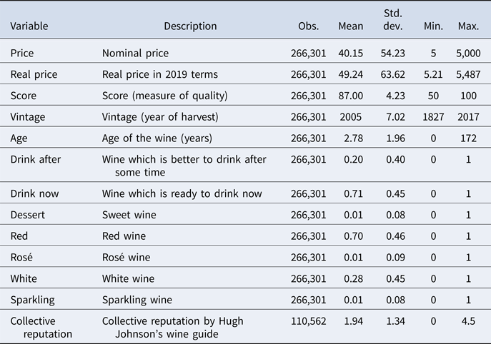
Figure 1 shows the average real price by score value. The average real prices look flat and grow exponentially once the score exceeds 90 points. Regressing the average real prices over a cubic trend provides an R2 equal to 0.86. Figures A1 and A2 show the actual and normal distribution of score values and the natural logarithm of the real price, which will be used in the econometric analysis. A few bottles get less than 70 and more than 98 points.
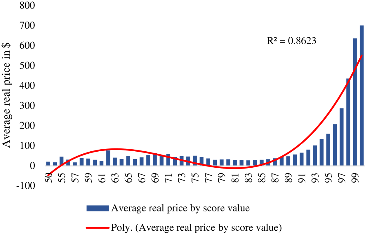
Figure 1. Average real price in $ and quality score.
B. OLS hedonic regressions
The empirical analysis relies on hedonic price regressions. In Table 2, which uses the full database with all countries, the natural logarithm of the real price is regressed over the variables listed in Table 1. Regressions include the vintage year and country dummy variables that are not shown for space reasons but are available upon request. Standard errors are clustered at the country level. We start with a regression that does not include the quality score (Column 1), then add the score in its linear (Column 2), quadratic (Column 3), and cubic (Column 4) specifications, while the last regression uses a set of dummy variables for each score value (Column 5).
Table 2. First stage, determinants of ln of real wine price, all countries
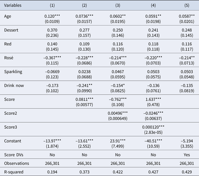
Notes: Regressions include vintage and country DVs. Robust standard errors clustered at the country level in parentheses. Regression in Column (5) uses a set of dummy variables for each score value instead of the linear, quadratic, or cubic functions (results are omitted for reasons of space but are available upon request and are visually represented in Figure 2).
*** p < 0.01, ** p < 0.05, * p < 0.1.
Quality is always strongly significant in all the specifications. The R2 from Column (5), which includes dependent variables (DVs) for all the score values and is the most complete of the regressions proposed, is very close to that of Column (4), which uses a simple cubic function.Footnote 1 The coefficients of the DVs of Column (5) are not shown for reasons of space but are available upon request; Figure 2 plots the values of the coefficients with their confidence intervals. The coefficients of the DVs for scores from 50 to 90 are not statistically different. Above 90 points, the effect of quality on price grows exponentially, and the coefficients of the DVs become gradually higher than those from 50 to 90 points at a 95% significance level.
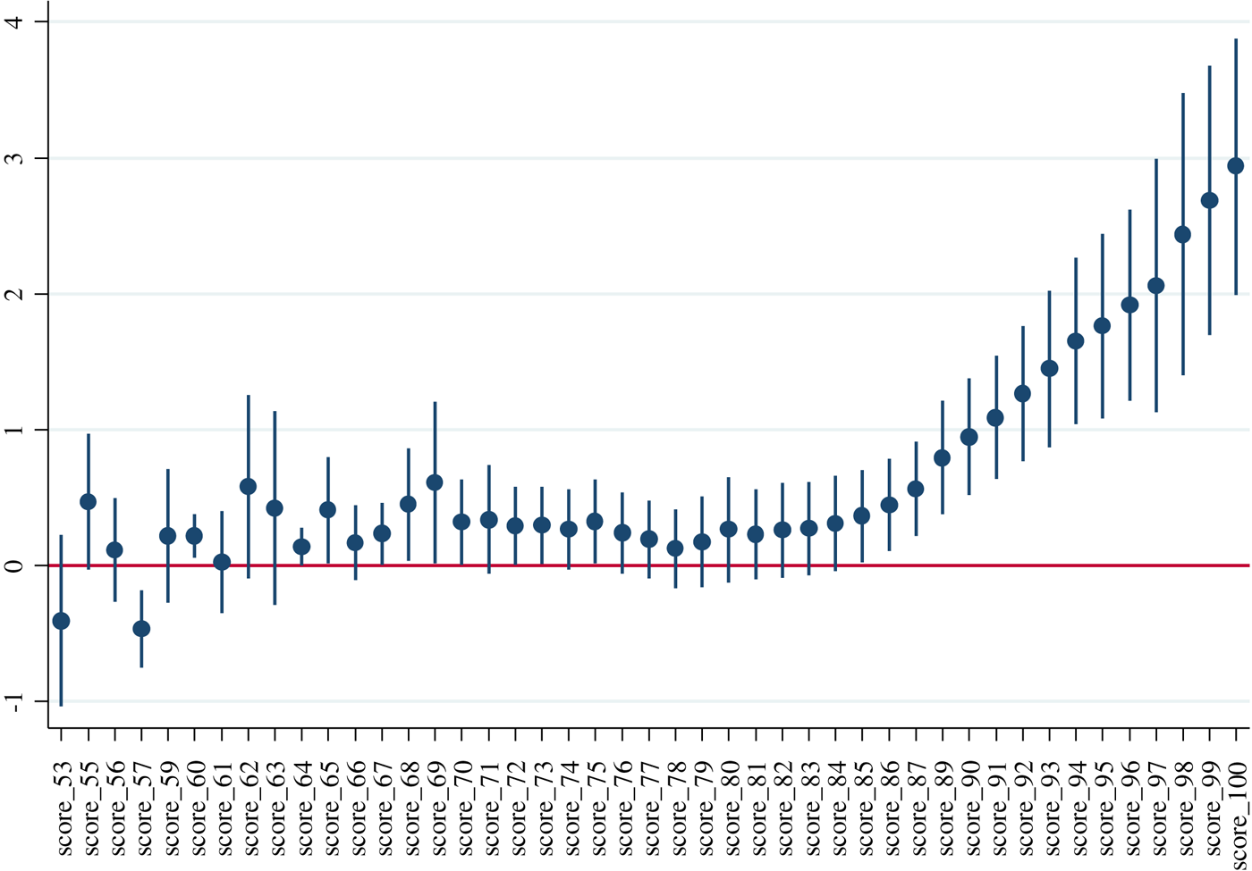
Figure 2. Coefficients and 95% confidence interval of the score DVs.
Note: Results come from regression 5 in Table 2.
In line with previous literature, we find a positive effect of quality on price. However, descriptive statistics and econometric evidence show that the price premium attached to quality is concentrated at the upper end of the distribution. On average, the prices of wines with scores of between 50 and 90 points are statistically not different.
In Table A2 in the Appendix, we repeat regression 4 of Table 2 for each country, and the cubic effect of the score on the ln of price is confirmed for most countries.
C. Heteroskedastic hedonic regressions
In order to describe potential non-linear effects, we adopt a flexible approach: we repeat the hedonic regressions by describing the association with the score, vintage year, and age with restricted cubic splinesFootnote 2 with two internal knots at score = (85, 90), year = (2000, 2011), and age = (5, 10). With the described definition, the design matrix X = (x1, x2, …, xn)T is composed of 26 columns: the constant term, four indicators of dessert, red, rosé, and sparkling wine (reference = White), the “drinknow” indicator, 11 country dummy variables (reference = Argentina), and the three-dimensional splines associated with the score, vintage year, and age. The mean regression model, that is, the standard “linear” model with constant variance largely used in the literature (see Castriota (Reference Castriota2020, Ch. 2) for a review of empirical studies of wine quality and price), was not optimal since it was immediately evident the presence of data heteroskedasticity. Therefore, we considered two alternative solutions: a Normal heteroskedastic model and a quantile regression approach.
The Normal heteroskedastic model is the natural generalization of the standard normal model, that is, the “linear” (mean) regression model. The idea is to describe with a function of the predictors not only the mean but also the variance of a normal distribution, such that Y ~ N(μ(x|β), σ 2(x|θ)). We defined

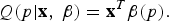
This modeling approach allows for accounting for the presence of heteroskedasticity directly. The conditional mean is given by xT β, which is also the value of the median. Other quantiles, for example the quartiles or the deciles, are defined as Q(p|x, β, θ) = μ(x|β) + σ(x|θ)z(p), where z(.) is the quantile function of a N(0,1) distribution. With our specification of the design matrix, the model had 26 + 26 = 52 parameters, estimated by maximum likelihood. Standard errors were computed by applying standard asymptotic theory, that is, using the square root of the diagonal elements of the negative inverse of the Hessian matrix of the log-likelihood, evaluated at its maximum.
Results in Figure 3a show the predicted mean and median, the quartiles, and the 5th and 95th percentiles of ln(price) as a function of the quality score. All functionals are approximately J-shaped or U-shaped, with all quantiles increasing rapidly for scores above 85. Interestingly, dispersion parameters also show a U-shaped association with the score. In Figure 4, we report the difference between the estimated 95th and 5th percentiles, which achieves a global minimum of approximately 87.5 points.

Figure 3a. Normal heteroskedastic model.
Note: Predicted mean and median, quartiles, and 5th and 95th percentiles of ln(price), as a function of the quality score, as estimated by applying a Normal heteroskedastic model.
In our analysis, we assumed that different types of wines (white, red, rosé, sparkling, and dessert) have the same price-score relationship, up to an additive constant. This assumption may not be plausible and is rejected by the data, where we found a significant interaction (p < 0.0001) between the type of wine and the spline function that describes the price-score association. However, the effect of the score on price is qualitatively the same in all types of wines. The plot in Figure 3b is obtained by applying the Normal heteroskedastic model to each type of wine separately. It can be seen that the functions differ by more than just an additive constant; however, they all show a similar behavior: approximately flat for scores below 80, with a sharper increase for scores between 85 and 90. While this “justifies” our simplifying assumption to pool all wines together, we also understand that a stratified analysis could provide additional useful information; for example, red and white wines show a sharper increase in price than the other three groups.

Figure 3b. Normal heteroskedastic model, by type of wine.
Note: Predicted mean of ln(price), as a function of the quality score, as estimated by applying a Normal heteroskedastic model to each type of wine separately.
Next, in Table A3, we applied the Normal heteroskedastic model using dummy variables for the score in place of spline functions. We report the estimated effects on the conditional mean (β) and log-standard deviation (θ). All the coefficients are highly significant. Results are consistent with those from the spline-based model: the minimum price is found in scores of 75–79, and a sharp increase is found for scores above 90. Moreover, the highest variance around the mean is found at very low and very high scores.
D. Quantile hedonic regressions
In the Normal model, specific quantiles of interest can only be extrapolated using the assumed parametric distribution. An alternative approach is to apply a quantile regression model (e.g., Koenker, Reference Koenker2005). This method avoids global parametric assumptions and allows to directly describe how the p-th quantile depends on the observed predictors, using a regression model of the form
In this model, β(p) is a quantile-dependent vector of regression coefficients. For example, the coefficients that describe the conditional median (p = 0.5) differ from those that characterize the first quartile (p = 0.25) or the 95th percentile (p = 0.95).
Estimation is carried out by minimizing a loss function

where $u = I( y \le {\bf x}^T{\bf \beta }( p) )$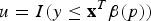 (e.g., Koenker, Reference Koenker2005), while standard errors can be computed by using non-parametric bootstrap. In our analysis, we estimated quantiles of order p = {0.05, 0.25, 0.5, 0.75, 0.95}. Results are illustrated in Figure 4 and are very similar to those obtained with the Normal heteroskedastic model. Some minor differences can be obtained in the estimated 5th and 95th percentiles, especially for low-quality score values. This may suggest that the tails are not well represented by a normal distribution. In Figure 5, we can also see that the difference between the 95th and the 5th percentile found with quantile regression deviates slightly from that obtained using the Normal heteroskedastic model.
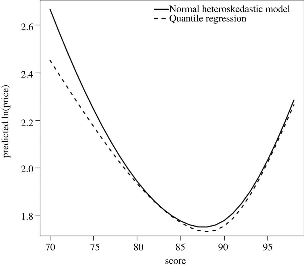
Figure 4. Difference between Q(0.95) and Q(0.05).
Note: Estimated difference between the 95th and the 5th percentile of ln(price), expressed as a function of the quality score. Continuous line: Normal heteroskedastic model. Dashed line: quantile regression model.
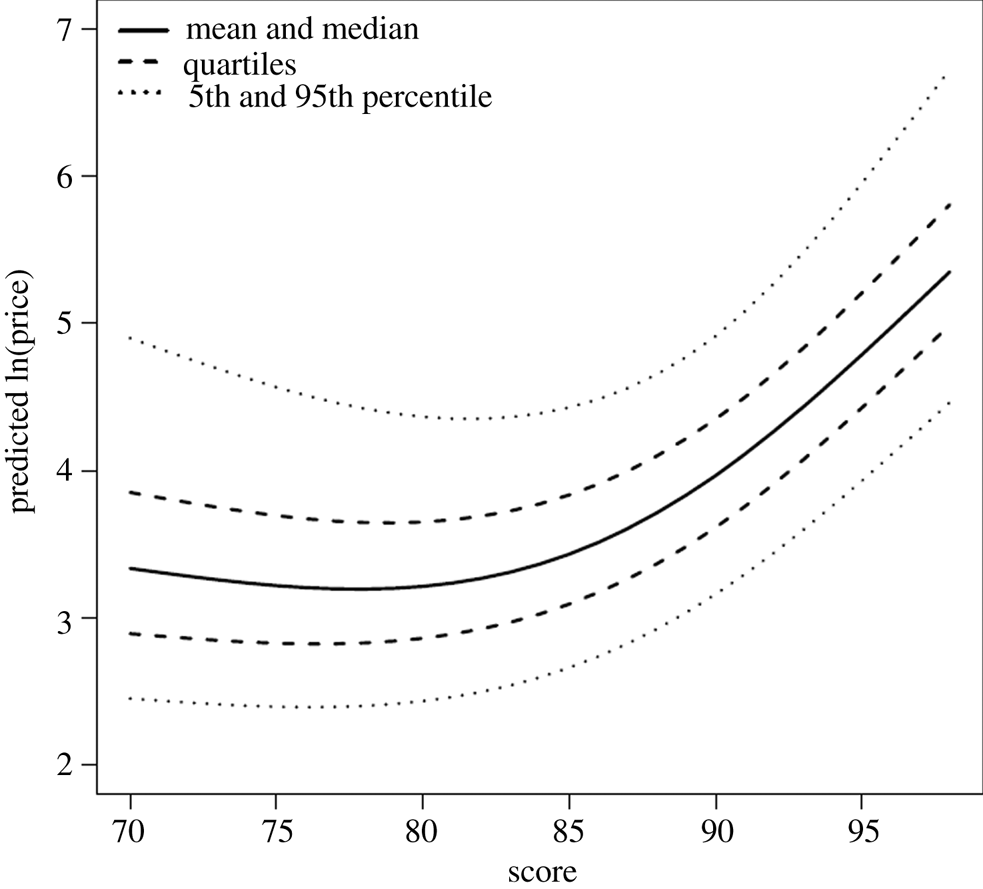
Figure 5. Quantile regression model.
Note: Predicted median, quartiles, and 5th and 95th percentiles of ln(price), as a function of the quality score, as estimated by applying a Quantile regression model.
V. Conclusions
Quality is commonly considered the most important driver of wine prices. An extensive literature has shown a positive link between the two variables. This work provides new evidence using an extensive database of 266,301 bottles from 12 countries sold in the United States and rated by WS. The positive link between quality and price achieved is confirmed. However, the focus on “superstar” wines deserves more attention. In fact, whereas wines with quality scores between 50 and 90 points (in a 50–100 range) have prices that are statistically not different, above 90 points, prices grow exponentially and become statistically different. Furthermore, the dispersion of the residuals of hedonic regressions is U-shaped with respect to quality.
While many wine producers pursue quality excellence to obtain greater recognition in the market and a premium on the retail price, the significant effect of wine quality on prices can only be achieved with outstanding scores. Hence, it seems reasonable to wonder whether the potential benefits in terms of price are worth the efforts and costs required to achieve an excellent quality product. This research suggests that a strategy to attain a higher price based on quality can be effective when the aim is to produce outstanding wine, that is, with a quality score higher than 90, beyond which prices increase considerably.
On the other hand, wines with a quality score above 90 also show a significantly higher price dispersion, suggesting that while producing wines of excellent quality can bring significant benefits in terms of price, at the same time, it also increases the uncertainty about the results. Pursuing an outstanding quality is a very ambitious and potentially profitable strategy, but it also exposes us to greater risks due to price dispersion.
Even though our research is targeted at hedonic modelers, we believe it is important to mention the concerns about the potential benefits in terms of price from pursuing qualitative excellence. In order to provide definite policy suggestions, however, we should have information on a number of additional domains, such as firm investments and cost functions. With this respect, we acknowledge the limits of our work. Nevertheless, since the link between the quality of wines produced and firm profitability is crucial for wineries but unexplored by researchers, future investigations should focus on this topic.
Acknowledgments
The authors wish to thank (without implicating) Angelo Zago for the helpful comments in the early stages of this research and the reviewers and editors for their comments and constructive remarks.
Appendix
Table A1. Sample distribution by country
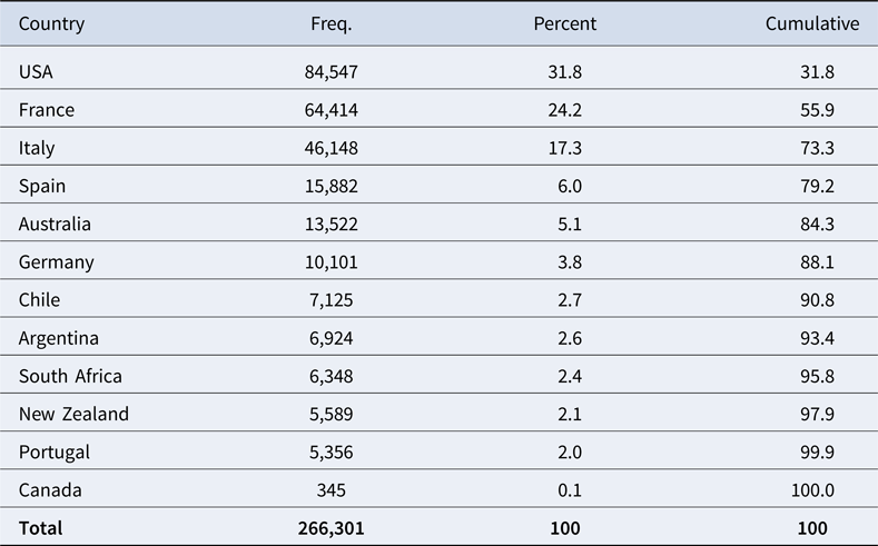
Table A2. First stage, determinants of ln of real wine price, by country
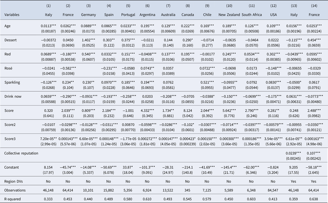
Table A3. Normal heteroskedastic model using dummy variables for the score, in place of spline functions.
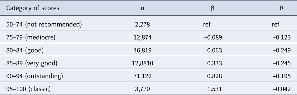
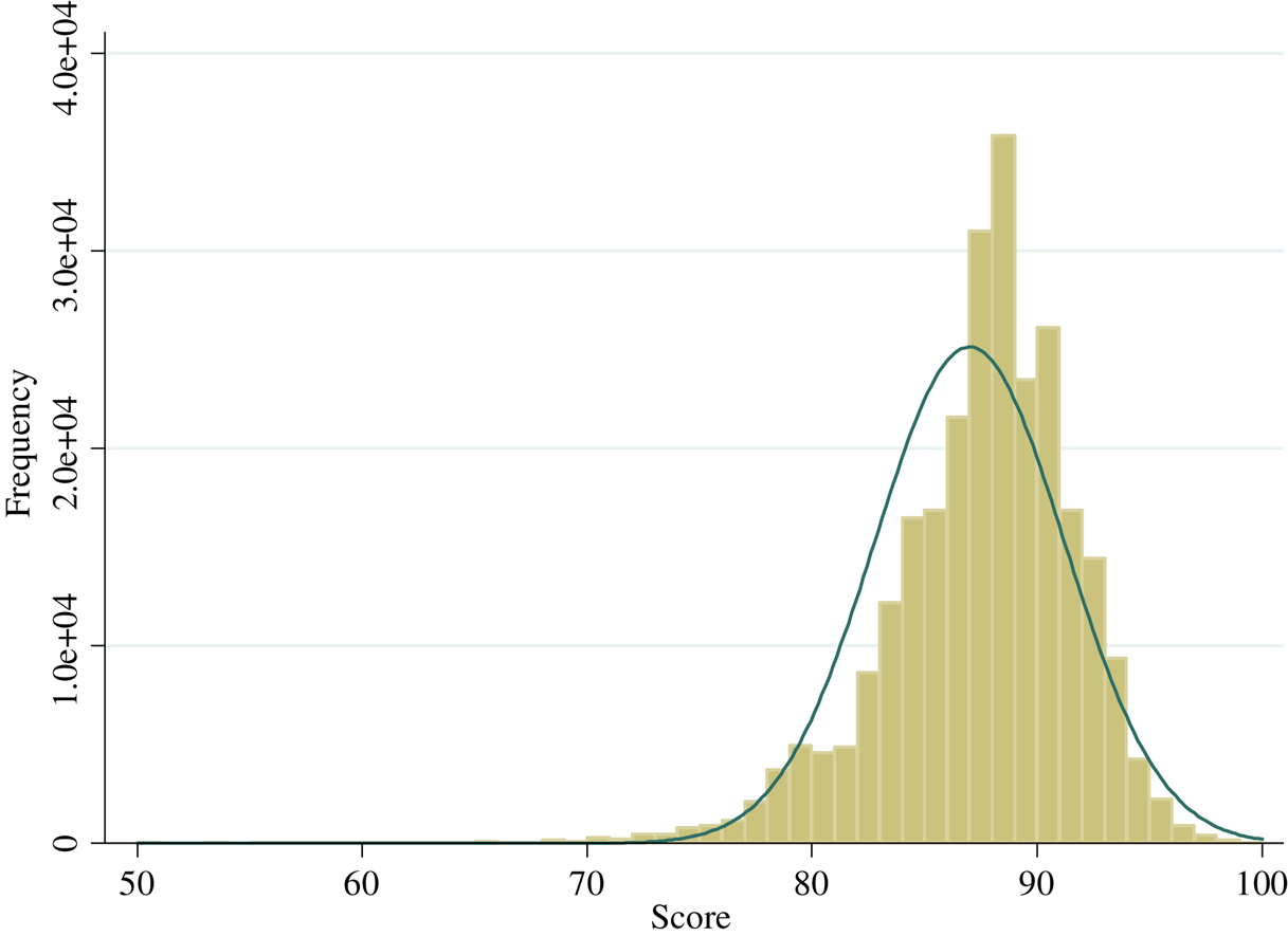
Figure A1. Distribution of score values.
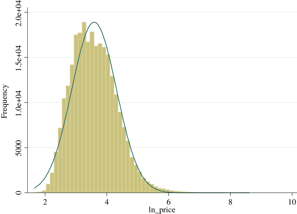
Figure A2. Distribution of log of real price.


 Open access