


1. Introduction
Natural flyers exhibit remarkable flight performance in the low-Reynolds-number regime and attract wide attention for their potential as the inspiration for novel unmanned aerial systems. Natural flapping flight utilizing unsteady aerodynamic effects enables unconventional means of aerodynamic force generation by its sophisticated flapping kinematics and wing morphology (Shyy et al. Reference Shyy, Aono, Kang and Liu2013, Reference Shyy, Kang, Chirarattananon, Ravi and Liu2016; Hassanalian & Abdelkefi Reference Hassanalian and Abdelkefi2017). As one of the most successful aerial predators on Earth, dragonflies have survived and evolved for millions of years (Combes et al. Reference Combes, Rundle, Iwasaki and Crall2012). Unlike wings of birds or bats, the dragonfly wing is a complex mechanical structure without muscle or bone, and the wing morphology of a dragonfly is characterized by multiscale wings, such as the resilin, wing corrugation, nodus and pterostigma, which greatly affect the structural dynamics of the flapping wings and, hence, flight performance (Rajabi & Gorb Reference Rajabi and Gorb2020; Wootton Reference Wootton2020).
Dragonflies are physiologically capable of controlling any of their wings individually, unlike most other quad-winged insects where stronger internal muscular linking is present between the wings (Neville Reference Neville1960; Büsse, Helmker & Hörnschemeyer Reference Büsse, Helmker and Hörnschemeyer2015; Bäumler, Gorb & Büsse Reference Bäumler, Gorb and Büsse2018). Studies have shown that a small change in the flapping motion of wings may lead to a large change in aerodynamic force generation (Sane & Dickinson Reference Sane and Dickinson2001; Altshuler et al. Reference Altshuler, Dickson, Vance, Roberts and Dickinson2005; Shyy et al. Reference Shyy, Aono, Chimakurthi, Trizila and Kang2010). Recently, it has been shown that for a flapping winged system not only the range and timing (Lee, Jang & Lee Reference Lee, Jang and Lee2020) of kinematic motions but the complex waveforms can influence the leading-edge vortex (LEV) formation and added mass effects (Bhat et al. Reference Bhat, Zhao, Sheridan, Hourigan and Thompson2020; Lee et al. Reference Lee, Jang and Lee2020). In a numerical study with optimization function, Kamisawa and Isogai showed that from hovering to fast forward flight to keep the necessary power minimal, the stroke plane angle should gradually increase (from about 8° to 88°) together with the wing phasing (from about 30° to 90° hindwing lead), while the rate of twist decreases, and the flapping amplitude of the forewing and the hindwing varies as 30°–60° and 20°–40° respectively (Kamisawa & Isogai Reference Kamisawa and Isogai2008). Dragonflies in actual flight, however, can deviate substantially from the optimal flapping kinematics presented in the above study due to physiological, situational and environmental conditions that were not considered in the optimization model. Phasing of the flapping positional angle of the forewings and hindwings in dragonflies has been comprehensively studied to reveal the unique aerodynamic features of tandem-winged flapping wing flight (Maybury & Lehmann Reference Maybury and Lehmann2004; Usherwood & Lehmann Reference Usherwood and Lehmann2008; Broering, Lian & Henshaw Reference Broering, Lian and Henshaw2012; Hu & Deng Reference Hu and Deng2014; Xie & Huang Reference Xie and Huang2015; Hefler, Qiu & Shyy Reference Hefler, Qiu and Shyy2018; Nagai, Fujita & Murozono Reference Nagai, Fujita and Murozono2019). In-phase flapping is usually observed when dragonflies do quick, demanding flight manoeuvres, while out-of-phase flapping is adopted during hovering and steady free flight (Norberg Reference Norberg1975; Azuma & Watanabe Reference Azuma and Watanabe1988; Rüppel Reference Rüppel1989; Wakeling & Ellington Reference Wakeling and Ellington1997). Besides varying the flapping positional angle of each wing, a dragonfly is also able to actively pitch its wing about the spanwise axis as a tool for setting the local angle of attack of its wings (Liu et al. Reference Liu, Hefler, Shyy and Qiu2021b). Asymmetric pitching is adopted by dragonflies, which leads to large attack angle at mid-downstroke and small attack angle at mid-upstroke producing larger vertical force with less aerodynamic power (Park & Choi Reference Park and Choi2012). The local angle of attack can strongly influence the unsteady lift-generating mechanisms of flapping flight (Thomas et al. Reference Thomas, Taylor, Srygley, Nudds and Bomphrey2004; Bomphrey et al. Reference Bomphrey, Nakata, Henningsson and Lin2016). It was also shown that the synchronized phasing and pitching of the wings in hovering flight can help dragonflies overcome the adverse effects of root vortex interaction with LEV formation (Zou, Lai & Yang Reference Zou, Lai and Yang2019). A previous study based on the flight of a living dragonfly using smoke visualization in a wind tunnel shows that the effective angle of attack of the flapping wing played a primary role in the formation, attachment and shedding of the LEV (Thomas et al. Reference Thomas, Taylor, Srygley, Nudds and Bomphrey2004). The control of flapping kinematic parameters results in complex vortex interactions between the wings, capture and utilization of wake elements as well as downwash effects along the wingspan that strongly influence the aerodynamic performance of dragonflies (Broering et al. Reference Broering, Lian and Henshaw2012; Hu & Deng Reference Hu and Deng2014; Zheng, Wu & Tang Reference Zheng, Wu and Tang2016; Hefler et al. Reference Hefler, Qiu and Shyy2018, Reference Hefler, Noda, Qiu and Shyy2020). Free flight kinematics in turning manoeuvres were measured and evaluated numerically by Li & Dong (Reference Li and Dong2017), showing how dragonflies control the inner and outer wings to facilitate steep turns. The wings towards the axis of the turn sweep slower with a higher angle of attack during the downstroke while sweeping faster with a lower angle of attack during the upstroke than the outer wings resulting in higher drag on the inner side especially during downstroke and a thrust boost on the outer side during upstroke (Li & Dong Reference Li and Dong2017). Recently Liu et al. (Reference Liu, Hefler, Shyy and Qiu2021b) studied the change of the flapping kinematics of a live tethered dragonfly resulting in two distinct flight modes: a normal (forward) flight mode and an escape-like manoeuvring flight mode. Escape flight mode, or escape flapping kinematics, is primarily a manoeuvring flight behaviour for an attempted quick take-off or ‘mid-air jump’ characterized by large transient lift peaks and a downward diverted compressed wake (Somps & Luttges Reference Somps and Luttges1986; Yates Reference Yates1986; Reavis & Luttges Reference Reavis and Luttges1988; Liu et al. Reference Liu, Hefler, Shyy and Qiu2021b). Liu et al. (Reference Liu, Hefler, Shyy and Qiu2021b) show that the dragonfly does not alter its flapping frequency substantially for facilitating the escape flight but controls the angle of attack of its wings by the change of the stroke plane angle and the pitching, while adjusting the stroke amplitude of the wings and their phasing are hypothesized to increase the propulsive efficiency (Liu et al. Reference Liu, Hefler, Shyy and Qiu2021b). The experimental methodology, however, does not allow the independent variation of these kinematic parameters, so it is not yet well understood as to how each of these changes take part in flight control or whether there is any synergistic effect between them.
This work employs a high-fidelity numerical model to further explore the effect and importance of changing wing kinematics for flight control. Unlike in real dragonflies, the numerical simulation allows for a parametric study of the kinematics in isolation and in certain combinations, while other parameters are kept unchanged. The results can provide insight into how individual kinematic parameters may play a more or a less important role in various flight missions of a micro air vehicle to help simplify its wing actuation mechanics.
2. Experimental and numerical set-up
2.1. Experimental measurement of the wing kinematics and flow fields of a live dragonfly in distinct flight modes
In a previous work (Liu et al. Reference Liu, Hefler, Shyy and Qiu2021b), we measured the wing kinematics and flow fields by the flapping wings of a live tethered dragonfly of the species wandering glider (Pantala flavescens). The results regarding two distinct flapping behaviours of the dragonfly, namely the kinematics of a normal (forward) flight mode and an escape flight mode, are used in this work to define the parameter space of a systematic numerical study. For this reason, the experimental set-up of the kinematics measurement is briefly described first. More details can be found in Liu et al. (Reference Liu, Hefler, Shyy and Qiu2021b).
A live dragonfly was glued to a glass plate at its thorax without restricting the actuation of the wings, head and abdomen in any way. A time-resolved particle image velocimetry (PIV) set-up (Lavision GmbH) was used to measure the flow field and record the wing kinematics (Hefler et al. Reference Hefler, Qiu and Shyy2018; Liu et al. Reference Liu, Hefler, Shyy and Qiu2021b). Tethering the specimen ensured an adequate field of view in the PIV measurement and reduced the effect of strong light reflection from the wings and the body. The kinematic parameters of the flapping wings were calculated using the known distance between the pterostigma and the wing root of the specimen along with the projected positions of the pterostigma (a natural landmark near the tip of each wing) and the wing root from the recorded PIV frames. During the PIV experiment, a given cross-section of the wing was illuminated by a laser sheet. The pitching angle was calculated from the positions of the leading edge and the trailing edge of the illuminated cross-section of the wing in the PIV frames. We measured the pitching angle close to the wing root (5 mm from the rotational joint of the dragonfly) to decouple the effect of passive wing twisting due to wing flexibility. As the wings camber along the chord, the pitching angle is defined as the angle between the line connecting the trailing edge to the leading edge and the body line, which is horizontal in our set-up (figure 1). The pitching angle is positive when the leading edge is below the trailing edge (during downstroke). The positions of the pterostigma, the leading edge and the trailing edge of the wings on the image frames were manually traced. The derived parameters are averaged over four flapping cycles to describe the wing kinematics.

Figure 1. The definition of the kinematic and geometric angles of a flying dragonfly used in the computational model. The stroke plane is defined as the x′–y′ plane. The stroke plane angle is β. The wing positional angle is φ. The pitching angle is α.
Dragonflies seem not to vary the flapping frequency under different flight modes (Liu et al. Reference Liu, Hefler, Shyy and Qiu2021b), so we focus on the other kinematic parameters. We set the flapping frequency at 28.2 Hz (Liu et al. Reference Liu, Hefler, Shyy and Qiu2021b) for all cases and investigate the interplay between wing phasing, flapping amplitude, wing angles and aerodynamics. Table 1 summarizes the kinematic parameters used in this work.
Table 1. Parameters used in the numerical model and the cases studied (the average value of seven specimens in normal or in escape flight was used where it is indicated).

2.2. Numerical model
For the analysis of the flow field around the dragonfly model, we used a computational fluid dynamics solver based on a finite volume method and a Navier–Stokes solver for a multi-blocked, overset-grid system (Liu & Kawachi Reference Liu and Kawachi1998; Liu Reference Liu2009). The computational domain, the body orientation and the flapping wing kinematics are described with the help of global (X–Y–Z, with origin at the corner of the computational domain) and wing-fixed (x′–y′–z′, with origin at the root of each wing) coordinate systems (figure 1). The transformations among these three coordinate systems are easy to establish to facilitate the dynamic regridding of the computational domain (Liu Reference Liu2009). The wing-fixed coordinate system is rotated in the stroke plane to provide a convenient way to describe the change of the positional angle (φ), the pitching angle (α) and the deviation angle (χ) (figure 1).
The stroke plane is the plane in which the wing is flapping. The positional angle (φ) defines the wing's position within the stroke plane. The origin of the positional angle is the wing pivot. The positional angle is zero when the wing's spanwise axis is parallel to the principal plane of the dragonfly body sideways. The pitching angle (α) defines the wing chord's pitching around the spanwise axis. The deviation angle (χ) defines the wing motion out of the stroke plane during a flapping cycle. The stroke plane angle (β) is the angle between the stroke plane and the horizontal axis in the global coordinate system (figure 1). The experimentally measured flapping kinematics of the dragonfly can be well described with two angles around the wing pivot, as the deviation angle (χ) is negligible.
Natural insect wings are flexible, but implementing fully coupled fluid–structure interaction (FSI) under dynamic three-dimensional loading would be computationally expensive using advanced dynamic regridding of the computational domain and necessitate a precise definition of the material structural properties of the dragonfly wings. Rigid wing modelling, on the other hand, would be an oversimplification. With the help of high-speed videos, we observed that the general wing morphology does not change noticeably during the tethered normal and the escape flight modes. Our assumption is that during free flight, the general morphology would also not change substantially. The morphology prescribed in our model (without FSI) is not a flexible wing model in a traditional interpretation, but it is more realistic than the idealized rigid wing model would be, and the computation is less demanding than using a FSI scheme. By adopting one specific general wing morphology and scaling it only by the time in one flapping cycle, the amount of the wing deformation including spanwise bending, twist and camber is the same in all cases and the results are not affected by morphological changes rather than the change of flapping kinematic parameters. It should be noted here that the wing kinematics, the wing deformations and the aerodynamic forces are strongly coupled in dragonflies and using the same wing deformation in all cases may lead to different results from those of actual flight. The morphological model of the wings with prescribed deformations was constructed based on the measured dynamic deformation of the wings of a free-flying dragonfly in steady forward flight, which closely resembles the normal flight mode. This measurement involved painting markers on the wings of the dragonfly (figure 2a) that was then released to fly freely in a flight chamber while being recorded from multiple viewing angles (Hefler et al. Reference Hefler, Noda, Qiu and Shyy2020). The markers were manually traced on the recorded frames of high-speed videos (figure 2b), allowing for a direct linear transformation to the computational domain according to a preset calibration matrix (Hedrick Reference Hedrick2008). We traced three flapping cycles and selected the cycle that provided the best continuity for the numerical model (‘dragonfly 2 – flight 2’ in Hefler et al. (Reference Hefler, Noda, Qiu and Shyy2020)). The cycle-to-cycle variation of the flapping positional angle was reasonably small in the selected flight (Hefler et al. Reference Hefler, Noda, Qiu and Shyy2020). A surface fitted on the traced markers (figure 2c) was used to define the prescribed deformations of the wings in the numerical simulation. The dimensions of the forewings and hindwings are given in table 1. This dynamic shape conformed to the actual kinematic parameter range measured experimentally for the cases studied (table 1) in this work. To ensure good continuity of the kinematic parameters in the simulation, fitted curves were adopted by using the fourth order of Fourier series for the periodic computation as described in Liu (Reference Liu2009). Further details of the morphological measurement can be found in Hefler et al. (Reference Hefler, Noda, Qiu and Shyy2020).

Figure 2. Steps of the morphological measurement of the flexible wings of a free-flying dragonfly. (a) Markers painted on the live specimen; (b) tracking the markers on high-speed video frames; (c) fitting a surface on the transformed coordinates of the markers.
The computational domain was an 8RFW × 8RFW × 8RFW (where RFW is the wing length of the forewing) sized Cartesian grid (figure 3) in which the body grid and the two fore- and hindwing grids (flyer blocks) are immersed. The Cartesian grid has two subregions: the clustering region, which has small, uniform grid spacing and the global cluster, which is gradually refined towards the centre of the computational domain. The uniform grid spacing is set to be 0.15CFW (where CFW is the mean chord length of the forewing) in the model. The outer boundaries of the flyer blocks are immersed in the clustering region to prevent loss of accuracy due to the interpolation between the global block and flyer blocks. Note that the wing blocks have an outside boundary of CFW/2 or CHW/2 from each wing surface respectively (where CHW is the mean chord length of the hindwing). The numbers of grid points in i × j × k are the following: the global grid is 117 × 121 × 117; the body grid is 35 × 35 × 9; the two fore- and hindwing grids are 37 × 37 × 17. The wing grids were clustered along the edges of the wing for higher resolution in the regions where shear flow is expected. The averaged grid size on the forewing surface is approximately 0.056CFW and 0.15CFW in the chord and span direction. The averaged grid size on the hindwing is chosen similarly to be 0.056CHW and 0.15CHW in the chord and span direction respectively. A uniform thickness (0.5 % of CFW or CHW) is taken for the wing but with elliptic smoothing along the edges. The dragonfly model is fixed in the domain, and the head, thorax and abdomen ensemble is treated as one rigid body. The dragonfly is fixed in the X–Y plane with its body parallel to the X axis. The convergence of the flow field was ensured with this value as described in Appendix D (tables 6 and 7, and figure 22).

Figure 3. The computational domains: (a) global grid block and (b) grids of a dragonfly body and wings.
The governing equations of the numerical solver are the three-dimensional, incompressible, unsteady Navier–Stokes equations written in strong conservation form for mass and momentum (Liu & Kawachi Reference Liu and Kawachi1998; Liu Reference Liu2009; Hefler et al. Reference Hefler, Noda, Qiu and Shyy2020). The artificial compressibility method is used by adding a pseudo time derivative of pressure to the equation of continuity. For an arbitrary deformable control volume V(t), the non-dimensional governing equations are
 \begin{align} \int_{V(t)} {\left( {\frac{{\partial \boldsymbol{Q}}}{{\partial t}} + \frac{{\partial \boldsymbol{q}}}{{\partial \tau }}} \right)\textrm{d}V} + \int_{V(t)} {\left( {\frac{{\partial \boldsymbol{F}}}{{\partial x}} + \frac{{\partial \boldsymbol{G}}}{{\partial y}} + \frac{{\partial \boldsymbol{H}}}{{\partial z}} + \frac{{\partial {\boldsymbol{F}_v}}}{{\partial x}} + \frac{{\partial {\boldsymbol{G}_v}}}{{\partial y}} + \frac{{\partial {\boldsymbol{H}_v}}}{{\partial z}}} \right)\textrm{d}V} = 0, \end{align}
where bold type is used to denote matrices as
 \begin{align}\boldsymbol{Q} &= \left[ {\begin{array}{@{}c@{}} u\\ v\\ w\\ 0 \end{array}} \right],\quad \boldsymbol{q} = \left[{\begin{array}{@{}c@{}} u\\ v\\ w\\ p \end{array}} \right],\quad \boldsymbol{F} = \left[{\begin{array}{@{}c@{}} {{u^2} + p}\\ {uv}\\ {uw}\\ {\lambda u} \end{array}} \right],\nonumber\\ \boldsymbol{G} &= \left[ {\begin{array}{@{}c@{}} {vu}\\ {{v^2} + p}\\ {vw}\\ {\lambda v} \end{array}} \right],\quad \boldsymbol{H} = \left[ {\begin{array}{@{}c@{}} {wu}\\ {wv}\\ {{w^2} + p}\\ {\lambda w} \end{array}} \right],\end{align}
 \begin{align}{\boldsymbol{F}_{\boldsymbol{v}}} &={-} \frac{1}{{Re}}\left[ {\begin{array}{@{}c@{}} {2{u_x}}\\ {{u_y} + {v_x}}\\ {{u_z} + {w_x}}\\ 0 \end{array}} \right],\quad {\boldsymbol{G}_{\boldsymbol{v}}} ={-} \frac{1}{{Re}}\left[{\begin{array}{@{}c@{}} {{v_{x + }}{u_y}}\\ {2{v_x}}\\ {{v_z} + {w_y}}\\ 0 \end{array}} \right],\nonumber\\ {\boldsymbol{H}_{\boldsymbol{v}}} &={-} \frac{1}{{Re}}\left[{\begin{array}{@{}c@{}} {{w_{x + }}{u_z}}\\ {{w_{y + }}{v_z}}\\ {2{w_z}}\\ 0 \end{array}} \right].\end{align}
In the above, λ is the pseudo-compressibility coefficient; p is pressure; u, v and w are velocity components in the Cartesian coordinate system X, Y and Z; t denotes physical time, while τ is pseudo-time; and Re is the Reynolds number. The term q associated with the pseudo-time is designed for an inter-iteration at each physical time step, which will vanish when the divergence of velocity is driven to zero to satisfy the equation of continuity. Reynolds number is defined as
 \begin{equation}Re = \frac{{{U_{ref}}{L_{ref}}}}{\nu },\end{equation}
where Uref is a reference velocity, Lref is a reference length and ν is the kinematic viscosity of air. The forewing mean chord length is used as the reference length. The mean wingtip velocity of the forewing is used as reference velocity: Uref = Utip = ωR, where R is the span length and ω is the mean angular velocity of the flapping wing (ω = 2 $\varPhi$f, where $\varPhi$ is the wing positional angle amplitude and f is the flapping frequency). The resulting reference velocities are 3.27 m s−1 in cases 1, 3, 4, 5 and 2.71 m s−1 in case 2. The Reynolds number in cases 1 and 3–5 is 1732 for the forewing and 2408 for the hindwing, while it is 1435 for the forewing and 1914 for the hindwing in case 2. All the reference velocities are much less than 0.3a (a is the speed of sound), and all the Reynolds numbers are in the laminar flow regime. Therefore, the incompressibility assumption is reasonable, and no turbulence modelling is required; thus, the computation is done in the laminar flow regime.
For the time integration, the Padè scheme is employed as
 \begin{equation}\; \frac{\partial }{{\partial t}} = \left( {\frac{1}{{\Delta t}}} \right)\left( {\frac{\Delta }{{1 + \Delta \theta }}} \right),\end{equation}
where parameter θ is taken to be 0.5 for the implicit Euler scheme with second-order accuracy in time; Δt is the time increment; and Δ is the differencing operator:
 \begin{equation}\mathrm{\Delta }\; = {\boldsymbol{q}^{(n + 1)}} - {\boldsymbol{q}^{(n)}}.\end{equation}
The Navier–Stokes equation (2.1) can be reformed in terms of the semi-discrete form, where (i,j,k) denote the cell index, such that
 \begin{equation}\frac{\partial }{{\partial t}}{[V\boldsymbol{Q}]_{ijk}} + {\boldsymbol{R}_{ijk}} + {V_{ijk}}\left( {{\boldsymbol{a}_0} + \frac{{\partial \boldsymbol{q}}}{{\partial \tau }}} \right)_{ijk} = 0,\end{equation}
where
 \begin{align} {\boldsymbol{R}_{ijk}} & = {(\hat{\boldsymbol{F}} + {{\hat{\boldsymbol{F}}}_v})_{i + 1/2,j,k}} - {(\hat{\boldsymbol{F}} + {{\hat{\boldsymbol{F}}}_v})_{i - 1/2,j,k}} + {(\hat{\boldsymbol{G}} + {{\hat{\boldsymbol{G}}}_v})_{i,j + 1/2,k}} - {(\hat{\boldsymbol{G}} + {{\hat{\boldsymbol{G}}}_v})_{i,j - 1/2,k}}\nonumber\\ & \quad + {(\hat{\boldsymbol{H}} + {{\hat{\boldsymbol{H}}}_v})_{i,j,k + 1/2}} - {(\hat{\boldsymbol{H}} + {{\hat{\boldsymbol{H}}}_v})_{i,j,k - 1/2}} \end{align}
and
 \begin{gather}\textrm{e}\textrm{.g}\textrm{.}\;\; \hat{\boldsymbol{F}} + {\hat{\boldsymbol{F}}_v} = (\boldsymbol{f} - \boldsymbol{Q}{\boldsymbol{u}_{\boldsymbol{g}}})\boldsymbol{\cdot }\boldsymbol{S}_n^\xi ,\end{gather}
 \begin{gather}\boldsymbol{S}_n^\xi = [S_{nx}^\xi ,S_{ny}^\xi ,S_{nz}^\xi ].\end{gather}
The term  ${\boldsymbol{a}_0}$ denotes the acceleration of the body in the translational direction, which is explicitly derived from the velocity. The term ${V_{ijk}}$ is the volume of the cell (i,j,k) and ${\boldsymbol{u}_{\boldsymbol{g}}}$ is the local velocity of the moving cell surface. The term $\boldsymbol{S}_n^\xi $ stands for the areas of the cell faces, e.g. $\boldsymbol{S}_n^\xi $ in $\xi $ direction in computational space. The equation can be discretized by replacing the time-related term with (2.5), such that
 \begin{align}\mathrm{\Delta (}V\boldsymbol{Q})_{ijk}^{(n)} + \mathrm{\Delta }\theta \mathrm{\Delta }t{\left[ {{\boldsymbol{R}_{ijk}} + {V_{ijk}}{{\left( {{\boldsymbol{a}_0} + \frac{{\partial \boldsymbol{q}}}{{\partial \tau }}} \right)}_{ijk}}} \right]^{(n)}} ={-} \mathrm{\Delta}{t}{\left[ {{\boldsymbol{R}_{ijk}} + {V_{ijk}}{{\left( {{\boldsymbol{a}_0} + \frac{{\partial \boldsymbol{q}}}{{\partial \tau }}} \right)}_{ijk}}} \right]^{(n)}}.\end{align}
Further details can be found in Liu & Kawachi (Reference Liu and Kawachi1998).
On the body surface, the no-slip condition is used for the velocity components. To incorporate the dynamic effect due to the acceleration of the oscillating body (moving and/or deforming body surface), the pressure gradient at the surface stencils is derived from the local momentum equation, such that
 \begin{gather}(u,v,w) = ({u_{body}},{v_{body}},{w_{body}}),\end{gather}
 \begin{gather}\frac{{\partial p}}{{\partial \boldsymbol{n}}} ={-} {\boldsymbol{a}_0}\boldsymbol{\cdot }\boldsymbol{n},\end{gather}
where the velocity  $({u_{body}},{v_{body}},{w_{body}})$ and the acceleration ${\boldsymbol{a}_0}$ on the solid wall are evaluated and updated using the updated grids on the body surface at each time step. The boundary conditions of the background grid for the velocity and the pressure are given as: (1) at upstream the velocity is the inflow while pressure is set to zero, and (2) at downstream zero-gradient condition is taken for both velocity and pressure. Escape and normal flight would involve different free-stream flows from different directions. However, most of our studied cases are created by using a mix of parameters from these two flight modes creating hypothetical cases for which determining a preset realistic inflow was not possible. Under different flapping modes, the flight speed as well as the kinematics of the wing movement change the angle of attack which was found to be an important factor influencing the flight dynamics. On the other hand, the flapping frequency of the wings of a dragonfly is so high that wing kinematics of the flapping cycle characterize the local angle of attack and vortex shedding rather than the flight speed (Taylor, Nudds & Thomas Reference Taylor, Nudds and Thomas2003). For these reasons, we chose to evaluate the effect of the changing of the kinematic parameters isolated from free flow and simulate the reference escape and normal flight modes under the same condition. As a result, the inflow is set to zero in this study.
When we solve the Navier–Stokes equations for a wing block, the aerodynamic forces exerted on the wing are evaluated by a sum of inviscid and viscous flux over the wing surface as
 \begin{equation}{\boldsymbol{F}_{aero}}({F_x},{F_y},{F_z}) ={-} \sum\limits_i^n {(\boldsymbol{Flux}_{invis} + \boldsymbol{Flux}_{vis})} ,\end{equation}
where n denotes the cell number on the surface of the wing. Note that this method could minimize the numerical error during the integration rather than directly integrating the velocity gradient-based stresses and the pressures over the wing surface (Liu & Kawachi Reference Liu and Kawachi1998).
For the convergence of the flow fields, we conducted five cycles of simulation, and the results are derived from the final flapping cycle (see table 3 and figure 20 in Appendix B). In addition, to observe the influence of the time step, the domain size and the grid resolution on the computational results, we conducted a sensitive study. The time step for the computation is 1500 steps for one flapping cycle corresponding to about 2.36 × 10⁻³ s, and the convergence of the flow field was ensured with this value as described in Appendix C (tables 4 and 5, and figure 21). The validity of the numerical model for the study of the unsteady fluid dynamics involved in insect flight has been shown in previous works (Hefler et al. Reference Hefler, Noda, Qiu and Shyy2020, Reference Hefler, Kang, Qiu and Shyy2021).
3. Results and discussion
3.1. Aerodynamic forces
The aerodynamic forces are presented considering both the right and left wings. For total aerodynamic force calculations, we consider only the wings and forces acting on the body of the dragonfly are neglected. The total force (F Σ) is calculated as the vector sum of lift (FL) and thrust (FT) forces. Lift is the vertical component while thrust is the horizontal component of the total force. Table 2 summarizes the cycle-averaged aerodynamic forces, power (P) and efficiencies in the reference cases (cases 1 and 2). The cycle-averaged force coefficients (CL, CT, CΣ), power coefficients (CP) and the ratio of the total force and power coefficients (CΣ/CP) for all the cases studied are also listed in table 2. The ratio of the cycle-averaged total force coefficient to the power coefficient is used to express the overall efficiency in a non-dimensional form. Non-dimensional values can help in the interpretation of the results in the context of previous works related to flapping wing flight; however, to avoid the mismatch of the values in the reference cases (cases 1 and 2) where the reference velocities (mean wingtip velocity of the forewing) were different, the use of dimensional values is necessary. For the same reason, in cases 1 and 2, the cycle-averaged aerodynamic force-to-power ratio (FΣ/P) is used to calculate the efficiency (Zheng, Hedrick & Mittal Reference Zheng, Hedrick and Mittal2013). The aerodynamic power is the power imparted to the air by wings during a flapping cycle. If the flyer flaps symmetrically between the right and left wings, the power due to the lateral velocities (Y component; figure 3a) is zero as can be seen in (3.1). The aerodynamic power imparted to the air by each wing is defined as (Zheng et al. Reference Zheng, Hedrick and Mittal2013)
 \begin{equation}P = \; - \sum\limits_i^N {({\boldsymbol{F}_{aero,i}}\boldsymbol{\cdot }{\boldsymbol{v}_{surf,i}})} ,\end{equation}
where N denotes the number of the elements on the surface of each wing;  ${\boldsymbol{F}_{aero}}$ is aerodynamic forces acting on each element; and ${\boldsymbol{v}_{surf}}$ is the corresponding velocity of each element. The aerodynamic power of the body is not considered in our study.
Table 2. Thrust and lift forces of the wing pairs, aerodynamic power and efficiency in the reference cases (cases 1 and 2). Force and power coefficients, and the ratio of force and power coefficients expressing a non-dimensional measure of efficiency. The difference between each case and the reference case (case 1) is expressed in percentage (the percentage value between the non-dimensional reference cases is not applicable as the reference velocity for non-dimensionalization is different in those cases).

The force coefficients and the power coefficient are calculated using
 \begin{gather}{C_{T,L}} = \; \frac{{{F_{T,L}}}}{{0.5\rho U_{ref}^2({S_{FW}} + {S_{HW}})}},\end{gather}
 \begin{gather}{C_P} = \; \frac{P}{{0.5\rho U_{ref}^3({S_{FW}} + {S_{HW}})}},\end{gather}
where S is the wing planform area.
3.2. Experimental normal flight mode versus escape flight mode: reference cases (cases 1 and 2)
Firstly, we present a comparison between the subject distinct flight modes of the studied dragonflies. As reasoned above, this discussion is based on dimensional values to avoid mismatch of the values due to the non-dimensionalization. Nevertheless, both the force time histories (figures 6 and 7) and the values in table 2 present the results in both dimensional and non-dimensional forms for reference. In these reference cases, except for the averaged frequency and wing phasing, all the kinematics are of an actual normal flight case and an actual escape flight case measured using the same specimen. The wing motion and its prescribed deformation during a complete cycle are shown in figure 4 and supplementary movie 1 available at https://doi.org/10.1017/jfm.2023.471. A comparison of the flow fields measured and calculated numerically is added in Appendix A (figure 19).

Figure 4. Wing motion and prescribed deformation for a complete cycle in escape and normal flight. Here t/T = 0 when the hindwing starts its downstroke.
Table 2 shows that in escape mode, the dragonfly generates less thrust (2.787 versus 3.637 mN) but more lift (3.236 versus 2.548 mN), while the total force changes little (4.441 mN in normal flight versus 4.271 mN in escape flight). The power expenditure is nearly the same that results in an overall 8 % decrease in total force efficiency in escape flight. In other words, to change its flight direction (indicated by the cycle-averaged total force), the dragonfly needs to sacrifice some efficiency. Figure 5 presents the vector diagram of the cycle-averaged total force as well as the force by each wing in normal (red arrows) and in escape (black and purple arrows) flight modes. Figure 5 shows that the approximate change in flight direction is 15° upward. The vector diagram shows that the cycle-averaged lift and thrust forces of the forewing are reduced similarly causing the resultant force ( ${F_{{\Sigma ^{FW}}}}$) to be less in escape mode, but its direction is nearly unchanged. The lift and thrust of the hindwing are distributed differently in escape mode, causing a substantial change in the direction of the resultant force ( ${F_{{\Sigma ^{FW}}}}$) besides a slight increase in its magnitude. This is rather unexpected considering that the stroke plane angle changed for both wings about the same (−4.7° and −4.8°) in addition to the change of the mean of the pitching angles that are −8.5° and −16.2° for the forewing and the hindwing respectively (table 1). This change of the stroke plane angle and the mean of the pitching angle would warrant the resultant force of each of the wings to be upward diverted as the instantaneous resultant force is expected to be approximately perpendicular to the chord for thin flapping airfoils (Dickinson et al. Reference Dickinson, Lehmann and Sane1999; Moriche et al. Reference Moriche, Flores and Garciá-Villalba2017). This points to the fact that besides the change of the mean of the pitching angle and stroke plane, the amplitude of the main kinematic angles as well as the wing phasing should be investigated systematically. We can further investigate the time history of the aerodynamic forces as well as the relevant unsteady aerodynamic features.

Figure 5. Vector diagram of (a) the cycle-averaged total force as well as (b,c) the force by each wing in case 1 (red arrows) and in case 2 (black and purple arrows).
The time histories of the lift and thrust coefficients and the forces of the fore- and hindwings as well as the total force and force coefficients for the normal and escape flights are shown in figures 6 and 7.

Figure 6. Case 1 – aerodynamic forces and force coefficients over a complete flapping cycle. Kinematics of a particular normal mode flight as measured with average flapping frequency. The flapping positional angle (Fourier approximation) as defined in the numerical model with the origin set in each wing's own root fixed coordinate system is drawn and colour shaded for easier interpretation of the flapping cycle.

Figure 7. Case 2 – aerodynamic forces and force coefficients over a complete flapping cycle. Kinematics of a particular escape mode flight as measured with average flapping frequency. The flapping positional angle (Fourier approximation) as defined in the numerical model with the origin set in each wing's own root fixed coordinate system is drawn and colour shaded for easier interpretation of the flapping cycle.
Both lift and thrust production during the cycle of escape mode show greater variations than during normal flight (figure 7). Figure 6 shows that during normal flight, both wings generate nearly equal lift during the downstroke, while during the upstroke of the wings, only the hindwings generate substantial negative lift reducing the total cycle average lift to 0.779 mN, about half of the total lift of the forewings (1.769 mN; see table 2). Similar features describe the lift during the upstroke of the wings in escape mode except for the negative lift peak of the forewing at the second half of its upstroke (figure 7). The lift reduction of the hindwing during upstroke in both flight modes may be caused by a hindering downwash effect in the wake of the forewing (Maybury & Lehmann Reference Maybury and Lehmann2004; Sun & Lan Reference Sun and Lan2004; Wang & Sun Reference Wang and Sun2005; Hu & Deng Reference Hu and Deng2014; Zou et al. Reference Zou, Lai and Yang2019). The most apparent difference between the lift forces of normal flight and escape flight is the substantial lift boost for the hindwing and to some extent the forewing at the first half of the downstroke. The forewing also generates less lift during the second half of its downstroke in escape mode, negating the gain in the first half.
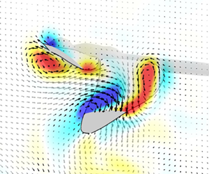
Figure 8 and supplementary movie 2 shows the vortical structures on the wings during when the hindwing downstroke lift peak occurs in escape mode. The iso-surface of Q-criterion shows stronger LEV on the hindwing in escape mode, which could account for the lift enhancement. Note that the non-dimensional time at t/T = 0.12 is defined by the flapping cycle of the hindwing and the apparently different projection of the hindwing view in figure 8 is caused by the difference in pitching kinematics that makes interpretation of the iso-surfaces difficult. For this reason, the Y-vorticity field with velocity vectors at 0.7RHW is also presented in support of the findings. The flow field suggests that the hindwing LEV may be enhanced by interaction with the forewing trailing-edge vortex (TEV) (Hefler et al. Reference Hefler, Qiu and Shyy2018) in escape mode (figure 8 iso-surfaces of Q-criteria). This interaction is affected by the distance separating the flapping wings set by the phasing and other kinematic parameters (Hefler et al. Reference Hefler, Qiu and Shyy2018). The forewing downwash also affects the LEV dynamics of the hindwing, as shown by the velocity vector field upstream of the hindwing in figure 8. In escape mode at t/T = 0.12, the hindwing LEV looks expanded chordwise along the upper surface of the wing, suggesting that a downwash may delay the LEV detachment during the downstroke that could also enhance lift. Additionally, the different pitching and flapping kinematics of the hindwing in escape flight naturally affects its LEV.

Figure 8. The Y-vorticity field with velocity vectors at 0.7RHW for normal (case 1) and escape (case 2) flight. Grey, smoke-like object is the iso-surface of Q-criterion at 2.0 × 10⁵ (s−2). The time instant of t/T = 0.12 is the moment when the lift amplification happens on the hindwing.
To quantify the LEV enhancement in escape flight at t/T = 0.12, we can calculate circulation. The LEV circulation was estimated by integration of the vorticity,  $\omega $. The area of integration, $\textrm{d}S$, is bound by the vorticity threshold (25 % of the peak vorticity). The circulation is non-dimensionalized by the product of ${U_{ref}}$ and ${L_{ref}}$:
 \begin{equation}\varGamma _{LEV}^\ast= \frac{1}{{{U_{ref}}{L_{ref}}}}\iint_s {\omega \cdot \textrm{d}S} .\end{equation}
The instantaneous LEV circulation of the hindwing at 0.7RHW in figure 8 is 1.68 in normal flight and 3.21 in escape flight. The dimensional value of the hindwing lift at the peak during downstroke also increases by about the same proportion from 10.9 to 20.8 mN in escape flight.
In normal flight, the forewing generates substantially less thrust (and even drag for a brief period during downstroke) than the hindwing; for the complete cycle, 1.246 versus 2.391 mN (table 2 and figure 6). Thrust is generated by the forewing most prominently during upstroke, agreeing with the previous findings regarding hovering dragonfly flight with inclined strokes and asymmetric pitching (Sun & Lan Reference Sun and Lan2004; Wang & Sun Reference Wang and Sun2005; Wang & Russell Reference Wang and Russell2007; Hu & Deng Reference Hu and Deng2014; Liu et al. Reference Liu, Hefler, Fu, Shyy and Qiu2021a). Interestingly the hindwing is able to generate thrust during the downstroke in the normal flight mode and during the first half of the downstroke in the escape mode, which accounts for some of the difference in thrust performance between the wings. It is likely that the thrust and lift forces of the hindwing are distributed differently from those of the forewing due to the difference in local angle of attack (see the pitching and twisting of the wings in figure 4), helping the hindwing to generate thrust during the downstroke but at the expense of lift. This could also explain that during most of the downstroke in normal flight, the lift of the hindwing is almost equal to that of the forewing although the added mass effect of the larger wing surface would warrant it being higher (Sun & Lan Reference Sun and Lan2004; Liu et al. Reference Liu, Hefler, Fu, Shyy and Qiu2021a).
3.3 The role of wing phasing (cases 1 and 3)
The complex interrelations between the kinematic parameters and the resulting aerodynamic features of the normal and escape flight modes are further investigated by changing selected kinematic parameters only in comparison with the reference normal flight mode. First, the role of the wing phasing is studied. In case 3, only the wing phasing is set to the escape flight phasing. Figure 9 presents the vector diagram of the cycle-averaged total force as well as the force by each wing in normal flight (red arrows) and in case 3 (black and purple arrows).

Figure 9. Vector diagram of (a) the cycle-averaged total force as well as (b,c) the force by each wing in case 1 (red arrows) and in case 3 (black and purple arrows).
With only the wings flapping more in phase in this parametric case, the total cycle-averaged thrust coefficient considering both wings increased by 0.017 and the total lift coefficient decreased by 0.011 (table 2), that is, less than the change between the reference normal and escape case discussed above (we confirmed this using the original dimensional values that are available in Appendix E; table 8). Consequently, the total force is slightly increased and slightly more horizontally directed (figure 9). It should be noted that the phasing change we observed when dragonflies switch to escape flight (Liu et al. Reference Liu, Hefler, Shyy and Qiu2021b), as well as the change particularly adopted for the current investigations, is only 36° that is rather small considering the physiological capabilities of dragonflies. Some possible flight scenarios may involve larger phase changes than what was measured in the case of escape mode (Alexander Reference Alexander1984; Wang & Russell Reference Wang and Russell2007). Figure 10 shows the time history of force coefficients for case 3. Compared with the reference case of normal flight (case 1; figure 6), we can see only a slight change in force peak values and time histories, confirming that in the present set-up, the phasing only has a marginal effect on the aerodynamics of the dragonfly. This does not necessarily mean that the interaction between the fore- and hindwings is not important, only that the interaction does not change much. Wing–wing interactions in dragonfly flight most apparently affect the LEV of the hindwing. Figure 11 shows the instantaneous LEV circulation of the hindwing at mid-span (0.5RHW) in case 1 and case 3 for reference. The LEV circulation of the hindwing also confirms that the phasing change has only a marginal effect.

Figure 10. Case 3 – aerodynamic force coefficients over a complete flapping cycle. Kinematics of reference case 1 with the phasing of escape flight. The flapping positional angle (Fourier approximation), as defined in the numerical model with the origin set in each wing's own root fixed coordinate system, is drawn and colour shaded for easier interpretation of the flapping cycle.

Figure 11. Circulation of the LEV of the hindwing at mid-span (0.5RHW) in case 1 and case 3 during the downstroke.
3.4 The role of stroke plane tilting and changing wing pitching (cases 1 and 4)
To study the effect of the local angle of attack, in the parametric model of case 4, the stroke plane and the pitching of the wings in the reference model of normal flight were adjusted to their escape flight values (table 1). Considering the added effect of the change of stroke plane angle and the mean of the pitching angles, the resultant forces of the fore- and hindwings are expected to be tilted upward proportional to the change of the mean kinematic angles that are 13.2° for the forewing and 21° for the hindwing. Figure 12 presents the vector diagram of the cycle-averaged total force as well as the force by each wing in case 1 (red arrows) and in case 4 (black and purple arrows) featuring the angle of the resultant forces for reference. The direction of the resultant force of the forewing changes by 22° and that of the hindwing changes by 39°, which is about 1.66 times and 1.86 times the change of the mean kinematic angles of the fore- and hindwing respectively. The difference between the change in the mean kinematic angles and the change in the direction of the resultant forces is large and it indicates that not only the direction of the resultant force changed but the unsteady aerodynamics (LEV most prominently) of force generation were also affected by the change of the local angle of attack. The total cycle-averaged force of the dragonfly was also directed 32° more vertically, which is about twice the change found in the case of the normal reference flight to the escape flight switch.

Figure 12. Vector diagram of (a) the cycle-averaged total force as well as (b,c) the force by each wing in case 1 (red arrows) and in case 4 (black and purple arrows).
As the angle of attack gets larger during the downstroke and smaller during the upstroke, the total lift coefficient of the complete cycle increases from 0.242 to 0.376 while the thrust decreases from 0.345 to 0.163 (table 2) considering both wings. The lift boost is slightly smaller than the change of the thrust. On the other hand, the total force coefficient of the dragonfly changes only marginally from 0.421 to 0.410 (−3 %), showing that at a systems level, the change of the mean kinematic angles changes the direction of the aerodynamic force but not its magnitude. The power requirement increases and the total efficiency decreases. This explains why such flight has been rarely observed and less studied in the past as it might be feasible only under special temporary circumstances like evasion or hunting.
The cycle-averaged resultant force coefficient of both wings decreases little in the case of the forewing (0.205–0.201) and slightly more in case of the hindwing (0.239–0.215). The lift of the forewing changes little, while the thrust is slightly less than half of the normal mode thrust (table 2 and figure 12). In contrast, for the case of the hindwing, the thrust and lift modulations are about the same. This indicates that the hindwing redistributes about half of the thrust and lift while the forewing only shows a noticeable change in thrust generation.
Figure 13 presents the force coefficient time histories of case 4. Again, referring to figure 6 (case 1) as our reference case, we can confirm that the time histories of the forewing forces are very much alike in normal mode and in this parametric case except for the thrust during the downstroke. During the downstroke, the forewing produces drag that seems to be the sole reason for its thrust modulation. Figure 14 shows the vorticity field and the vector components of the forewing when the thrust modulation occurs (t/T = 0.4) in case 1 and case 4. The force vector diagram is drawn to be centred near the leading edge where the resultant force is perpendicular to the chord and it points towards the centre of the LEV, which plays a significant role in force generation during downstroke. The choice to position the force vector diagram in this way was arbitrary and does not imply that the instantaneous forces at t/T = 0.4 would be the same as the cycle-averaged forces. Figure 14 shows that the increased angle of attack during the downstroke results in a stronger LEV, which explains the slight increase of the lift, while the clockwise pitching of the resultant aerodynamic force redistributes the thrust to the drag.

Figure 13. Case 4 – aerodynamic force coefficients over a complete flapping cycle. Kinematics of reference case 3 with stroke plane and pitching angle of escape flight. The flapping positional angle (Fourier approximation) as defined in the numerical model with the origin set in each wing’s own root fixed coordinate system is drawn and colour shaded for easier interpretation of the flapping cycle.

Figure 14. The Y-vorticity field at 0.6RFW around downstroking forewing in normal fight (case 1) and in parametric case 4, showing the varied wing pitching and its tilting effect on the aerodynamic forces. The arrows represent the lift (dashed line), thrust (solid line) and total force of both forewings at the time instant of t/T = 0.4.
In the case of the hindwing, the force time histories of case 4 and the reference case 1 are again very similar during the upstroke but with less negative lift as the aerodynamic profile of the wing is smaller according to the change of the pitching and the stroke plane. Differently, the hindwing builds up lift earlier in the cycle in case 4 than in case 1 although it generates drag during the entirety of the downstroke. Figure 15 shows the vortex iso-surfaces of Q-criterion as well as the pressure and vorticity at 0.7RHW around the downstroking hindwing in the normal flight (case 1) and in the parametric case 4 at the time instant when the aerodynamic force modulation occurs most noticeably. In figure 15, we can see that the higher angle of attack during the downstroke results in stronger vortex structures around the edges of the hindwing and causes the negative pressure zone above the wing. This increases the lift, while again, the clockwise pitching redistributes the thrust to the drag as seen with the forewing.

Figure 15. The Y-vorticity and pressure fields at 0.7RHW around the downstroking hindwing in normal flight (case 1) and in parametric case 4, showing the varied wing pitching (local angle of attack) and its effect on the formation of the hindwing LEV and TEV. Grey, smoke-like object is the iso-surface of Q-criterion at 5.0 × 10⁵ (s−2). Black lines represent the wing cross-section on each plane. The flow fields under the wings are not visible because they are in the shadow of the wing surface.
Local angle of attack is the most important parameter to affect the formation of the LEV (Ellington et al. Reference Ellington, van den Berg, Willmott and Thomas1996; Thomas et al. Reference Thomas, Taylor, Srygley, Nudds and Bomphrey2004; Shyy & Liu Reference Shyy and Liu2007; Shyy et al. Reference Shyy, Aono, Kang and Liu2013; Wu Reference Wu2018). We also found that, within the confines of our parametric study, the changes in the local angle of attack indeed have a greater effect on dragonfly aerodynamics than the wing phasing.
To complement our observations regarding stroke plane angle and pitch change, we plot the time-averaged velocity iso-surfaces in figure 16. Unlike the change of the wing phasing, the local angle of attack variation results in a noticeable change in the direction of the momentum. Liu et al. (Reference Liu, Hefler, Shyy and Qiu2021b) suggested that besides the effect on LEV formation, the stroke plane angle and pitching adjustments help the dragonfly to direct the momentum, just like the results of our current investigations show.

Figure 16. Absolute velocity iso-surfaces time averaged over a cycle in the wake of the dragonfly in normal flight (case 1) and in parametric case 4. The red surface is 1.75 m s−1; the blue surface is 1.25 m s−1. The red arrows indicate the mean direction of the velocity on the wake and the dashed black lines indicate the body lines.
3.5 Combined effect of phasing and pitching (cases 4 and 5)
Prior investigations show that the phasing of the forewing and hindwing flapping positional angle can vary greatly when dragonflies execute different flight tasks (Wakeling & Ellington Reference Wakeling and Ellington1997; Huang & Sun Reference Huang and Sun2007; Hu & Deng Reference Hu and Deng2014). Interestingly, a more in-phase flapping of the escape flight mode modulates lift and thrust in a way opposite to that of the change of the local angle of attack. To investigate whether phasing may play a more important role in combination with simultaneous adjustments in local angle of attack by pitching and stroke plane angle changes during the flapping cycle, we combine the two previously discussed set-ups in this last parametric case (case 5 in table 2).
Table 2 lists the force and efficiency modulations for case 5. The cycle-averaged total force coefficient and efficiency values do not differ largely from those in case 4. The thrust is slightly increased while the lift is slightly decreased. Although the differences are marginal, the combined effect is advantageous as the thrust coefficient increase is larger (0.021 is the change between case 4 and case 5; 0.017 is the change between case 1 and case 3) and, in addition, the lift coefficient decreases to a smaller extent (0.006 is the change between case 4 and case 5; 0.011 is the change between case 1 and case 3) in comparison with the case when only phasing was considered. Furthermore, the change of power expenditure (CP) in this combined case is less than that of the phase change only (0.01 versus 0.017), and consequently the propulsive efficiency improves slightly as well.
Figure 17 presents the vector diagram of the cycle-averaged total force as well as the force by each wing in case 1 (red arrows) and in case 5 (black and purple arrows) as well as in case 3 (blue arrows) and in case 4 (orange arrows) for an easier interpretation of the phasing effect with/without the change of the mean of the pitching and the stroke plane angle. Figure 17 confirms that the phasing effects on the fore- and hindwing are analogous to the previously discussed case 3.

Figure 17. Vector diagram of (a) the cycle-averaged total force as well as (b,c) the force by each wing in case 1 (red arrows) and in case 5 (black and purple arrows) as well as case 3 (blue arrows) and case 4 (orange arrows).
Figure 18 shows the time histories of the force coefficients over the complete cycle. The time histories of the force coefficients of the wings are almost identical to those seen in case 4, indicating that no additional unsteady interaction mechanism occurs by changing the phase in combination (see also figure 23 in Appendix F). We also see in figure 18 that the curves of the forewing and hindwing are shifted in time according to the phase difference that suppresses the variation in the total lift force during downstroke (the black dashed line in figure 18 has not got the double peaks seen in case 4 or the one large peak seen in the other cases).

Figure 18. Case 5 – aerodynamic force coefficients over a complete flapping cycle. Kinematics of reference case 1 with stroke plane, pitching angle and phasing of escape flight. The flapping positional angle (Fourier approximation), as defined in the numerical model with the origin set in each wing’s own root fixed coordinate system, is drawn and colour shaded for easier interpretation of the flapping cycle.
In case 5, the lift boost of the hindwing during the downstroke as seen in the escape mode (case 2) is not present (figure 18 versus figure 7). Referring to our previous discussion, the results of case 5 also suggest that neither the change in local angle of attack nor the phasing, but more likely the changing of the flapping positional angle (in synergy with the effect of the other kinematics changes) causes the specific flow condition seen in the escape mode (case 2) resulting in the remarkable hindwing lift boost during its downstroke.
4. Conclusions
We numerically studied the role of kinematic manipulation of flapping wings and its interplay with aerodynamics in two distinct flight modes of dragonflies, namely normal forward flight and escape flight. The set kinematic parameters as well as the prescribed wing membrane deformations in this study are based on experimental measurement.
We found that in the escape flight, the cycle-averaged forces of the hindwing are redirected and moderately amplified while the forces of the forewing are reduced, resulting in about 15° more upward flight direction and slightly less efficient flight. The aerodynamic efficiency is reduced by about 8 %. We observed qualitative differences in the flow features as well. The change in the local angle of attack affected the development of the wing-bound vortexes and their resultant force. The LEV of the hindwing was affected not only by the change of flapping kinematics but also by the downwash and the shedding vortex of the forewing due to the varied kinematic set-up of the escape flight.
Investigating the effect of the individual kinematic parameters in isolation and in combination provided several further insights. The phasing of the flapping positional angle (the phase by which the hindwing leads the flapping cycle is reduced by 38°) does not affect the aerodynamics substantially by itself; however, in combination with the varied local angle of attack, it suppresses the variation in the total forces and slightly improves the efficiency. The change in the local angle of attack was found to have a major role in force generation and redistribution. The larger angle of attack during the downstroke results in lift enhancement, while at the same time, the pitching of the wings in the global reference frame tilts the resultant forces that explain the reduced thrust in the escape mode. Finally, in escape flight, the hindwing receives a large lift boost during the downstroke, which was not observed in the studied parametric cases, suggesting that, in addition to the investigated parameters, the adjustments of the flapping positional angle are necessary to obtain a lift boost.
It should be noted that wing kinematics, wing deformations and aerodynamics are strongly coupled in dragonflies, and the unified prescribed deformation of the wing may lead to results different from those of actual flight. However, the presented results based on the observed aerodynamic characteristics may help in designing kinematic controls and actuation mechanisms for micro air vehicles. The insight gained in this study can help advance flight design for microscale air vehicles.
Supplementary movies
Supplementary movies are available at https://doi.org/10.1017/jfm.2023.471.
Acknowledgements
The authors would like to express their gratitude to Professor H. Liu from Chiba University for permission to use the computational fluid dynamics code.
Funding
This work was supported by the Research Grants Council of the Government of Hong Kong Special Administrative Region (HKSAR) with RGC/GRF project no. 16206321 and was partly supported by JSPS KAKENHI grant nos. JP20H05752 and JP23K03733.
Declaration of interests
The authors report no conflict of interest.
Data availability
The data that support the findings of this study are available from the corresponding author upon reasonable request.
Appendix A. Comparison of flow field between experimental and numerical results
Besides the parametric study cases, we simulated two actual flights of the same dragonfly (one normal flight and one escape flight) so we could also directly compare the numerical and experimental results of this particular flight. We can observe a reasonable qualitative and quantitative agreement between the cases considering the highly dynamic nature of the flow fields as shown in figure 19.

Figure 19. Vorticity fields around the wings of a dragonfly in a plane close to the wing root. Left column: PIV measurement. Right column: numerical simulation (case 1 and case 2).
Appendix B. General description of the computation conditions
The computation is started from the beginning of the downstroke of the forewings and it is impulsive as can be seen in the spike of aerodynamic forces around t/T = 0 in figure 20. The initial velocities of the flow field are zero. For the convergence of the flow fields, we conducted five cycles of simulation and the results are derived from the final flapping cycle of the hindwing. The cycle-averaged values during these five cycles are shown in table 3 and the percentage represents the comparison between the current cycle and the previous cycle's values.

Figure 20. Time courses of the horizontal and vertical forces of case 1.
Table 3. Cycle-averaged horizontal and vertical forces of case 1.

Appendix C. Sensitivity study for numerical model
Sensitivity analyses on time step and domain size were performed through the normal (case 1) and escape (case 2) flight modes. Although there is some difference between the cycle-averaged horizontal/vertical forces of the basic and the other models (tables 4 and 5), we consider that the effects on the discussed flow features in this study are minor as can be seen in the time courses of the aerodynamic forces (figure 21).
Table 4. Parameters for sensitivity study and cycle-averaged forces of case 1.

Table 5. Parameters for sensitivity study and cycle-averaged forces of case 2.


Figure 21. Horizontal and vertical forces of (a) case1 (normal flight mode) and (b) case2 (escape flight mode) over a cycle for sensitivity analysis on time step and domain size. Note that these horizontal/vertical forces are the sum of the aerodynamic forces acting on two forewings and two hindwings in each case.
Appendix D. Sensitivity study for the grid spacing resolution
The local wing grids of the basic model have 18 meshes in the chord direction and the boundary conditions at the outermost of the local wing and body grids are given (interpolated) by the global grid. Because of this, the size of the uniform grid is set to be almost the same size as the outermost grid size of the wings. We conducted a sensitivity study as shown in figure 22 and tables 6 and 7. Note that the domain size and time step are the same as those of the basic model in tables 4 and 5. In addition, the two fore- and hindwing grids are the same number in this computation.

Figure 22. Horizontal and vertical force coefficients of (a) the forewings and (b) the hindwings over a cycle for sensitivity analysis on the mesh size. Note that these horizontal/vertical force coefficients are the sum of the aerodynamic forces acting on two forewings and two hindwings in case1.
Table 6. Parameters for sensitivity study and cycle-averaged forces of case 1.

Table 7. Parameters for sensitive study and cycle-averaged forces of case 2.

Although there is some difference between the cycle-averaged vertical force of the finer and the basic grid systems, the effect on the discussed flow features and on the aerodynamic forces is minor. Thus the basic grid system was adopted for this study since the fine grid system would be computationally more expensive.
Appendix E. Dimensional values of forces, power and efficiencies
Thrust and lift forces of the wing pairs, aerodynamic power and efficiency are shown in table 8.
Table 8. Thrust and lift forces of the wing pairs, aerodynamic power and efficiency. The difference between each case and the reference case (case 1) is expressed in percentage.

Appendix F. Comparison of the force time histories in case 4 and case 5
To evaluate whether phasing in combination with simultaneous adjustments in local angle of attack by pitching and stroke plane angle changes during the flapping cycle would trigger additional unsteady interaction effects, we can compare the force time histories in case 4 and case 5.

Figure 23. Aerodynamic force coefficients over a complete flapping cycle in case 4 and case 5 (the forces of the forewing in case 5 are shifted in time to aid comparison). Here t/T = 0 indicates the time when the hindwing starts its downstroke.


 Open access