


1 Introduction
Estimating moments of families of L-functions is a central problem in analytic number theory not only due to their substantial applications, but also since they give an insight into the behaviour of L-functions in the critical strip. Our interests lie in the $2k$
th moments of the Riemann zeta and Dirichlet L-functions:
$2k$
th moments of the Riemann zeta and Dirichlet L-functions:
 $$ \begin{align*} \mathcal{Z}_{k}(g) = \int_{-\infty}^{\infty} \left|\zeta \left(\frac{1}{2}+it \right) \right|^{2k} g(t) dt, \qquad \mathcal{Z}_{k}(g; \chi) = \int_{-\infty}^{\infty} \left|L \left(\frac{1}{2}+it, \chi \right) \right|^{2k} g(t) dt, \end{align*} $$
where $k \geqslant 1$
is an integer and the test function g is of rapid decay. The initial cases
$k \geqslant 1$
is an integer and the test function g is of rapid decay. The initial cases $k = 1, 2$
have been successfully studied for
$k = 1, 2$
have been successfully studied for $\mathcal {Z}_{k}(g)$
, and the other cases have remained untouched thus far. In this article, we establish Motohashi’s formula (also known as a spectral reciprocity formula) for the fourth moment of Dirichlet L-functions, which was unsolved since being posed as a question of study by Motohashi in 1992.
$\mathcal {Z}_{k}(g)$
, and the other cases have remained untouched thus far. In this article, we establish Motohashi’s formula (also known as a spectral reciprocity formula) for the fourth moment of Dirichlet L-functions, which was unsolved since being posed as a question of study by Motohashi in 1992.
1.1 Overview and motivation
In the 1990s, Motohashi [Reference Motohashi55, Theorem 4.2] pondered a mysterious identity relating the smoothed fourth moment of the Riemann zeta function $\zeta (1/2+it)$
to a spectral cubic moment of automorphic L-functions associated to the group
$\zeta (1/2+it)$
to a spectral cubic moment of automorphic L-functions associated to the group $\operatorname {\mathrm {SL}}_{2}(\mathbb {Z})$
. We assume a fixed test function g to be of Schwartz class, and we denote by
$\operatorname {\mathrm {SL}}_{2}(\mathbb {Z})$
. We assume a fixed test function g to be of Schwartz class, and we denote by $\mathcal {B}(q, \chi )$
the set of Hecke–Maaß forms of level q and central character
$\mathcal {B}(q, \chi )$
the set of Hecke–Maaß forms of level q and central character $\chi $
; we write
$\chi $
; we write $\mathcal {B}(\Gamma _{0}(q))$
as usual when
$\mathcal {B}(\Gamma _{0}(q))$
as usual when $\chi $
is principal. His formula then asserts that the following spectral decomposition holds up to an explicit description of holomorphic, Eisenstein and residual contributions that we shall elide here:
$\chi $
is principal. His formula then asserts that the following spectral decomposition holds up to an explicit description of holomorphic, Eisenstein and residual contributions that we shall elide here:
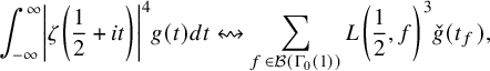 $$ \begin{align} \int_{-\infty}^{\infty} \left|\zeta \left(\frac{1}{2}+it \right) \right|^{4} g(t) dt \leftrightsquigarrow \sum_{f \in \mathcal{B}(\Gamma_{0}(1))} L \left(\frac{1}{2}, f \right)^{3} \check{g}(t_{f}), \end{align} $$
where $\check {g}$
is an elaborate integral transform of g involving the Gauß hypergeometric function. The right-hand side of equation (1.1) must be understood as a complete integral over the full spectrum of level 1 automorphic forms, including holomorphic, discrete and continuous spectra. Motohashi has given several approaches in the spirit of analytic number theory and representation theory. Note that all of his methods are in the framework of relative trace formulæ. On the other hand, Michel–Venkatesh ([Reference Michel and Venkatesh49, §4.3.3], [Reference Michel and Venkatesh50, §4.5.3]) suggested an elegant geometric and spectral stratagem to substantiate equation (1.1). Following their perspective, Nelson [Reference Nelson58] studied the cubic moment of automorphic L-functions on
$\check {g}$
is an elaborate integral transform of g involving the Gauß hypergeometric function. The right-hand side of equation (1.1) must be understood as a complete integral over the full spectrum of level 1 automorphic forms, including holomorphic, discrete and continuous spectra. Motohashi has given several approaches in the spirit of analytic number theory and representation theory. Note that all of his methods are in the framework of relative trace formulæ. On the other hand, Michel–Venkatesh ([Reference Michel and Venkatesh49, §4.3.3], [Reference Michel and Venkatesh50, §4.5.3]) suggested an elegant geometric and spectral stratagem to substantiate equation (1.1). Following their perspective, Nelson [Reference Nelson58] studied the cubic moment of automorphic L-functions on $\operatorname {\mathrm {PGL}}_{2}$
via the use of the regularised diagonal periods of products of Eisenstein series. We also refer the reader to work of Wu et al. [Reference Balkanova, Frolenkov and Wu4, Reference Wu68].
$\operatorname {\mathrm {PGL}}_{2}$
via the use of the regularised diagonal periods of products of Eisenstein series. We also refer the reader to work of Wu et al. [Reference Balkanova, Frolenkov and Wu4, Reference Wu68].
In terms of automorphic representation theoretic language, the spectral reciprocity formula in equation (1.1) is a connection between the fourth moment of $\operatorname {\mathrm {GL}}_{1} \ L$
-functions (geometric side) and the cubic moment of
$\operatorname {\mathrm {GL}}_{1} \ L$
-functions (geometric side) and the cubic moment of $\operatorname {\mathrm {GL}}_{2} \ L$
-functions (spectral side). These sides are derived from an application of the relative trace formula. The advancement toward Motohashi’s formula is summarised in the following table.Footnote
1
$\operatorname {\mathrm {GL}}_{2} \ L$
-functions (spectral side). These sides are derived from an application of the relative trace formula. The advancement toward Motohashi’s formula is summarised in the following table.Footnote
1
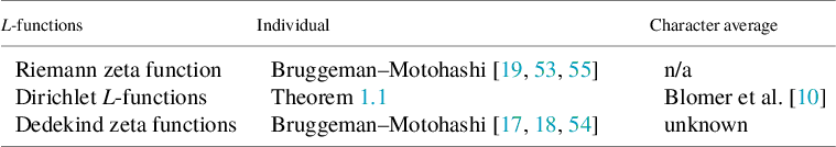
These works share similar structure to Motohashi’s formula in equation (1.1) (compare [Reference Motohashi, Friedberg, Bump, Goldfeld and Hoffstein56]). In particular, the heuristics of Blomer et al. [Reference Blomer, Humphries, Khan and Milinovich10] establishes that the character average of the smoothed fourth moment of Dirichlet L-functions weighted by $\chi (a) \overline {\chi }(b)$
is expressed by means of a cubic moment of L-functions associated to Hecke–Maaß newforms of level
$\chi (a) \overline {\chi }(b)$
is expressed by means of a cubic moment of L-functions associated to Hecke–Maaß newforms of level $ab$
. Their method relies on brute force calculations and is cleverer than in [Reference Motohashi55] in the sense that their reasoning is rather symmetric and utilises additive reciprocity. There exist several articles in the antecedent literature on such a fourth moment problem; see [Reference Heath-Brown30, Reference Jutia and Motohashi41, Reference Young69]. Although these achievements address the problem of obtaining an asymptotic, one must go through a harder route to prove Motohashi’s formula.
$ab$
. Their method relies on brute force calculations and is cleverer than in [Reference Motohashi55] in the sense that their reasoning is rather symmetric and utilises additive reciprocity. There exist several articles in the antecedent literature on such a fourth moment problem; see [Reference Heath-Brown30, Reference Jutia and Motohashi41, Reference Young69]. Although these achievements address the problem of obtaining an asymptotic, one must go through a harder route to prove Motohashi’s formula.
There are two versions of spectral reciprocity formulæ: $\operatorname {\mathrm {GL}}_{4} \times \operatorname {\mathrm {GL}}_{2} \leftrightsquigarrow \operatorname {\mathrm {GL}}_{4} \times \operatorname {\mathrm {GL}}_{2}$
and
$\operatorname {\mathrm {GL}}_{4} \times \operatorname {\mathrm {GL}}_{2} \leftrightsquigarrow \operatorname {\mathrm {GL}}_{4} \times \operatorname {\mathrm {GL}}_{2}$
and $\operatorname {\mathrm {GL}}_{2} \times \operatorname {\mathrm {GL}}_{2} \leftrightsquigarrow \operatorname {\mathrm {GL}}_{3} \times \operatorname {\mathrm {GL}}_{2}$
. The former instance involves work of Andersen–Kıral [Reference Andersen and Kıral1], Blomer–Khan [Reference Blomer and Khan11, Reference Blomer and Khan12], Blomer–Li–Miller [Reference Blomer, Li and Miller13], Humphries–Khan [Reference Humphries and Khan33], Jana–Nunes [Reference Jana and Nunes40], Kuznetsov [Reference Kuznetsov and Askey47], Nunes [Reference Nunes59] and Zacharias [Reference Zacharias71]. The latter involves work of Blomer et al. [Reference Blomer, Humphries, Khan and Milinovich10], Nelson [Reference Nelson58], Petrow [Reference Petrow62], Petrow–Young [Reference Petrow and Young63, Reference Petrow and Young64], Wu [Reference Wu68] and Young [Reference Young69]. It behooves one to touch on the article in preparation due to Humphries–Khan to deduce
$\operatorname {\mathrm {GL}}_{2} \times \operatorname {\mathrm {GL}}_{2} \leftrightsquigarrow \operatorname {\mathrm {GL}}_{3} \times \operatorname {\mathrm {GL}}_{2}$
. The former instance involves work of Andersen–Kıral [Reference Andersen and Kıral1], Blomer–Khan [Reference Blomer and Khan11, Reference Blomer and Khan12], Blomer–Li–Miller [Reference Blomer, Li and Miller13], Humphries–Khan [Reference Humphries and Khan33], Jana–Nunes [Reference Jana and Nunes40], Kuznetsov [Reference Kuznetsov and Askey47], Nunes [Reference Nunes59] and Zacharias [Reference Zacharias71]. The latter involves work of Blomer et al. [Reference Blomer, Humphries, Khan and Milinovich10], Nelson [Reference Nelson58], Petrow [Reference Petrow62], Petrow–Young [Reference Petrow and Young63, Reference Petrow and Young64], Wu [Reference Wu68] and Young [Reference Young69]. It behooves one to touch on the article in preparation due to Humphries–Khan to deduce $\operatorname {\mathrm {GL}}_{3} \times \operatorname {\mathrm {GL}}_{2} \leftrightsquigarrow \operatorname {\mathrm {GL}}_{4} \times \operatorname {\mathrm {GL}}_{1}$
reciprocity. This renders an extension of Motohashi’s formula in equation (1.1).
$\operatorname {\mathrm {GL}}_{3} \times \operatorname {\mathrm {GL}}_{2} \leftrightsquigarrow \operatorname {\mathrm {GL}}_{4} \times \operatorname {\mathrm {GL}}_{1}$
reciprocity. This renders an extension of Motohashi’s formula in equation (1.1).
1.2 Statement of main result
Let $\chi $
be an arbitrary primitive Dirichlet character modulo an integer q, and let
$\chi $
be an arbitrary primitive Dirichlet character modulo an integer q, and let $\mathcal {R}_{4}^{+}$
be a subdomain of
$\mathcal {R}_{4}^{+}$
be a subdomain of $\mathbb {C}^{4}$
, where all four parameters have real parts greater than one. In this article, we update the progress toward spectral reciprocity formulæ and extend equation (1.1) to the fourth moment of individual Dirichlet L-functions associated to
$\mathbb {C}^{4}$
, where all four parameters have real parts greater than one. In this article, we update the progress toward spectral reciprocity formulæ and extend equation (1.1) to the fourth moment of individual Dirichlet L-functions associated to $\chi $
in the t-aspect. Thus the setup that we build upon is as follows. For
$\chi $
in the t-aspect. Thus the setup that we build upon is as follows. For $q \in \mathbb {N}$
, we consider
$q \in \mathbb {N}$
, we consider
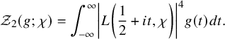 $$ \begin{align} \mathcal{Z}_{2}(g; \chi) = \int_{-\infty}^{\infty} \left|L \left(\frac{1}{2}+it, \chi \right) \right|^{4} g(t) dt. \end{align} $$
This is seen as a character analogue of equation (1.1). The twist by $\chi $
substantially complicates our analysis, and we will encounter various intricate character sums. If g is a sufficiently nice test function, then we define
$\chi $
substantially complicates our analysis, and we will encounter various intricate character sums. If g is a sufficiently nice test function, then we define
 $$ \begin{align} \mathcal{Z}_{2}(s_{1}, s_{2}, s_{3}, s_{4}; g; \chi) = \int_{-\infty}^{\infty} L(s_{1}+it, \chi) L(s_{2}+it, \chi) L(s_{3}-it, \overline{\chi}) L(s_{4}-it, \overline{\chi}) g(t) dt, \end{align} $$
where the parameters or shifts satisfy $(s_{1}, s_{2}, s_{3}, s_{4}) \in \mathcal {R}_{4}^{+}$
. In order to establish Motohashi’s formula for the fourth moment in equation (1.2), we initially work with equation (1.3) by exploiting Dirichlet series expansions for the integrand in the region of absolute convergence, and we take the limit
$(s_{1}, s_{2}, s_{3}, s_{4}) \in \mathcal {R}_{4}^{+}$
. In order to establish Motohashi’s formula for the fourth moment in equation (1.2), we initially work with equation (1.3) by exploiting Dirichlet series expansions for the integrand in the region of absolute convergence, and we take the limit $(s_{1}, s_{2}, s_{3}, s_{4}) \to (1/2, 1/2, 1/2, 1/2)$
after the meromorphic continuation as in the original work of Motohashi [Reference Motohashi55].
$(s_{1}, s_{2}, s_{3}, s_{4}) \to (1/2, 1/2, 1/2, 1/2)$
after the meromorphic continuation as in the original work of Motohashi [Reference Motohashi55].
We proceed to the rigorous statement of our reciprocity formula, which requires a bit of notation. For simplicity, we assume that q is prime. The classification of automorphic forms is convenient in the sequel:
-
• Cuspidal holomorphic newforms f of weight $k \equiv \kappa (\psi ) = \kappa \pmod {2}$
, level q, central character
$\psi $
and Hecke eigenvalues
$\lambda _{f}(n) \in \mathbb {C}$
; we denote the set of such forms by
$\mathcal {B}_{k}^{\ast }(q, \psi )$
;
$k \equiv \kappa (\psi ) = \kappa \pmod {2}$
, level q, central character
$\psi $
and Hecke eigenvalues
$\lambda _{f}(n) \in \mathbb {C}$
; we denote the set of such forms by
$\mathcal {B}_{k}^{\ast }(q, \psi )$
; -
• Cuspidal Maaß newforms f of spectral parameter
$t_{f} \in \mathbb {R} \cup [-i\vartheta , i\vartheta ]$
, weight
$\kappa = (1-\psi (-1))/2$
, level q, central character
$\psi $
and Hecke eigenvalues
$\lambda _{f}(n) \in \mathbb {C}$
, where at the current state of knowledge,
$\vartheta = 7/64$
can be taken (see [Reference Kim45]; although
$\vartheta = 0$
is expected); we denote the set of such forms by
$\mathcal {B}_{\kappa }^{\ast }(q, \psi )$
; -
• Unitary Eisenstein series
$E(z, s, f)$
, where
$s = 1/2+it$
with
$t \in \mathbb {R} \setminus \{0 \}$
and
$\mathcal {B}(\psi _{1}, \psi _{2}) \ni f$
with
$\psi = \psi _{1} \psi _{2}$
is a certain finite set depending upon
$\psi _{1}, \psi _{2}$
corresponding to an orthonormal basis in the space of the induced representation constructed out of
$(\psi _{1}, \psi _{2})$
. Their nth Hecke eigenvalue is written as
$\lambda _{f}(n, t) = \sum _{ab = n} \psi _{1}(a) a^{it} \psi _{2}(b) b^{-it}$
for
$(n, q) = 1$
.


Let $\tau (\chi )$
and
$\tau (\chi )$
and $J(\chi , \psi )$
be the Gauß sum and the Jacobi sum, respectively, so that we define
$J(\chi , \psi )$
be the Gauß sum and the Jacobi sum, respectively, so that we define $\mathcal {H}_{\pm }(\chi , \psi ) = \psi (\mp 1) \tau (\psi ) \tau (\overline {\chi \psi }) J(\psi , \psi )$
. For a test function as in Convention 1.10, we define the spectral mean valuesFootnote
2
$\mathcal {H}_{\pm }(\chi , \psi ) = \psi (\mp 1) \tau (\psi ) \tau (\overline {\chi \psi }) J(\psi , \psi )$
. For a test function as in Convention 1.10, we define the spectral mean valuesFootnote
2

where
and $\mathcal {J}_{\pm }^{\;\text {hol}}$
involve the cubic moment of twisted automorphic L-functions and the continuous term
$\mathcal {J}_{\pm }^{\;\text {hol}}$
involve the cubic moment of twisted automorphic L-functions and the continuous term $\mathcal {J}_{\pm }^{\;\text {Eis}}$
should be regarded as the sixth moment of Dirichlet L-functions. Here,
$\mathcal {J}_{\pm }^{\;\text {Eis}}$
should be regarded as the sixth moment of Dirichlet L-functions. Here, $\#$
on the sum signifies that the sum runs over all primitive nonquadratic characters modulo q, and we define
$\#$
on the sum signifies that the sum runs over all primitive nonquadratic characters modulo q, and we define
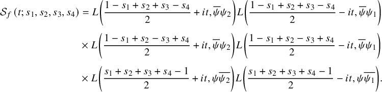 $$ \begin{align} \begin{split} \mathcal{S}_{f}(t; s_{1}, s_{2}, s_{3}, s_{4}) & = L \left(\frac{1-s_{1}+s_{2}+s_{3}-s_{4}}{2}+it, \overline{\psi} \psi_{2} \right) L \left(\frac{1-s_{1}+s_{2}+s_{3}-s_{4}}{2}-it, \overline{\psi} \psi_{1} \right)\\[3pt] & \times L \left(\frac{1-s_{1}+s_{2}-s_{3}+s_{4}}{2}+it, \overline{\psi} \psi_{2} \right) L \left(\frac{1-s_{1}+s_{2}-s_{3}+s_{4}}{2}-it, \overline{\psi} \psi_{1} \right)\\[3pt] & \times L \left(\frac{s_{1}+s_{2}+s_{3}+s_{4}-1}{2}+it, \psi \overline{\psi_{2}} \right) L \left(\frac{s_{1}+s_{2}+s_{3}+s_{4}-1}{2}-it, \psi \overline{\psi_{1}} \right). \end{split} \end{align} $$
The factor $\epsilon _{f}$
in the summand denotes the parity of a Maaß form f. In addition,
$\epsilon _{f}$
in the summand denotes the parity of a Maaß form f. In addition, $\Phi _{\texttt {s}}^{\pm }$
and
$\Phi _{\texttt {s}}^{\pm }$
and $\Xi _{\texttt {s}}$
are introduced in equations (3.26), (3.27) and (3.28), respectively. The Dirichlet series expansions of the adjoint square L-function
$\Xi _{\texttt {s}}$
are introduced in equations (3.26), (3.27) and (3.28), respectively. The Dirichlet series expansions of the adjoint square L-function $L(s, \mathrm {Ad}^{2} f)$
, and the twisted automorphic L-function
$L(s, \mathrm {Ad}^{2} f)$
, and the twisted automorphic L-function $L(s, f \otimes \psi )$
in
$L(s, f \otimes \psi )$
in $\Re (s)> 1$
(that serve as a definition of these functions) are given in equations (2.24) and (2.25), respectively. We are now ready to describe the reciprocity formula to which we have alluded previously.
$\Re (s)> 1$
(that serve as a definition of these functions) are given in equations (2.24) and (2.25), respectively. We are now ready to describe the reciprocity formula to which we have alluded previously.
Theorem 1.1. Let $\chi $
be a primitive Dirichlet character modulo a prime q, and let
$\chi $
be a primitive Dirichlet character modulo a prime q, and let $\texttt {s} = (s_{1}, s_{2}, s_{3}, s_{4})$
with
$\texttt {s} = (s_{1}, s_{2}, s_{3}, s_{4})$
with $\overline {\texttt {s}} = (\overline {s_{3}}, \overline {s_{4}}, \overline {s_{2}}, \overline {s_{1}})$
. Let
$\overline {\texttt {s}} = (\overline {s_{3}}, \overline {s_{4}}, \overline {s_{2}}, \overline {s_{1}})$
. Let $(s_{1}, s_{2}, s_{3}, s_{4}) \in \mathbb {C}^{4}$
be such that
$(s_{1}, s_{2}, s_{3}, s_{4}) \in \mathbb {C}^{4}$
be such that $|s_{1}|, |s_{2}|, |s_{3}|, |s_{4}| < B$
with B sufficiently large. If a test function g satisfies the basic assumption in Convention 1.10, then we have that
$|s_{1}|, |s_{2}|, |s_{3}|, |s_{4}| < B$
with B sufficiently large. If a test function g satisfies the basic assumption in Convention 1.10, then we have that
 $$ \begin{align} \mathcal{Z}_{2}(\texttt{s}; g; \chi) = \mathcal{N}(\texttt{s}; g; \chi) + \sum_{\pm} \left(\mathcal{J}_{\pm}(\texttt{s}; g; \chi)+\mathcal{E}_{\pm}(\texttt{s}; g; \chi) + \overline{\mathcal{J}_{\pm}(\overline{\texttt{s}}; g; \chi)}+\overline{\mathcal{E}_{\pm}(\overline{\texttt{s}}; g; \chi)} \right), \end{align} $$
where $\mathcal {N}$
is an explicitly computable main term, and we decompose
$\mathcal {N}$
is an explicitly computable main term, and we decompose

Here $ \mathcal {E}_{\pm }(\texttt {s}; g; \chi )$
is the degenerate term defined in Section 3.5.2, which has similar shape to
$ \mathcal {E}_{\pm }(\texttt {s}; g; \chi )$
is the degenerate term defined in Section 3.5.2, which has similar shape to $\mathcal {J}_{\pm }(\texttt {s}; g; \chi )$
.
$\mathcal {J}_{\pm }(\texttt {s}; g; \chi )$
.
It should be feasible to generalise Theorem 1.1 to the case of any positive integer q. If q is not prime, we need to utilise a general version of the transformation formula due to Blomer–Milićević [Reference Blomer and Milićević15, (2.2)]:
 $$ \begin{align} \sum_{(c, q) = 1} \chi(c) S(m, n; c) h(c) = \frac{\chi_{1}(m)}{\tau(\chi_{1})} \sum_{d \mid q} \mu(d) \sum_{dq_{1} \mid c} S_{\chi_{1}}(m, nq_{1}^{2}; c) h \left(\frac{c}{q_{1}} \right). \end{align} $$
This is valid for an arbitrary Dirichlet character modulo q induced from a primitive character $\chi _{1}$
modulo
$\chi _{1}$
modulo $q_{1} \mid q$
and for every
$q_{1} \mid q$
and for every $(m, q_{1}) = 1$
. The formula in equation (1.6) translates Kloosterman sums associated to the
$(m, q_{1}) = 1$
. The formula in equation (1.6) translates Kloosterman sums associated to the $(\infty , 0)$
cusp-pair into twisted Kloosterman sums associated to the
$(\infty , 0)$
cusp-pair into twisted Kloosterman sums associated to the $(\infty , \infty )$
cusp-pair. The bottleneck is that the Kloosterman sum on the right-hand side of equation (1.6) involves
$(\infty , \infty )$
cusp-pair. The bottleneck is that the Kloosterman sum on the right-hand side of equation (1.6) involves $q_{1}^{2}$
instead of
$q_{1}^{2}$
instead of $q^{2}$
.
$q^{2}$
.
Remark 1.2. In the author’s recent work [Reference Kaneko44], the second moment of the product of the Riemann zeta and Dirichlet L-functions was contemplated:
 $$ \begin{align} \int_{-\infty}^{\infty} \left|\zeta \left(\frac{1}{2}+it \right) L \left(\frac{1}{2}+it, \chi \right) \right|^{2} g(t) dt. \end{align} $$
If one replaces the Riemann zeta function with a Dirichlet L-function, this is in accordance with equation (1.2). Although the definition in equation (1.2) is similar to equation (1.7), the cubic moment side in Theorem 1.1 has a quite different shape. This is due to the occurrence of additional character sums when we consider the fourth moment of Dirichlet L-functions. However, the resulting form of an integral transform of g never becomes altered.
1.3 Quantitative applications
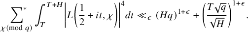
We are able to provide various quantitative applications of Theorem 1.1. A hybrid fourth moment bound of interval H for individual Dirichlet L-functions is initially proven.
Corollary 1.3. Let $T^{1/2} \leqslant H \leqslant T(\log T)^{-1}$
. For any primitive Dirichlet character
$T^{1/2} \leqslant H \leqslant T(\log T)^{-1}$
. For any primitive Dirichlet character $\chi $
modulo a prime q, we have
$\chi $
modulo a prime q, we have
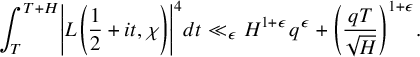 $$ \begin{align} \int_{T}^{T+H} \left|L \left(\frac{1}{2}+it, \chi \right) \right|^{4} dt \ll_{\epsilon} H^{1+\epsilon} q^{\epsilon}+\left(\frac{qT}{\sqrt{H}} \right)^{1+\epsilon}. \end{align} $$
The proof of Corollary 1.3 looks circular at first glance: we use work of Petrow–Young [Reference Petrow and Young63] on cubic moments; they show that bounds for these cubic moments follow from bounds for the fourth moment of Dirichlet L-functions. Nonetheless, this is not circular: Petrow–Young arrive at a long fourth moment that can be bounded optimally via approximate functional equations and the spectral large sieve, whereas our short fourth moment can never be bounded optimally via the spectral large sieve, and it never implies subconvexity. We need to initially apply Motohashi’s formula and then use the large sieve afterward.
Balancing in Corollary 1.3 leads one to a variant of Iwaniec’s [Reference Iwaniec35] short interval fourth moment bound.
Corollary 1.4. Let $q \ll T^{1/2-\epsilon }$
. For any primitive Dirichlet character
$q \ll T^{1/2-\epsilon }$
. For any primitive Dirichlet character $\chi $
modulo a prime q, we have
$\chi $
modulo a prime q, we have
 $$ \begin{align} \int_{T}^{T+(qT)^{2/3}} \left|L \left(\frac{1}{2}+it, \chi \right) \right|^{4} dt \ll_{\epsilon} (qT)^{2/3+\epsilon}. \end{align} $$
Jutila [Reference Jutila42, Theorem 3] obtained the fourth moment bound
 $$ \begin{align} \sum_{\chi\! \pmod{D}} \int_{T}^{T+T^{2/3}} \left|L \left(\frac{1}{2}+it, \chi \right) \right|^{4} dt \ll_{\epsilon} D^{1+\epsilon} T^{2/3+\epsilon}. \end{align} $$
This implies a bound for individual characters of the form $q^{1+\epsilon } T^{2/3+\epsilon }$
. In the range
$q^{1+\epsilon } T^{2/3+\epsilon }$
. In the range $q \ll T^{1/2}$
, our result improves upon this bound for individual characters to
$q \ll T^{1/2}$
, our result improves upon this bound for individual characters to $(qT)^{2/3+\epsilon }$
. There exists a fundamental obstruction that the parameter H in Corollary 1.3 cannot exceed T, and the optimisation of H in the bound in equation (1.8) in turn gives some restriction on q. Indeed, there is a weaker version where one has no restriction on the conductor, which can be deduced from the choice
$(qT)^{2/3+\epsilon }$
. There exists a fundamental obstruction that the parameter H in Corollary 1.3 cannot exceed T, and the optimisation of H in the bound in equation (1.8) in turn gives some restriction on q. Indeed, there is a weaker version where one has no restriction on the conductor, which can be deduced from the choice $H = T^{2/3}$
in Corollary 1.3. It therefore follows that
$H = T^{2/3}$
in Corollary 1.3. It therefore follows that
 $$ \begin{align*} \int_{T}^{T+T^{2/3}} \left|L \left(\frac{1}{2}+it, \chi \right) \right|^{4} dt \ll_{\epsilon} q^{1+\epsilon} T^{2/3+\epsilon}. \end{align*} $$
This is similar to equation (1.10) but eventually yields weaker subconvexity bounds for Dirichlet L-functions.
Corollary 1.4 is equivalent to the claim that Dirichlet L-functions cannot sustain large values, namely
 $$ \begin{align*} \# \left\{t \in \left[T, T+(qT)^{2/3} \right]: \left|L \left(\frac{1}{2}+it, \chi \right) \right| \geqslant V \right\} \ll_{\epsilon} (qT)^{2/3+\epsilon} V^{-4}. \end{align*} $$
It follows that $V \ll (qT)^{1/6+\epsilon }$
, which yields Weyl-strength subconvexity bounds for Dirichlet L-functions when
$V \ll (qT)^{1/6+\epsilon }$
, which yields Weyl-strength subconvexity bounds for Dirichlet L-functions when $q \ll (1+|t|)^{1/2-\epsilon }$
(the exponent
$q \ll (1+|t|)^{1/2-\epsilon }$
(the exponent $1/6$
often reoccurs in modern incarnations of these problems):
$1/6$
often reoccurs in modern incarnations of these problems):
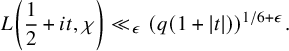 $$ \begin{align*} L \left(\frac{1}{2}+it, \chi \right) \ll_{\epsilon} (q(1+|t|))^{1/6+\epsilon}. \end{align*} $$
This is covered in Petrow–Young [Reference Petrow and Young63, Reference Petrow and Young64], who have shown Weyl-strength subconvexity bounds for twisted automorphic L-functions, which are hybrid in both the t and the q-aspect. We also establish the following:
Corollary 1.5. Assume that $(qT)^{1/2+\epsilon } \ll T_{0} \ll (qT)^{2/3}$
with
$(qT)^{1/2+\epsilon } \ll T_{0} \ll (qT)^{2/3}$
with $q \leqslant T^{1/2-\epsilon }$
and
$q \leqslant T^{1/2-\epsilon }$
and $T \leqslant t_{1} < \cdots < t_{R} \leqslant 2T$
with
$T \leqslant t_{1} < \cdots < t_{R} \leqslant 2T$
with $t_{r+1}-t_{r} \geqslant T_{0}$
. For any primitive Dirichlet character
$t_{r+1}-t_{r} \geqslant T_{0}$
. For any primitive Dirichlet character $\chi $
modulo a prime q, we then have that
$\chi $
modulo a prime q, we then have that
 $$ \begin{align*} \sum_{r = 1}^{R} \int_{t_{r}}^{t_{r}+T_{0}} \left|L \left(\frac{1}{2}+it, \chi \right) \right|^{4} dt \ll_{\epsilon} \left(RT_{0}+qT \sqrt{\frac{R}{T_{0}}} \right)(qT)^{\epsilon}. \end{align*} $$
This kind of fourth moment bound is occasionally seen in the antecedent literature; we mention work of Iwaniec [Reference Iwaniec35] and Jutila–Motohashi [Reference Jutia and Motohashi41] to name two. Since one wants to prove Corollary 1.5 as an application of Theorem 1.1, one exploits the method outlined in the Appendix in Jutila–Motohashi [Reference Jutia and Motohashi41]. They were unable to show Motohashi’s formula for the fourth moment of Dirichlet L-functions averaged over primitive Dirichlet characters, but for the second moment of Estermann zeta functions. The proof of Corollary 1.5 is nearly identical to that of Corollary 1.3; however, one must detect cancellations in the spectral sum, which was executed by Ivić–Motohashi [Reference Ivić and Motohashi34]. We mention that Jutila–Motohashi [Reference Jutia and Motohashi41] established with the same notation as in Corollary 1.5 that
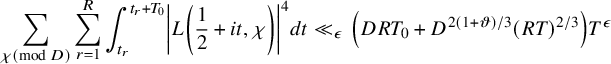 $$ \begin{align*} \sum_{\chi \pmod{D}} \sum_{r = 1}^{R} \int_{t_{r}}^{t_{r}+T_{0}} \left|L \left(\frac{1}{2}+it, \chi \right) \right|^{4} dt \ll_{\epsilon} \left(DRT_{0}+D^{2(1+\vartheta)/3} (RT)^{2/3} \right)T^{\epsilon} \end{align*} $$
with $0 \leqslant \vartheta \leqslant 7/64$
denoting an admissible exponent toward the Ramanujan–Petersson conjecture.
$0 \leqslant \vartheta \leqslant 7/64$
denoting an admissible exponent toward the Ramanujan–Petersson conjecture.
Corollary 1.6. Let $q \ll T^{1/2-\epsilon }$
. For any primitive Dirichlet character
$q \ll T^{1/2-\epsilon }$
. For any primitive Dirichlet character $\chi $
modulo a prime q, we have
$\chi $
modulo a prime q, we have
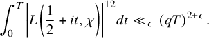 $$ \begin{align} \int_{0}^{T} \left|L \left(\frac{1}{2}+it, \chi \right) \right|^{12} dt \ll_{\epsilon} (qT)^{2+\epsilon}. \end{align} $$
This extends work of Heath-Brown [Reference Heath-Brown29], who obtained the twelfth moment bound
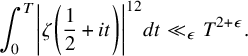 $$ \begin{align} \int_{0}^{T} \left|\zeta \left(\frac{1}{2}+it \right) \right|^{12} dt \ll_{\epsilon} T^{2+\epsilon}. \end{align} $$
One should point out that Heath-Brown deduced equation (1.12) in an entirely different manner via the combination of van der Corput’s method with the Halász–Montgomery inequality. Our method is fundamentally limited in this regard due to the fact that an average over characters is not included; we cannot hope to prove subconvexity bounds for $L(1/2+it, \chi )$
in the q-aspect with t fixed, since we are averaging over too small a family. The result that would be of most interest includes an average over Dirichlet characters modulo q, namely the conjectural upper bound
$L(1/2+it, \chi )$
in the q-aspect with t fixed, since we are averaging over too small a family. The result that would be of most interest includes an average over Dirichlet characters modulo q, namely the conjectural upper bound
 $$ \begin{align*} \sum_{\chi \pmod{q} } \int_{0}^{T} \left|L \left(\frac{1}{2}+it, \chi \right) \right|^{12} dt \ll_{\epsilon} (qT)^{2+\epsilon}. \end{align*} $$
This is a new proof of Weyl-strength subconvexity. If $q = 1$
, this is Heath-Brown’s bound for the twelfth moment of the Riemann zeta function. If
$q = 1$
, this is Heath-Brown’s bound for the twelfth moment of the Riemann zeta function. If $T \ll 1$
and q is a smooth squarefree modulus, this estimate is due to Nunes [Reference Nunes60], although his method does not work for arbitrary q. Meurman [Reference Meurman48] proved the weaker bound
$T \ll 1$
and q is a smooth squarefree modulus, this estimate is due to Nunes [Reference Nunes60], although his method does not work for arbitrary q. Meurman [Reference Meurman48] proved the weaker bound $\mathrm {O}_{\epsilon }(q^{3+\epsilon } T^{2+\epsilon })$
, which implies Weyl-strength subconvexity in the t-aspect but convexity in the q-aspect. Jutila–Motohashi [Reference Jutia and Motohashi41] established that
$\mathrm {O}_{\epsilon }(q^{3+\epsilon } T^{2+\epsilon })$
, which implies Weyl-strength subconvexity in the t-aspect but convexity in the q-aspect. Jutila–Motohashi [Reference Jutia and Motohashi41] established that
 $$ \begin{align*} \sum_{q \leqslant Q} \ \sum_{\chi \pmod{q} } \int_{0}^{T} \left|L \left(\frac{1}{2}+it, \chi \right) \right|^{12} dt \ll_{\epsilon} Q^{3+\epsilon} T^{2+\epsilon}. \end{align*} $$
Milićević–White [Reference Milićević and White51] have studied this problem when $T \ll 1$
and q is growing in the depth aspect.
$T \ll 1$
and q is growing in the depth aspect.
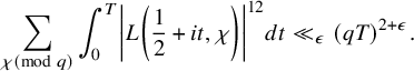
Remark 1.7. It would be interesting to see what happens if we average the fourth moment of individual Dirichlet L-functions over primitive characters modulo q. By brute force, we deduce
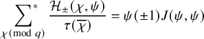 $$ \begin{align*} \sideset{}{^{\ast}} \sum_{\chi \pmod{q} } \frac{\mathcal{H}_{\pm}(\chi, \psi)}{\tau(\overline{\chi})} = \psi(\pm 1) J(\psi, \psi) \end{align*} $$
and this is of absolute value $\sqrt {q}$
, since
$\sqrt {q}$
, since $\psi $
is not quadratic. The final bound looks like
$\psi $
is not quadratic. The final bound looks like
 $$ \begin{align*} \sideset{}{^{\ast}} \sum_{\chi \pmod{q} } \int_{T}^{T+H} \left|L \left(\frac{1}{2}+it, \chi \right) \right|^{4} dt \ll_{\epsilon} (Hq)^{1+\epsilon}+\left(\frac{T \sqrt{q}}{\sqrt{H}} \right)^{1+\epsilon}. \end{align*} $$
Note that this is not completely inconceivable as it does not give any subconvexity bounds, but only the convexity bound due to the presence of the main term. However, there is no hope of getting $(qT)^{2+\epsilon }$
for the twelfth moment, since the bound for the moment in a short interval does not produce subconvexity. In order to circumvent this drawback, the key idea is the following. In the T-aspect, the trick is to divide the integral into shorter intervals and bound each one individually. With an additional sum over Dirichlet characters modulo q, we break this sum into a sum over short cosets. A similar idea is underlying work of Petrow–Young [Reference Petrow and Young63]. We reserve such pursuits for future work.
$(qT)^{2+\epsilon }$
for the twelfth moment, since the bound for the moment in a short interval does not produce subconvexity. In order to circumvent this drawback, the key idea is the following. In the T-aspect, the trick is to divide the integral into shorter intervals and bound each one individually. With an additional sum over Dirichlet characters modulo q, we break this sum into a sum over short cosets. A similar idea is underlying work of Petrow–Young [Reference Petrow and Young63]. We reserve such pursuits for future work.
Finally, Topaçoğullari [Reference Topaçoğullari67] has manifested an asymptotic formula for the fourth moment of individual Dirichlet L-functions. By the specification of a test function g in Theorem 1.1 and a sequence of standard manipulations such as a spectral large sieve, one may arrive at an asymptotic formula of the same quality.
Corollary 1.8 (Topaçoğullari [Reference Topaçoğullari67, Theorem 1.1])
Let $\epsilon> 0$
, which is not necessarily the same at each occurrence. Let
$\epsilon> 0$
, which is not necessarily the same at each occurrence. Let $\chi $
be any primitive Dirichlet character modulo q. Then we have for
$\chi $
be any primitive Dirichlet character modulo q. Then we have for $T \geqslant 1$
that
$T \geqslant 1$
that
 $$ \begin{align} \int_{0}^{T} \left|L \left(\frac{1}{2}+it, \chi \right) \right|^{4} dt = \int_{0}^{T} P_{\chi}(\log t) dt + \mathrm{O}_{\epsilon}(q^{2-3\vartheta} T^{1/2+\vartheta+\epsilon}+qT^{2/3+\epsilon}), \end{align} $$
where $P_{\chi }$
is a polynomial of degree 4 whose coefficients depend only on q.
$P_{\chi }$
is a polynomial of degree 4 whose coefficients depend only on q.
We omit the proof of Corollary 1.8 since our method is quite analogous to that of Topaçoğullari [Reference Topaçoğullari67]. Improving upon the error term in equation (1.13) in the q-aspect requires some additional manoeuvres.
1.4 Sketch of modus operandi
We here render a heuristic overview of the genesis of the automorphic reciprocity shown in Theorem 1.1. This is a high-level sketch geared toward experts. For the sake of argument, we may rely on approximate tools, although our proof is based upon more precise inspection of L-functions in the region of absolute convergence. We must also ignore all correction factors, degenerate terms, polar terms and the t-average.
An astute reader understands our stratagem from the shape of Motohashi’s formula in equation (1.5). The overall ideas are essentially inspired by Motohashi’s seminal work [Reference Motohashi55, §4.3–4.7] that enables one to prove fairly explicit spectral identities. We would like to study what happens if we replace the Riemann zeta function $\zeta (1/2+it)$
in his argument with a Dirichlet L-function
$\zeta (1/2+it)$
in his argument with a Dirichlet L-function $L(1/2+it, \chi )$
, and we observe that the presence of the Dirichlet character substantially complicates our analysis. In a single phrase, we first open the four zeta values as Dirichlet series, apply Atkinson’s dissection and then handle the shifted convolution sums via an application of the Voronoĭ summation formula, followed by the Kloosterman summation formula (Kuznetsov formula) attached to Atkin–Lehner cusps. An initial shape of the off-diagonal term looks like
$L(1/2+it, \chi )$
, and we observe that the presence of the Dirichlet character substantially complicates our analysis. In a single phrase, we first open the four zeta values as Dirichlet series, apply Atkinson’s dissection and then handle the shifted convolution sums via an application of the Voronoĭ summation formula, followed by the Kloosterman summation formula (Kuznetsov formula) attached to Atkin–Lehner cusps. An initial shape of the off-diagonal term looks like
 $$ \begin{align} \sum_{n, m \asymp \sqrt{q}} \overline{\chi}(n) \chi(n+m) \tau(n) \tau(n+m) = \sum_{a, b\! \pmod{q} } \overline{\chi}(a) \chi(a+b) \sum_{\substack{n, m \asymp \sqrt{q} \\ n \equiv a \pmod{q} \\ m \equiv b \pmod{q}}} \tau(n) \tau(n+m). \end{align} $$
This sum has naturally arisen in the antecedent literature such as [Reference Petrow and Young64, Reference Topaçoğullari67, Reference Young69], and $\tau (m)$
must be replaced with the divisor function
$\tau (m)$
must be replaced with the divisor function $\sigma _{\lambda }(m)$
in our proof due to the convergence issue. One sifts out the congruence conditions on the right-hand side of equation (1.14) via primitive additive characters. We can use the orthogonality of the Ramanujan sum
$\sigma _{\lambda }(m)$
in our proof due to the convergence issue. One sifts out the congruence conditions on the right-hand side of equation (1.14) via primitive additive characters. We can use the orthogonality of the Ramanujan sum
 $$ \begin{align*} \delta_{n \equiv a \pmod{q} } = \frac{1}{q} \sum_{c \mid q} r_{c}(n-a). \end{align*} $$
In order to spectrally expand equation (1.14), it is necessary to separate the two variables in $\tau (n+m)$
. We thus make use of the approximate functional equation for the divisor function
$\tau (n+m)$
. We thus make use of the approximate functional equation for the divisor function
 $$ \begin{align} \sigma_{\lambda}(m) = \sum_{(\ell, q) = 1} \frac{S(m, 0; \ell)}{\ell^{1-\lambda}} \varpi_{\lambda} \left(\frac{\ell}{\sqrt{m}} \right) + m^{\lambda} \sum_{(\ell, q) = 1} \frac{S(m, 0; \ell)}{\ell^{1+\lambda}} \varpi_{-\lambda} \left(\frac{\ell}{\sqrt{m}} \right), \end{align} $$
where in the notation of Young [Reference Young69], we set
 $$ \begin{align*} \varpi_{\lambda}(x) = \frac{1}{2\pi i} \int_{(a)} x^{-w} \zeta^{q}(1-\lambda+w) \frac{G(w)}{w} dw. \end{align*} $$
The formula in equation (1.15) is a simple alternative to the $\delta $
-symbol method of Duke–Friedlander–Iwaniec [Reference Duke, Friedlander and Iwaniec22] and plays a rôle in eliminating the pole of the Riemann zeta function
$\delta $
-symbol method of Duke–Friedlander–Iwaniec [Reference Duke, Friedlander and Iwaniec22] and plays a rôle in eliminating the pole of the Riemann zeta function $\zeta (s)$
appearing in the original Ramanujan expansion. In our actual proof, we create a zero that like a deus ex machina kills the pole from the Riemann zeta function. One then applies the
$\zeta (s)$
appearing in the original Ramanujan expansion. In our actual proof, we create a zero that like a deus ex machina kills the pole from the Riemann zeta function. One then applies the $\operatorname {\mathrm {GL}}_{2}$
Voronoĭ summation formula to the sum over n. In other words, the functional equation of the Estermann zeta function is used. Letting
$\operatorname {\mathrm {GL}}_{2}$
Voronoĭ summation formula to the sum over n. In other words, the functional equation of the Estermann zeta function is used. Letting $q \overline {q} \equiv 1 \pmod \ell $
,
$q \overline {q} \equiv 1 \pmod \ell $
, $\ell \overline {\ell } \equiv 1 \pmod q$
and
$\ell \overline {\ell } \equiv 1 \pmod q$
and $\tilde {\tau }(\psi )$
be the normalised Gauß sum, we are led to sums of the product of Kloosterman sumsFootnote
3
$\tilde {\tau }(\psi )$
be the normalised Gauß sum, we are led to sums of the product of Kloosterman sumsFootnote
3
 $$ \begin{align} \sum_{(\ell, q) = 1} \frac{S(m \overline{q}, \pm n \overline{q}; \ell) S(a \overline{\ell}, \pm n \overline{\ell}; q)}{\ell} \approx \sum_{\psi \pmod{q} } \overline{\psi}(\pm anm) \tilde{\tau}(\psi)^{2} \sum_{(\ell, q) = 1} \psi(\ell)^{2} \frac{S(m \overline{q}, \pm n \overline{q}; \ell)}{\ell}. \end{align} $$
Here the second Kloosterman sum $S(a \overline {\ell }, \pm n \overline {\ell }; q)$
was encoded via the orthogonality relation for Dirichlet characters modulo q, and the character
$S(a \overline {\ell }, \pm n \overline {\ell }; q)$
was encoded via the orthogonality relation for Dirichlet characters modulo q, and the character $\overline {\psi }(m)$
was also added on the right-hand side for technical brevity. Be aware of the great similarity between equation (1.16) and Motohashi’s conjecture written down in [Reference Motohashi, Greaves, Harman and Huxley54]. One decomposes the
$\overline {\psi }(m)$
was also added on the right-hand side for technical brevity. Be aware of the great similarity between equation (1.16) and Motohashi’s conjecture written down in [Reference Motohashi, Greaves, Harman and Huxley54]. One decomposes the $\psi $
-sum into the sum over primitive nonquadratic characters and others, followed by the application of the transformation formula due to Blomer–Milićević [Reference Blomer and Milićević15]. We are in a position to use the Kloosterman summation formula of level at most
$\psi $
-sum into the sum over primitive nonquadratic characters and others, followed by the application of the transformation formula due to Blomer–Milićević [Reference Blomer and Milićević15]. We are in a position to use the Kloosterman summation formula of level at most $q^{2}$
and
$q^{2}$
and $(\infty , \infty )$
cusp-pair. In this way, we obtain three automorphic L-functions with an explicit calculation of the resulting sums over m and n, thereby deriving
$(\infty , \infty )$
cusp-pair. In this way, we obtain three automorphic L-functions with an explicit calculation of the resulting sums over m and n, thereby deriving
 $$ \begin{align} &\int_{-\infty}^{\infty} \left|L \left(\frac{1}{2}+it, \chi \right) \right|^{4} g(t) dt \leftrightsquigarrow \sum_{\pm} \sum_{d \mid q} \frac{\mu(d)}{d} \ \sideset{}{^{\#}} \sum_{\psi \pmod{q} } \mathcal{H}_{\pm}(\chi, \psi)\nonumber\\&\qquad\qquad\qquad\qquad\qquad\qquad\qquad \times \sum_{f \in \mathcal{B}_{\kappa}^{\ast}(dq, \psi^{2})} \epsilon_{f}^{(1 \mp 1)/2} \frac{L(1/2, f \otimes \overline{\psi})^{3}}{L(1, \mathrm{Ad}^{2} f)} \check{g}(t_{f}), \end{align} $$
where the character sum $\mathcal {H}_{\pm }(\chi , \psi )$
was defined in Section 1.2 and the transform
$\mathcal {H}_{\pm }(\chi , \psi )$
was defined in Section 1.2 and the transform $\check {g}$
involves the hypergeometric function and depends on
$\check {g}$
involves the hypergeometric function and depends on $\pm $
. The contribution of the quadratic characters is similarly described. A benefit of using Motohashi’s classical method is that one can achieve an explicit formulation of
$\pm $
. The contribution of the quadratic characters is similarly described. A benefit of using Motohashi’s classical method is that one can achieve an explicit formulation of $\check {g}$
, which would be alluring from an aesthetic point of view. If
$\check {g}$
, which would be alluring from an aesthetic point of view. If $\psi $
is a primitive character modulo q and
$\psi $
is a primitive character modulo q and $f \in \mathcal {B}_{\kappa }^{\ast }(dq, \psi ^{2})$
, then
$f \in \mathcal {B}_{\kappa }^{\ast }(dq, \psi ^{2})$
, then $f \otimes \overline {\psi }$
has trivial central character and conductor dividing
$f \otimes \overline {\psi }$
has trivial central character and conductor dividing $q^{2}$
(Theorem A.1). There is some structural beauty in our reciprocity equation (1.17), since we were forced to decompose the
$q^{2}$
(Theorem A.1). There is some structural beauty in our reciprocity equation (1.17), since we were forced to decompose the $\psi $
-sum in terms of whether
$\psi $
-sum in terms of whether $\psi $
is primitive nonquadratic or not. The condition that
$\psi $
is primitive nonquadratic or not. The condition that $f \otimes \overline {\psi }$
has the trivial central character is decisive as we may rely on the result of Guo [Reference Guo27], which guarantees that
$f \otimes \overline {\psi }$
has the trivial central character is decisive as we may rely on the result of Guo [Reference Guo27], which guarantees that $L(1/2, f \otimes \overline {\psi }) \geqslant 0$
. We can then evaluate the cubic moment in equation (1.17) using a standard positivity argument.
$L(1/2, f \otimes \overline {\psi }) \geqslant 0$
. We can then evaluate the cubic moment in equation (1.17) using a standard positivity argument.
There is also a noteworthy plan to contemplate the fourth moment of individual Dirichlet L-functions. Fix a primitive Dirichlet character $\psi $
modulo q. We take
$\psi $
modulo q. We take $b = 1$
in [Reference Blomer, Humphries, Khan and Milinovich10, Theorem 1], multiply
$b = 1$
in [Reference Blomer, Humphries, Khan and Milinovich10, Theorem 1], multiply $\mathcal {T}_{a, b, q}(s, u, v)$
by
$\mathcal {T}_{a, b, q}(s, u, v)$
by $\overline {\psi }(a)$
and then sum over
$\overline {\psi }(a)$
and then sum over $a \pmod q$
with the application of the orthogonality relation. As an aside, this process necessitates a little modification since a is supposed to be squarefree there. Nevertheless, this assumption was only to keep their formulæ cleaner, and hence their method works more generally when a is not squarefree. It is believed that the substantial simplification of [Reference Blomer, Humphries, Khan and Milinovich10, (1.14)] will happen. We remark that the argument in [Reference Blomer, Humphries, Khan and Milinovich10] relies essentially on the isobaric sum
$a \pmod q$
with the application of the orthogonality relation. As an aside, this process necessitates a little modification since a is supposed to be squarefree there. Nevertheless, this assumption was only to keep their formulæ cleaner, and hence their method works more generally when a is not squarefree. It is believed that the substantial simplification of [Reference Blomer, Humphries, Khan and Milinovich10, (1.14)] will happen. We remark that the argument in [Reference Blomer, Humphries, Khan and Milinovich10] relies essentially on the isobaric sum $4 = 3+1$
and dualises
$4 = 3+1$
and dualises $3$
afterward. Its chief novelty is the use of the twisted multiplicativity of Kloosterman sums, enabling us to circumvent the manipulation of Kloosterman sums associated to various Atkin–Lehner cusps.
$3$
afterward. Its chief novelty is the use of the twisted multiplicativity of Kloosterman sums, enabling us to circumvent the manipulation of Kloosterman sums associated to various Atkin–Lehner cusps.
Remark 1.9. This work is relevant to the sixth moment of the Riemann zeta function (see [Reference Kaneko43]) whose calculations were initially contained in this article, but the author decided to remove this part since they are heuristics.
1.5 Organisation of the article
We devote Section 2 to compiling a preparatory toolbox in particular the evaluation of various multiplicative functions followed by the $\operatorname {\mathrm {GL}}_{2}$
Voronoĭ summation formula and the Kloosterman summation formula. We also equip the reader with an exhaustive exposition of Kloosterman sums at various cusps. In Section 3, we prove Theorem 1.1 via a shifted convolution problem. In Section 4, we establish Corollaries 1.3, 1.4, 1.5 and 1.6. The methods involve a combination of classical analytic number theory and automorphic forms. Moreover, the size of the conductor for twists of Maaß newforms is evaluated in Appendix A.
$\operatorname {\mathrm {GL}}_{2}$
Voronoĭ summation formula and the Kloosterman summation formula. We also equip the reader with an exhaustive exposition of Kloosterman sums at various cusps. In Section 3, we prove Theorem 1.1 via a shifted convolution problem. In Section 4, we establish Corollaries 1.3, 1.4, 1.5 and 1.6. The methods involve a combination of classical analytic number theory and automorphic forms. Moreover, the size of the conductor for twists of Maaß newforms is evaluated in Appendix A.
1.6 Basic notation and conventions
Throughout this article, the letter $\epsilon $
represents an arbitrarily small positive quantity, not necessarily the same at each occurrence. An implicit constant may depend on
$\epsilon $
represents an arbitrarily small positive quantity, not necessarily the same at each occurrence. An implicit constant may depend on $\epsilon $
, but this will often be suppressed from the notation. The Vinogradov symbol
$\epsilon $
, but this will often be suppressed from the notation. The Vinogradov symbol $A \ll B$
or the big
$A \ll B$
or the big $\mathrm {O}$
notation
$\mathrm {O}$
notation $A = \mathrm {O}(B)$
signifies that
$A = \mathrm {O}(B)$
signifies that $|A| \leqslant C|B|$
for some constant C. We use the notation
$|A| \leqslant C|B|$
for some constant C. We use the notation
![]() and
and
![]() with
with $\zeta \in \mathbb {C}$
and
$\zeta \in \mathbb {C}$
and $\alpha \in \mathbb {R}$
. We assume that a test function g satisfies the following assumptions:
$\alpha \in \mathbb {R}$
. We assume that a test function g satisfies the following assumptions:
Convention 1.10. The function g is real valued on $\mathbb {R}$
, and there exists a large positive constant A such that
$\mathbb {R}$
, and there exists a large positive constant A such that $g(t)$
is holomorphic and
$g(t)$
is holomorphic and $\ll (1+|t|)^{-A}$
on a sufficiently wide horizontal strip
$\ll (1+|t|)^{-A}$
on a sufficiently wide horizontal strip $|\Im (t)| \leqslant A$
. All implicit constants in Vinogradov symbols and big
$|\Im (t)| \leqslant A$
. All implicit constants in Vinogradov symbols and big $\mathrm {O}$
notation may possibly depend on A (where applicable).
$\mathrm {O}$
notation may possibly depend on A (where applicable).
2 Arithmetic and automorphic tools
We compile background materials that we shall need afterward to establish Theorem 1.1. For starters, we prepare elementary lemmata that are suitable for evaluating the character sums arising in this work. Our focus is on the simplification of sums involving multiplicative characters, which are akin to [Reference Petrow and Young64, §6.1]. Second, we introduce the Estermann zeta function and demonstrate its properties such as a functional equation. Finally, we present automorphic machinery as well as a preliminary exposition of Kloosterman sums. An exhaustive account of the theoretical background is found in [Reference Blomer, Harcos and Michel9, Reference Drappeau21, Reference Duke, Friedlander and Iwaniec23] and references therein.
2.1 Manipulations of character sums
The orthogonality relation asserts that
 $$ \begin{align} \sum_{a\! \pmod q} \chi(a) = \begin{cases} \varphi(q) & \text{if } \chi = \chi_{0},\\ 0 & \text{otherwise}, \end{cases} \qquad \sum_{\chi \pmod{q} } \chi(a) = \begin{cases} \varphi(q) & \text{if } a \equiv 1 \pmod q,\\ 0 & \text{otherwise}. \end{cases} \\[-15pt]\nonumber\end{align} $$
For any Dirichlet character $\chi $
modulo q, let
$\chi $
modulo q, let
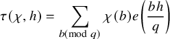 $$ \begin{align} \tau(\chi, h) = \sum_{b\! \pmod q} \chi(b) e \left(\frac{bh}{q} \right) \\[-15pt]\nonumber\end{align} $$
denote the Gauß sum associated to characters on residue classes modulo q. One writes $\tau (\chi ) = \tau (\chi , 1)$
as usual. Multiplying equation (2.2) by
$\tau (\chi ) = \tau (\chi , 1)$
as usual. Multiplying equation (2.2) by $\overline {\chi }(a)$
and summing over
$\overline {\chi }(a)$
and summing over $\chi $
, we derive via orthogonality equation (2.1) that
$\chi $
, we derive via orthogonality equation (2.1) that
 $$ \begin{align} e \left(\frac{ah}{q} \right) = \frac{1}{\varphi(q)} \sum_{\chi \pmod{q} } \overline{\chi}(a) \tau(\chi, h) \quad \text{if} \quad (a, q) = 1.\\[-15pt]\nonumber \end{align} $$
This is the Fourier expansion of additive characters in terms of the multiplicative ones. One can evaluate Gauß sums for general Dirichlet characters.
Lemma 2.1. Let $\chi $
be a nontrivial Dirichlet character modulo q induced by the primitive character
$\chi $
be a nontrivial Dirichlet character modulo q induced by the primitive character $\chi ^{\ast }$
modulo
$\chi ^{\ast }$
modulo $q^{\ast }$
. For an integer
$q^{\ast }$
. For an integer $n \geqslant 1$
, we have that
$n \geqslant 1$
, we have that
 $$ \begin{align*} \tau(\chi, n) = \tau(\chi^{\ast}) \sum_{d \mid (n, q/q^{\ast})} d \overline{\chi^{\ast}} \left(\frac{n}{d} \right) \chi^{\ast} \left(\frac{q}{dq^{\ast}} \right) \mu \left(\frac{q}{dq^{\ast}} \right).\\[-15pt] \end{align*} $$
Proof. See [Reference Iwaniec and Kowalski38, Lemma 3.2], which is corrected in the list of errata on Kowalski’s website.
We indicate by $r_{c}(n)$
and
$r_{c}(n)$
and $S(m, n; c)$
the Ramanujan sum and Kloosterman sum, respectively, as follows:
$S(m, n; c)$
the Ramanujan sum and Kloosterman sum, respectively, as follows:

where the asterisk means that the summation is restricted to a reduced system of residues. We have the Weil bound
 $$ \begin{align} |S(m, n; c)| \leqslant (m, n, c)^{1/2} c^{1/2} \tau(c).\\[-15pt]\nonumber \end{align} $$
This gives the best possible bound for individual Kloosterman sums, whereas we are apt to make use of the Kuznetsov formula (Theorem 2.11) to obtain additional savings from the sum over the moduli c. Indeed, various arithmetic problems can be transformed into bounding sums of Kloosterman sums. The twisted multiplicativity for Kloosterman sums is occasionally exploited. We also use the Jacobi sum
 $$ \begin{align*} J(\chi, \psi) = \sum_{a \pmod{q} } \chi(a) \psi(1-a).\\[-15pt] \end{align*} $$
In particular, when $\chi $
and
$\chi $
and $\psi $
are of the same modulus and
$\psi $
are of the same modulus and $\chi \psi $
is primitive, the relation between the Gauß sum and Jacobi sum is illustrated as (see [Reference Iwaniec and Kowalski38, (3.18)])
$\chi \psi $
is primitive, the relation between the Gauß sum and Jacobi sum is illustrated as (see [Reference Iwaniec and Kowalski38, (3.18)])
 $$ \begin{align} J(\chi, \psi) = \frac{\tau(\chi) \tau(\psi)}{\tau(\chi \psi)}. \end{align} $$
In general, we can establish the following lemma:
Lemma 2.2. Assume that q is prime. Suppose that $\psi _{1}, \psi _{2}$
are primitive characters modulo q satisfying
$\psi _{1}, \psi _{2}$
are primitive characters modulo q satisfying $\psi _{1} \ne \overline {\psi _{2}}$
, and let
$\psi _{1} \ne \overline {\psi _{2}}$
, and let $a, b, c, d \in \mathbb {Z}$
with
$a, b, c, d \in \mathbb {Z}$
with $(a, c, q) = 1$
. Then
$(a, c, q) = 1$
. Then
 $$ \begin{align} \sum_{t \pmod{q} } \psi_{1}(at+b) \psi_{2}(ct+d) = \overline{\psi_{1}}(c) \overline{\psi_{2}}(a) \psi_{1} \psi_{2}(ad-bc) \frac{\tau(\psi_{1}) \tau(\overline{\psi_{1} \psi_{2}})}{\tau(\overline{\psi_{2}})}. \end{align} $$
Moreover, when $\psi _{1} = \overline {\psi _{2}} = \psi $
, we have that
$\psi _{1} = \overline {\psi _{2}} = \psi $
, we have that
 $$ \begin{align} \sum_{t \pmod{q} } \psi(at+b) \overline{\psi}(ct+d) = \psi(a) \overline{\psi}(c) r_{q}(ad-bc). \end{align} $$
Proof. The sum vanishes unless $(a, q) = (c, q) = 1$
as in [Reference Petrow and Young64, Page 455]. We assume
$(a, q) = (c, q) = 1$
as in [Reference Petrow and Young64, Page 455]. We assume $(a, q) = (c, q) = 1$
in what follows. To prove the first assertion, we initially expand the character
$(a, q) = (c, q) = 1$
in what follows. To prove the first assertion, we initially expand the character $\psi _{1}$
into exponentials:
$\psi _{1}$
into exponentials:
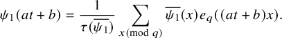 $$ \begin{align*} \psi_{1}(at+b) = \frac{1}{\tau(\overline{\psi_{1}})} \sum_{x \pmod{q} } \overline{\psi_{1}}(x) e_{q}((at+b)x). \end{align*} $$
We would like to calculate the t-sum to reduce the problem to the manipulation of the x-sum. Then
 $$ \begin{align*} \sum_{t \pmod{q} } \psi_{2}(ct+d) e_{q}(atx) = \sum_{t \pmod{q} } \psi_{2}(t) e_{q}(a \overline{c}(t-d)x) = \overline{\psi_{2}}(ax) \psi_{2}(c) e_{q}(-a \overline{c} dx) \tau(\psi_{2}). \end{align*} $$
On the other hand, one has
 $$ \begin{align*} \sum_{x \pmod{q} } \overline{\psi_{1} \psi_{2}}(x) e_{q}(x(b-a \overline{c} d)) = \psi_{1} \psi_{2}(ad-bc) \overline{\psi_{1} \psi_{2}}(-c) \tau(\overline{\psi_{1} \psi_{2}}). \end{align*} $$
Gathering the above identities together, we arrive at
 $$ \begin{align*} \sum_{t \pmod{q} } \psi_{1}(at+b) \psi_{2}(ct+d) = \overline{\psi_{1}}(c) \overline{\psi_{2}}(a) \psi_{1} \psi_{2}(bc-ad) \frac{\tau(\psi_{2}) \tau(\overline{\psi_{1} \psi_{2}})}{\tau(\overline{\psi_{1}})}. \end{align*} $$
Applying the relations $\tau (\overline {\psi _{1}}) = \psi _{1}(-1) \tau (\psi _{1})^{-1} q$
and
$\tau (\overline {\psi _{1}}) = \psi _{1}(-1) \tau (\psi _{1})^{-1} q$
and $\tau (\psi _{2}) = \psi _{2}(-1) \tau (\overline {\psi _{2}})^{-1} q$
, the desired expression follows. The second claim is the same as in [Reference Petrow and Young64, Lemma 6.3].
$\tau (\psi _{2}) = \psi _{2}(-1) \tau (\overline {\psi _{2}})^{-1} q$
, the desired expression follows. The second claim is the same as in [Reference Petrow and Young64, Lemma 6.3].
As mentioned in the introduction, we will encounter sums of the product of Kloosterman sums. One should resolve $\overline {\ell }$
inside the argument of the Kloosterman sum, and the following lemma is helpful when we expand
$\overline {\ell }$
inside the argument of the Kloosterman sum, and the following lemma is helpful when we expand $S(a \overline {\ell }, \pm n \overline {\ell }; q)$
into multiplicative characters.
$S(a \overline {\ell }, \pm n \overline {\ell }; q)$
into multiplicative characters.
Lemma 2.3. Assume that $q \geqslant 1$
and
$q \geqslant 1$
and $a, b \in \mathbb {Z}$
. We write
$a, b \in \mathbb {Z}$
. We write $a = a_{0} a^{\prime }$
and
$a = a_{0} a^{\prime }$
and $b = b_{0} b^{\prime }$
, where
$b = b_{0} b^{\prime }$
, where $a_{0} b_{0} \mid q^{\infty }$
and
$a_{0} b_{0} \mid q^{\infty }$
and $(a^{\prime } b^{\prime }, q) = 1$
. Then
$(a^{\prime } b^{\prime }, q) = 1$
. Then
 $$ \begin{align} S(a, b; q) = \frac{1}{\varphi(q)} \sum_{\psi \pmod{q} } \tau(\psi, a_{0}) \tau(\psi, b_{0}) \overline{\psi}(a^{\prime} b^{\prime}), \end{align} $$
where the sum runs over all Dirichlet characters modulo q and $\varphi (q)$
is Euler’s totient function.
$\varphi (q)$
is Euler’s totient function.
Proof. We exploit equation (2.3) so that the Kloosterman sum $S(a, b; q)$
equals
$S(a, b; q)$
equals
 $$ \begin{align*} \sideset{}{^{\ast}} \sum_{d\! \pmod{q} } e \left(\frac{a_{0} d+b_{0} a^{\prime} b^{\prime} \overline{d}}{q} \right) & = \frac{1}{\varphi(q)} \ \sideset{}{^{\ast}} \sum_{d\! \pmod{q} } e \left(\frac{a_{0} d}{q} \right) \sum_{\psi \pmod{q} } \overline{\psi}(a^{\prime} b^{\prime} \overline{d}) \tau(\psi, b_{0})\\ & = \frac{1}{\varphi(q)} \sum_{\psi \pmod{q} } \tau(\psi, a_{0}) \tau(\psi, b_{0}) \overline{\psi}(a^{\prime} b^{\prime}). \end{align*} $$
This finishes the proof of the lemma.
Direct corollaries of Lemma 2.3 include
Corollary 2.4. Suppose that $q \geqslant 1$
and
$q \geqslant 1$
and $a, b \in \mathbb {Z}$
. For
$a, b \in \mathbb {Z}$
. For $(ab, q) = 1$
, we then have
$(ab, q) = 1$
, we then have
 $$ \begin{align*} S(a, b; q) = \frac{1}{\varphi(q)} \sum_{\psi \pmod{q} } \tau(\psi)^{2} \overline{\psi}(ab). \end{align*} $$
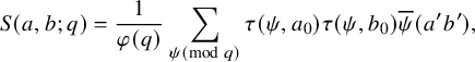
This idea of separation of variables traces back to celebrated work of Blomer–Milićević in [Reference Blomer and Milićević15]. The number of the Gauß sums is the crux in Lemma 2.3 as the nth power determines the hyper-Kloosterman sum of n variables. A variation of Lemma 2.3 was employed by Petrow–Young [Reference Petrow and Young64, Lemma 8.8], where they handled the hyper-Kloosterman sum $\mathrm {Kl}_{3}(x, y, z; q)$
.
$\mathrm {Kl}_{3}(x, y, z; q)$
.
2.2 Double Estermann zeta function
We introduce the divisor function
 $$ \begin{align*} \sigma_{w}(m) = \sum_{d \mid m} d^{w}. \end{align*} $$
As far as we know, the proof of the Hecke relation for $\sigma _{w}(m)$
has not appeared in the antecedent literature.
$\sigma _{w}(m)$
has not appeared in the antecedent literature.
Lemma 2.5. The divisor function satisfies the following multiplicativity relation:
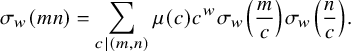 $$ \begin{align} \sigma_{w}(mn) = \sum_{c \mid (m, n)} \mu(c) c^{w} \sigma_{w} \left(\frac{m}{c} \right) \sigma_{w} \left(\frac{n}{c} \right). \end{align} $$
Proof. If $m = p_{1}^{k_{1}} p_{2}^{k_{2}} \cdots p_{r}^{k_{r}}$
,
$m = p_{1}^{k_{1}} p_{2}^{k_{2}} \cdots p_{r}^{k_{r}}$
, $n = p_{1}^{\ell _{1}} p_{2}^{\ell _{2}} \cdots p_{r}^{\ell _{r}}$
and such a formula is shown for powers of primes, then
$n = p_{1}^{\ell _{1}} p_{2}^{\ell _{2}} \cdots p_{r}^{\ell _{r}}$
and such a formula is shown for powers of primes, then
 $$ \begin{align} \begin{split} \sigma_{w}(mn) &= \sigma_{w}(p_{1}^{k_{1}+\ell_{1}}) \sigma_{w}(p_{2}^{k_{2}+\ell_{2}}) \cdots \sigma_{w}(p_{r}^{k_{r}+\ell_{r}})\\ & = \prod_{i = 1}^{r} \sum_{j = 0}^{\min(k_{i}, \ell_{i})} \mu(p_{i}^{j}) p_{i}^{jw} \sigma_{w}(p_{i}^{k_{i}-j}) \sigma_{w}(p_{i}^{\ell_{i}-j})\\ & = \sum_{c \mid (m, n)} \mu(c) c^{w} \sigma_{w} \left(\frac{m}{c} \right) \sigma_{w} \left(\frac{n}{c} \right). \end{split} \end{align} $$
By multiplicativity, it suffices to prove the result for $m = p^{k}$
,
$m = p^{k}$
, $n = p^{\ell }$
. The formula is obvious if
$n = p^{\ell }$
. The formula is obvious if $\min (k, \ell ) = 0$
, so we assume both the variables are at least
$\min (k, \ell ) = 0$
, so we assume both the variables are at least $1$
. Setting
$1$
. Setting $X = p^{w}$
, we find that the right-hand side of equation (2.11) reads
$X = p^{w}$
, we find that the right-hand side of equation (2.11) reads
 $$ \begin{align*} \text{RHS} &= \sigma_{w}(p^{k}) \sigma_{w}(p^{\ell})-p^{w} \sigma_{w}(p^{k-1}) \sigma_{w}(p^{\ell-1})\\ & = (1+X+\cdots+X^{k})(1+X+\cdots+X^{\ell})-X(1+X+\cdots+X^{k-1})(1+X+\cdots+X^{\ell-1})\\ & = \frac{X^{k+\ell+1}-1}{X-1} = (1+p^{w}+p^{2w}+\cdots+p^{(k+\ell)w}) = \sigma_{w}(p^{k+\ell}). \end{align*} $$
This establishes Lemma 2.5.
For positive integers $h, \ell $
with
$h, \ell $
with $(h, \ell ) = 1$
and
$(h, \ell ) = 1$
and $\Re (s)> 1$
, we define the double Estermann zeta function as
$\Re (s)> 1$
, we define the double Estermann zeta function as
 $$ \begin{align} D_{2} \left(s, \lambda; \frac{h}{\ell} \right) = \sum_{n = 1}^{\infty} \sigma_{\lambda}(n) e \left(\frac{nh}{\ell} \right) n^{-s}. \end{align} $$
Most of the analytic properties of $D_{2}(s, \lambda; h/\ell )$
follow from the identity
$D_{2}(s, \lambda; h/\ell )$
follow from the identity
 $$ \begin{align*} D_{2} \left(s, \lambda; \frac{h}{\ell} \right) = \ell^{\lambda-2s} \sum_{a, b\! \pmod{\ell}} e \left(\frac{abh}{\ell} \right) \zeta \left(s, \frac{a}{\ell} \right) \zeta \left(s-\lambda, \frac{b}{\ell} \right), \end{align*} $$
where for $\alpha \in \mathbb {R}$
and
$\alpha \in \mathbb {R}$
and $\Re (s)> 1$
,
$\Re (s)> 1$
,
is the Hurwitz zeta function. It has meromorphic continuation to the entire complex plane $\mathbb {C}$
with a simple pole at
$\mathbb {C}$
with a simple pole at $s = 1$
of residue 1 and satisfies the functional equation
$s = 1$
of residue 1 and satisfies the functional equation
 $$ \begin{align} \zeta(s, \alpha) = \sum_{\pm} G^{\mp}(1-s) \zeta^{(\pm \alpha)}(1-s), \end{align} $$
where $G^{\pm }(s) = (2\pi )^{-s} \Gamma (s) e(\pm s/4)$
and
$G^{\pm }(s) = (2\pi )^{-s} \Gamma (s) e(\pm s/4)$
and $\zeta ^{(\alpha )}(s)$
is a meromorphic continuation of
$\zeta ^{(\alpha )}(s)$
is a meromorphic continuation of $\sum _{n \geqslant 1} e(\alpha n) n^{-s}$
. For
$\sum _{n \geqslant 1} e(\alpha n) n^{-s}$
. For $\alpha \in \mathbb {Q}$
, the formula in equation (2.13) is a restatement of the Poisson summation in residue classes. Hence, as a function of the single variable s, the Estermann zeta function in equation (2.12) also has meromorphic continuation to all
$\alpha \in \mathbb {Q}$
, the formula in equation (2.13) is a restatement of the Poisson summation in residue classes. Hence, as a function of the single variable s, the Estermann zeta function in equation (2.12) also has meromorphic continuation to all $s \in \mathbb {C}$
with two simple poles at
$s \in \mathbb {C}$
with two simple poles at $s = 1$
and
$s = 1$
and $s = 1+\lambda $
with respective residues
$s = 1+\lambda $
with respective residues $\ell ^{\lambda -1} \zeta (1-\lambda )$
and
$\ell ^{\lambda -1} \zeta (1-\lambda )$
and $\ell ^{-\lambda -1} \zeta (1+\lambda )$
, provided
$\ell ^{-\lambda -1} \zeta (1+\lambda )$
, provided $\lambda \ne 0$
. In the case of
$\lambda \ne 0$
. In the case of $\lambda = 0$
, there is a double pole at
$\lambda = 0$
, there is a double pole at $s = 1$
, and the Laurent expansion is given by
$s = 1$
, and the Laurent expansion is given by
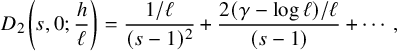 $$ \begin{align*} D_{2} \left(s, 0; \frac{h}{\ell} \right) = \frac{1/\ell}{(s-1)^{2}}+\frac{2(\gamma-\log \ell)/\ell}{(s-1)}+\cdots, \end{align*} $$
where $\gamma $
is the Euler–Mascheroni constant. The functional equation for
$\gamma $
is the Euler–Mascheroni constant. The functional equation for $D_{2}(s, \lambda; h/\ell )$
reads as follows:
$D_{2}(s, \lambda; h/\ell )$
reads as follows:
Theorem 2.6 ([Reference Motohashi55, Lemma 3.7])
The Estermann zeta function satisfies the functional equation
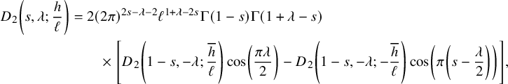 $$ \begin{align} D_{2} \left(s, \lambda; \frac{h}{\ell} \right) &= 2(2\pi)^{2s-\lambda-2} \ell^{1+\lambda-2s} \Gamma(1-s) \Gamma(1+\lambda-s) \notag \\ & \qquad \times \left[D_{2} \left(1-s, -\lambda; \frac{\overline{h}}{\ell} \right) \cos \left(\frac{\pi \lambda}{2} \right) - D_{2} \left(1-s, -\lambda; -\frac{\overline{h}}{\ell} \right) \cos \left(\pi \left(s-\frac{\lambda}{2} \right) \right) \right], \end{align} $$
where $\overline {h}$
is the multiplicative inverse of h modulo
$\overline {h}$
is the multiplicative inverse of h modulo $\ell $
: that is,
$\ell $
: that is, $h \overline {h} \equiv 1 \pmod {\ell }$
.
$h \overline {h} \equiv 1 \pmod {\ell }$
.
The formula in equation (2.14) was first proven by Hecke and Estermann in connection with an integral representation of the Hurwitz zeta function. We already find fragments of the Kloosterman sum in equation (2.14), which incline us to apply the Kloosterman summation formula. The functional equation of the Estermann zeta function $D_{2}$
is essentially equivalent to Voronoĭ summation. Indeed, the Estermann zeta function involves a divisor function instead of Hecke eigenvalues, and this corresponds to the standard Eisenstein series.
$D_{2}$
is essentially equivalent to Voronoĭ summation. Indeed, the Estermann zeta function involves a divisor function instead of Hecke eigenvalues, and this corresponds to the standard Eisenstein series.
2.3 Kloosterman sums at singular cusps
Our presentation of cusps and scaling matrices is inspired by [Reference Iwaniec37]. We restrict our attention to cusps with respect to the Hecke congruence subgroup

Let $q_{0} \mid q$
. In the following, the letter
$q_{0} \mid q$
. In the following, the letter $\psi $
denotes a Dirichlet character modulo
$\psi $
denotes a Dirichlet character modulo $q_{0}$
with
$q_{0}$
with $\kappa = (1-\psi (-1))/2$
such that
$\kappa = (1-\psi (-1))/2$
such that $\psi (-1) = (-1)^{\kappa }$
. Then we extend
$\psi (-1) = (-1)^{\kappa }$
. Then we extend $\psi $
via the identification
$\psi $
via the identification
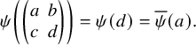 $$ \begin{align*} \psi \left(\begin{pmatrix} a & b \\ c & d \end{pmatrix} \right) = \psi(d) = \overline{\psi}(a). \end{align*} $$
The group $\Gamma $
acts transitively on
$\Gamma $
acts transitively on $\mathbb {P}^{1}(\mathbb {Q})$
by fractional linear transformations. An element
$\mathbb {P}^{1}(\mathbb {Q})$
by fractional linear transformations. An element $\mathfrak {a} \in \mathbb {P}^{1}(\mathbb {Q})$
is called a cusp. Two cusps
$\mathfrak {a} \in \mathbb {P}^{1}(\mathbb {Q})$
is called a cusp. Two cusps $\mathfrak {a}$
and
$\mathfrak {a}$
and $\mathfrak {b}$
are termed equivalent under
$\mathfrak {b}$
are termed equivalent under $\Gamma $
if there exists
$\Gamma $
if there exists $\gamma \in \Gamma $
satisfying
$\gamma \in \Gamma $
satisfying $\mathfrak {a} = \gamma \mathfrak {b}$
. We write
$\mathfrak {a} = \gamma \mathfrak {b}$
. We write $q = rs$
with
$q = rs$
with $(r, s) = 1$
and
$(r, s) = 1$
and $q_{0} \mid s$
. Then we call a cusp of the form
$q_{0} \mid s$
. Then we call a cusp of the form $\mathfrak {a} = 1/r$
an Atkin–Lehner cusp. The Atkin–Lehner cusps are equivalent to
$\mathfrak {a} = 1/r$
an Atkin–Lehner cusp. The Atkin–Lehner cusps are equivalent to $\infty $
under the Atkin–Lehner operator as in [Reference Kıral and Young46, Definition 2.4]. Motohashi [Reference Motohashi57] singled out the scaling matrices corresponding to the Atkin–Lehner operators and this is crucial since the Fourier coefficients around the cusp
$\infty $
under the Atkin–Lehner operator as in [Reference Kıral and Young46, Definition 2.4]. Motohashi [Reference Motohashi57] singled out the scaling matrices corresponding to the Atkin–Lehner operators and this is crucial since the Fourier coefficients around the cusp $1/r$
are proportional to the Fourier coefficients around the cusp
$1/r$
are proportional to the Fourier coefficients around the cusp $\infty $
for an eigenform of the Atkin–Lehner operators.
$\infty $
for an eigenform of the Atkin–Lehner operators.
Let $\Gamma _{\mathfrak {a}} = \{\gamma \in \Gamma : \gamma \mathfrak {a} = \mathfrak {a} \}$
be the stabiliser of the cusp
$\Gamma _{\mathfrak {a}} = \{\gamma \in \Gamma : \gamma \mathfrak {a} = \mathfrak {a} \}$
be the stabiliser of the cusp $\mathfrak {a}$
in
$\mathfrak {a}$
in $\Gamma $
. A matrix
$\Gamma $
. A matrix $\sigma _{\mathfrak {a}} \in \textrm{SL}_{2}(\mathbb {R})$
, satisfying
$\sigma _{\mathfrak {a}} \in \textrm{SL}_{2}(\mathbb {R})$
, satisfying
 $$ \begin{align*} \sigma_{\mathfrak{a}} \infty = \mathfrak{a} \quad \text{and} \quad \sigma_{\mathfrak{a}}^{-1} \Gamma_{\mathfrak{a}} \sigma_{\mathfrak{a}} = \Gamma_{\infty} = \left\{\pm \begin{pmatrix} 1 & n \\ 0 & 1 \end{pmatrix}: n \in \mathbb{Z} \right\} \end{align*} $$
is called a scaling matrix for the cusp $\mathfrak {a}$
. Since the scaling matrix
$\mathfrak {a}$
. Since the scaling matrix $\sigma _{\mathfrak {a}}$
is not uniquely determined, the choice of
$\sigma _{\mathfrak {a}}$
is not uniquely determined, the choice of $\sigma _{\mathfrak {a}}$
will be important in our subsequent discussions.
$\sigma _{\mathfrak {a}}$
will be important in our subsequent discussions.
Definition 2.7. Let $\mathfrak {a}, \mathfrak {b}$
be cusps and
$\mathfrak {a}, \mathfrak {b}$
be cusps and $\sigma _{\mathfrak {a}}, \sigma _{\mathfrak {b}}$
be scaling matrices. The set
$\sigma _{\mathfrak {a}}, \sigma _{\mathfrak {b}}$
be scaling matrices. The set
 $$ \begin{align*} \mathcal{C}(\mathfrak{a}, \mathfrak{b}) = \left\{{c}> 0: \begin{pmatrix} \ast & \ast \\ {c} & \ast \end{pmatrix} \in \sigma_{\mathfrak{a}}^{-1} \Gamma \sigma_{\mathfrak{b}} \right\} \end{align*} $$
is called the set of allowed moduli.
For a cusp $\mathfrak {a}$
and a scaling matrix
$\mathfrak {a}$
and a scaling matrix $\sigma _{\mathfrak {a}}$
, let
$\sigma _{\mathfrak {a}}$
, let $u_{\mathfrak {a}}$
be such that
$u_{\mathfrak {a}}$
be such that $\sigma _{\mathfrak {a}}^{-1} u_{\mathfrak {a}} \sigma _{\mathfrak {a}} = \left (\begin {smallmatrix} 1 & 1 \\ & 1 \end {smallmatrix} \right )$
. If
$\sigma _{\mathfrak {a}}^{-1} u_{\mathfrak {a}} \sigma _{\mathfrak {a}} = \left (\begin {smallmatrix} 1 & 1 \\ & 1 \end {smallmatrix} \right )$
. If $\psi $
satisfies
$\psi $
satisfies $\psi (u_{\mathfrak {a}}) = 1$
, then we say that
$\psi (u_{\mathfrak {a}}) = 1$
, then we say that $\mathfrak {a}$
is singular with respect to
$\mathfrak {a}$
is singular with respect to $\psi $
. It behooves one to mention the following proposition:
$\psi $
. It behooves one to mention the following proposition:
Proposition 2.8 ([Reference Kıral and Young46, Proposition 2.6])
Assume that $q = rs$
with
$q = rs$
with $(r, s) = 1$
with
$(r, s) = 1$
with $q_{0} \mid s$
, where
$q_{0} \mid s$
, where $q_{0}$
is the modulus of
$q_{0}$
is the modulus of $\psi $
. The two cusps
$\psi $
. The two cusps $\infty $
and
$\infty $
and $1/r$
are then singular with respect to
$1/r$
are then singular with respect to $\psi $
. We choose a scaling matrix
$\psi $
. We choose a scaling matrix $\sigma _{1/r}$
associated to the Atkin–Lehner cusp
$\sigma _{1/r}$
associated to the Atkin–Lehner cusp $1/r$
to be an Atkin–Lehner operator, namely
$1/r$
to be an Atkin–Lehner operator, namely
 $$ \begin{align*} \sigma_{1/r} = \tau_{r} \nu_{s} \quad \text{with} \quad \tau_{r} = \begin{pmatrix} 1 & (s \overline{s}-1)/r \\ r & s \overline{s} \end{pmatrix}, \quad \nu_{s} = \begin{pmatrix} \sqrt{s} & \\ & 1/\sqrt{s} \end{pmatrix} \end{align*} $$
with $s \overline {s} \equiv 1 \pmod {r}$
. Then the set of allowed moduli is given by
$s \overline {s} \equiv 1 \pmod {r}$
. Then the set of allowed moduli is given by
 $$ \begin{align*} \mathcal{C}(\infty, 1/r) = \{\gamma = c \sqrt{s}: c \equiv 0 \pmod{r}, \ (c, s) = 1 \}. \end{align*} $$
An important example is when $r = 1$
and
$r = 1$
and $s = q$
. In this case, one has
$s = q$
. In this case, one has
 $$ \begin{align*} \mathcal{C}(\infty, 0) = \{c \sqrt{q}: c \geqslant 1, \ (c, q) = 1 \}. \end{align*} $$
We now define Kloosterman sums with respect to a pair of cusps and general central character.
Definition 2.9. If $\mathfrak {a}, \mathfrak {b}$
are singular cusps for
$\mathfrak {a}, \mathfrak {b}$
are singular cusps for $\psi $
modulo
$\psi $
modulo $q_{0}$
, then the Kloosterman sum associated to
$q_{0}$
, then the Kloosterman sum associated to $\mathfrak {a}$
,
$\mathfrak {a}$
, $\mathfrak {b}$
and
$\mathfrak {b}$
and $\psi $
with modulus c is defined as
$\psi $
with modulus c is defined as
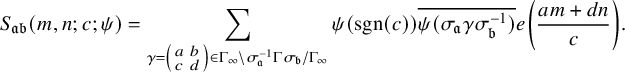 $$ \begin{align} S_{\mathfrak{ab}}(m, n; c; \psi) = \sum_{\gamma = \left(\begin{smallmatrix} a & b \\ c & d \end{smallmatrix} \right) \in \Gamma_{\infty} \backslash \sigma_{\mathfrak{a}}^{-1} \Gamma \sigma_{\mathfrak{b}}/\Gamma_{\infty}} \psi(\mathrm{sgn}(c)) \overline{\psi(\sigma_{\mathfrak{a}} \gamma \sigma_{\mathfrak{b}}^{-1})} e \left(\frac{am+dn}{c} \right). \end{align} $$
The occurrence of $-I \in \Gamma _{\infty }$
indicates that the lower-left entry c is only defined up to
$-I \in \Gamma _{\infty }$
indicates that the lower-left entry c is only defined up to $\pm $
sign, so that the factor
$\pm $
sign, so that the factor $\psi (\mathrm {sgn}(c))$
accounts for this. Definition 2.9 is sensitively dependent upon the choice of
$\psi (\mathrm {sgn}(c))$
accounts for this. Definition 2.9 is sensitively dependent upon the choice of $\sigma _{\mathfrak {a}}$
and
$\sigma _{\mathfrak {a}}$
and $\sigma _{\mathfrak {b}}$
. Moreover, if
$\sigma _{\mathfrak {b}}$
. Moreover, if $|c| \notin \mathcal {C}(\mathfrak {a}, \mathfrak {b})$
, then the sum appearing in equation (2.15) is empty, thus
$|c| \notin \mathcal {C}(\mathfrak {a}, \mathfrak {b})$
, then the sum appearing in equation (2.15) is empty, thus $S_{\mathfrak {ab}}(m, n; c; \psi ) = 0$
. If we stick to the case of
$S_{\mathfrak {ab}}(m, n; c; \psi ) = 0$
. If we stick to the case of $\mathfrak {a} = \infty $
and
$\mathfrak {a} = \infty $
and $\mathfrak {b} = 0$
, we know the identity (see [Reference Kıral and Young46, (2.20)])
$\mathfrak {b} = 0$
, we know the identity (see [Reference Kıral and Young46, (2.20)])
 $$ \begin{align} S_{\infty 0}(m, n; c \sqrt{q}; \psi) = \overline{\psi}(c) S(m, n \overline{q}; c) \end{align} $$
with $(c, q) = 1$
and
$(c, q) = 1$
and $q \overline {q} \equiv 1 \pmod {c}$
. This differs from the one shown in [Reference Iwaniec36, Page 58] by an additive character, which is due to a different choice of the scaling matrix. In the formula in equation (2.16), the presence of the character
$q \overline {q} \equiv 1 \pmod {c}$
. This differs from the one shown in [Reference Iwaniec36, Page 58] by an additive character, which is due to a different choice of the scaling matrix. In the formula in equation (2.16), the presence of the character $\overline {\psi }(c)$
is a nice feature of the
$\overline {\psi }(c)$
is a nice feature of the $(\infty , 0)$
cusp-pair as opposed to the
$(\infty , 0)$
cusp-pair as opposed to the $(\infty , \infty )$
cusp-pair:
$(\infty , \infty )$
cusp-pair:
 $$ \begin{align} S_{\infty \infty}(m, n; c; \psi) = S_{\psi}(m, n; c) = \sideset{}{^{\ast}} \sum_{d\! \pmod{c} } \psi(d) e \left(\frac{md+n \overline{d}}{c} \right). \end{align} $$
2.4 Normalisation and Hecke eigenvalues
In order to formulate our Kloosterman summation formula, we borrow the normalisation from [Reference Blomer, Harcos and Michel9, Reference Duke, Friedlander and Iwaniec23]. We refer the reader to [Reference Proskurin65] for an exposition in the case of general multiplier systems. Let $\Gamma \backslash \mathbb {H}$
be the modular surface, where
$\Gamma \backslash \mathbb {H}$
be the modular surface, where $\Gamma = \Gamma _{0}(q)$
is the Hecke congruence subgroup and
$\Gamma = \Gamma _{0}(q)$
is the Hecke congruence subgroup and $\mathbb {H} = \{z \in \mathbb {C}: \Im (z)> 0 \}$
is the upper half-plane. There exist various self-adjoint and pairwise commuting operators acting on the space
$\mathbb {H} = \{z \in \mathbb {C}: \Im (z)> 0 \}$
is the upper half-plane. There exist various self-adjoint and pairwise commuting operators acting on the space $L^{2}(\Gamma \backslash \mathbb {H})$
: the hyperbolic Laplacian
$L^{2}(\Gamma \backslash \mathbb {H})$
: the hyperbolic Laplacian
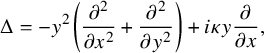 $$ \begin{align*} \Delta = -y^{2} \left(\frac{\partial^{2}}{\partial x^{2}}+\frac{\partial^{2}}{\partial y^{2}} \right)+i\kappa y \frac{\partial}{\partial x}, \end{align*} $$
the Hecke operators (the non-archimedean counterparts of $\Delta $
)
$\Delta $
)
 $$ \begin{align} (T_{n} f)(z) = \frac{1}{\sqrt{n}} \sum_{ad = n} \psi(a) \sum_{b\! \pmod{d}} f \left(\frac{az+b}{d} \right), \end{align} $$
and the reflection operator $(T_{-1} f)(z) = f(-\overline {z})$
, which flips positive and negative Fourier coefficients. As shall be explained later, we have the spectral decomposition of
$(T_{-1} f)(z) = f(-\overline {z})$
, which flips positive and negative Fourier coefficients. As shall be explained later, we have the spectral decomposition of $L^{2}(\Gamma \backslash \mathbb {H})$
in terms of pure point spectrum, residual spectrum and continuous spectrum, namely
$L^{2}(\Gamma \backslash \mathbb {H})$
in terms of pure point spectrum, residual spectrum and continuous spectrum, namely
 $$ \begin{align*} L^{2}(\Gamma \backslash \mathbb{H}) = L_{\text{cusp}}^{2}(\Gamma \backslash \mathbb{H}) \oplus L_{\text{res}}^{2}(\Gamma \backslash \mathbb{H}) \oplus L_{\text{cont}}^{2}(\Gamma \backslash \mathbb{H}). \end{align*} $$
For an integer $k> 0$
with
$k> 0$
with $k \equiv \kappa \pmod {2}$
, we choose a basis
$k \equiv \kappa \pmod {2}$
, we choose a basis $\mathcal {B}_{k}(q, \psi )$
of holomorphic cusp forms. It is taken orthonormal with respect to the weight k Petersson inner product
$\mathcal {B}_{k}(q, \psi )$
of holomorphic cusp forms. It is taken orthonormal with respect to the weight k Petersson inner product
 $$ \begin{align} \langle h_{1}, h_{2} \rangle = \int_{\Gamma \backslash \mathbb{H}} h_{1}(z) \overline{h_{2}(z)} y^{k} \frac{dx dy}{y^{2}}, \end{align} $$
where $z = x+iy$
. We let
$z = x+iy$
. We let $\mathcal {B}_{\kappa }(q, \psi )$
denote a basis of the space of Maaß cusp forms. In particular, they are eigenfunctions on
$\mathcal {B}_{\kappa }(q, \psi )$
denote a basis of the space of Maaß cusp forms. In particular, they are eigenfunctions on $\mathbb {H}$
, are automorphic of weight
$\mathbb {H}$
, are automorphic of weight $\kappa \in \{0, 1 \}$
, are square-integrable on a fundamental domain and vanish at all the cusps. Moreover, they are eigenfunctions of the
$\kappa \in \{0, 1 \}$
, are square-integrable on a fundamental domain and vanish at all the cusps. Moreover, they are eigenfunctions of the $L^{2}$
-extension of the hyperbolic Laplacian
$L^{2}$
-extension of the hyperbolic Laplacian $\Delta $
. For
$\Delta $
. For $f \in \mathcal {B}_{\kappa }(q, \psi )$
, we write
$f \in \mathcal {B}_{\kappa }(q, \psi )$
, we write $\Delta f = s(1-s)f$
with
$\Delta f = s(1-s)f$
with $s = 1/2+it_{f}$
and
$s = 1/2+it_{f}$
and $t_{f} \in \mathbb {R} \cup i[-1/2, 1/2]$
. One may choose the basis
$t_{f} \in \mathbb {R} \cup i[-1/2, 1/2]$
. One may choose the basis $\mathcal {B}_{\kappa }(q, \psi )$
orthonormal with respect to the weight zero Petersson inner product introduced above. We define
$\mathcal {B}_{\kappa }(q, \psi )$
orthonormal with respect to the weight zero Petersson inner product introduced above. We define
Then the Selberg eigenvalue conjecture asserts $\vartheta = 0$
, whereas Selberg only established the upper bound
$\vartheta = 0$
, whereas Selberg only established the upper bound $\vartheta \leqslant 1/4$
. The current world record is
$\vartheta \leqslant 1/4$
. The current world record is $\vartheta \leqslant 7/64$
due to Kim–Sarnak [Reference Kim45] (see Blomer–Brumley [Reference Blomer and Brumley7] for the treatment in a more general scenario). The decomposition of the space of square-integrable, weight
$\vartheta \leqslant 7/64$
due to Kim–Sarnak [Reference Kim45] (see Blomer–Brumley [Reference Blomer and Brumley7] for the treatment in a more general scenario). The decomposition of the space of square-integrable, weight $\kappa $
automorphic forms on
$\kappa $
automorphic forms on $\mathbb {H}$
with respect to the eigenspaces of the hyperbolic Laplacian involves the Eisenstein spectrum
$\mathbb {H}$
with respect to the eigenspaces of the hyperbolic Laplacian involves the Eisenstein spectrum $\mathcal {E}(q, \psi )$
, which is the orthogonal complement to the space of Maaß cusp forms. It is explicitly described in terms of the Eisenstein series
$\mathcal {E}(q, \psi )$
, which is the orthogonal complement to the space of Maaß cusp forms. It is explicitly described in terms of the Eisenstein series $E_{\mathfrak {a}}(z, 1/2+it)$
, where
$E_{\mathfrak {a}}(z, 1/2+it)$
, where $\mathfrak {a}$
runs over singular cusps and
$\mathfrak {a}$
runs over singular cusps and $t \in \mathbb {R}$
. In this article, instead of using the classical Eisenstein series indexed by singular cusps as a basis of the continuous spectrum, we use another basis of Eisenstein series indexed by a set of parameters of the form
$t \in \mathbb {R}$
. In this article, instead of using the classical Eisenstein series indexed by singular cusps as a basis of the continuous spectrum, we use another basis of Eisenstein series indexed by a set of parameters of the form
 $$ \begin{align*} \{(\psi_{1}, \psi_{2}, f): \psi_{1} \psi_{2} = \psi, \, f \in \mathcal{B}(\psi_{1}, \psi_{2}) \}, \end{align*} $$
where $(\psi _{1}, \psi _{2})$
ranges over the pairs of characters of modulus q such that
$(\psi _{1}, \psi _{2})$
ranges over the pairs of characters of modulus q such that $\psi _{1} \psi _{2} = \psi $
and
$\psi _{1} \psi _{2} = \psi $
and $\mathcal {B}(\psi _{1}, \psi _{2})$
is a certain finite set dependent on
$\mathcal {B}(\psi _{1}, \psi _{2})$
is a certain finite set dependent on $(\psi _{1}, \psi _{2})$
. We do not need to be more explicit here, and we refer the reader to [Reference Gelbart, Jacquet, Borel and Casselman24] for an accurate definition of these parameters. The principal advantage of such a basis is that the Eisenstein series are eigenforms of the Hecke operators
$(\psi _{1}, \psi _{2})$
. We do not need to be more explicit here, and we refer the reader to [Reference Gelbart, Jacquet, Borel and Casselman24] for an accurate definition of these parameters. The principal advantage of such a basis is that the Eisenstein series are eigenforms of the Hecke operators $T_{n}$
with
$T_{n}$
with $(n, q) = 1$
: we have
$(n, q) = 1$
: we have
 $$ \begin{align*} T_{n} E(z, 1/2+it, f) = \lambda_{f}(n, t) E(z, 1/2+it, f) \end{align*} $$
with
 $$ \begin{align*} \lambda_{f}(n, t) = \sum_{ab = n} \psi_{1}(a) a^{it} \psi_{2}(b) b^{-it}. \end{align*} $$
For convenience, we introduce the ad hoc notation
 $$ \begin{align*} i(g, z) = cz+d, \qquad j(g, z) = (cz+d)|cz+d|^{-1}, \qquad g = \begin{pmatrix} \ast & \ast \\ c & d \end{pmatrix} \in \textrm{SL}_{2}(\mathbb{R}). \end{align*} $$
We write the Fourier expansion of $f \in \mathcal {B}_{k}(q, \psi )$
around a singular cusp
$f \in \mathcal {B}_{k}(q, \psi )$
around a singular cusp $\mathfrak {a}$
with a scaling matrix
$\mathfrak {a}$
with a scaling matrix $\sigma _{\mathfrak {a}}$
as
$\sigma _{\mathfrak {a}}$
as
 $$ \begin{align*} i(\sigma_{\mathfrak{a}}, z)^{-k} f(\sigma_{\mathfrak{a}} z) = \left(\frac{(4\pi)^{k}}{\Gamma(k)} \right)^{1/2} \sum_{n = 1}^{\infty} \rho_{f \mathfrak{a}}(n) n^{(k-1)/2} e(nz). \end{align*} $$
Let $f \in \mathcal {B}_{\kappa }(q, \psi )$
be an orthonormal basis of the space of Maaß cusp forms of weight
$f \in \mathcal {B}_{\kappa }(q, \psi )$
be an orthonormal basis of the space of Maaß cusp forms of weight $\kappa $
with respect to
$\kappa $
with respect to $\Gamma _{0}(q)$
and central character
$\Gamma _{0}(q)$
and central character $\psi $
. As is customary, we assume that each f is either even or odd depending on whether
$\psi $
. As is customary, we assume that each f is either even or odd depending on whether $T_{-1} f = f$
or
$T_{-1} f = f$
or $T_{-1} f = -f$
. If we denote the corresponding spectral parameter by
$T_{-1} f = -f$
. If we denote the corresponding spectral parameter by $t_{f}$
, we have
$t_{f}$
, we have
 $$ \begin{align*} j(\sigma_{\mathfrak{a}}, z)^{-\kappa} f(\sigma_{\mathfrak{a}} z) = \sqrt{\cosh(\pi t_{f})} \sum_{n \ne 0} \frac{\rho_{f \mathfrak{a}}(n)}{|n|^{1/2}} W_{\frac{n}{|n|} \frac{\kappa}{2}, it_{f}}(4\pi|n|y) e(nx) \end{align*} $$
with $W_{\alpha , \beta }$
the standard Whittaker function. For an Eisenstein series
$W_{\alpha , \beta }$
the standard Whittaker function. For an Eisenstein series $E(z, 1/2+it, f)$
, we write
$E(z, 1/2+it, f)$
, we write
 $$ \begin{align*} j(\sigma_{\mathfrak{a}}, z)^{-\kappa} E(\sigma_{\mathfrak{a}} z, 1/2+it, f) &= c_{1, f, \mathfrak{a}}(t) y^{1/2+it}+c_{2, f, \mathfrak{a}}(t) y^{1/2-it}\\ &\qquad\qquad\qquad \ \ + \sqrt{\cosh(\pi t)} \sum_{n \ne 0} \frac{\rho_{f \mathfrak{a}}(n, t)}{|n|^{1/2}} W_{\frac{n}{|n|} \frac{\kappa}{2}, it}(4\pi |n|y) e(nx). \end{align*} $$
Now let $\mathcal {B}_{\kappa }^{\ast }(q, \psi )$
be an orthonormal basis consisting of Hecke–Maaß newforms of level q and central character
$\mathcal {B}_{\kappa }^{\ast }(q, \psi )$
be an orthonormal basis consisting of Hecke–Maaß newforms of level q and central character $\psi \pmod {q_{0}}$
normalised so that
$\psi \pmod {q_{0}}$
normalised so that $\lambda _{f}(1) = 1$
, and we define similarly
$\lambda _{f}(1) = 1$
, and we define similarly $\mathcal {B}_{k}^{\ast }(q, \psi )$
. By Atkin–Lehner–Li theory [Reference Atkin and Lehner2, Reference Atkin and Li3], we have the following direct sum decomposition as in [Reference Blomer and Milićević15]:
$\mathcal {B}_{k}^{\ast }(q, \psi )$
. By Atkin–Lehner–Li theory [Reference Atkin and Lehner2, Reference Atkin and Li3], we have the following direct sum decomposition as in [Reference Blomer and Milićević15]:
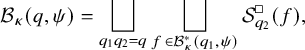 $$ \begin{align} \mathcal{B}_{\kappa}(q, \psi) = \bigsqcup_{q_{1} q_{2} = q} \bigsqcup_{f \in \mathcal{B}_{\kappa}^{\ast}(q_{1}, \psi)} \mathcal{S}_{q_{2}}^{\square}(f), \end{align} $$
where an element of the orthonormal basis $\mathcal {S}_{q_{2}}^{\square }(f) = \{f_{(d)}(z): d \mid q_{2} \}$
is written as a linear combination of
$\mathcal {S}_{q_{2}}^{\square }(f) = \{f_{(d)}(z): d \mid q_{2} \}$
is written as a linear combination of $f(cz)$
with
$f(cz)$
with $c \mid d$
. A description of this linear combination is given by Iwaniec–Luo–Sarnak [Reference Iwaniec, Luo and Sarnak39] for the squarefree level and principal nebentypus. Blomer–Milićević [Reference Blomer and Milićeić14] subsequently orthonormalised the collection of Maaß forms
$c \mid d$
. A description of this linear combination is given by Iwaniec–Luo–Sarnak [Reference Iwaniec, Luo and Sarnak39] for the squarefree level and principal nebentypus. Blomer–Milićević [Reference Blomer and Milićeić14] subsequently orthonormalised the collection of Maaß forms $\{f(dz): d \mid q_{2} \}$
for a newform f and an integer
$\{f(dz): d \mid q_{2} \}$
for a newform f and an integer $q_{2} \geqslant 1$
, which is not necessarily squarefree. Their scheme focuses on the principal nebentypus, but the generalisation to nontrivial central characters is feasible; see [Reference Humphries31]. There are the Atkin–Lehner–Li theory for the continuous spectrum and a decomposition into spaces of oldforms analogous to equation (2.20) due to Young [Reference Young70]. We make use of equation (2.20) to apply Hecke relations and the proportionality of Fourier coefficients to the Hecke eigenvalues.
$q_{2} \geqslant 1$
, which is not necessarily squarefree. Their scheme focuses on the principal nebentypus, but the generalisation to nontrivial central characters is feasible; see [Reference Humphries31]. There are the Atkin–Lehner–Li theory for the continuous spectrum and a decomposition into spaces of oldforms analogous to equation (2.20) due to Young [Reference Young70]. We make use of equation (2.20) to apply Hecke relations and the proportionality of Fourier coefficients to the Hecke eigenvalues.
In what follows, we make an abuse of notation $\rho _{f \infty }(n) = \rho _{f}(n)$
and
$\rho _{f \infty }(n) = \rho _{f}(n)$
and $\rho _{f \infty }(n, t) = \rho _{f}(n, t)$
. We consider the Fourier coefficients
$\rho _{f \infty }(n, t) = \rho _{f}(n, t)$
. We consider the Fourier coefficients $\rho _{f \mathfrak {a}}(n)$
in more detail, and we stick to the case of
$\rho _{f \mathfrak {a}}(n)$
in more detail, and we stick to the case of $\mathfrak {a} \sim \infty $
. Let
$\mathfrak {a} \sim \infty $
. Let $f \in \mathcal {B}_{\kappa }(q, \psi )$
be any Hecke eigenform, and let
$f \in \mathcal {B}_{\kappa }(q, \psi )$
be any Hecke eigenform, and let $\lambda _{f}(n)$
denote the corresponding eigenvalue for
$\lambda _{f}(n)$
denote the corresponding eigenvalue for $T_{n}$
, namely
$T_{n}$
, namely $T_{n} f = \lambda _{f}(n) f$
. Then we often use the Hecke multiplicativity relations for
$T_{n} f = \lambda _{f}(n) f$
. Then we often use the Hecke multiplicativity relations for $(mn, q) = 1$
:
$(mn, q) = 1$
:
 $$ \begin{align} \lambda_{f}(mn) = \sum_{d \mid (m, n)} \mu(d) \psi(d) \lambda_{f} \left(\frac{m}{d} \right) \lambda_{f} \left(\frac{n}{d} \right), \qquad \lambda_{f}(m) \lambda_{f}(n) = \sum_{d \mid (m, n)} \psi(d) \lambda_{f} \left(\frac{mn}{d^{2}} \right). \end{align} $$
We see some structural beauty of equation (2.21) in Section 3.5 along with the formula $\lambda _{f}(n) = \psi (n) \overline {\lambda _{f}(n)}$
for
$\lambda _{f}(n) = \psi (n) \overline {\lambda _{f}(n)}$
for $(n, q) = 1$
. Notice that the relation in equation (2.21) is valid for all
$(n, q) = 1$
. Notice that the relation in equation (2.21) is valid for all $m, n \geqslant 1$
if f is a newform. We invoke the bounds for the Hecke eigenvalues: if f belongs to
$m, n \geqslant 1$
if f is a newform. We invoke the bounds for the Hecke eigenvalues: if f belongs to $\mathcal {B}_{k}(q, \psi )$
or is an Eisenstein series, there follows that
$\mathcal {B}_{k}(q, \psi )$
or is an Eisenstein series, there follows that
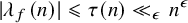 $$ \begin{align*} |\lambda_{f}(n)| \leqslant \tau(n) \ll_{\epsilon} n^{\epsilon} \end{align*} $$
for any $\epsilon> 0$
. For
$\epsilon> 0$
. For $f \in \mathcal {B}_{\kappa }(q, \psi )$
, the general upper bound is available in the form
$f \in \mathcal {B}_{\kappa }(q, \psi )$
, the general upper bound is available in the form
 $$ \begin{align} |\lambda_{f}(n)| \leqslant \tau(n) n^{\vartheta} \ll_{\epsilon} n^{\vartheta+\epsilon}. \end{align} $$
There is a connection between the Fourier coefficients and the Hecke eigenvalues
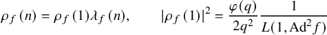 $$ \begin{align} \rho_{f}(n) = \rho_{f}(1) \lambda_{f}(n), \qquad |\rho_{f}(1)|^{2} = \frac{\varphi(q)}{2q^{2}} \frac{1}{L(1, \mathrm{Ad}^{2} f)} \end{align} $$
for $(n, q) = 1$
. We refer the reader to [Reference Duke, Friedlander and Iwaniec23, (6.14)] for the former and to [Reference Blomer6, (2.10)] for the latter. Here the adjoint square L-function is defined as
$(n, q) = 1$
. We refer the reader to [Reference Duke, Friedlander and Iwaniec23, (6.14)] for the former and to [Reference Blomer6, (2.10)] for the latter. Here the adjoint square L-function is defined as
 $$ \begin{align} L(s, \mathrm{Ad}^{2} f) = \zeta(2s) \sum_{n = 1}^{\infty} \frac{\lambda_{f}(n^{2})}{n^{s}}. \end{align} $$
The formula in equation (2.23) is valid for all $n \geqslant 1$
if f is a newform.
$n \geqslant 1$
if f is a newform.
Remark 2.10. If $\pi $
is an automorphic representation of
$\pi $
is an automorphic representation of $\operatorname {\mathrm {GL}}_{n}$
with a contradradient representation
$\operatorname {\mathrm {GL}}_{n}$
with a contradradient representation $\widetilde {\pi }$
, then it holds that
$\widetilde {\pi }$
, then it holds that $L(s, \widetilde {\pi }) = \overline {L(\overline {s}, \pi )}$
. In particular, the Dirichlet series coefficients of
$L(s, \widetilde {\pi }) = \overline {L(\overline {s}, \pi )}$
. In particular, the Dirichlet series coefficients of $L(s, \pi )$
are real if and only if
$L(s, \pi )$
are real if and only if $\pi \cong \widetilde {\pi }$
. If
$\pi \cong \widetilde {\pi }$
. If $n = 2$
, we have
$n = 2$
, we have $\widetilde {\pi } \cong \pi \otimes \omega ^{-1}$
, where
$\widetilde {\pi } \cong \pi \otimes \omega ^{-1}$
, where $\omega $
denotes the central character of
$\omega $
denotes the central character of $\pi $
. Hence the Hecke eigenvalues are not necessarily real in our context.
$\pi $
. Hence the Hecke eigenvalues are not necessarily real in our context.
The aforementioned formulæ for Hecke operators acting on holomorphic and Maaß cusp forms apply to the Eisenstein series since $\rho _{f}(n, t)$
are proportional to the Hecke eigenvalues
$\rho _{f}(n, t)$
are proportional to the Hecke eigenvalues $\lambda _{f}(n, t)$
(compare [Reference Duke, Friedlander and Iwaniec23, (7.13)]). We also derive the relation
$\lambda _{f}(n, t)$
(compare [Reference Duke, Friedlander and Iwaniec23, (7.13)]). We also derive the relation
 $$ \begin{align*} \rho_{f}(-n, t) = \frac{\Gamma(s+\kappa/2)}{\Gamma(s-\kappa/2)} \rho_{f}(n, t). \end{align*} $$
In Section 3, we are mainly interested in primitive Dirichlet characters $\psi ^{2}$
for primitive nonquadratic characters
$\psi ^{2}$
for primitive nonquadratic characters $\psi $
modulo a prime. In this case, one observes that
$\psi $
modulo a prime. In this case, one observes that $\kappa (\psi ^{2}) = 0$
, obtaining in particular that
$\kappa (\psi ^{2}) = 0$
, obtaining in particular that
 $$ \begin{align*} |\rho_{f}(n, t)|^{2} = \frac{|\lambda_{f}(n, t)|^{2}}{q|L(1+2it, \overline{\psi_{1}} \psi_{2})|^{2}}. \end{align*} $$
We also need to define the twisted automorphic L-function

which has meromorphic continuation to the whole complex plane $\mathbb {C}$
.
$\mathbb {C}$
.
2.5 A version of the Kuznetsov formula
A spectral summation formula that we deploy here is an asymmetric trace formula relating sums of Kloosterman sums to Fourier coefficients of automorphic forms in the sense that the spectral side and the geometric side have a quite different shape. This technology is able to establish that there are considerable cancellations in sums of Kloosterman sums. Moreover, it provides a separation of variables m and n in the sum $\sum _{c} S(m, n; c)/c$
, which is conducive to obtaining additional savings in summations over m and n.
$\sum _{c} S(m, n; c)/c$
, which is conducive to obtaining additional savings in summations over m and n.
For $x> 0$
, we introduce the three integral kernels
$x> 0$
, we introduce the three integral kernels

where we have borrowed the normalisation from [Reference Topaçoğullari67]. We decided to suppress $\psi $
from the notation, and we adopt this kind of abuse of notation unless otherwise specified. For
$\psi $
from the notation, and we adopt this kind of abuse of notation unless otherwise specified. For $F \in \mathcal {C}_{c}^{\infty }(\mathbb {R}_{+})$
, we introduce
$F \in \mathcal {C}_{c}^{\infty }(\mathbb {R}_{+})$
, we introduce
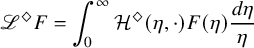 $$ \begin{align*} \mathscr{L}^{\Diamond} F = \int_{0}^{\infty} \mathcal{H}^{\Diamond}(\eta, \cdot) F(\eta) \frac{d\eta}{\eta} \end{align*} $$
for $\Diamond \in \{+, -, \mathrm {hol} \}$
. With the whole notation set up, we formulate the Kloosterman summation formula, which in our case reads as follows:
$\Diamond \in \{+, -, \mathrm {hol} \}$
. With the whole notation set up, we formulate the Kloosterman summation formula, which in our case reads as follows:
Theorem 2.11 ([Reference Topaçoğullari67, Theorem 3.2])
Assume $F \in C^{3}(0, \infty )$
satisfies
$F \in C^{3}(0, \infty )$
satisfies $x^{j} F^{(j)}(x) \ll \min (x, x^{-3/2})$
for
$x^{j} F^{(j)}(x) \ll \min (x, x^{-3/2})$
for $0 \leqslant j \leqslant 3$
. Let
$0 \leqslant j \leqslant 3$
. Let $\mathfrak {a}, \mathfrak {b}$
be singular cusps and
$\mathfrak {a}, \mathfrak {b}$
be singular cusps and $\psi \pmod {q_{0}}$
be a Dirichlet character, and let
$\psi \pmod {q_{0}}$
be a Dirichlet character, and let $m, n \geqslant 1$
. Then we have that
$m, n \geqslant 1$
. Then we have that
Here we set
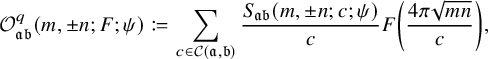


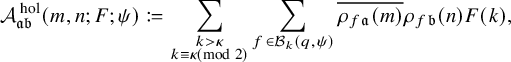
where the sum over c on the right-hand side of equation (2.26) runs over all positive real numbers for which the Kloosterman sum $S_{\mathfrak {ab}}(m, \pm n; c; \psi )$
is non-empty.
$S_{\mathfrak {ab}}(m, \pm n; c; \psi )$
is non-empty.
The above formulation mimics the Kuznetsov formula that Motohashi [Reference Motohashi55] utilised to show a spectral reciprocity for the smoothed fourth moment of the Riemann zeta function. The name of the Kloosterman summation formula stems from the fact that it expresses certain sums of Kloosterman sums weighted by a function F in terms of certain sums over automorphic forms weighted by transformed functions $\mathscr {L}^{\Diamond } F$
with
$\mathscr {L}^{\Diamond } F$
with $\Diamond \in \{+, -, \mathrm {hol} \}$
. We emphasise that there is no delta term in the Kloosterman summation formula.
$\Diamond \in \{+, -, \mathrm {hol} \}$
. We emphasise that there is no delta term in the Kloosterman summation formula.
3 Proof of Theorem 1.1
In this section, we prove Theorem 1.1 by applying the triad of Ramanujan–Voronoĭ–Kuznetsov to attack the shifted divisor sum in equation (1.14) for a primitive Dirichlet character $\chi $
modulo a prime q.
$\chi $
modulo a prime q.
3.1 Dissection argument of Atkinson
Recall equation (1.3) and Convention 1.10. Let $\mathcal {R}_{4}^{+}$
(respectively,
$\mathcal {R}_{4}^{+}$
(respectively, $\mathcal {R}_{4}^{-}$
) be the subdomain of
$\mathcal {R}_{4}^{-}$
) be the subdomain of $\mathbb {C}^{4}$
, where all four parameters have real parts larger than (respectively, less than) one. To wit, we define
$\mathbb {C}^{4}$
, where all four parameters have real parts larger than (respectively, less than) one. To wit, we define

For convenience, we write
for a vector $\texttt {s} = (s_{1}, s_{2}, s_{3}, s_{4})$
. In the domain
$\texttt {s} = (s_{1}, s_{2}, s_{3}, s_{4})$
. In the domain $\mathcal {R}_{4}^{+}$
, we open up the Dirichlet series to recast
$\mathcal {R}_{4}^{+}$
, we open up the Dirichlet series to recast $\mathcal {Z}_{2}$
as
$\mathcal {Z}_{2}$
as
 $$ \begin{align} \int_{-\infty}^{\infty} \sum_{n_{1} = 1}^{\infty} \sum_{n_{2} = 1}^{\infty} \sum_{n_{3} = 1}^{\infty} \sum_{n_{4} = 1}^{\infty} &\frac{\chi(n_{1}n_{2}) \overline{\chi}(n_{3} n_{4})}{n_{1}^{s_{1}} n_{2}^{s_{2}} n_{3}^{s_{3}} n_{4}^{s_{4}}} \left(\frac{n_{1}n_{2}}{n_{3} n_{4}} \right)^{-it} g(t) dt \notag \\[-2pt] &\qquad\qquad \quad \ = \sum_{m = 1}^{\infty} \sum_{n = 1}^{\infty} \frac{\chi(m) \overline{\chi}(n) \sigma_{s_{1}-s_{2}}(m) \sigma_{s_{3}-s_{4}}(n)}{m^{s_{1}} n^{s_{3}}} \hat{g} \left(\frac{1}{2\pi} \log \frac{m}{n} \right),\\[-16pt]\nonumber \end{align} $$
where $\hat {g}$
is the Fourier transformFootnote
4
$\hat {g}$
is the Fourier transformFootnote
4
 $$ \begin{align*} \hat{g}(\xi) = \int_{-\infty}^{\infty} g(t) e(-\xi t) dt.\\[-16pt] \end{align*} $$
Shifting the contour in equation (1.3) yields that $\mathcal {Z}_{2}$
is meromorphic over the domain
$\mathcal {Z}_{2}$
is meromorphic over the domain
 $$ \begin{align*} \mathcal{B}_{4} = \{(s_{1}, s_{2}, s_{3}, s_{4}) \in \mathbb{C}^{4}: |s_{1}|, |s_{2}|, |s_{3}|, |s_{4}| < B \},\\[-16pt] \end{align*} $$
where $B = cA$
and c is a small positive constant so that B is sufficiently large. Although it is possible to make B tend to infinity, we deal with the regime
$B = cA$
and c is a small positive constant so that B is sufficiently large. Although it is possible to make B tend to infinity, we deal with the regime $\mathcal {B}_{4}$
for technical convenience. Since we are assuming that
$\mathcal {B}_{4}$
for technical convenience. Since we are assuming that $\chi $
is primitive, the fourth moment
$\chi $
is primitive, the fourth moment $\mathcal {Z}_{2}$
is holomorphic in the vicinity of the point
$\mathcal {Z}_{2}$
is holomorphic in the vicinity of the point $\texttt {s} = (1/2, 1/2, 1/2, 1/2)$
. As an initial manipulation, we apply Atkinson’s dissection, decomposing the double sum in equation (3.1) into three parts. It therefore follows that
$\texttt {s} = (1/2, 1/2, 1/2, 1/2)$
. As an initial manipulation, we apply Atkinson’s dissection, decomposing the double sum in equation (3.1) into three parts. It therefore follows that
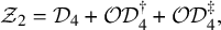 $$ \begin{align} \mathcal{Z}_{2} = \mathcal{D}_{4}+\mathcal{OD}_{4}^{\dagger}+\mathcal{OD}_{4}^{\ddagger},\\[-16pt]\nonumber \end{align} $$
where $\mathcal {D}_{4}$
is the diagonal contribution corresponding to the terms with
$\mathcal {D}_{4}$
is the diagonal contribution corresponding to the terms with $m = n$
, whereas
$m = n$
, whereas $\mathcal {OD}_{4}^{\dagger }$
(respectively,
$\mathcal {OD}_{4}^{\dagger }$
(respectively, $\mathcal {OD}_{4}^{\ddagger }$
) is the off-diagonal contribution corresponding to the terms with
$\mathcal {OD}_{4}^{\ddagger }$
) is the off-diagonal contribution corresponding to the terms with $m> n$
(respectively,
$m> n$
(respectively, $m < n$
). Note that the case of
$m < n$
). Note that the case of $m < n$
is symmetric to the case of
$m < n$
is symmetric to the case of $m> n$
as follows:
$m> n$
as follows:
 $$ \begin{align} \mathcal{OD}_{4}^{\ddagger}(s_{1}, s_{2}, s_{3}, s_{4}; g; \chi) = \overline{\mathcal{OD}_{4}^{\dagger}(\overline{s_{3}}, \overline{s_{4}}, \overline{s_{1}}, \overline{s_{2}}; g; \chi)}.\\[-16pt]\nonumber \end{align} $$
Breaking the summation in this manner leads one to certain sums of Kloosterman sums and ultimately to automorphic forms. For an explanation of the reason this is not as surprising as it initially seems, we refer the reader to the discussion in [Reference Motohashi55, §4.2].
Lemma 3.1. With the notation as above, we have that
 $$ \begin{align*} \mathcal{D}_{4} = \hat{g}(0) \frac{\zeta^{q}(s_{1}+s_{3}) \zeta^{q}(s_{1}+s_{4}) \zeta^{q}(s_{2}+s_{3}) \zeta^{q}(s_{2}+s_{4})}{\zeta^{q}(s_{1}+s_{2}+s_{3}+s_{4})},\\[-16pt] \end{align*} $$
where, for any L-function, the notation $L^{q}$
signifies the removal of the Euler factor at primes dividing q.
$L^{q}$
signifies the removal of the Euler factor at primes dividing q.
Proof. It suffices to calculate
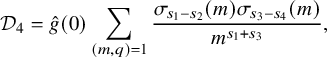 $$ \begin{align*} \mathcal{D}_{4} = \hat{g}(0) \sum_{(m, q) = 1} \frac{\sigma_{s_{1}-s_{2}}(m) \sigma_{s_{3}-s_{4}}(m)}{m^{s_{1}+s_{3}}},\\[-16pt] \end{align*} $$
where the Dirichlet series coefficient is a multiplicative function. Since the sum is over positive integers coprime to q, one can apply Ramanujan’s identity (see [Reference Hardy and Wright28, §17.8, Theorem 305])
 $$ \begin{align*} \sum_{m = 1}^{\infty} \frac{\sigma_{\alpha}(m) \sigma_{\beta}(m)}{m^{s}} = \frac{\zeta(s) \zeta(s-\alpha) \zeta(s-\beta) \zeta(s-\alpha-\beta)}{\zeta(2s-\alpha-\beta)},\\[-16pt] \end{align*} $$
omitting the Euler factors dividing q. This formula is valid as long as $\Re (s_{i})> 1/2$
.
$\Re (s_{i})> 1/2$
.
Note that $\hat {g}(0) = \int _{-\infty }^{\infty } g(t) dt$
is the mass of the weight function
$\hat {g}(0) = \int _{-\infty }^{\infty } g(t) dt$
is the mass of the weight function $\hat {g}_{T}(0) = T \hat {g}(0)$
, where
$\hat {g}_{T}(0) = T \hat {g}(0)$
, where $g_{T}(x) = g(x/T)$
with
$g_{T}(x) = g(x/T)$
with $T> 0$
. Hence, if g is compactly supported on the interval
$T> 0$
. Hence, if g is compactly supported on the interval $[1, 2]$
, then
$[1, 2]$
, then $\mathrm {supp}(g_{T}) \subseteq [T, 2T]$
. Since
$\mathrm {supp}(g_{T}) \subseteq [T, 2T]$
. Since $\mathcal {D}_{4}$
has a pole of order
$\mathcal {D}_{4}$
has a pole of order $4$
at
$4$
at $\texttt {s} = (1/2, 1/2, 1/2, 1/2)$
, we should have cancellation with a similar term coming from the off-diagonal terms. This is a common feature in the study of moment problems. The continuation of the off-diagonal contribution necessitates the full machinery of spectral theory of automorphic forms associated to Hecke congruence subgroups. We handle the second term in equation (3.2) due to the symmetry in equation (3.3), and the contribution from the third term will be incorporated at the end.
$\texttt {s} = (1/2, 1/2, 1/2, 1/2)$
, we should have cancellation with a similar term coming from the off-diagonal terms. This is a common feature in the study of moment problems. The continuation of the off-diagonal contribution necessitates the full machinery of spectral theory of automorphic forms associated to Hecke congruence subgroups. We handle the second term in equation (3.2) due to the symmetry in equation (3.3), and the contribution from the third term will be incorporated at the end.
3.2 Evaluation of off-diagonal terms
For notational convenience, we call
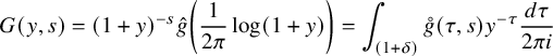 $$ \begin{align} G(y, s) = (1+y)^{-s} \hat{g} \left(\frac{1}{2\pi} \log(1+y) \right) = \int_{(1+\delta)} \mathring{g}(\tau, s) y^{-\tau} \frac{d\tau}{2\pi i} \end{align} $$
for suitable $\delta> 0$
, where
$\delta> 0$
, where $\mathring {g}$
is the Mellin transform
$\mathring {g}$
is the Mellin transform
 $$ \begin{align} \mathring{g}(\tau, s) = \int_{0}^{\infty} y^{\tau-1}(1+y)^{-s} \hat{g} \left(\frac{1}{2\pi} \log(1+y) \right) dy = \Gamma(\tau) \int_{-\infty}^{\infty} \frac{\Gamma(s-\tau+it)}{\Gamma(s+it)} g(t) dt, \end{align} $$
provided $\Re (s)> \Re (\tau ) > 0$
. The following lemma is useful:
$\Re (s)> \Re (\tau ) > 0$
. The following lemma is useful:
Lemma 3.2. As a function of two complex variables, $\mathring {g}(\tau , s)/\Gamma (\tau )$
is entire in
$\mathring {g}(\tau , s)/\Gamma (\tau )$
is entire in $\tau $
and s. In addition,
$\tau $
and s. In addition, $\mathring {g}(\tau , s)$
is of rapid decay in
$\mathring {g}(\tau , s)$
is of rapid decay in $\tau $
as long as s and
$\tau $
as long as s and $\Re (\tau )$
are bounded, say
$\Re (\tau )$
are bounded, say
 $$ \begin{align*} \mathring{g}(\tau, s) \ll (1+|\tau|)^{-A}. \end{align*} $$
Proof. Shifting the contour $\Im (t) = 0$
in equation (3.5) downward appropriately, we obtain the first assertion. The second claim is a consequence of an upward shift. See [Reference Motohashi55, Lemma 4.1] for an analogous statement.
$\Im (t) = 0$
in equation (3.5) downward appropriately, we obtain the first assertion. The second claim is a consequence of an upward shift. See [Reference Motohashi55, Lemma 4.1] for an analogous statement.
We now embark on the computation of $\mathcal {OD}_{4}^{\dagger }$
to resolve the shifted convolution problem. Pulling the Dirichlet characters out of the summations, one sees that
$\mathcal {OD}_{4}^{\dagger }$
to resolve the shifted convolution problem. Pulling the Dirichlet characters out of the summations, one sees that
 $$ \begin{align} \mathcal{OD}_{4}^{\dagger} = \sum_{a, b\!\! \pmod{q} } \overline{\chi}(a) \chi(a+b) \sum_{\substack{n \equiv a \pmod{q} \\ m \equiv b \pmod{q} }} \frac{\sigma_{s_{3}-s_{4}}(n) \sigma_{s_{1}-s_{2}}(n+m)}{n^{s_{1}+s_{3}}} G \left(\frac{m}{n}, s_{1} \right). \end{align} $$
We invoke the Ramanujan expansion (also known as the Ramanujan formula) for the divisor function, which is a precise formulation of equation (1.15). For any integers $n, q$
with
$n, q$
with $(n, q) = 1$
and
$(n, q) = 1$
and $\Re (\xi ) < 0$
, we have that
$\Re (\xi ) < 0$
, we have that
 $$ \begin{align} \sigma_{\xi}(n) = \zeta^{q}(1-\xi) \sum_{(\ell, q) = 1} \ell^{\xi-1} r_{\ell}(n). \end{align} $$
This follows from the formula $r_{\ell }(n) = \sum _{d \mid (\ell , n)} d \mu (\ell /d)$
and a reversal of summations. Hence, we appeal to the fact that the divisor function emerges in the Fourier expansion of the Eisenstein series for
$r_{\ell }(n) = \sum _{d \mid (\ell , n)} d \mu (\ell /d)$
and a reversal of summations. Hence, we appeal to the fact that the divisor function emerges in the Fourier expansion of the Eisenstein series for $\operatorname {\mathrm {SL}}_{2}(\mathbb {Z})$
. On account of the presence of
$\operatorname {\mathrm {SL}}_{2}(\mathbb {Z})$
. On account of the presence of $\chi (a+b)$
, we can assume
$\chi (a+b)$
, we can assume $(n+m, q) = 1$
. Upon applying equation (3.7), the right-hand side of equation (3.6) equals
$(n+m, q) = 1$
. Upon applying equation (3.7), the right-hand side of equation (3.6) equals
 $$ \begin{align*} \zeta^{q}(1-s_{1}+s_{2}) \sum_{a, b\! \pmod{q} } \overline{\chi}(a) \chi(a+b) \sum_{(\ell, q) = 1} \ell^{s_{1}-s_{2}-1} \sum_{\substack{n \equiv a \pmod{q} \\ m \equiv b \pmod{q} }} \frac{r_{\ell}(n+m) \sigma_{s_{3}-s_{4}}(n)}{n^{s_{1}+s_{3}}} G \left(\frac{m}{n}, s_{1} \right). \end{align*} $$
In order to simplify the innermost sums over m and n, we detect the congruences modulo q in an additive manner, obtaining
 $$ \begin{align*} &\mathcal{OD}_{4}^{\dagger} = \zeta^{q}(1-s_{1}+s_{2}) q^{-2} \sum_{a, b\! \pmod{q} } \overline{\chi}(a) \chi(a+b) \sum_{(\ell, q) = 1} \ell^{s_{1}-s_{2}-1} \\ \times &\sum_{m = 1}^{\infty} \sum_{n = 1}^{\infty} \sideset{}{^{\ast}} \sum_{h\! \pmod{\ell}} \sum_{r \mid q} \sideset{}{^{\ast}} \sum_{c\! \pmod{r}} \!\sum_{d\! \pmod{q} }\! e_{r} \left(c(n-a) \right) e_{q} \left(d(m-b) \right) e_{\ell}(h(n+m)) \frac{\sigma_{s_{3}-s_{4}}(n)}{n^{s_{1}+s_{3}}} G \left(\frac{m}{n}, s_{1} \right). \end{align*} $$
The reason for the occurrence of the sum over r is to make subsequent formulæ cleaner. If we execute the change of variables $(a, b) \mapsto (-a, -b)$
, then the sum does not change according to whether
$(a, b) \mapsto (-a, -b)$
, then the sum does not change according to whether $\chi $
is even or odd, and we use equation (3.4) to show that
$\chi $
is even or odd, and we use equation (3.4) to show that
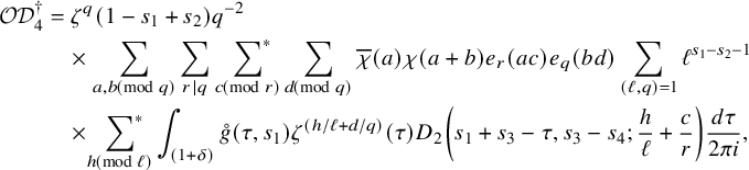 $$ \begin{align} \mathcal{OD}_{4}^{\dagger} &= \zeta^{q}(1-s_{1}+s_{2}) q^{-2} \nonumber\\&\quad \times \sum_{a, b\! \pmod{q} } \sum_{r \mid q} \ \sideset{}{^{\ast}} \sum_{c\! \pmod{r}} \sum_{d\! \pmod{q} } \overline{\chi}(a) \chi(a+b) e_{r}(ac) e_{q}(bd) \sum_{(\ell, q) = 1} \ell^{s_{1}-s_{2}-1} \notag\\ &\quad\times \sideset{}{^{\ast}} \sum_{h\! \pmod{\ell}} \int_{(1+\delta)} \mathring{g}(\tau, s_{1}) \zeta^{(h/\ell+d/q)}(\tau) D_{2} \left(s_{1}+s_{3}-\tau, s_{3}-s_{4}; \frac{h}{\ell}+\frac{c}{r} \right) \frac{d\tau}{2\pi i}, \end{align} $$
where the right-hand side of equation (3.8) is absolutely convergent in a suitable domain such as
 $$ \begin{align*} \mathcal{R}_{4, \delta} = \{(s_{1}, s_{2}, s_{3}, s_{4}) \in \mathcal{R}_{4}^{+}: \Re(s_{1}+s_{3})> 2+2\delta, \, \Re(s_{1})+1 < \Re(s_{2}), \, |s_{3}-s_{4}| < \delta \} \end{align*} $$
for an arbitrary but fixed constant $\delta $
. We then want to shift the contour to the right. In anticipation of the future application of the functional equation of the Estermann zeta function (Theorem 2.6), we define
$\delta $
. We then want to shift the contour to the right. In anticipation of the future application of the functional equation of the Estermann zeta function (Theorem 2.6), we define
 $$ \begin{align} \mathcal{E}_{4} = \left\{(s_{1}, s_{2}, s_{3}, s_{4}) \in \mathcal{B}_{4}: \Re(s_{1}+s_{3}) < \frac{B}{3}, \ \Re(s_{1}+s_{4}) < \frac{B}{3}, \ \Re(s_{1}+s_{2}+s_{3}+s_{4})> 3B \right\}. \end{align} $$
We ascertain that $\mathcal {R}_{4, \delta } \cap \mathcal {E}_{4} \ne \emptyset $
if
$\mathcal {R}_{4, \delta } \cap \mathcal {E}_{4} \ne \emptyset $
if $\delta $
is small and confine the variables
$\delta $
is small and confine the variables $(s_{1}, s_{2}, s_{3}, s_{4})$
to be in the codomain
$(s_{1}, s_{2}, s_{3}, s_{4})$
to be in the codomain $\mathcal {E}_{4}$
, and then our shift of the contour in equation (3.8) to
$\mathcal {E}_{4}$
, and then our shift of the contour in equation (3.8) to $\Re (\tau ) = B$
results in
$\Re (\tau ) = B$
results in
 $$ \begin{align} \sideset{}{^{\ast}} \sum_{h\! \pmod{\ell}} &\bigg\{\int_{(1+\delta)}-\int_{(B)} \bigg\} \mathring{g}(\tau, s_{1}) \zeta^{(h/\ell+d/q)}(\tau) D_{2} \left(s_{1}+s_{3}-\tau, s_{3}-s_{4}; \frac{h}{\ell}+\frac{c}{r} \right) \frac{d\tau}{2\pi i} \notag \\ &\qquad \ = (\ell r)^{s_{3}-s_{4}-1} \zeta(1-s_{3}+s_{4}) \mathring{g}(s_{1}+s_{3}-1, s_{1}) \sum_{n = 1}^{\infty} r_{\ell}(n) e_{q}(nd) n^{1-s_{1}-s_{3}} \notag \\ &\qquad\qquad\quad \ + (\ell r)^{s_{4}-s_{3}-1} \zeta(1+s_{3}-s_{4}) \mathring{g}(s_{1}+s_{4}-1, s_{1}) \sum_{n = 1}^{\infty} r_{\ell}(n) e_{q}(nd) n^{1-s_{1}-s_{4}}. \end{align} $$
Since the above polar terms do not contain the parameter c, one may express the sum over c in equation (3.8) as $r_{r}(a)$
, which leads one to a further simplification of them. At this stage, we notice that
$r_{r}(a)$
, which leads one to a further simplification of them. At this stage, we notice that
 $$ \begin{align} \sum_{a, b\! \pmod{q} } \overline{\chi}(a) \chi(a+b) e_{q}(ac+bd) = \tau(\chi, d) \overline{\tau(\chi, d-c)} = \overline{\chi}(d) \chi(d-c) q \end{align} $$
when $r = q$
. This evaluation will not be used as the expanded sums are more amenable. Consequently, after some rearrangements, our formula is transformed into
$r = q$
. This evaluation will not be used as the expanded sums are more amenable. Consequently, after some rearrangements, our formula is transformed into
 $$ \begin{align*} \mathcal{OD}_{4}^{\dagger} & = (\text{Polar Terms})+q^{-2} \sum_{a, b, d \pmod{q}} \sum_{r \mid q} \zeta^{r}(1-s_{1}+s_{2}) \ \sideset{}{^{\ast}} \sum_{c\! \pmod{r}} \overline{\chi}(a) \chi(a+b) e_{r}(ac) e_{q}(bd)\\ &\quad \ \times \sum_{(\ell, r) = 1} \ell^{s_{1}-s_{2}-1} \sideset{}{^{\ast}} \sum_{h\! \pmod{\ell}} \int_{(B)} \mathring{g}(\tau, s_{1}) \zeta^{(h/\ell+d/q)}(\tau) D_{2} \left(s_{1}+s_{3}-\tau, s_{3}-s_{4}; \frac{h}{\ell}+\frac{c}{r} \right) \frac{d\tau}{2\pi i}, \end{align*} $$
which is now in shape to make use of Poisson summation twice, namely Voronoĭ summation once. This is because we have $\Re (s_{1}+s_{3}-\tau ) < 0$
and
$\Re (s_{1}+s_{3}-\tau ) < 0$
and $\Re (s_{1}+s_{4}-\tau ) < 0$
; so we replace the Estermann zeta function
$\Re (s_{1}+s_{4}-\tau ) < 0$
; so we replace the Estermann zeta function $D_{2}(s_{1}+s_{3}-\tau , s_{3}-s_{4}; h/\ell +c/r)$
with the absolutely convergent series exhibited by equation (2.14).
$D_{2}(s_{1}+s_{3}-\tau , s_{3}-s_{4}; h/\ell +c/r)$
with the absolutely convergent series exhibited by equation (2.14).
3.3 Utilisation of Voronoĭ summation
This subsection aims at applying the functional equation to the sum over m and simplifying the resulting expression to a certain sum of Kloosterman sums of the form $S_{\mathfrak {ab}}(m, \pm n; c; \psi )$
. To this end, the following elementary formula is necessary: if we set
$S_{\mathfrak {ab}}(m, \pm n; c; \psi )$
. To this end, the following elementary formula is necessary: if we set $v = hr+c \ell $
with
$v = hr+c \ell $
with $(v, \ell r) = 1$
, then
$(v, \ell r) = 1$
, then
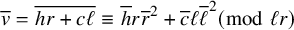 $$ \begin{align} \overline{v} = \overline{hr+c \ell} \equiv \overline{h} r \overline{r}^{2}+\overline{c} \ell \overline{\ell}^{2} \pmod{\ell r} \end{align} $$
with $h \overline {h} \equiv 1$
,
$h \overline {h} \equiv 1$
, $r \overline {r} \equiv 1 \pmod {\ell }$
and
$r \overline {r} \equiv 1 \pmod {\ell }$
and $c \overline {c} \equiv 1$
,
$c \overline {c} \equiv 1$
, $\ell \overline {\ell } \equiv 1 \pmod {r}$
. This holds under the assumption
$\ell \overline {\ell } \equiv 1 \pmod {r}$
. This holds under the assumption $(\ell , r) = 1$
. The application of Theorem 2.6 hence leads one to
$(\ell , r) = 1$
. The application of Theorem 2.6 hence leads one to
 $$ \begin{align*} \mathcal{OD}_{4}^{\dagger} &= (\text{Polar Terms})+2q^{-2} \sum_{a, b, d \pmod{q} } \sum_{r \mid q} \frac{\zeta^{r}(1-s_{1}+s_{2})}{r} \ \sideset{}{^{\ast}} \sum_{c\! \pmod{r}} \overline{\chi}(a) \chi(a+b) e_{r}(ac) e_{q}(bd)\\ & \qquad \times \sum_{(\ell, r) = 1} \ell^{s_{1}-s_{2}-2} \sideset{}{^{\ast}} \sum_{h\! \pmod{\ell}} \int_{(B)} \left(\frac{2\pi}{\ell r} \right)^{2s_{1}+s_{3}+s_{4}-2\tau-2} \zeta^{(h/\ell+d/q)}(\tau) \Gamma(1+\tau-s_{1}-s_{3})\\ & \qquad \times \Gamma(1+\tau-s_{1}-s_{4}) \bigg\{D_{2} \left(1+\tau-s_{1}-s_{3}, s_{4}-s_{3}; \frac{\overline{h} \overline{r}^{2}}{\ell} + \frac{\overline{c} \overline{\ell}^{2}}{r} \right) \cos \left(\frac{\pi(s_{3}-s_{4})}{2} \right)\\ & \qquad - D_{2} \left(1+\tau-s_{1}-s_{3}, s_{4}-s_{3}; - \frac{\overline{h} \overline{r}^{2}}{\ell}-\frac{\overline{c} \overline{\ell}^{2}}{r} \right) \cos \left(\pi \left(\frac{s_{3}+s_{4}}{2}+s_{1}-\tau \right) \right) \bigg\} \mathring{g}(\tau, s_{1}) \frac{d\tau}{2\pi i}. \end{align*} $$
We expand the integrand as the Dirichlet series once again so that the sums over c and h boil down to two Kloosterman sums, whence we are left with
 $$ \begin{align} \begin{split} \mathcal{OD}_{4}^{\dagger} &= (\text{Polar Terms})+2 (2\pi)^{s_{1}-s_{2}-1} q^{-2} \sum_{a, b, d \pmod{q} } \overline{\chi}(a) \chi(a+b) e_{q}(bd)\\ & \qquad \times \sum_{r \mid q} r^{s_{2}-s_{1}} \zeta^{r}(1-s_{1}+s_{2}) \sum_{m = 1}^{\infty} \sum_{n = 1}^{\infty} m^{(1-s_{1}-s_{2}-s_{3}-s_{4})/2} n^{(s_{1}-s_{2}+s_{3}-s_{4}-1)/2}\\ & \qquad \times e_{q}(md) \sigma_{s_{4}-s_{3}}(n) \sum_{\pm} \sum_{(\ell, r) = 1} \frac{1}{\ell} S(m, \pm n \overline{r}^{2}; \ell) S(a, \pm n \overline{\ell}^{2}; r) \Psi_{\texttt{s}}^{\pm} \left(\frac{4\pi \sqrt{mn}}{\ell r} \right), \end{split} \end{align} $$
where


The expression in equation (3.13) affirmatively answers Motohashi’s conjecture spelled out in his article [Reference Motohashi, Greaves, Harman and Huxley54] on the reciprocity formula for the second moment of Dedekind zeta functions. One ascertains that the integrand in equation (3.14) has rapid decay in $\tau $
, whereas the definition in equation (3.15) requires the properties shown in Lemma 3.2. Convention 1.10 therefore applies to control
$\tau $
, whereas the definition in equation (3.15) requires the properties shown in Lemma 3.2. Convention 1.10 therefore applies to control $\Psi _{\texttt {s}}^{-}(x)$
, which involves the opposite sign case of Kloosterman sums. This dominates the bulk of the evaluation of
$\Psi _{\texttt {s}}^{-}(x)$
, which involves the opposite sign case of Kloosterman sums. This dominates the bulk of the evaluation of $\mathcal {OD}_{4}^{\dagger }$
. We ensure this phenomenon in Proposition 3.5.
$\mathcal {OD}_{4}^{\dagger }$
. We ensure this phenomenon in Proposition 3.5.
We then manage to simplify the product of the Kloosterman sums appearing in equation (3.13). It is desirable to collapse the second Kloosterman sum to perform the separation of variables. To this end, we write $n = n_{0} n^{\prime }$
with
$n = n_{0} n^{\prime }$
with $n_{0} \mid r^{\infty }$
and
$n_{0} \mid r^{\infty }$
and $(n^{\prime }, r) = 1$
. We are in a position to use Lemma 2.3, getting
$(n^{\prime }, r) = 1$
. We are in a position to use Lemma 2.3, getting
 $$ \begin{align} S(a, \pm n \overline{\ell}^{2}; r) = \frac{1}{\varphi(r)} \sum_{\psi \pmod{r}} \psi(\ell)^{2} \overline{\psi}(\pm an^{\prime}) \tau(\psi) \tau(\psi, n_{0}), \end{align} $$
where the condition $(a, r) = 1$
was used in view of the appearance of the character
$(a, r) = 1$
was used in view of the appearance of the character $\overline {\chi }(a)$
and
$\overline {\chi }(a)$
and $\tau (\psi )$
is the Gauß sum associated to
$\tau (\psi )$
is the Gauß sum associated to $\psi $
. Dropping the primes for notational simplicity, we observe that
$\psi $
. Dropping the primes for notational simplicity, we observe that $\mathcal {OD}_{4}^{\dagger }$
equals the polar terms plus (note that the condition
$\mathcal {OD}_{4}^{\dagger }$
equals the polar terms plus (note that the condition $(n, r) = 1$
is encoded by
$(n, r) = 1$
is encoded by $\overline {\psi }(n)$
)
$\overline {\psi }(n)$
)
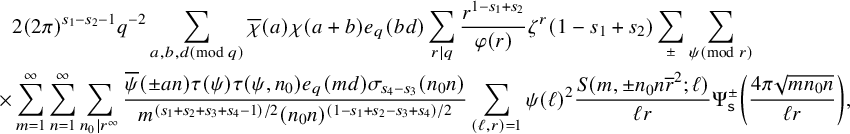 $$ \begin{align} &2 (2\pi)^{s_{1}-s_{2}-1} q^{-2} \sum_{a, b, d \pmod{q} } \overline{\chi}(a) \chi(a+b) e_{q}(bd) \sum_{r \mid q} \frac{r^{1-s_{1}+s_{2}}}{\varphi(r)} \zeta^{r}(1-s_{1}+s_{2}) \sum_{\pm} \sum_{\psi \pmod{r}} \notag\\ \times &\sum_{m = 1}^{\infty} \sum_{n = 1}^{\infty} \sum_{n_{0} \mid r^{\infty}} \frac{\overline{\psi}(\pm an) \tau(\psi) \tau(\psi, n_{0}) e_{q}(md) \sigma_{s_{4}-s_{3}}(n_{0} n)} {m^{(s_{1}+s_{2}+s_{3}+s_{4}-1)/2} (n_{0} n)^{(1-s_{1}+s_{2}-s_{3}+s_{4})/2}} \sum_{(\ell, r) = 1} \psi(\ell)^{2} \frac{S(m, \pm n_{0} n \overline{r}^{2}; \ell)}{\ell r} \Psi_{\texttt{s}}^{\pm} \left(\frac{4\pi \sqrt{mn_{0} n}}{\ell r} \right), \end{align} $$
In order to adapt the Kloosterman summation formula in its suitable form, there are two roads to proceed. The first route is to represent $S(m, \pm n_{0} n \overline {r}^{2}; \ell )$
by means of the Kloosterman sum associated to the
$S(m, \pm n_{0} n \overline {r}^{2}; \ell )$
by means of the Kloosterman sum associated to the $(\infty , 0)$
cusp-pair and apply Theorem 2.11 to the sum over
$(\infty , 0)$
cusp-pair and apply Theorem 2.11 to the sum over $\ell $
. The second is to extract the principal and quadratic character from the
$\ell $
. The second is to extract the principal and quadratic character from the $\psi $
-sum in equation (3.16) and then replace
$\psi $
-sum in equation (3.16) and then replace $S(m, \pm n_{0} n \overline {r}^{2}; \ell )$
with the twisted Kloosterman sum; namely, we make use of the formula due to Blomer–Milićević [Reference Blomer and Milićević15, black(2.2)]:
$S(m, \pm n_{0} n \overline {r}^{2}; \ell )$
with the twisted Kloosterman sum; namely, we make use of the formula due to Blomer–Milićević [Reference Blomer and Milićević15, black(2.2)]:
 $$ \begin{align} \sum_{(\ell, r) = 1} \psi(\ell)^{2} \frac{S(m, \pm n_{0} n \overline{r}^{2}; \ell)}{\ell r} \Psi_{\texttt{s}}^{\pm} \left(\frac{4\pi \sqrt{mn_{0} n}}{\ell r} \right) = \frac{\psi(m)^{2}}{\tau(\psi^{2})} \sum_{d \mid r} \mu(d) \sum_{dr \mid c} \frac{S_{\psi^{2}}(m, \pm n_{0} n; c)}{c} \Psi_{\texttt{s}}^{\pm} \left(\frac{4\pi \sqrt{mn_{0} n}}{c} \right), \end{align} $$
where $S_{\psi }(m, n; c)$
is defined in equation (2.17) and
$S_{\psi }(m, n; c)$
is defined in equation (2.17) and $\psi $
denotes a primitive nonquadratic character modulo r so that
$\psi $
denotes a primitive nonquadratic character modulo r so that $\psi ^{2}$
is primitive. This is where the assumption of q being prime is used, since the square of a nonquadratic character is not necessarily primitive (see Remark 3.4). Nevertheless, one may remove this assumption via the use of an extended form of equation (3.18). Note that equation (3.18) is only available when
$\psi ^{2}$
is primitive. This is where the assumption of q being prime is used, since the square of a nonquadratic character is not necessarily primitive (see Remark 3.4). Nevertheless, one may remove this assumption via the use of an extended form of equation (3.18). Note that equation (3.18) is only available when $(m, r) = 1$
. As shall be seen later, the Dirichlet character
$(m, r) = 1$
. As shall be seen later, the Dirichlet character $\overline {\psi }(m)$
arises if we calculate the character sums in equation (3.17). We need to take the second route for technical simplicity. The off-diagonal term
$\overline {\psi }(m)$
arises if we calculate the character sums in equation (3.17). We need to take the second route for technical simplicity. The off-diagonal term $\mathcal {OD}_{4}^{\dagger }$
is thus equal to the polar terms plus
$\mathcal {OD}_{4}^{\dagger }$
is thus equal to the polar terms plus
 $$ \begin{align*} &2 (2\pi)^{s_{1}-s_{2}-1} q^{-2} \sum_{a, b, c\! \pmod{q} } \overline{\chi}(a) \chi(a+b) e_{q}(bc) \sum_{r \mid q} \frac{r^{1-s_{1}+s_{2}}}{\varphi(r)} \zeta^{r}(1-s_{1}+s_{2})\\ &\qquad\quad \times \sum_{\pm} \Bigg\{\ \sideset{}{^{\#}} \sum_{\psi \pmod{r}} \frac{\overline{\psi}(\pm a) \tau(\psi)}{\tau(\psi^{2})} \sum_{m = 1}^{\infty} \sum_{n = 1}^{\infty} \sum_{n_{0} \mid r^{\infty}} \frac{\psi(m)^{2} \overline{\psi}(n) \tau(\psi, n_{0}) e_{q}(mc) \sigma_{s_{4}-s_{3}}(n_{0} n)} {m^{(s_{1}+s_{2}+s_{3}+s_{4}-1)/2} (n_{0} n)^{(1-s_{1}+s_{2}-s_{3}+s_{4})/2}}\\ &\qquad\qquad\qquad\qquad\qquad\qquad\qquad\qquad \ \times \sum_{d \mid r} \mu(d) \sum_{dr \mid c} \frac{S_{\psi^{2}}(m, \pm n_{0} n; c)}{c} \Psi_{\texttt{s}}^{\pm} \left(\frac{4\pi \sqrt{mn_{0} n}}{c} \right)+\mathcal{R} \Bigg\}, \end{align*} $$
where $\#$
on the
$\#$
on the $\psi $
-sum means that the sum ranges over all primitive nonquadratic characters modulo r and
$\psi $
-sum means that the sum ranges over all primitive nonquadratic characters modulo r and $\mathcal {R}$
serves as the remainder term
$\mathcal {R}$
serves as the remainder term
 $$ \begin{align*} \mathcal{R} = \sideset{}{^{\flat}} \sum_{\psi \pmod{r}} \sum_{m = 1}^{\infty} \sum_{n = 1}^{\infty} \sum_{n_{0} \mid r^{\infty}} &\frac{\psi(\pm na) \tau(\psi) \tau(\psi, n_{0}) e_{q}(mc) \sigma_{s_{4}-s_{3}}(n_{0} n)} {m^{(s_{1}+s_{2}+s_{3}+s_{4}-1)/2} (n_{0} n)^{(1-s_{1}+s_{2}-s_{3}+s_{4})/2}}\\ &\qquad\qquad\qquad\qquad\qquad\quad \ \times \sum_{(\ell, r) = 1} \frac{S(m, \pm n_{0} n \overline{r}^{2}; \ell)}{\ell r} \Psi_{\texttt{s}}^{\pm} \left(\frac{4\pi \sqrt{mn_{0} n}}{\ell r} \right). \end{align*} $$
Here $\flat $
on the
$\flat $
on the $\psi $
-sum means that the sum ranges over the principal and the quadratic character modulo r. Since it follows that
$\psi $
-sum means that the sum ranges over the principal and the quadratic character modulo r. Since it follows that $\tau (\psi , n_{0}) = \overline {\psi }(n_{0}) \tau (\psi )$
in the case where
$\tau (\psi , n_{0}) = \overline {\psi }(n_{0}) \tau (\psi )$
in the case where $\psi $
is a primitive nonquadratic character, we can take
$\psi $
is a primitive nonquadratic character, we can take $n_{0} = 1$
due to the condition
$n_{0} = 1$
due to the condition $n_{0} \mid r^{\infty }$
. In order to reduce the character sums over
$n_{0} \mid r^{\infty }$
. In order to reduce the character sums over $a, b, c$
, we start with simplifying the c-sum, obtaining
$a, b, c$
, we start with simplifying the c-sum, obtaining
 $$ \begin{align*} \sum_{a, b, c\! \pmod{q} } \overline{\chi}(a) \overline{\psi}(a) \chi(a+b) e_{q}((b+m)c) = \psi(-1) q \sum_{a\! \pmod{q} } \overline{\chi}(a) \overline{\psi}(a) \chi(a+m). \end{align*} $$
When $\chi \psi $
is primitive, one can set
$\chi \psi $
is primitive, one can set $\psi _{1} = \overline {\chi \psi }$
and
$\psi _{1} = \overline {\chi \psi }$
and $\psi _{2} = \chi $
in Lemma 2.2. To be more general, we deduce
$\psi _{2} = \chi $
in Lemma 2.2. To be more general, we deduce
 $$ \begin{align*} \sum_{a\! \pmod{q} } \overline{\chi}(a) \overline{\psi}(a) \chi(a+m) = \frac{1}{\tau(\overline{\chi})} \sum_{a, b\! \pmod{q} } \overline{\chi}(ab) \overline{\psi}(a) e \left(\frac{(a+m)b}{q} \right) = \frac{\tau(\overline{\chi \psi}) \tau(\psi, m)}{\tau(\overline{\chi})}. \end{align*} $$
Since the sum over primitive nonquadratic characters is empty when $r = 1$
, we have proven the following:
$r = 1$
, we have proven the following:
Proposition 3.3. For any primitive Dirichlet character $\chi $
modulo a prime q, the function
$\chi $
modulo a prime q, the function $\mathcal {OD}_{4}^{\dagger }$
can be meromorphically continued to the domain
$\mathcal {OD}_{4}^{\dagger }$
can be meromorphically continued to the domain $\mathcal {E}_{4}$
, and there we have
$\mathcal {E}_{4}$
, and there we have
 $$ \begin{align*} \mathcal{OD}_{4}^{\dagger} = \mathcal{P}+\sum_{\pm} \left\{\mathcal{J}_{\pm}+\mathcal{E}_{\pm} \right\}. \end{align*} $$
Here for the multiplicative function

we set
 $$ \begin{align*} \mathcal{P} &= A_{q}(s_{1}, s_{2}, s_{3}, s_{4}) \mathring{g}(s_{1}+s_{3}-1, s_{1}) \frac{\zeta^{q}(1-s_{1}+s_{2}) \zeta^{q}(1-s_{3}+s_{4}) \zeta(s_{2}+s_{4}) \zeta(s_{1}+s_{3}-1)}{\zeta^{q}(s_{2}+s_{4}-s_{1}-s_{3}+2)}\\ &\quad + A_{q}(s_{1}, s_{2}, s_{4}, s_{3}) \mathring{g}(s_{1}+s_{4}-1, s_{1}) \frac{\zeta^{q}(1-s_{1}+s_{2}) \zeta^{q}(1+s_{3}-s_{4}) \zeta(s_{2}+s_{3}) \zeta(s_{1}+s_{4}-1)}{\zeta^{q}(s_{2}+s_{3}-s_{1}-s_{4}+2)}, \end{align*} $$
 $$ \begin{align} \mathcal{J}_{\pm} &= \frac{2\zeta^{q}(1-s_{1}+s_{2})}{\tau(\overline{\chi}) \varphi(q) q} \left(\frac{2\pi}{q} \right)^{s_{1}-s_{2}-1} \ \sideset{}{^{\#}} \sum_{\psi \pmod{q} } \psi(\mp 1) \tau(\psi) \tau(\overline{\chi \psi}) J(\psi, \psi) \sum_{d \mid q} \mu(d) \notag\\ &\quad \times \sum_{m = 1}^{\infty} \sum_{n = 1}^{\infty} \psi(m) \overline{\psi}(n) m^{(1-s_{1}-s_{2}-s_{3}-s_{4})/2} n^{(s_{1}-s_{2}+s_{3}-s_{4}-1)/2} \sigma_{s_{4}-s_{3}}(n) \, \mathcal{O}_{\infty \infty}^{dq}(m, \pm n; \Psi_{\texttt{s}}^{\pm}; \psi^{2}), \end{align} $$
 $$ \begin{align} &\mathcal{E}_{\pm} = \frac{2(2\pi)^{s_{1}-s_{2}-1}}{\tau(\overline{\chi}) q} \sum_{r \mid q} \frac{r^{1-s_{1}+s_{2}}}{\varphi(r)} \zeta^{r}(1-s_{1}+s_{2}) \ \sideset{}{^{\flat}} \sum_{\psi \pmod{r}} \psi(\mp 1) \tau(\psi) \tau(\overline{\chi} \psi) \sum_{m = 1}^{\infty} \sum_{n = 1}^{\infty} \sum_{n_{0} \mid r^{\infty}} \psi(n) \notag\\ \times\, &\tau(\psi, m) \tau(\psi, n_{0}) m^{(1-s_{1}-s_{2}-s_{3}-s_{4})/2} (n_{0} n)^{(s_{1}-s_{2}+s_{3}-s_{4}-1)/2} \sigma_{s_{4}-s_{3}}(n_{0} n) \, \mathcal{O}_{\infty 0}^{r^{2}}(m, \pm n_{0} n; \Psi_{\texttt{s}}^{\pm}; \psi_{0}), \end{align} $$
where $\mathcal {O}_{\mathfrak {ab}}^{q}(m, \pm n; \Psi _{\texttt {s}}^{\pm }; \psi )$
is defined in Theorem 2.11.
$\mathcal {O}_{\mathfrak {ab}}^{q}(m, \pm n; \Psi _{\texttt {s}}^{\pm }; \psi )$
is defined in Theorem 2.11.
Remark 3.4. The square of a primitive nonquadratic Dirichlet character of composite modulus having at least two prime factors is not primitive. For instance, one may choose a primitive quadratic character $\psi _{1}$
(respectively, nonquadratic character
$\psi _{1}$
(respectively, nonquadratic character $\psi _{2}$
) modulo
$\psi _{2}$
) modulo $3$
(respectively, modulo
$3$
(respectively, modulo $5$
) and combine them to obtain a character
$5$
) and combine them to obtain a character $\psi _{1} \psi _{2}$
modulo
$\psi _{1} \psi _{2}$
modulo $15$
as follows:
$15$
as follows:
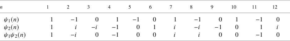
The multiplication of Dirichlet characters of different moduli gives a Dirichlet character modulo a least common multiple. We define $\psi = \psi _{1} \psi _{2}$
, which is nonquadratic since it involves i and
$\psi = \psi _{1} \psi _{2}$
, which is nonquadratic since it involves i and $-i$
as values and is primitive since it cannot be induced from a Dirichlet character modulo
$-i$
as values and is primitive since it cannot be induced from a Dirichlet character modulo $1$
,
$1$
, $3$
, or
$3$
, or $5$
. However,
$5$
. However, $\psi ^{2} = \psi _{1}^{2} \psi _{2}^{2}$
is induced from a quadratic character modulo 5. This is why we assume that q is prime in this work.
$\psi ^{2} = \psi _{1}^{2} \psi _{2}^{2}$
is induced from a quadratic character modulo 5. This is why we assume that q is prime in this work.
Proof. For the first assertion, one can check that both series in equations (3.19) and (3.20) converge absolutely and uniformly in $\mathcal {E}_{4}$
, proving the meromorphic continuation of
$\mathcal {E}_{4}$
, proving the meromorphic continuation of $\mathcal {OD}_{4}^{\dagger }$
to
$\mathcal {OD}_{4}^{\dagger }$
to $\mathbb {C}^{4}$
. A remarkable point is that we only need the Weil bound in equation (2.5) for Kloosterman sums. For the second assertion, it suffices to compute the polar terms. We decompose
$\mathbb {C}^{4}$
. A remarkable point is that we only need the Weil bound in equation (2.5) for Kloosterman sums. For the second assertion, it suffices to compute the polar terms. We decompose $\mathcal {P} = \mathcal {P}_{1}+\mathcal {P}_{2}$
, where
$\mathcal {P} = \mathcal {P}_{1}+\mathcal {P}_{2}$
, where $\mathcal {P}_{1}$
(respectively,
$\mathcal {P}_{1}$
(respectively, $\mathcal {P}_{2}$
) stems from the first term (respectively, second term) on the right-hand side of equation (3.10). First of all, we remark that the polar contribution
$\mathcal {P}_{2}$
) stems from the first term (respectively, second term) on the right-hand side of equation (3.10). First of all, we remark that the polar contribution $\mathcal {P}$
is expressed as
$\mathcal {P}$
is expressed as
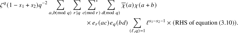 $$ \begin{align*} \zeta^{q}(1-s_{1}+s_{2}) q^{-2} &\sum_{a, b\! \pmod{q} } \sum_{r \mid q} \ \sideset{}{^{\ast}} \sum_{c\! \pmod{r}} \sum_{d\! \pmod{q} } \overline{\chi}(a) \chi(a+b)\\ &\qquad\qquad\qquad \times e_{r}(ac) e_{q}(bd) \sum_{(\ell, q) = 1} \ell^{s_{1}-s_{2}-1} \times (\text{RHS of equation (3.10)}). \end{align*} $$
In the following lines, we deal with $\mathcal {P}_{1}$
. The sum over
$\mathcal {P}_{1}$
. The sum over $\ell $
is reduced to
$\ell $
is reduced to
 $$ \begin{align*} \sum_{(\ell, q) = 1} \ell^{s_{1}-s_{2}+s_{3}-s_{4}-2} r_{\ell}(n) = \zeta^{q}(s_{2}+s_{4}-s_{1}-s_{3}+2)^{-1} \sigma_{s_{1}-s_{2}+s_{3}-s_{4}-1}(n). \end{align*} $$
We are in a position to manipulate the exponential sums. The sum over d gives rise to
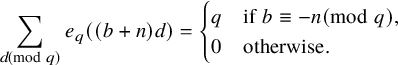 $$ \begin{align*} \sum_{d\! \pmod{q} } e_{q}((b+n)d) = \begin{cases} q & \text{if } b \equiv -n \pmod{q} ,\\ 0 & \text{otherwise}. \end{cases} \end{align*} $$
This renders
 $$ \begin{align*} \sum_{a\! \pmod{q} } \overline{\chi}(a) \chi(a-n) r_{r}(a) = \frac{\mu(r)}{\tau(\overline{\chi})} \sum_{a, b\! \pmod{q} } \overline{\chi}(ab) e_{q}((a+n)b) = \mu(r) r_{q}(n). \end{align*} $$
In this manner, the sums over $a, b, c, d$
can be eliminated. In general, the sum over r turns into
$a, b, c, d$
can be eliminated. In general, the sum over r turns into
 $$ \begin{align*} \sum_{r \mid q} \mu(r) r^{s_{3}-s_{4}-1} = \prod_{p \mid q} \left(1-\frac{1}{p^{1-s_{3}+s_{4}}} \right), \end{align*} $$
which yields $\zeta ^{q}(1-s_{3}+s_{4})$
when combined with
$\zeta ^{q}(1-s_{3}+s_{4})$
when combined with $\zeta (1-s_{3}+s_{4})$
. We hence obtain
$\zeta (1-s_{3}+s_{4})$
. We hence obtain
 $$ \begin{align*} \mathcal{P}_{1} = \frac{\mathring{g}(s_{1}+s_{3}-1, s_{1})}{q} \frac{\zeta^{q}(1-s_{1}+s_{2}) \zeta^{q}(1-s_{3}+s_{4})}{\zeta^{q}(s_{2}+s_{4}-s_{1}-s_{3}+2)} \sum_{n = 1}^{\infty} \frac{\sigma_{s_{1}-s_{2}+s_{3}-s_{4}-1}(n) r_{q}(n)}{n^{s_{1}+s_{3}-1}}. \end{align*} $$
Having mentioned this expression, we need to calculate the the sum over n via Lemma 2.5, getting
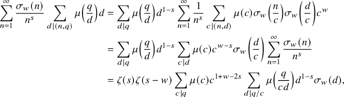 $$ \begin{align*} \sum_{n = 1}^{\infty} \frac{\sigma_{w}(n)}{n^{s}} \sum_{d \mid (n, q)} \mu \left(\frac{q}{d} \right) d & = \sum_{d \mid q} \mu \left(\frac{q}{d} \right) d^{1-s} \sum_{n = 1}^{\infty} \frac{1}{n^{s}} \sum_{c \mid (n, d)} \mu(c) \sigma_{w} \left(\frac{n}{c} \right) \sigma_{w} \left(\frac{d}{c} \right) c^{w}\\ & = \sum_{d \mid q} \mu \left(\frac{q}{d} \right) d^{1-s} \sum_{c \mid d} \mu(c) c^{w-s} {\sigma_{w} \left(\frac{d}{c} \right)} \sum_{n = 1}^{\infty} \frac{\sigma_{w}(n)}{n^{s}}\\ & = \zeta(s) \zeta(s-w) \sum_{c \mid q} \mu(c) c^{1+w-2s} \sum_{d \mid q/c} \mu \left(\frac{q}{cd} \right) d^{1-s} \sigma_{w}(d), \end{align*} $$
where $s = s_{1}+s_{3}-1$
and
$s = s_{1}+s_{3}-1$
and $w = s_{1}-s_{2}+s_{3}-s_{4}-1$
. Notice that the right-hand side can be written as a Dirichlet convolution of multiplicative functions. Recall that the Dirichlet convolution is defined as
$w = s_{1}-s_{2}+s_{3}-s_{4}-1$
. Notice that the right-hand side can be written as a Dirichlet convolution of multiplicative functions. Recall that the Dirichlet convolution is defined as
 $$ \begin{align*} (f \ast g)(m) = \sum_{d \mid m} f(d) g \left(\frac{m}{d} \right), \end{align*} $$
which is an associative and commutative binary operation on arithmetic functions. If f and g are assumed to be multiplicative, so is $f \ast g$
. Setting
$f \ast g$
. Setting
![]() and
and
![]() , we have that
, we have that
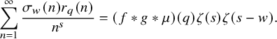 $$ \begin{align*} \sum_{n = 1}^{\infty} \frac{\sigma_{w}(n) r_{q}(n)}{n^{s}} = (f \ast g \ast \mu)(q) \zeta(s) \zeta(s-w). \end{align*} $$
This finishes the proof of Proposition 3.3.
3.4 Utilisation of the Kuznetsov formula
We now apply the automorphic machinery in Section 2 to our sums of Kloosterman sums along with a careful analysis of integrals involving various Bessel functions. We focus on the treatment of $\mathcal {O}_{\infty \mathfrak {b}}^{dq}(m, \pm n; \Psi _{\texttt {s}}^{\pm }; \psi )$
with
$\mathcal {O}_{\infty \mathfrak {b}}^{dq}(m, \pm n; \Psi _{\texttt {s}}^{\pm }; \psi )$
with $\mathfrak {b} = \infty , 0$
in an across-the-board manner and implement the substitutions at the end to calculate
$\mathfrak {b} = \infty , 0$
in an across-the-board manner and implement the substitutions at the end to calculate $\mathcal {J}_{\pm }$
and
$\mathcal {J}_{\pm }$
and $\mathcal {E}_{\pm }$
. The three-time differentiability and the decay condition at
$\mathcal {E}_{\pm }$
. The three-time differentiability and the decay condition at $x = 0$
in Theorem 2.11 are fulfilled. Moreover, the decay condition at infinity follows by shifting the contours
$x = 0$
in Theorem 2.11 are fulfilled. Moreover, the decay condition at infinity follows by shifting the contours $\Re (s) = B$
in equations (3.14) and (3.15) to the right and then applying Lemma 3.2. We forthwith derive the spectral decomposition
$\Re (s) = B$
in equations (3.14) and (3.15) to the right and then applying Lemma 3.2. We forthwith derive the spectral decomposition
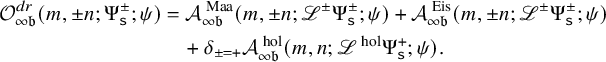
Complying with Motohashi’s book [Reference Motohashi55], one observes how the case of the plus sign contributes. In order to reduce the integral transform $\mathscr {L}^{+}$
, we consider, in the light of the definition in equation (3.14), the double integral
$\mathscr {L}^{+}$
, we consider, in the light of the definition in equation (3.14), the double integral
 $$ \begin{align} \int_{0}^{\infty} J_{2it}(\eta) \int_{(B)} \Gamma(1+\tau-s_{1}-s_{3}) \Gamma(1+\tau-s_{1}-s_{4}) \left(\frac{\eta}{2} \right)^{s_{1}+s_{2}+s_{3}+s_{4}-2-2\tau} \mathring{g}(\tau, s_{1}) d\tau d\eta, \end{align} $$
where $\mathring {g}$
is the Mellin transform in equation (3.5). This double integral is holomorphic in the domain
$\mathring {g}$
is the Mellin transform in equation (3.5). This double integral is holomorphic in the domain
 $$ \begin{align} \left\{(s_{1}, s_{2}, s_{3}, s_{4}) \in \mathbb{C}^{4}: \begin{array}{l} \Re(s_{1}+s_{3}) < 1+B, \, \Re(s_{1}+s_{4}) < 1+B,\\ 1+2B < \Re(s_{1}+s_{2}+s_{3}+s_{4}) < 3/2+2A \end{array} \right\}, \end{align} $$
which contains $\mathcal {E}_{4}$
defined in equation (3.9) and
$\mathcal {E}_{4}$
defined in equation (3.9) and $A> B$
is the same as in Convention 1.10. To prove this fact, we divide equation (3.22) into two parts according as
$A> B$
is the same as in Convention 1.10. To prove this fact, we divide equation (3.22) into two parts according as $0 \leqslant \eta < 1$
and
$0 \leqslant \eta < 1$
and $\eta \geqslant 1$
and note that
$\eta \geqslant 1$
and note that
 $$ \begin{align*} J_{2it}(\eta) \ll \begin{cases} 1 & \text{as } \eta \to 0,\\ \eta^{-1/2} & \text{as } \eta \to \infty, \end{cases} \end{align*} $$
where we implicitly assumed that t is real. The first part is clearly holomorphic in the domain of equation (3.23). To estimate the second part, we move the contour in the $\tau $
-integral to
$\tau $
-integral to $\Re (\tau ) = A$
. We would like to consider the subdomain of equation (3.23) where we have
$\Re (\tau ) = A$
. We would like to consider the subdomain of equation (3.23) where we have $1+2B < \Re (s_{1}+s_{2}+s_{3}+s_{4}) < 3/2+2B$
. There the integral in equation (3.22) is absolutely and uniformly convergent in view of the power series expansion of the J-Bessel function
$1+2B < \Re (s_{1}+s_{2}+s_{3}+s_{4}) < 3/2+2B$
. There the integral in equation (3.22) is absolutely and uniformly convergent in view of the power series expansion of the J-Bessel function
 $$ \begin{align*} J_{\nu}(y) &= \sqrt{\frac{2}{\pi y}} \bigg\{\cos \left(y-\frac{\pi}{2} \left(\nu+\frac{1}{2} \right) \right) \sum_{m = 0}^{M} (-1)^{m} \begin{pmatrix} \nu-1/2 \\ 2m \end{pmatrix} \frac{\Gamma(\nu+1/2+2m)}{\Gamma(\nu+1/2)(2y)^{2m}}\\ & \quad - \sin \left(y-\frac{\pi}{2} \left(\nu+\frac{1}{2} \right) \right) \sum_{m = 0}^{M} (-1)^{m} \begin{pmatrix} \nu-1/2 \\ 2m+1 \end{pmatrix} \frac{\Gamma(\nu+3/2+2m)}{\Gamma(\nu+1/2)(2y)^{2m+1}} \bigg\}+\mathrm{O}(y^{-\Re(\nu)-3/2-2M}), \end{align*} $$
provided $\Re (\nu )> -2M-3/2$
. Hence, the double integral in equation (3.22) equals
$\Re (\nu )> -2M-3/2$
. Hence, the double integral in equation (3.22) equals
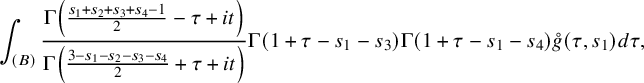 $$ \begin{align} \int_{(B)} \frac{\Gamma \left(\frac{s_{1}+s_{2}+s_{3}+s_{4}-1}{2}-\tau+it \right)} {\Gamma \left(\frac{3-s_{1}-s_{2}-s_{3}-s_{4}}{2}+\tau+it \right)} \Gamma(1+\tau-s_{1}-s_{3}) \Gamma(1+\tau-s_{1}-s_{4}) \mathring{g}(\tau, s_{1}) d\tau, \end{align} $$
where we have used the formula
 $$ \begin{align*} \int_{0}^{\infty} J_{\nu}(\eta) \left(\frac{\eta}{2} \right)^{-\mu} d\eta = \Gamma \left(\frac{1+\nu-\mu}{2} \right) \Gamma \left(\frac{1+\nu+\mu}{2} \right)^{-1} \end{align*} $$
valid for $1/2 < \Re (\mu ) < 1+\Re (\nu )$
. Since the integral in equation (3.24) is regular in equation (3.23), the analytic continuation implies that the double integral in equation (3.22) is equal to equation (3.24) throughout the domain of equation (3.23) or
$1/2 < \Re (\mu ) < 1+\Re (\nu )$
. Since the integral in equation (3.24) is regular in equation (3.23), the analytic continuation implies that the double integral in equation (3.22) is equal to equation (3.24) throughout the domain of equation (3.23) or $\mathcal {E}_{4}$
. At this stage, we note that the following identities hold:
$\mathcal {E}_{4}$
. At this stage, we note that the following identities hold:
 $$ \begin{align*} \frac{\Gamma(a-\tau+it)}{\Gamma(1-a+\tau+it)}-\frac{\Gamma(a-\tau-it)}{\Gamma(1-a+\tau-it)} & = \frac{2}{\pi i} \sinh(\pi t) \cos(\pi(a-\tau)) \Gamma(a-\tau+it) \Gamma(a-\tau-it),\\ \frac{\Gamma(a-\tau+it)}{\Gamma(1-a+\tau+it)}+\frac{\Gamma(a-\tau-it)}{\Gamma(1-a+\tau-it)} & = \frac{2}{\pi} \cosh(\pi t) \sin(\pi(a-\tau)) \Gamma(a-\tau+it) \Gamma(a-\tau-it). \end{align*} $$
which follows from the functional equation $\Gamma (s) \Gamma (1-s) = \pi /\sin (\pi s)$
. Substituting
$\Gamma (s) \Gamma (1-s) = \pi /\sin (\pi s)$
. Substituting $a = (s_{1}+s_{2}+s_{3}+s_{4}-1)/2$
, we obtain after some rearrangement thatFootnote
5
$a = (s_{1}+s_{2}+s_{3}+s_{4}-1)/2$
, we obtain after some rearrangement thatFootnote
5
 $$ \begin{align*} \mathscr{L}^{+} \Psi_{\texttt{s}}^{+}(t) &= (it \coth(\pi t))^{\kappa} \cos \left(\frac{\pi(s_{3}-s_{4})}{2} \right) \int_{(B)} \sin \left(\frac{\pi(s_{1}+s_{2}+s_{3}+s_{4}-\kappa-2\tau)}{2} \right)\\ & \qquad \times \Gamma \left(\frac{s_{1}+s_{2}+s_{3}+s_{4}-1}{2}+it-\tau \right) \Gamma \left(\frac{s_{1}+s_{2}+s_{3}+s_{4}-1}{2}-it-\tau \right)\\ & \qquad \times \Gamma(1+\tau-s_{1}-s_{3}) \Gamma(1+\tau-s_{1}-s_{4}) \mathring{g}(\tau, s_{1}) \frac{d\tau}{\pi i}. \end{align*} $$
In a similar fashion, the holomorphic contribution turns into
 $$ \begin{align*} \mathscr{L}^{\;\text{hol}} \Psi_{\texttt{s}}^{+}(k) &= i^{k-1} \cos \left(\frac{\pi(s_{3}-s_{4})}{2} \right) \int_{(B)} \frac{\Gamma \left(\frac{k+s_{1}+s_{2}+s_{3}+s_{4}-2}{2}-\tau \right)} {\Gamma \left(\frac{k+2-s_{1}-s_{2}-s_{3}-s_{4}}{2}+\tau \right)}\\ &\quad \times \Gamma(1+\tau-s_{1}-s_{3}) \Gamma(1+\tau-s_{1}-s_{4}) \mathring{g}(\tau, s_{1}) d\tau. \end{align*} $$
To proceed, we focus on the context of the minus sign. In this case, the bound shown in Lemma 3.2 plays a crucial rôle. By definition, the integral transform in question is written as
 $$ \begin{align*} \mathscr{L}^{-} \Psi_{\texttt{s}}^{-}(t) = 8i^{-\kappa} \cosh(\pi t) \int_{0}^{\infty} \Psi_{\texttt{s}}^{-}(\eta) K_{2it}(\eta) \frac{d\eta}{\eta}. \end{align*} $$
Inserting equation (3.15), we obtain an absolutely convergent integral, for we have the growth condition
 $$ \begin{align*} K_{2it}(\eta) \ll \begin{cases} |\log \eta| & \text{as } \eta \to 0,\\ \exp(-\eta) & \text{as } \eta \to \infty. \end{cases} \end{align*} $$
Substituting Heaviside’s integral formula
 $$ \begin{align} \int_{0}^{\infty} K_{2v}(\eta) \left(\frac{\eta}{2} \right)^{2s-1} d\eta = \frac{\Gamma(s+v) \Gamma(s-v)}{2} \quad \text{for} \quad \Re(s)> |\Re(v)|, \end{align} $$
we are left with the expression
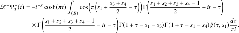 $$ \begin{align*} \mathscr{L}^{-} \Psi_{\texttt{s}}^{-}(t) &= -i^{-\kappa} \cosh(\pi t) \int_{(B)} \cos \left(\pi \left(s_{1}+\frac{s_{3}+s_{4}}{2}-\tau \right) \right) \Gamma \left(\frac{s_{1}+s_{2}+s_{3}+s_{4}-1}{2}+it-\tau \right)\\ &\quad \times \Gamma \left(\frac{s_{1}+s_{2}+s_{3}+s_{4}-1}{2}-it-\tau \right) \Gamma(1+\tau-s_{1}-s_{3}) \Gamma(1+\tau-s_{1}-s_{4}) \mathring{g}(\tau, s_{1}) \frac{d\tau}{\pi i}. \end{align*} $$
In anticipation of future simplifications of $\mathscr {L}^{\pm } \Psi _{\texttt {s}}^{\pm }(t)$
, we define the the integral transforms
$\mathscr {L}^{\pm } \Psi _{\texttt {s}}^{\pm }(t)$
, we define the the integral transforms

and

along with the original integral transform

Here the contour in the formula for $\Phi _{\texttt {s}}^{+}(\xi )$
is curved to ensure that the poles of the first two gamma factors in the integrand lie to the right of the contour and those of the other factors are on the left of the contour. In addition, the variables
$\Phi _{\texttt {s}}^{+}(\xi )$
is curved to ensure that the poles of the first two gamma factors in the integrand lie to the right of the contour and those of the other factors are on the left of the contour. In addition, the variables $\xi , s_{1}, s_{2}, s_{3}, s_{4}$
are assumed to be such that the path can be drawn. The contour in the definition of
$\xi , s_{1}, s_{2}, s_{3}, s_{4}$
are assumed to be such that the path can be drawn. The contour in the definition of $\Phi _{\texttt {s}}^{-}(\xi )$
is chosen in just the same way. On the other hand, the contour in
$\Phi _{\texttt {s}}^{-}(\xi )$
is chosen in just the same way. On the other hand, the contour in $\Xi $
separates the poles of
$\Xi $
separates the poles of $\Gamma (\xi +(s_{1}+s_{2}+s_{3}+s_{4}-1)/2-\tau )$
and those of
$\Gamma (\xi +(s_{1}+s_{2}+s_{3}+s_{4}-1)/2-\tau )$
and those of $\Gamma (1+\tau -s_{1}-s_{3}) \Gamma (1+\tau -s_{1}-s_{4}) \mathring {g}(\tau , s_{1})$
to the left and the right of the contour. An explicit formulation of the integral transforms can be executed:
$\Gamma (1+\tau -s_{1}-s_{3}) \Gamma (1+\tau -s_{1}-s_{4}) \mathring {g}(\tau , s_{1})$
to the left and the right of the contour. An explicit formulation of the integral transforms can be executed:
Proposition 3.5. With the notation above, we have that
 $$ \begin{align*} \Phi_{\texttt{s}}^{+}(\xi) &= -(-i\xi)^{\kappa} \frac{(2\pi)^{s_{1}-s_{2}}}{2\sin(\pi \xi)} \cos \left(\frac{\pi(s_{3}-s_{4})}{2} \right) \Big\{\Xi_{\texttt{s}}(\xi)-(-1)^{\kappa} \Xi_{\texttt{s}}(-\xi) \Big\},\\ \Phi_{\texttt{s}}^{-}(\xi) &= i^{-\kappa} \frac{(2\pi)^{s_{1}-s_{2}}}{2\sin(\pi \xi)} \left\{\sin \left(\pi \left(\frac{s_{2}-s_{1}}{2}+\xi \right) \right) \Xi_{\texttt{s}}(\xi) - \sin \left(\pi \left(\frac{s_{2}-s_{1}}{2}-\xi \right) \right) \Xi_{\texttt{s}}(-\xi) \right\}, \end{align*} $$
provided the left-hand sides are well-defined. We also have for real t and $\texttt {s} = (s_{1}, s_{2}, s_{3}, s_{4}) \in \mathcal {E}_{4}$
that
$\texttt {s} = (s_{1}, s_{2}, s_{3}, s_{4}) \in \mathcal {E}_{4}$
that
 $$ \begin{align*} \mathscr{L}^{+} \Psi_{\texttt{s}}^{+}(t) = (2\pi)^{1-s_{1}+s_{2}} \Phi_{\texttt{s}}^{+}(it),\\ \mathscr{L}^{-} \Psi_{\texttt{s}}^{-}(t) = (2\pi)^{1-s_{1}+s_{2}} \Phi_{\texttt{s}}^{-}(it). \end{align*} $$
For integral $k \equiv \kappa \pmod {2}$
and
$k \equiv \kappa \pmod {2}$
and $(s_{1}, s_{2}, s_{3}, s_{4}) \in \mathcal {E}_{4}$
, we have that
$(s_{1}, s_{2}, s_{3}, s_{4}) \in \mathcal {E}_{4}$
, we have that
 $$ \begin{align*} \mathscr{L}^{\;\mathrm{hol}} \Psi_{\texttt{s}}^{+}(k) = 2\pi i^{k} \cos \left(\frac{\pi(s_{3}-s_{4})}{2} \right) \Xi_{\texttt{s}} \left(\frac{k-1}{2} \right). \end{align*} $$
Proof. The proof proceeds as in [Reference Motohashi55, Lemma 4.4] mutatis mutandis.
Remark 3.6. From Proposition 3.3, we observe that all Dirichlet characters in question are of the form $\psi ^{2}$
. It therefore suffices to treat the case of
$\psi ^{2}$
. It therefore suffices to treat the case of $\kappa (\psi ^{2}) = 0$
in what follows. This should not cause any problem, although we have suppressed the dependence on
$\kappa (\psi ^{2}) = 0$
in what follows. This should not cause any problem, although we have suppressed the dependence on $\psi $
from the functions
$\psi $
from the functions $\Phi _{\texttt {s}}^{\pm }(\xi )$
and
$\Phi _{\texttt {s}}^{\pm }(\xi )$
and $\Xi _{\texttt {s}}(\xi )$
.
$\Xi _{\texttt {s}}(\xi )$
.
3.5 Deduction of the cubic moment side
We devote this subsection to the derivation of the cubic moment side. The absolute convergence that we would like to check is apparent as far as the double summation over the variables $m, n$
is concerned, since we have the bound in equation (2.22) on the Hecke eigenvalues and
$m, n$
is concerned, since we have the bound in equation (2.22) on the Hecke eigenvalues and $\texttt {s} = (s_{1}, s_{2}, s_{3}, s_{4}) \in \mathcal {E}_{4}$
. Hence, the chief issue is reduced to bounding
$\texttt {s} = (s_{1}, s_{2}, s_{3}, s_{4}) \in \mathcal {E}_{4}$
. Hence, the chief issue is reduced to bounding $\mathscr {L}^{\pm } \Psi _{\texttt {s}}^{\pm }$
, and then Proposition 3.5 reduces our task to the analysis of the function
$\mathscr {L}^{\pm } \Psi _{\texttt {s}}^{\pm }$
, and then Proposition 3.5 reduces our task to the analysis of the function $\Xi $
. If real t and positive integral k tend to infinity, we have uniformly for any compact subset of
$\Xi $
. If real t and positive integral k tend to infinity, we have uniformly for any compact subset of $\mathcal {E}_{4}$
that
$\mathcal {E}_{4}$
that
 $$ \begin{align*} \Xi_{\texttt{s}}(it) \ll |t|^{-A}, \qquad \Xi_{\texttt{s}} \left(\frac{k-1}{2} \right) \ll k^{-A}. \end{align*} $$
3.5.1 Computation of
$\mathcal {J}_{\pm }$

We are able to insert equation (3.21) into equation (3.19) and change the order of summations and integrals as long as we work inside $\mathcal {E}_{4}$
. The replacement of
$\mathcal {E}_{4}$
. The replacement of $\psi $
(in the discussion of Section 3.4) with
$\psi $
(in the discussion of Section 3.4) with $\psi ^{2}$
is necessary. We now evaluate Rankin–Selberg L-functions involving the divisor function defined as
$\psi ^{2}$
is necessary. We now evaluate Rankin–Selberg L-functions involving the divisor function defined as

One then establishes the following lemma:
Lemma 3.7. For $f \in \mathcal {B}_{\kappa }(dq, \psi ^{2})$
and an Eisenstein series
$f \in \mathcal {B}_{\kappa }(dq, \psi ^{2})$
and an Eisenstein series $E(z, 1/2+it, f)$
with
$E(z, 1/2+it, f)$
with $f \in \mathcal {B}(\psi _{1}, \psi _{2})$
, we have
$f \in \mathcal {B}(\psi _{1}, \psi _{2})$
, we have
 $$ \begin{align*} \mathcal{T}(s, u; f; \psi) &= \frac{L(s, f \otimes \overline{\psi}) L(s-u, f \otimes \overline{\psi})}{\zeta^{q}(2s-u)},\\ \mathcal{T}(s, u; E; \psi) &= \frac{L(s+it, \overline{\psi} \psi_{2}) L(s-it, \overline{\psi} \psi_{1}) L(s-u+it, \overline{\psi} \psi_{2}) L(s-u-it, \overline{\psi} \psi_{1})}{\zeta^{q}(2s-u)}. \end{align*} $$
Remark 3.8. The level $dq$
in Lemma 3.7 can be replaced with any positive integer that is divided by the modulus q of the central character.
$dq$
in Lemma 3.7 can be replaced with any positive integer that is divided by the modulus q of the central character.
Proof. For the first assertion, we use the multiplicativity relation in equation (2.21) for the Hecke eigenvalues, getting
 $$ \begin{align*} \mathcal{T}(s, u; f; \psi) = \sum_{m = 1}^{\infty} \sum_{n = 1}^{\infty} \frac{\overline{\psi}(mn) \lambda_{f}(mn)}{m^{s} n^{s-u}} = \sum_{m = 1}^{\infty} \sum_{n = 1}^{\infty} \frac{\overline{\psi}(mn)}{m^{s} n^{s-u}} \sum_{d \mid (m, n)} \mu(d) \psi(d)^{2} \lambda_{f} \left(\frac{m}{d} \right) \lambda_{f} \left(\frac{n}{d} \right). \end{align*} $$
Upon exchanging the order of summations, the right-hand side equals
 $$ \begin{align*} \sum_{(d, q) = 1} \frac{\mu(d)}{d^{2s-u}} \sum_{m = 1}^{\infty} \frac{\overline{\psi}(m) \lambda_{f}(m)}{m^{s}} \sum_{n = 1}^{\infty} \frac{\overline{\psi}(n) \lambda_{f}(n)}{n^{s-u}} = \frac{L(s, f \otimes \overline{\psi}) L(s-w, f \otimes \overline{\psi})}{\zeta^{q}(2s-u)}. \end{align*} $$
In order to establish the second assertion, we make use of Lemma 2.5 to derive
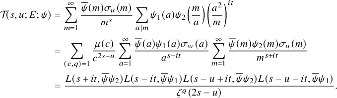 $$ \begin{align*} \mathcal{T}(s, u; E; \psi) & = \sum_{m = 1}^{\infty} \frac{\overline{\psi}(m) \sigma_{u}(m)}{m^{s}} \sum_{a \mid m} \psi_{1}(a) \psi_{2} \left(\frac{m}{a} \right) \left(\frac{a^{2}}{m} \right)^{it}\\ & = \sum_{(c, q) = 1} \frac{\mu(c)}{c^{2s-u}} \sum_{a = 1}^{\infty} \frac{\overline{\psi}(a) \psi_{1}(a) \sigma_{w}(a)}{a^{s-it}} \sum_{m = 1}^{\infty} \frac{\overline{\psi}(m) \psi_{2}(m) \sigma_{u}(m)}{m^{s+it}}\\ & = \frac{L(s+it, \overline{\psi} \psi_{2}) L(s-it, \overline{\psi} \psi_{1}) L(s-u+it, \overline{\psi} \psi_{2}) L(s-u-it, \overline{\psi} \psi_{1})}{\zeta^{q}(2s-u)}. \end{align*} $$
This concludes the proof of Lemma 3.7.
We proceed to compute
by virtue of Lemma 3.7, obtaining
 $$ \begin{align*} \sum_{n = 1}^{\infty} \frac{\overline{\psi}(n) \sigma_{s_{4}-s_{3}}(n) \rho_{f}(\pm n)}{n^{(1-s_{1}+s_{2}-s_{3}+s_{4})/2}} = \epsilon_{f}^{(1 \mp 1)/2} \rho_{f}(1) \frac{L \left(\frac{1-s_{1}+s_{2}+s_{3}-s_{4}}{2}, f \otimes \overline{\psi} \right) L \left(\frac{1-s_{1}+s_{2}-s_{3}+s_{4}}{2}, f \otimes \overline{\psi} \right)}{\zeta^{q}(1-s_{1}+s_{2})}, \end{align*} $$
where $f \in \mathcal {B}_{\kappa }(dq, \psi ^{2})$
. There is beauty in the above quotient since we have
$f \in \mathcal {B}_{\kappa }(dq, \psi ^{2})$
. There is beauty in the above quotient since we have $\zeta ^{q}(1-s_{1}+s_{2})^{-1}$
, which completely cancels out with the term
$\zeta ^{q}(1-s_{1}+s_{2})^{-1}$
, which completely cancels out with the term $\zeta ^{q}(1-s_{1}+s_{2})$
appearing in the expression for
$\zeta ^{q}(1-s_{1}+s_{2})$
appearing in the expression for $\mathcal {J}_{\pm }$
in Proposition 3.3. One can calculate the Dirichlet series for the sum over m in a similar manner, obtaining
$\mathcal {J}_{\pm }$
in Proposition 3.3. One can calculate the Dirichlet series for the sum over m in a similar manner, obtaining
 $$ \begin{align*} \sum_{m = 1}^{\infty} \frac{\psi(m) \overline{\rho_{f}(m)}}{m^{(s_{1}+s_{2}+s_{3}+s_{4}-1)/2}} = \overline{\rho_{f}(1)} L \left(\frac{s_{1}+s_{2}+s_{3}+s_{4}-1}{2}, f \otimes \overline{\psi} \right), \end{align*} $$
where $f \in \mathcal {B}_{\kappa }(dq, \psi ^{2})$
. We obtain the central L-value
$f \in \mathcal {B}_{\kappa }(dq, \psi ^{2})$
. We obtain the central L-value $L(1/2, f \otimes \overline {\psi })^{3}$
if we take the limit
$L(1/2, f \otimes \overline {\psi })^{3}$
if we take the limit $(s_{1}, s_{2}, s_{3}, s_{4}) \mapsto (1/2, 1/2, 1/2, 1/2)$
. A similar procedure can be applied to the Eisenstein contribution to deduce the six Dirichlet L-functions in equation (1.4). The eventual form of the cubic moment side looks like
$(s_{1}, s_{2}, s_{3}, s_{4}) \mapsto (1/2, 1/2, 1/2, 1/2)$
. A similar procedure can be applied to the Eisenstein contribution to deduce the six Dirichlet L-functions in equation (1.4). The eventual form of the cubic moment side looks like
with

Here we set $\mathcal {H}_{\pm }(\chi , \psi ) = \psi (\mp 1) \tau (\psi ) \tau (\overline {\chi \psi }) J(\psi , \psi )$
and used the identity
$\mathcal {H}_{\pm }(\chi , \psi ) = \psi (\mp 1) \tau (\psi ) \tau (\overline {\chi \psi }) J(\psi , \psi )$
and used the identity $\varphi (dq) = d \varphi (q)$
for q prime.
$\varphi (dq) = d \varphi (q)$
for q prime.
3.5.2 Computation of
$\mathcal {E}_{\pm }$

We initially handle
. One can rewrite the direct sum decomposition in equation (2.20) in order to imitate the formulation of Blomer–Milićević [Reference Blomer and Milićeić14], namely
 $$ \begin{align*} \mathcal{B}_{0}(\Gamma_{0}(r^{2})) = \bigsqcup_{r_{1} r_{2} = r^{2}} \bigsqcup_{f \in \mathcal{B}_{0}^{\ast}(\Gamma_{0}(r_{1}))} \bigsqcup_{d \mid r_{2}} \iota_{d} f \cdot \mathbb{C}, \end{align*} $$
where the first two sums are orthogonal, but the last one is not orthogonal and needs to be orthogonalised by Gram–Schmidt. Here we also define
. By [Reference Blomer and Milićeić14, Lemma 9], the set of functions

is an orthonormal basis of the space $\bigsqcup _{d \mid r_{2}} \iota _{d} f \cdot \mathbb {C}$
with
$\bigsqcup _{d \mid r_{2}} \iota _{d} f \cdot \mathbb {C}$
with $f \in \mathcal {B}_{0}^{\ast }(\Gamma _{0}(r_{1}))$
. Then the Fourier coefficients are
$f \in \mathcal {B}_{0}^{\ast }(\Gamma _{0}(r_{1}))$
. Then the Fourier coefficients are
 $$ \begin{align*} \rho_{f^{(g)} \mathfrak{a}}(n) = \sum_{d \mid g} \xi_{g}(d) d^{1/2} \rho_{f \mathfrak{a}} \left(\frac{n}{d} \right) \end{align*} $$
with the convention that $\rho _{f \mathfrak {a}}(x) = 0$
for
$\rho _{f \mathfrak {a}}(x) = 0$
for $x \not \in \mathbb {Z}$
. We calculate the sum over n in equation (3.20) as
$x \not \in \mathbb {Z}$
. We calculate the sum over n in equation (3.20) as
 $$ \begin{align*} \sum_{n = 1}^{\infty} \frac{\psi(n) \sigma_{s_{4}-s_{3}}(n) \rho_{f 0}(\pm n/d)}{n^{(1-s_{1}+s_{2}-s_{3}+s_{4})/2}} = \delta_{d = 1} \epsilon_{f}^{(1 \mp 1)/2} \omega_{f} \rho_{f}(1) \frac{L \left(\!\frac{1-s_{1}+s_{2}+s_{3}-s_{4}}{2}, f \otimes \psi \!\right) L \left(\!\frac{1-s_{1}+s_{2}-s_{3}+s_{4}}{2}, f \otimes \psi \!\right)}{\zeta^{r}(1-s_{1}+s_{2})}, \end{align*} $$
where $\omega _{f}$
stands for the root number for a newform
$\omega _{f}$
stands for the root number for a newform $f \in \mathcal {B}_{0}^{\ast }(\Gamma _{0}(r_{1}))$
. We denote by
$f \in \mathcal {B}_{0}^{\ast }(\Gamma _{0}(r_{1}))$
. We denote by $\psi $
a Dirichlet character modulo r induced by the primitive character
$\psi $
a Dirichlet character modulo r induced by the primitive character $\psi ^{\ast }$
modulo
$\psi ^{\ast }$
modulo $r^{\ast }$
. We regard the character modulo 1 as primitive. Since the central character is trivial and the Hecke eigenvalues are real (Remark 2.10), we use Lemma 2.1 to infer that
$r^{\ast }$
. We regard the character modulo 1 as primitive. Since the central character is trivial and the Hecke eigenvalues are real (Remark 2.10), we use Lemma 2.1 to infer that
 $$ \begin{align*} \sum_{m = 1}^{\infty} \frac{\tau(\psi, m) \overline{\rho_{f}(m/d)}}{m^{(s_{1}+s_{2}+s_{3}+s_{4}-1)/2}} = \frac{\overline{\rho_{f}(1)} \tau(\psi^{\ast}) \psi^{\ast}(d)}{d^{(s_{1}+s_{2}+s_{3}+s_{4}-1)/2}} \Sigma_{r/r^{\ast}}(s_{1}, s_{2}, s_{3}, s_{4}; \psi) L \left(\frac{s_{1}+s_{2}+s_{3}+s_{4}-1}{2}, f \otimes \psi^{\ast} \right), \end{align*} $$
where $\Sigma _{q}(s_{1}, s_{2}, s_{3}, s_{4}; \psi )$
is the multiplicative function
$\Sigma _{q}(s_{1}, s_{2}, s_{3}, s_{4}; \psi )$
is the multiplicative function
 $$ \begin{align*} \sum_{c \mid q} \mu \left(\frac{q}{c} \right) \psi^{\ast} \left(\frac{q}{c} \right) c^{(3-s_{1}-s_{2}-s_{3}-s_{4})/2} \sum_{e \mid c} \mu(e) \psi_{0}(e) \psi^{\ast}(e) e^{(1-s_{1}-s_{2}-s_{3}-s_{4})/2} \lambda_{f} \left(\frac{c}{e} \right) \end{align*} $$
and $\psi _{0}$
is the principal character modulo
$\psi _{0}$
is the principal character modulo $r_{1}$
. On the other hand, we obtain via elementary calculations that
$r_{1}$
. On the other hand, we obtain via elementary calculations that
 $$ \begin{align} \sum_{n \mid r^{\infty}} \frac{\tau(\psi, n) \sigma_{w}(n) \lambda_{f}(n)}{n^{s}} = \tau(\psi^{\ast}) \sum_{c \mid r/r^{\ast}} c \psi^{\ast} \left(\frac{r}{cr^{\ast}} \right) \mu \left(\frac{r}{cr^{\ast}} \right) \sum_{n \mid r^{\infty}} \frac{\psi^{\ast}(n) \sigma_{w}(nc) \lambda_{f}(nc)}{(nc)^{s}}, \end{align} $$
where $s = (1-s_{1}+s_{2}-s_{3}+s_{4})/2$
and
$s = (1-s_{1}+s_{2}-s_{3}+s_{4})/2$
and $w = s_{4}-s_{3}$
. We hence observe that the left-hand side of equation (3.29) equals
$w = s_{4}-s_{3}$
. We hence observe that the left-hand side of equation (3.29) equals $\tau (\psi ^{\ast })$
when
$\tau (\psi ^{\ast })$
when $\psi $
is the quadratic character modulo q or the character modulo
$\psi $
is the quadratic character modulo q or the character modulo $1$
. The problem occurs if
$1$
. The problem occurs if $\psi $
is the principal character modulo a prime q. In this case, a brute force computation gives
$\psi $
is the principal character modulo a prime q. In this case, a brute force computation gives
 $$ \begin{align*} \sum_{c \mid q} c^{1-s} \mu \left(\frac{q}{c} \right) \sum_{n \mid q^{\infty}} \frac{\sigma_{w}(nc) \lambda_{f}(nc)}{n^{s}} = \varphi(q) \left(1-\frac{\lambda_{f}(q)}{q^{s}} \right)^{-1} \left(1-\frac{\lambda_{f}(q)}{q^{s-w}} \right)^{-1}-q. \end{align*} $$
We then conclude that
 $$ \begin{align*} \sum_{n \mid r^{\infty}} \frac{\tau(\psi, n) \sigma_{w}(n) \lambda_{f}(n)}{n^{(1-s_{1}+s_{2}-s_{3}+s_{4})/2}} = \tau(\psi^{\ast}) \Pi_{r/r^{\ast}}(s_{1}, s_{2}, s_{3}, s_{4}; \psi), \end{align*} $$
where $\Pi _{q}(s_{1}, s_{2}, s_{3}, s_{4}; \psi )$
is the multiplicative function
$\Pi _{q}(s_{1}, s_{2}, s_{3}, s_{4}; \psi )$
is the multiplicative function
 $$ \begin{align*} q \sum_{c \mid q} \mu \left(\frac{q}{c} \right) \prod_{p \mid c} \left(1-\frac{\psi^{\ast}(p)}{p} \right) \left(1-\frac{\psi^{\ast}(p) \lambda_{f}(p)}{p^{(1-s_{1}+s_{2}+s_{3}-s_{4})/2}} \right)^{-1} \left(1-\frac{\psi^{\ast}(p) \lambda_{f}(p)}{p^{(1-s_{1}+s_{2}-s_{3}+s_{4})/2}} \right)^{-1}. \end{align*} $$
This reasoning proceeds verbatim for the Eisenstein and holomorphic spectra, giving similar expressions (see [Reference Young70] for an extension of Weisinger’s theory and newform Eisenstein series). Thus we are left with
where

where we define $\mathcal {G}_{\pm }(\chi , \psi ) = \psi (\mp 1) \tau (\psi ) \tau (\psi ^{\ast })^{2} \tau (\overline {\chi } \psi )$
and
$\mathcal {G}_{\pm }(\chi , \psi ) = \psi (\mp 1) \tau (\psi ) \tau (\psi ^{\ast })^{2} \tau (\overline {\chi } \psi )$
and
 $$ \begin{align*} \Omega_{r_{1}, r_{2}}(s_{1}, s_{2}, s_{3}, s_{4}; f; \psi) = \frac{\varphi(r_{1})}{r_{1}^{2}} \sum_{g \mid r_{2}} \xi_{g}(1) &\sum_{d \mid g} \xi_{g}(d) \psi^{\ast}(d) d^{(2-s_{1}-s_{2}-s_{3}-s_{4})/2}\\ &\qquad \times \Sigma_{r/r^{\ast}}(s_{1}, s_{2}, s_{3}, s_{4}; \psi) \Pi_{r/r^{\ast}}(s_{1}, s_{2}, s_{3}, s_{4}; \psi). \end{align*} $$
These terms are complicated, but they are the same size as the main contributions $\mathcal {J}_{\pm }$
in estimations. Thus one can ignore them in the process of using Motohashi’s formula to deduce some moment bounds.
$\mathcal {J}_{\pm }$
in estimations. Thus one can ignore them in the process of using Motohashi’s formula to deduce some moment bounds.
3.6 Endgame: analytic continuation
The aim of this subsection is to show that the spectral decomposition obtained in the preceding subsection can be continued to the whole complex plane $\mathbb {C}^{4}$
and hence to conclude the proof of Theorem 1.1. The main step is identical to that of Motohashi’s monograph [Reference Motohashi55], and we stress the following lemmata:
$\mathbb {C}^{4}$
and hence to conclude the proof of Theorem 1.1. The main step is identical to that of Motohashi’s monograph [Reference Motohashi55], and we stress the following lemmata:
Lemma 3.9 (Motohashi [Reference Motohashi55, Lemma 4.7])
The function $\Xi _{\texttt {s}}(\xi )$
is meromorphic in the domain
$\Xi _{\texttt {s}}(\xi )$
is meromorphic in the domain
 $$ \begin{align*} \mathcal{B}_{4}^{\ast} = \{\xi: \Re(\xi)> -cA \} \times \mathcal{B}_{4} \end{align*} $$
for a fixed small constant $c> 0$
and holomorphic in
$c> 0$
and holomorphic in $\mathcal {B}_{4}^{\ast } \setminus \mathcal {N}$
, where
$\mathcal {B}_{4}^{\ast } \setminus \mathcal {N}$
, where
 $$ \begin{align*} \mathcal{N} = \left\{ (\xi, s_{1}, s_{2}, s_{3}, s_{4})\ : \begin{array}{l} \text{at least one of } \xi+\dfrac{s_{1}+s_{2}+s_{3}+s_{4}-1}{2}, \xi+\dfrac{1-s_{1}+s_{2}+s_{3}-s_{4}}{2}, \\ \ \xi+\dfrac{1-s_{1}+s_{2}-s_{3}+s_{4}}{2} \text{ equals a non-positive integer} \end{array} \right\}. \end{align*} $$
Moreover, if $|\xi |$
tends to infinity in any fixed vertical or horizontal strips while satisfying
$|\xi |$
tends to infinity in any fixed vertical or horizontal strips while satisfying $\Re (\xi )> -cA$
, then we have uniformly in
$\Re (\xi )> -cA$
, then we have uniformly in $\mathcal {B}_{4}$
that
$\mathcal {B}_{4}$
that
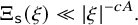 $$ \begin{align} \Xi_{\texttt{s}}(\xi) \ll |\xi|^{-cA}. \end{align} $$
Lemma 3.10 (Motohashi [Reference Motohashi55, Lemma 4.8])
If $(\xi , s_{1}, s_{2}, s_{3}, s_{4})$
is such that the path in equation (3.28) can be drawn in a vertical strip contained in the half plane
$(\xi , s_{1}, s_{2}, s_{3}, s_{4})$
is such that the path in equation (3.28) can be drawn in a vertical strip contained in the half plane $\Re (\tau )> 0$
, then we have that
$\Re (\tau )> 0$
, then we have that
 $$ \begin{align*} \Xi_{\texttt{s}}(\xi) = \frac{\Gamma(\alpha) \Gamma(\beta)}{\Gamma(\gamma)} \int_{0}^{\infty} y^{\xi+(s_{1}+s_{2}+s_{3}+s_{4}-3)/2} G(y, s_{1}) \ {_{2}}F_{1}(\alpha, \beta; \gamma; -y) dy, \end{align*} $$
where $G(y, s)$
is defined in equation (3.4) and
$G(y, s)$
is defined in equation (3.4) and ${_{2}}F_{1}(\alpha , \beta; \gamma; y)$
is the hypergeometric function with
${_{2}}F_{1}(\alpha , \beta; \gamma; y)$
is the hypergeometric function with
 $$ \begin{align*} \alpha = \xi+\frac{1-s_{1}+s_{2}+s_{3}-s_{4}}{2}, \qquad \beta = \xi+\frac{1-s_{1}+s_{2}-s_{3}+s_{4}}{2}, \qquad \gamma = 1+2\xi. \end{align*} $$
We assume that $(s_{1}, s_{2}, s_{3}, s_{4}) \in \mathcal {B}_{4}$
and examine the consequence of Lemma 3.9 for the contribution
$(s_{1}, s_{2}, s_{3}, s_{4}) \in \mathcal {B}_{4}$
and examine the consequence of Lemma 3.9 for the contribution
![]() from Maaß forms. If
from Maaß forms. If $t_{f} \geqslant 3B$
, then
$t_{f} \geqslant 3B$
, then $\Xi _{\texttt {s}}(\pm it_{f})$
is holomorphic and
$\Xi _{\texttt {s}}(\pm it_{f})$
is holomorphic and $\mathrm {O}(t_{f}^{-cA})$
uniformly in
$\mathrm {O}(t_{f}^{-cA})$
uniformly in $\mathcal {B}_{4}$
with an absolute constant c. Hence via Proposition 3.5, the function
$\mathcal {B}_{4}$
with an absolute constant c. Hence via Proposition 3.5, the function $\mathscr {L}^{+} \Psi _{\texttt {s}}^{+}(t_{f})$
is holomorphic and of exponential decay with respect to
$\mathscr {L}^{+} \Psi _{\texttt {s}}^{+}(t_{f})$
is holomorphic and of exponential decay with respect to $t_{f}$
uniformly in
$t_{f}$
uniformly in $\mathcal {B}_{4}$
. This indicates that
$\mathcal {B}_{4}$
. This indicates that
![]() exists as a meromorphic function inside
exists as a meromorphic function inside $\mathcal {B}_{4}$
. The same observation holds for
$\mathcal {B}_{4}$
. The same observation holds for $\mathcal {J}_{+}^{\;\text {hol}}$
. As for the function
$\mathcal {J}_{+}^{\;\text {hol}}$
. As for the function
![]() , we essentially need equation (3.30). From Proposition 3.5, we have
, we essentially need equation (3.30). From Proposition 3.5, we have $\mathscr {L}^{-} \Psi _{\texttt {s}}^{-}(t_{f}) = \mathrm {O}(t_{f}^{-cA})$
uniformly in
$\mathscr {L}^{-} \Psi _{\texttt {s}}^{-}(t_{f}) = \mathrm {O}(t_{f}^{-cA})$
uniformly in $\mathcal {B}_{4}$
provided
$\mathcal {B}_{4}$
provided $t_{f} \geqslant 3B$
. Hence
$t_{f} \geqslant 3B$
. Hence
![]() is meromorphic inside
is meromorphic inside $\mathcal {B}_{4}$
. This discussion works for
$\mathcal {B}_{4}$
. This discussion works for
![]() and
and $\mathcal {E}_{+}^{\;\text {hol}}$
as well.
$\mathcal {E}_{+}^{\;\text {hol}}$
as well.
Thus it remains to contemplate $\mathcal {J}_{\pm }^{\;\text {Eis}}$
and
$\mathcal {J}_{\pm }^{\;\text {Eis}}$
and $\mathcal {E}_{\pm }^{\;\text {Eis}}$
. To this end, we assume first that
$\mathcal {E}_{\pm }^{\;\text {Eis}}$
. To this end, we assume first that $\texttt {s} = (s_{1}, s_{2}, s_{3}, s_{4}) \in \mathcal {E}_{4}$
and set
$\texttt {s} = (s_{1}, s_{2}, s_{3}, s_{4}) \in \mathcal {E}_{4}$
and set
 $$ \begin{align*} \mathcal{J}^{\;\text{Eis}}(\texttt{s}; g; \chi) = \mathcal{J}_{+}^{\;\text{Eis}}(\texttt{s}; g; \chi) + \mathcal{J}_{-}^{\;\text{Eis}}(\texttt{s}; g; \chi). \end{align*} $$
Using Proposition 3.5, one derives
 $$ \begin{align*} \Phi_{\texttt{s}}^{+}(it) &= -\frac{(2\pi)^{s_{1}-s_{2}}}{2i \sinh(\pi t)} \cos \left(\frac{\pi(s_{3}-s_{4})}{2} \right) \Big\{\Xi_{\texttt{s}}(it)-\Xi_{\texttt{s}}(-it) \Big\},\\ \Phi_{\texttt{s}}^{-}(it) &= \frac{(2\pi)^{s_{1}-s_{2}}}{2i \sinh(\pi t)} \left\{\sin \left(\pi \left(\frac{s_{2}-s_{1}}{2}+it \right) \right) \Xi_{\texttt{s}}(it)-\sin \left(\pi \left(\frac{s_{2}-s_{1}}{2}-it \right) \right) \Xi_{\texttt{s}}(-it) \right\}. \end{align*} $$
This yields an expression of $\mathcal {J}^{\;\text {Eis}}(\texttt {s}; g; \chi )$
in terms of
$\mathcal {J}^{\;\text {Eis}}(\texttt {s}; g; \chi )$
in terms of $\Xi _{\texttt {s}}(it)$
. We need to shift the contour in the same way as on pages 170–171 of Motohashi’s monograph [Reference Motohashi55]. This is because
$\Xi _{\texttt {s}}(it)$
. We need to shift the contour in the same way as on pages 170–171 of Motohashi’s monograph [Reference Motohashi55]. This is because $\mathcal {S}_{f}(t; s_{1}, s_{2}, s_{3}, s_{4})$
has poles when
$\mathcal {S}_{f}(t; s_{1}, s_{2}, s_{3}, s_{4})$
has poles when $\psi _{1} = \psi _{2} = \psi $
. The same procedure applies to the term
$\psi _{1} = \psi _{2} = \psi $
. The same procedure applies to the term $\mathcal {E}_{\pm }^{\;\text {Eis}}$
coming from the contribution of the principal character and quadratic character. Gathering these observations, we have proven the following lemma:
$\mathcal {E}_{\pm }^{\;\text {Eis}}$
coming from the contribution of the principal character and quadratic character. Gathering these observations, we have proven the following lemma:
Lemma 3.11. The function $\mathcal {OD}_{4}^{\dagger }$
continues meromorphically to
$\mathcal {OD}_{4}^{\dagger }$
continues meromorphically to $\mathcal {B}_{4}$
, and the decomposition in equation (3.2) holds throughout this domain. In particular, the formula in equation (1.5) is valid for
$\mathcal {B}_{4}$
, and the decomposition in equation (3.2) holds throughout this domain. In particular, the formula in equation (1.5) is valid for $(s_{1}, s_{2}, s_{3}, s_{4}) = (1/2, 1/2, 1/2, 1/2)$
.
$(s_{1}, s_{2}, s_{3}, s_{4}) = (1/2, 1/2, 1/2, 1/2)$
.
This concludes the proof of Theorem 1.1.
4 Implications of Theorem 1.1
In this section, we aim to establish a q-aspect variant of Iwaniec’s short interval fourth moment bound and the twelfth moment bound for Dirichlet L-functions without an average over Dirichlet characters.
4.1 Proofs of Corollaries 1.3 and 1.4
It suffices to specialise the test function in Theorem 1.1 as
 $$ \begin{align} g(t) = \frac{1}{\sqrt{\pi} H} \exp \left(-\left(\frac{t - T}{H} \right)^{2} \right) \end{align} $$
with the parameter H at one’s disposal. We assume that
 $$ \begin{align*} T^{1/2} \leqslant H \leqslant T(\log T)^{-1}. \end{align*} $$
Motohashi [Reference Motohashi55, (5.1.40)–(5.1.42)] evaluated the corresponding integral transform $\Xi $
, and his expression can be used in our context. We then derive an asymptotic formula almost identical to [Reference Motohashi55, Theorem 5.1]. Upon estimating the spectral sum by absolute values, an oscillatory component in the summand evanishes, and we obtain the bound
$\Xi $
, and his expression can be used in our context. We then derive an asymptotic formula almost identical to [Reference Motohashi55, Theorem 5.1]. Upon estimating the spectral sum by absolute values, an oscillatory component in the summand evanishes, and we obtain the bound
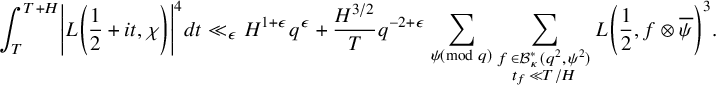 $$ \begin{align} \int_{T}^{T+H} \left|L \left(\frac{1}{2}+it, \chi \right) \right|^{4} dt \ll_{\epsilon} H^{1+\epsilon} q^{\epsilon} + \frac{H^{3/2}}{T} q^{-2+\epsilon} \sum_{\psi\! \pmod q} \sum_{\substack{f \in \mathcal{B}_{\kappa}^{\ast}(q^{2}, \psi^{2}) \\ t_{f} \ll T/H}} L \left(\frac{1}{2}, f \otimes \overline{\psi} \right)^{3}. \end{align} $$
The truncation of the sum is justified since the Taylor expansion of $\exp (-(Ht_{f}/T)^{2}/4)$
in [Reference Motohashi55, (5.1.44)] implies that the rest of the sum is smaller than the main term in equation (4.2). Notice that the central L-values in equation (4.2) are nonnegative, and it thus follows from the work of Petrow–Young [Reference Petrow and Young63, Theorems 1.2 & 1.3] that
$\exp (-(Ht_{f}/T)^{2}/4)$
in [Reference Motohashi55, (5.1.44)] implies that the rest of the sum is smaller than the main term in equation (4.2). Notice that the central L-values in equation (4.2) are nonnegative, and it thus follows from the work of Petrow–Young [Reference Petrow and Young63, Theorems 1.2 & 1.3] that
 $$ \begin{align*} H^{1+\epsilon} q^{\epsilon}+\frac{H^{3/2}}{T} q^{-1+\epsilon} \left(\frac{qT}{H} \right)^{2+\epsilon} \ll H^{1+\epsilon} q^{\epsilon}+\left(\frac{qT}{\sqrt{H}} \right)^{1+\epsilon}. \end{align*} $$
Optimising $H = (qT)^{2/3}$
concludes the proof of Corollaries 1.3 and 1.4.
$H = (qT)^{2/3}$
concludes the proof of Corollaries 1.3 and 1.4.
4.2 Proofs of Corollaries 1.5 and 1.6
This section is devoted to proving the twelfth moment bound. We follow the argument of [Reference Ivić and Motohashi34] verbatim, obtaining the expressionFootnote 6
 $$ \begin{align*} \sum_{r = 1}^{R} \int_{t_{r}}^{t_{r}+T_{0}} \left|L \left(\frac{1}{2}+it, \chi \right) \right|^{4} dt &\ll_{\epsilon} T_{0} q^{-2+\epsilon} \sum_{\psi \pmod{q} } \sum_{\substack{f \in \mathcal{B}_{\kappa}^{\ast}(q^{2}, \psi^{2}) \\ t_{f} \leqslant TT_{0}^{-1} \sqrt{\log T}}} t_{f}^{-1/2} \frac{L(1/2, f \otimes \overline{\psi})^{3}}{L(1, \mathrm{Ad}^{2} f)}\\ & \qquad \times \sum_{r = 1}^{R} t_{r}^{-1/2} \exp \left(-\left(\frac{T_{0} t_{f}}{2t_{r}} \right)^{2} \right) \sin \left(t_{f} \log \frac{t_{f}}{4et_{r}} \right)+RT_{0}(qT)^{\epsilon}. \end{align*} $$
For technical reasons, it is convenient to remove the exponential factor in the last sum over r by partial summation. In doing this, we obtain an error term of $\mathrm {O}_{\epsilon }(RT^{\epsilon } T_{0}^{-1})$
. Then we must majorise
$\mathrm {O}_{\epsilon }(RT^{\epsilon } T_{0}^{-1})$
. Then we must majorise

where

The Cauchy–Schwarz inequality leads one to
 $$ \begin{align*} S_{K} &\leqslant \left(\sum_{\psi \pmod{q} } \sum_{\substack{f \in \mathcal{B}_{\kappa}^{\ast}(q^{2}, \psi^{2}) \\ K \leqslant t_{f} \leqslant 2K}} t_{f}^{-1} \frac{L(1/2, f \otimes \overline{\psi})^{4}}{L(1, \mathrm{Ad}^{2} f)} \right)^{1/2}\\ & \times \left(\sum_{\psi \pmod{q} } \sum_{\substack{f \in \mathcal{B}_{\kappa}^{\ast}(q^{2}, \psi^{2}) \\ K \leqslant t_{f} \leqslant 2K}} \frac{L(1/2, f \otimes \overline{\psi})^{2}}{L(1, \mathrm{Ad}^{2} f)} \left|\sum_{r = 1}^{R} t_{r}^{-1/2-it_{f}} \right|^{2} \right)^{1/2}. \end{align*} $$
Applying the bound of Petrow–Young [Reference Petrow and Young63, Theorem 7.6], the fourth moment is bounded as
 $$ \begin{align*} \sum_{\psi \pmod{q} } \sum_{\substack{f \in \mathcal{B}_{\kappa}^{\ast}(q^{2}, \psi^{2}) \\ K \leqslant t_{f} \leqslant 2K}} t_{f}^{-1} \frac{L(1/2, f \otimes \overline{\psi})^{4}}{L(1, \mathrm{Ad}^{2} f)} \ll_{\epsilon} q^{3+\epsilon} K^{1+\epsilon}. \end{align*} $$
The spectral large sieve in the form involving the square of twisted automorphic L-functions yields
 $$ \begin{align*} \sum_{\psi \pmod{q} } \sum_{\substack{f \in \mathcal{B}_{\kappa}^{\ast}(q^{2}, \psi^{2}) \\ K \leqslant t_{f} \leqslant 2K}} \frac{L(1/2, f \otimes \overline{\psi})^{2}}{L(1, \mathrm{Ad}^{2} f)} \left|\sum_{r = 1}^{R} t_{r}^{-1/2-it_{f}} \right|^{2} \ll_{\epsilon} q^{3+\epsilon} RKT^{\epsilon} T_{0}^{-1}, \end{align*} $$
since $K \ll TT_{0}^{-1} \sqrt {\log T}$
. It follows that
$K \ll TT_{0}^{-1} \sqrt {\log T}$
. It follows that
 $$ \begin{align*} S_{K} \ll_{\epsilon} q^{3+\epsilon} R^{1/2} K^{1+\epsilon} T^{\epsilon} T_{0}^{-1/2} \end{align*} $$
and the summation over K eventually gives
 $$ \begin{align*} \sum_{r = 1}^{R} \int_{t_{r}}^{t_{r}+T_{0}} \left|L \left(\frac{1}{2}+it, \chi \right) \right|^{4} dt \ll_{\epsilon} \left(RT_{0}+qT \sqrt{\frac{R}{T_{0}}} \right)(qT)^{\epsilon}. \end{align*} $$
This establishes Corollary 1.5. Corollary 1.6 follows from Jutila’s trick described in [Reference Jutila42, §6].
A Twists of Maaß newforms
We evaluate the size of the conductor of $f \otimes \overline {\psi }$
via automorphic representation theory.
$f \otimes \overline {\psi }$
via automorphic representation theory.
Theorem A.1. Let $\psi $
be a primitive character modulo an odd squarefree q and
$\psi $
be a primitive character modulo an odd squarefree q and $d \mid q$
. Let
$d \mid q$
. Let $f \in \mathcal {B}_{\kappa }^{\ast }(dq, \psi ^{2})$
be a Hecke–Maaß newform. Then the twist
$f \in \mathcal {B}_{\kappa }^{\ast }(dq, \psi ^{2})$
be a Hecke–Maaß newform. Then the twist $f \otimes \overline {\psi }$
has conductor
$f \otimes \overline {\psi }$
has conductor $q^{2}$
if
$q^{2}$
if $\psi $
is nonquadratic. If
$\psi $
is nonquadratic. If $\psi $
is quadratic, then
$\psi $
is quadratic, then $f \otimes \overline {\psi }$
has conductor dividing
$f \otimes \overline {\psi }$
has conductor dividing $q^{2}$
, and all three possibilities occur: if
$q^{2}$
, and all three possibilities occur: if $d = 1$
, then the conductor is
$d = 1$
, then the conductor is $q^{2}$
; and if
$q^{2}$
; and if $d = q$
, then
$d = q$
, then
 $$ \begin{align*} \mathrm{cond}(f \otimes \overline{\psi}) = \begin{cases} 1 & \text{if } f \text{ corresponds to a principal series representation},\\ q & \text{if } f \text{ corresponds to a special representation},\\ q^{2} & \text{if } f \text{ corresponds to a twist-minimal representation}. \end{cases} \end{align*} $$
An automorphic representation f is named twist-minimal if it has minimal conductor among all their twists $f \otimes \psi $
by Dirichlet characters, namely
$f \otimes \psi $
by Dirichlet characters, namely $\mathrm {cond}(f) \leqslant \mathrm {cond}(f \otimes \psi )$
. Theorem A.1 asserts in particular that
$\mathrm {cond}(f) \leqslant \mathrm {cond}(f \otimes \psi )$
. Theorem A.1 asserts in particular that $f \otimes \overline {\psi }$
has conductor
$f \otimes \overline {\psi }$
has conductor $q^{2}$
when f corresponds to a twist-minimal representation at the primes dividing q. This matches work of Booker–Lee–Strömbersson [Reference Booker, Lee and Strömbergsson16, Lemma 1.4]. The method to show Theorem A.1 features the use of automorphic representation theory. Nonetheless, one can also use the local Langlands correspondence and tend toward the Galois side. The only way the conductor of the tensor product could be smaller than
$q^{2}$
when f corresponds to a twist-minimal representation at the primes dividing q. This matches work of Booker–Lee–Strömbersson [Reference Booker, Lee and Strömbergsson16, Lemma 1.4]. The method to show Theorem A.1 features the use of automorphic representation theory. Nonetheless, one can also use the local Langlands correspondence and tend toward the Galois side. The only way the conductor of the tensor product could be smaller than $q^{2}$
is if the associated representation has a subrepresentation as an inertia representation isomorphic to
$q^{2}$
is if the associated representation has a subrepresentation as an inertia representation isomorphic to $\psi $
, in which case it has a quotient representation also isomorphic to
$\psi $
, in which case it has a quotient representation also isomorphic to $\psi $
since its determinant is
$\psi $
since its determinant is $\psi ^2$
. Consequently, f is not twist-minimal if the conductor
$\psi ^2$
. Consequently, f is not twist-minimal if the conductor $\mathrm {cond}(f \otimes \overline {\psi })$
does not equal
$\mathrm {cond}(f \otimes \overline {\psi })$
does not equal $q^{2}$
, and there are no twist-minimal principal series representations in our context.
$q^{2}$
, and there are no twist-minimal principal series representations in our context.
A.1 Classification of representations
Let $\pi _{v}$
be a generic irreducible admissible representation of
$\pi _{v}$
be a generic irreducible admissible representation of $\operatorname {\mathrm {GL}}_{2}(\mathbb {Q}_{v})$
with central character
$\operatorname {\mathrm {GL}}_{2}(\mathbb {Q}_{v})$
with central character $\omega _{v}$
. We recall that such representations can be classified into principal series representations, special representations or supercuspidal representations. Standard references for the properties of these representations are [Reference Bump20, Reference Goldfeld and Hundley25], and the articles [Reference Humphries32, Reference Schmidt66] discuss the conductor exponents of these representations.
$\omega _{v}$
. We recall that such representations can be classified into principal series representations, special representations or supercuspidal representations. Standard references for the properties of these representations are [Reference Bump20, Reference Goldfeld and Hundley25], and the articles [Reference Humphries32, Reference Schmidt66] discuss the conductor exponents of these representations.
A.1.1 Principal series representations of
$\operatorname {\mathrm {GL}}_{2}(\mathbb {Q}_{v})$

A principal series representation $\pi _{v}$
is unitarily induced from a representation of the Borel subgroup of
$\pi _{v}$
is unitarily induced from a representation of the Borel subgroup of $\operatorname {\mathrm {GL}}_{2}(\mathbb {Q}_{v})$
, and these representations are indexed by two characters
$\operatorname {\mathrm {GL}}_{2}(\mathbb {Q}_{v})$
, and these representations are indexed by two characters
 $$ \begin{align*} \omega_{p, 1} = \beta_{p, 1} |\cdot|_{v}^{s_{1}}, \qquad \omega_{p, 2} = \beta_{p, 2} |\cdot|_{v}^{s_{2}} \end{align*} $$
of $\mathbb {Q}_{v}^{\times }$
, where
$\mathbb {Q}_{v}^{\times }$
, where $\beta _{p, 1}$
and
$\beta _{p, 1}$
and $\beta _{p, 2}$
are characters of
$\beta _{p, 2}$
are characters of $\mathcal {O}_{v}^{\times }$
and
$\mathcal {O}_{v}^{\times }$
and $s_{1}, s_{2} \in \mathbb {C}$
. We write
$s_{1}, s_{2} \in \mathbb {C}$
. We write
 $$ \begin{align*} \pi_{v} \cong \omega_{p, 1} \boxplus \omega_{p, 2}. \end{align*} $$
This representation is irreducible and unitarisable if and only if either $s_{1}, s_{2} \in i\mathbb {R}$
or
$s_{1}, s_{2} \in i\mathbb {R}$
or $s_{1}+s_{2} \in i\mathbb {R}$
with
$s_{1}+s_{2} \in i\mathbb {R}$
with $s_{1}-s_{2} \in (-1, 1)$
and
$s_{1}-s_{2} \in (-1, 1)$
and $\beta _{p, 1} = \beta _{p, 2}$
. The central character of
$\beta _{p, 1} = \beta _{p, 2}$
. The central character of $\pi _{v}$
is
$\pi _{v}$
is
 $$ \begin{align*} \omega_{\pi_{v}} = \omega_{p, 1} \omega_{p, 2} = \beta_{p, 1} \beta_{p, 2} |\cdot|_{v}^{s_{1}+s_{2}}. \end{align*} $$
The conductor exponent $c(\pi _{v})$
equals
$c(\pi _{v})$
equals $c(\omega _{p, 1})+c(\omega _{p, 2})$
. If
$c(\omega _{p, 1})+c(\omega _{p, 2})$
. If $\omega _{v}^{\prime }$
is a character of
$\omega _{v}^{\prime }$
is a character of $\mathbb {Q}_{v}^{\times }$
, the twist of
$\mathbb {Q}_{v}^{\times }$
, the twist of $\pi _{v}$
by
$\pi _{v}$
by $\omega _{v}^{\prime }$
is the principal series representation
$\omega _{v}^{\prime }$
is the principal series representation
 $$ \begin{align*} \pi_{v} \otimes \omega_{v}^{\prime} \cong \omega_{p, 1} \omega_{v}^{\prime} \boxplus \omega_{p, 2} \omega_{v}^{\prime}. \end{align*} $$
If $\pi _{v}$
has trivial central character, then
$\pi _{v}$
has trivial central character, then $\omega _{p, 2} = \omega _{p, 1}^{-1}$
so that
$\omega _{p, 2} = \omega _{p, 1}^{-1}$
so that $\beta _{p, 2} = \beta _{p, 1}^{-1}$
,
$\beta _{p, 2} = \beta _{p, 1}^{-1}$
, $s_{2} = -s_{1}$
and
$s_{2} = -s_{1}$
and $c(\pi _{v}) = 2c(\omega _{p, 1})$
.
$c(\pi _{v}) = 2c(\omega _{p, 1})$
.
A.1.2 Special representations of
$\operatorname {\mathrm {GL}}_{2}(\mathbb {Q}_{v})$

A special representation is a twist of the Steinberg representation: it is the irreducible subrepresentation
 $$ \begin{align*} \pi_{v} \cong \omega_{v} \mathrm{St}_{v} \end{align*} $$
of codimension one of the reducible principal series representation $\omega _{v} |\cdot |_{v}^{1/2} \boxplus \omega _{v} |\cdot |_{v}^{-1/2}$
, where
$\omega _{v} |\cdot |_{v}^{1/2} \boxplus \omega _{v} |\cdot |_{v}^{-1/2}$
, where $\omega _{v} = \beta _{v} |\cdot |_{v}^{s}$
is a central character of
$\omega _{v} = \beta _{v} |\cdot |_{v}^{s}$
is a central character of $\mathbb {Q}_{v}^{\times }$
with
$\mathbb {Q}_{v}^{\times }$
with $\beta _{v}$
a character of
$\beta _{v}$
a character of $\mathcal {O}_{v}^{\times }$
and
$\mathcal {O}_{v}^{\times }$
and $s \in \mathbb {C}$
. The central character of
$s \in \mathbb {C}$
. The central character of $\pi _{v}$
is
$\pi _{v}$
is
 $$ \begin{align*} \omega_{\pi_{v}} = \omega_{v}^{2} = \beta_{v}^{2} |\cdot|_{v}^{2s}. \end{align*} $$
The conductor exponent is
 $$ \begin{align*} c(\pi_{v}) = \begin{cases} 1 & \text{if } c(\omega_{v}) = 0,\\ 2c(\omega_{v}) & \text{otherwise}. \end{cases} \end{align*} $$
If $\omega _{v}^{\prime }$
is a character of
$\omega _{v}^{\prime }$
is a character of $\mathbb {Q}_{v}^{\times }$
, the twist of
$\mathbb {Q}_{v}^{\times }$
, the twist of $\pi _{v}$
by
$\pi _{v}$
by $\omega _{v}^{\prime }$
is the special representation
$\omega _{v}^{\prime }$
is the special representation
 $$ \begin{align*} \pi_{v} \otimes \omega_{v}^{\prime} = \omega_{v} \omega_{v}^{\prime} \mathrm{St}_{v}. \end{align*} $$
A.1.3 Supercuspidal representations of
$\operatorname {\mathrm {GL}}_{2}(\mathbb {Q}_{v})$

A supercuspidal representation is the compact induction of a finite-dimensional representation $\rho _{\pi _{v}}$
of a maximal open subgroup H of
$\rho _{\pi _{v}}$
of a maximal open subgroup H of $\operatorname {\mathrm {GL}}_{2}(\mathbb {Q}_{v})$
such that H is compact modulo the centre
$\operatorname {\mathrm {GL}}_{2}(\mathbb {Q}_{v})$
such that H is compact modulo the centre $Z(\mathbb {Q}_{v})$
. Every maximal open subgroup of
$Z(\mathbb {Q}_{v})$
. Every maximal open subgroup of $\operatorname {\mathrm {GL}}_{2}(\mathbb {Q}_{v})$
that is compact modulo the centre is conjugate to either
$\operatorname {\mathrm {GL}}_{2}(\mathbb {Q}_{v})$
that is compact modulo the centre is conjugate to either $Z(\mathbb {Q}_{v}) \operatorname {\mathrm {GL}}_{2}(\mathcal {O}_{v})$
or
$Z(\mathbb {Q}_{v}) \operatorname {\mathrm {GL}}_{2}(\mathcal {O}_{v})$
or $NK_{0}(\mathfrak {p}_{v})$
, the normaliser of
$NK_{0}(\mathfrak {p}_{v})$
, the normaliser of $K_{0}(\mathfrak {p}_{v})$
in
$K_{0}(\mathfrak {p}_{v})$
in $\operatorname {\mathrm {GL}}_{2}(\mathbb {Q}_{v})$
, where
$\operatorname {\mathrm {GL}}_{2}(\mathbb {Q}_{v})$
, where $\mathfrak {p}_{v}$
is the maximal ideal of the ring of integers
$\mathfrak {p}_{v}$
is the maximal ideal of the ring of integers $\mathcal {O}_{v}$
of
$\mathcal {O}_{v}$
of $\mathbb {Q}_{v}$
. A supercuspidal representation
$\mathbb {Q}_{v}$
. A supercuspidal representation $\pi _{v}$
is said to be of type I if H is conjugate to
$\pi _{v}$
is said to be of type I if H is conjugate to $Z(\mathbb {Q}_{v}) \operatorname {\mathrm {GL}}_{2}(\mathcal {O}_{v})$
and of type II if H is conjugate to
$Z(\mathbb {Q}_{v}) \operatorname {\mathrm {GL}}_{2}(\mathcal {O}_{v})$
and of type II if H is conjugate to $NK_{0}(\mathfrak {p}_{v})$
. Supercuspidal representations always have conductor exponent
$NK_{0}(\mathfrak {p}_{v})$
. Supercuspidal representations always have conductor exponent $c(\pi _{v}$
) at least 2. The twist
$c(\pi _{v}$
) at least 2. The twist $\pi _{v} \otimes \omega _{v}^{\prime }$
of
$\pi _{v} \otimes \omega _{v}^{\prime }$
of $\pi _{v}$
by a character
$\pi _{v}$
by a character $\omega _{v}^{\prime }$
of
$\omega _{v}^{\prime }$
of $\mathbb {Q}_{v}^{\times }$
is also a supercuspidal representation.
$\mathbb {Q}_{v}^{\times }$
is also a supercuspidal representation.
A.2 Proof of Theorem A.1
A representation $\pi $
of
$\pi $
of $\mathrm {GL}_{2}(F)$
(where F is a nonarchimedean local field) of conductor
$\mathrm {GL}_{2}(F)$
(where F is a nonarchimedean local field) of conductor $1$
, or equivalently of conductor exponent
$1$
, or equivalently of conductor exponent $c(\pi ) = 0$
, must be a spherical principal series representation
$c(\pi ) = 0$
, must be a spherical principal series representation $\pi = \omega _{1} \boxplus \omega _{2}$
with both characters
$\pi = \omega _{1} \boxplus \omega _{2}$
with both characters $\omega _{1}, \omega _{2}$
of
$\omega _{1}, \omega _{2}$
of $F^{\times }$
unramified, or equivalently of conductor exponent
$F^{\times }$
unramified, or equivalently of conductor exponent $c(\omega _{1}) = c(\omega _{2}) = 0$
. The central character is
$c(\omega _{1}) = c(\omega _{2}) = 0$
. The central character is $\omega _{\pi } = \omega _{1} \omega _{2}$
, which has conductor exponent
$\omega _{\pi } = \omega _{1} \omega _{2}$
, which has conductor exponent $c(\omega _{1} \omega _{2}) = 0$
; if this central character is trivial, then
$c(\omega _{1} \omega _{2}) = 0$
; if this central character is trivial, then $\omega _{2} = \omega _{1}^{-1}$
. It holds that
$\omega _{2} = \omega _{1}^{-1}$
. It holds that $\omega _{1}(x) = |x|_{v}^{it_{v}}$
and
$\omega _{1}(x) = |x|_{v}^{it_{v}}$
and $\omega _{2}(x) = |x|_{v}^{-it_{v}}$
, where
$\omega _{2}(x) = |x|_{v}^{-it_{v}}$
, where $t_{v}$
is such that the Hecke eigenvalue is
$t_{v}$
is such that the Hecke eigenvalue is $\lambda _{\pi }(p) = p^{it_{v}}+p^{-it_{v}}$
. We must think of this as being the local component of f at a prime not dividing the level.
$\lambda _{\pi }(p) = p^{it_{v}}+p^{-it_{v}}$
. We must think of this as being the local component of f at a prime not dividing the level.
For conductor p, or equivalently conductor exponent $c(\pi ) = 1$
, there are two possibilities. The first is that
$c(\pi ) = 1$
, there are two possibilities. The first is that $\pi $
is a special representation
$\pi $
is a special representation $\omega \mathrm {St}$
, where
$\omega \mathrm {St}$
, where $\omega $
is an unramified character (so that
$\omega $
is an unramified character (so that $c(\omega ) = 0$
). The central character is
$c(\omega ) = 0$
). The central character is $\omega _{\pi } = \omega ^{2}$
that has conductor exponent
$\omega _{\pi } = \omega ^{2}$
that has conductor exponent $c(\omega ^{2}) = 0$
. We must think of this as the local component of f at a prime that exactly divides the level and such that the prime does not divide the conductor of the central character of f. The other possibility is that
$c(\omega ^{2}) = 0$
. We must think of this as the local component of f at a prime that exactly divides the level and such that the prime does not divide the conductor of the central character of f. The other possibility is that $\pi = \omega _{1} \boxplus \omega _{2}$
is a nonspherical principal series representations, where either
$\pi = \omega _{1} \boxplus \omega _{2}$
is a nonspherical principal series representations, where either $c(\omega _{1}) = 1$
and
$c(\omega _{1}) = 1$
and $c(\omega _{2}) = 0$
or vice versa. The central character is
$c(\omega _{2}) = 0$
or vice versa. The central character is $\omega _{\pi } = \omega _{1} \omega _{2}$
that has conductor exponent
$\omega _{\pi } = \omega _{1} \omega _{2}$
that has conductor exponent $c(\omega _{1} \omega _{2}) = 1$
. We must think of this as the local component of f at a prime that exactly divides the level and such that the prime also divides the conductor of the central character.
$c(\omega _{1} \omega _{2}) = 1$
. We must think of this as the local component of f at a prime that exactly divides the level and such that the prime also divides the conductor of the central character.
For conductor $p^{r}$
with
$p^{r}$
with $r \geqslant 2$
, or equivalently conductor exponent
$r \geqslant 2$
, or equivalently conductor exponent $c(\pi ) = r$
, there are three possibilities. The first possibility is that
$c(\pi ) = r$
, there are three possibilities. The first possibility is that $\pi = \omega _{1} \boxplus \omega _{2}$
is a nonspherical principal series representation for which
$\pi = \omega _{1} \boxplus \omega _{2}$
is a nonspherical principal series representation for which $r = c(\pi ) = c(\omega _{1})+c(\omega _{2}) = r$
. The central character is
$r = c(\pi ) = c(\omega _{1})+c(\omega _{2}) = r$
. The central character is $\omega _{\pi } = \omega _{1} \omega _{2}$
that has conductor exponent at most r. The second possibility is that
$\omega _{\pi } = \omega _{1} \omega _{2}$
that has conductor exponent at most r. The second possibility is that $\pi = \omega \mathrm {St}$
is a special representation, where
$\pi = \omega \mathrm {St}$
is a special representation, where $\omega $
is a ramified character, so that
$\omega $
is a ramified character, so that $c(\omega ) \geqslant 1$
and
$c(\omega ) \geqslant 1$
and $r = c(\pi ) = 2c(\omega )$
(so that r is necessarily even). The central character is
$r = c(\pi ) = 2c(\omega )$
(so that r is necessarily even). The central character is $\omega _{\pi } = \omega ^{2}$
that has conductor exponent at most r. The third possibility is that
$\omega _{\pi } = \omega ^{2}$
that has conductor exponent at most r. The third possibility is that $\pi $
is supercuspidal.
$\pi $
is supercuspidal.
The twist by $\chi $
of a principal series representation
$\chi $
of a principal series representation $\pi = \omega _{1} \boxplus \omega _{2}$
with central character
$\pi = \omega _{1} \boxplus \omega _{2}$
with central character $\omega _{\pi } = \omega _{1} \omega _{2}$
is
$\omega _{\pi } = \omega _{1} \omega _{2}$
is $\pi \otimes \chi = \omega _{1} \chi \boxplus \omega _{2} \chi $
with central character
$\pi \otimes \chi = \omega _{1} \chi \boxplus \omega _{2} \chi $
with central character $\omega _{\pi \otimes \chi } = \omega _{1} \omega _{2} \chi ^{2}$
. The conductor exponent of
$\omega _{\pi \otimes \chi } = \omega _{1} \omega _{2} \chi ^{2}$
. The conductor exponent of $\pi \otimes \chi $
becomes
$\pi \otimes \chi $
becomes $c(\pi \otimes \chi ) = c(\omega _{1} \chi ) + c(\omega _{2} \chi )$
, and the conductor exponent of
$c(\pi \otimes \chi ) = c(\omega _{1} \chi ) + c(\omega _{2} \chi )$
, and the conductor exponent of $\omega _{\pi \otimes \chi }$
becomes
$\omega _{\pi \otimes \chi }$
becomes $c(\omega _{1} \omega _{2} \chi ^{2})$
. The twist of a special representation
$c(\omega _{1} \omega _{2} \chi ^{2})$
. The twist of a special representation $\pi = \omega \mathrm {St}$
with central character
$\pi = \omega \mathrm {St}$
with central character $\omega _{\pi } = \omega ^{2}$
is
$\omega _{\pi } = \omega ^{2}$
is $\pi \otimes \chi = \omega \chi \mathrm {St}$
with central character
$\pi \otimes \chi = \omega \chi \mathrm {St}$
with central character $\omega _{\pi \otimes \chi } = \omega ^{2} \chi ^{2}$
. The conductor exponent of
$\omega _{\pi \otimes \chi } = \omega ^{2} \chi ^{2}$
. The conductor exponent of $\pi \otimes \chi $
becomes
$\pi \otimes \chi $
becomes $c(\pi \otimes \chi ) = \max \{1, 2c(\omega \chi ) \}$
, and the conductor exponent of
$c(\pi \otimes \chi ) = \max \{1, 2c(\omega \chi ) \}$
, and the conductor exponent of $\omega _{\pi \otimes \chi }$
becomes
$\omega _{\pi \otimes \chi }$
becomes $c(\omega ^2 \chi ^2)$
.
$c(\omega ^2 \chi ^2)$
.
Proof of Theorem A.1
The proof uses representation theory, and it suffices to prove Theorem A.1 when $q = p$
is prime. Given a newform f of level
$q = p$
is prime. Given a newform f of level $dq$
and central character
$dq$
and central character $\psi ^{2}$
, there is a cuspidal automorphic representation
$\psi ^{2}$
, there is a cuspidal automorphic representation $\pi = \pi _{\infty } \otimes \bigotimes _{v} \pi _{v}$
of
$\pi = \pi _{\infty } \otimes \bigotimes _{v} \pi _{v}$
of $\operatorname {\mathrm {GL}}_{2}(\mathbb {A}_{\mathbb {Q}})$
, unique up to isomorphism, with conductor exponent
$\operatorname {\mathrm {GL}}_{2}(\mathbb {A}_{\mathbb {Q}})$
, unique up to isomorphism, with conductor exponent $c(\pi _{v})$
at each prime p satisfying
$c(\pi _{v})$
at each prime p satisfying $p^{c(\pi _{v})} \parallel dq$
, whose central character
$p^{c(\pi _{v})} \parallel dq$
, whose central character $\omega _{\pi }$
is the idèlic lift of the primitive character
$\omega _{\pi }$
is the idèlic lift of the primitive character $\chi $
that induces
$\chi $
that induces $\psi ^{2}$
and whose global newvector
$\psi ^{2}$
and whose global newvector $\xi ^{\circ }$
is the adèlic lift of f. If
$\xi ^{\circ }$
is the adèlic lift of f. If $p \nmid dq$
, then
$p \nmid dq$
, then $\pi _{v}$
is spherical and the local conductor exponents ought to satisfy
$\pi _{v}$
is spherical and the local conductor exponents ought to satisfy $c(\pi _{v}) = 0$
. All the action happens when
$c(\pi _{v}) = 0$
. All the action happens when $p \mid dq$
for which
$p \mid dq$
for which $\pi _{v}$
is ramified. The central character
$\pi _{v}$
is ramified. The central character $\omega _{\pi _{v}}$
is the local component
$\omega _{\pi _{v}}$
is the local component $\omega _{v}^{2}$
of the idèlic lift of
$\omega _{v}^{2}$
of the idèlic lift of $\chi $
, and the local conductor exponent
$\chi $
, and the local conductor exponent $c(\omega _{v})$
is such that
$c(\omega _{v})$
is such that $p^{c(\omega _{v})} \parallel q$
. If
$p^{c(\omega _{v})} \parallel q$
. If $\omega _{v}$
is nonquadratic, then
$\omega _{v}$
is nonquadratic, then $c(\omega _{\pi _{v}}) = c(\omega _{v}^2) = c(\omega _{v})$
; however, if
$c(\omega _{\pi _{v}}) = c(\omega _{v}^2) = c(\omega _{v})$
; however, if $\omega _{v}$
is quadratic, then
$\omega _{v}$
is quadratic, then $c(\omega _{\pi _{v}}) = 0$
, where
$c(\omega _{\pi _{v}}) = 0$
, where $c(\omega _{v}) = 1$
. The accurate quantity of the conductor exponent
$c(\omega _{v}) = 1$
. The accurate quantity of the conductor exponent $c(\pi _{v} \otimes \chi _{v})$
is calculable for given
$c(\pi _{v} \otimes \chi _{v})$
is calculable for given $\pi _{v}$
, where
$\pi _{v}$
, where $\chi _{v}$
is the character corresponding to
$\chi _{v}$
is the character corresponding to $\overline {\psi }$
. It follows that
$\overline {\psi }$
. It follows that $\mathrm {cond}(f \otimes \overline {\psi }) \mid q^{2}$
with equality if f is twist-minimal or
$\mathrm {cond}(f \otimes \overline {\psi }) \mid q^{2}$
with equality if f is twist-minimal or $d = 1$
via Lemma 1.4 of [Reference Booker, Lee and Strömbergsson16]. Since
$d = 1$
via Lemma 1.4 of [Reference Booker, Lee and Strömbergsson16]. Since $\pi _{v}$
is a generic irreducible admissible representation of
$\pi _{v}$
is a generic irreducible admissible representation of $\operatorname {\mathrm {GL}}_{2}(\mathbb {Q}_{v})$
, one must go through a case-by-case analysis. Using the above classification, the local conductor exponents can be calculated, although one cannot deal with all the cases in one fell swoop.
$\operatorname {\mathrm {GL}}_{2}(\mathbb {Q}_{v})$
, one must go through a case-by-case analysis. Using the above classification, the local conductor exponents can be calculated, although one cannot deal with all the cases in one fell swoop.
-
1. The case where
$\psi $
is quadratic:-
(a) If
$d = 1$
, then
$\pi _{v} \cong \omega _{v} \mathrm {St}_{v}$
for some unramified character
$\omega _{v}$
of
$\mathbb {Q}_{v}^{\times }$
by the above classification. The local component of the twist
$f \otimes \overline {\psi }$
is
$\pi _{v} \otimes \chi _{v} \cong \omega _{v} \chi _{v} \mathrm {St}_{v}$
. The conductor exponent of
$\pi _{v} \otimes \chi _{v}$
thus equals
$2$
, which means that
$f \otimes \overline {\psi }$
has conductor
$p^{2}$
. -
(b) If
$d = q$
is a prime p, then
$\pi _{v}$
has conductor exponent
$c(\pi _{v}) = 2$
. Since
$\omega _{\pi _{v}}$
is trivial,
$\pi _{v}$
can either be principal series, special or supercuspidal. Humphries [Reference Humphries32] discusses this problem in detail and classifies everything in a comprehensive manner. The crucial point is that if
$\pi _{v} = \omega _{p, \mathrm {quad}} \boxplus \omega _{p, \mathrm {quad}}$
, where
$\omega _{p, \mathrm {quad}}$
denotes the quadratic character of conductor exponent
$1$
, then
$\pi _{v} \otimes \chi _{v}$
is a spherical principal series representation of conductor exponent
$0$
, so that
$f \otimes \overline {\psi }$
has conductor
$1$
. If
$\pi _{v} = \omega _{v} \mathrm {St}_{v}$
is special, its twist is a special representation of conductor exponent
$1$
, so that
$f \otimes \overline {\psi }$
has conductor p. In all other cases,
$\pi _{v}$
is twist-minimal and
$\pi _{v} \otimes \chi _{v}$
has conductor exponent
$2$
, so that
$f \otimes \overline {\psi }$
has conductor
$p^{2}$
.
-
-
2. The case where
$\psi $
is nonquadratic:-
(a) We first handle the case
$d = 1$
. Since
$\psi ^{2}$
is primitive modulo p, the corresponding character
$\omega _{\pi _{v}}$
has conductor exponent
$c(\omega _{\pi _{v}}) = 1$
. By the above classification,
$\pi _{v} = \omega _{p, 1} \boxplus \omega _{p, 2}$
, where
$c(\omega _{p, 1}) = 1$
,
$c(\omega _{p, 2}) = 0$
and
$\omega _{\pi _{v}} = \omega _{p, 1} \omega _{p, 2}$
. The twist is
$\pi _{v} \otimes \chi _{v} = \omega _{p, 1} \chi _{v} \boxplus \omega _{p, 2} \chi _{v}$
. Since
$\omega _{p, 1} \omega _{p, 2} = \chi _{v}^{-2}$
(recall f has central character
$\psi ^{2}$
), we must have
$\omega _{p, 1} \chi _{v} = \omega _{p, 2}^{-1} \chi _{v}^{-1}$
, which has conductor exponent
$1$
, as does
$\omega _{p, 2} \chi _{v}$
. Hence the conductor exponent of
$\pi _{v} \otimes \chi _{v}$
is
$c(\omega _{p, 1} \chi _{v})+c(\omega _{p, 2} \chi _{v}) = 2$
, which means that
$f \otimes \overline {\psi }$
has conductor
$p^{2}$
. -
(b) If
$d = p$
, then
$\pi _{v}$
has conductor exponent
$c(\pi _{v}) = 2$
. All three possibilities for
$\pi _{v}$
are open, and one can check in each case that twisting leaves its conductor exponent unchanged.
-


This concludes the proof of Theorem A.1.
Acknowledgments
The author expresses his gratitude to Eren Mehmet Kıral for supervising this work. He also thanks Valentin Blomer, Jack Buttcane, Paul Nelson and Peter Sarnak for having an interest in earlier versions of this article. Appendix A is attributed to Peter Humphries, and the author acknowledges his diversified comments that improved the readability of this article. Special thanks are owed to Alexandre Perozim de Faveri, Yoichi Motohashi, Maksym Radziwiłł and Will Sawin for their assistance.
Conflicts of Interest
None.
Financial Support
The author acknowledges the support of the Masason Foundation and the Spirit of Ramanujan STEM Talent Initiative.


 Open access