Introduction

In order to predict avalanche run-out distances, models of avalanche dynamics have utilized linear and non-linear fluid constitutive representations (Reference SalmSalm, 1966; Reference Perla, Cheng and McClungPerla and others, 1980; Reference Dent and LangDent and Lang, 1983). Unfortunately, many of these constitutive models have not worked well because they contain parameters that are not easily measured. To use the models, they must first be “calibrated” by modeling known avalanches. Model parameters are back-calculated by matching speeds and final run-out positions. These model parameters must then be correlated with avalanche type, size and terrain until enough experience is gained to allow the parameters to be estimated for different kinds of avalanches. This procedure permits virtually any model to be “calibrated”. It also presents difficulties in new or unique situations. Lately, other less empirical models of avalanche motion have been proposed. These models are based upon mechanical properties of snow that can be measured. Most notable are the granular-flow models, which treat an avalanche as a collection of individual snow grains (Reference DentDent, 1986, Reference Dent1993; Reference Savage and HutterSavage and Hutter, 1991). However, due to a lack of detailed flow information, evaluation of these models is also difficult. In order to build better models of snow-avalanche motion, more information about that motion needs to be gathered.

Revolving Door Avalanche Path

An avalanche-experiment facility has been constructed on the Revolving Door avalanche path (Fig. 1) near the Bridger Bowl ski area in southwestern Montana. The path is about 100 m long on a nearly uniform 35° east-facing slope. A bowl-shaped starting zone provides snow for avalanches of up to 1.5 m deep and 1000 m³ in volume. Near the middle and slightly off to one side of this avalanche path, an instrument shed has been constructed behind the protection of a large automobile-sized rock. The shed is about 2.5 m square and 2 m high. Both the rock and the shed become mostly buried by the mid-winter snowpack. By removing snow from the track beside the rock and wall of the instrument shed, the top 60 cm of one wall of the shed parallel to the avalanche-flow direction can be exposed to avalanches as they descend the Revolving Door path. An explosive charge in the avalanche-starting zone is used to trigger avalanches which flow down the path, over the buried rock, and along the exposed wall of the instrument shed. Instrumentation mounted on this wall is used to measure flow properties as the avalanche goes by. Prior to each avalanche test, new snow must be removed from in front of the shed to a depth that exposes the instrumentation. Care is taken to smooth the slope in front of the shed and for 10 m upstream. This provides the avalanche a smooth constant slope on which to travel as it passes the instruments. Finally, the shed is fitted with a large window that allows the avalanche to be observed and photographed from inside the shed.

Fig. 1. The Revolving Door avalanche path looking up slope from the instrument shed.

Optical Sensors

Mounted in the wall of the instrument shed are an array of photoelectric sensors. These sensors are 7.3 mm in diameter and comprise an unfocused infrared light-emitting diode (LED) and an infrared-sensitive phototransistor. Manufactured for use in industrial counting applications, the sensors are quite rugged and cost only US$2.00 each. In a technique similar to that of Reference Nishimura, Maeno, Sandersen, Kristensen, Norem and LiedNishimura and others (1993), the LED and phototransistor are mounted in the instrument-shed wall to look out at the avalanche as it passes. Light from the LED is backscattered by the avalanche to the phototransistor where it is registered as base current in the transistor (Fig. 2). The base current determines the amount of current conducted between the emitter and collector of the transistor. The simple circuit shown in Figure 3 produces a voltage output that is proportional to the light intensity seen by the phototransistor. The amount of infrared light reflected from the snow surface is a function of the structure and density of the snow. Since that structure and density changes from point-to-point in the avalanche, the amount of light reflected from the avalanche varies with time as the avalanche passes the optical sensor. A second sensor placed a short distance downstream from the first, sees nearly the same snow patterns. The output of the two phototransistors produce similar time varying signals with the second signal lagging the first by a short interval of time. Finding the time lag between the two signals enables the velocity of the snow to be calculated.

Fig. 2. Optical sensor operation.

Fig. 3. Optical sensor detection circuit.

Capacitance Sensors

Reference Louge, Steiner, Keast, Decker, Dent and SchneebeliLouge and others (1997) have developed a capacitance probe that can be calibrated to measure snow density. Operating at a frequency of 16 kHz, the device measures the dielectric constant of material that passes in front of it by sensing the impedance change that occurs in a connected bridge circuit. The sensitivity of this probe has been increased by 3–6 orders of magnitude by eliminating stray capacitances at the probe and in the connecting cables. This is done by surrounding the probe sensor and connecting cable with a conducting guard that carries a signal of precisely the same sinusoidal voltage as the sensor. External influences that would distort the field lines in the capacitor or in the cable are shielded from the sensor by this guard and are thus eliminated. For our application, a flat wall probe shown schematically in Figure 4 was constructed to mount in the wall of the Revolving Door instrument shed. The sensor consists of a 1 mm high by 20 mm long brass strip surrounded by an anodized aluminum guard. The electricfield lines emanate from the brass strip and terminate on the aluminum body of the probe. With the avalanche flow parallel to the sensor strip the probe measures the inductance in a volume 20 mm wide, 5 mm high and 2.7 mm into the flowing snow. The inductance measurement is converted to a density measurement by calibrating the probe with samples of known density snow.

Fig. 4. Capacitance wall probe as seen mounted flush with the instrument-shed wall. Flow is from left to right.

Shear Box and Depth Gauge

Shear and normal stresses were measured using a shear plate. The shear plate is a roughened 23 cm × 28 cm aluminum plate. The plate is mounted in a sturdy box on two cantilevered arms. Each arm is fitted with strain gauges on the top, bottom and sides, which connect in a Wheatstone full-bridge configuration. The box is rigidly mounted to the side of the instrument shed below the avalanche running surface so that the plate is flush and parallel with the surface. As the slide flows over the plate, the cantilevered arms deflect slightly. Recorded as voltage changes across the bridge, the plate’s normal and shear deflection are converted to forces using a calibration curve produced by a series of known weights.

In order to measure the flow depth of the avalanche as it passes the instrument shed, a 1 m aluminum arm was attached to a rotary potentiometer mounted 60 cm above the snow surface. The other end of the arm was attached to a small skid plate that surfs on the top of the avalanche as it passes the shed. After calibration, the resistance measured in the potentiometer indicates the depth of the flowing avalanche.

Velocity

Shown in Figure 5 is the first 1 s of output from six pairs of optical sensors for a cold dry-snow avalanche triggered on 3 February 1994. On this date only the optical sensors had been installed. In these plots, the relative reflection intensity for each sensor is plotted as a function of time. Each pair of sensors is spaced 2 cm apart in the flow direction, with the pairs located 1, 5, 9, 13, 17 and 21 cm above the avalanche running surface. Due to background solar radiation, each sensor initially reads an intensity of 1. As the avalanche arrives, the lower sensors in the array pick up the snow and produce a rapidly varying signal in time. Data here were taken at a sampling rate of 2000 Hz, chosen so that at typical avalanche speeds of 7ms⁻¹ a snow particle traverses about one-half the diameter of each sensor. Snow structures lasting from one time-step to many time-steps can be seen in the data. The magnitude of the backscattered light depends upon the density, type, size and orientation of the snow crystals in the avalanche. Attempts were made to correlate reflection intensity with snow density but failed because crystal size and type were found more important in determining signal strength than was the density.

Fig. 5. Normalized optical-sensor reflection measurements taken at six heights, 3 February 1994. Plots in the left column are upstream sensors while plotted on the right are downstream sensors.

In the upper sensors shown in Figure 5, the passage of a powder cloud may also be seen. It shows up as a smooth decrease to zero in the light reaching the phototransistors at the beginning of the avalanche. The powder cloud progressively shades the sensors from the Sun yet does not reflect enough light from the LED to be picked up by the phototransistor. For the most part, the top sensors at 21cm see only the powder cloud, which indicates that the core of this avalanche was mainly less than 21 cm in depth. Visual observation put the apparent depth of the avalanche at over 1 m. but what was observed was the cloud surrounding a flow of dense snow that was less than 21 cm deep.

Data from sensors at the same height are plotted next to each other in Figure 5. The upstream sensor is on the left and the downstream sensor is on the right. Looking at these pairs of plots, it is easy to see that the pairs of signals are similar. Structures that cause a particular response in the upstream sensor are carried by the avalanche to the downstream sensor. Mixing and deformation degrade the correlation somewhat. The difference in time between similar responses represents the time of transit of a particular piece of snow between the two sensors. That time difference can be used to find the snow velocity. To find the time delay between two sets of correlated signals, x_i and y_i , accurately the covariance function (cross-correlation) ρ_xy between the two signals is computed

The covariance is found as a function of the time delay j, between the two signals. The sums are taken over a fixed interval that represents a window in time for which the covariance is found. The time delay to the maximum covariance is then used to compute the velocity of the snow. The variables and are the window averages of the two signals and j again is the offset in time between the two sets of numbers. Typical covariance functions are shown in Figure 6 for three different-sized data windows. The data window must be chosen large enough to contain at least one unique feature or multiple correlation peaks become possible as seen for the window of just four data points (2 ms). On the other hand, if the window is chosen too large, the changes in the snow structure that naturally occur in the flow tend to degrade the correlation. The correlation is found for the entire window, which effectively averages the motion of the snow over the length of the window. As a result, if the avalanche is speeding up or slowing down, smaller windows provide more accurate calculations of the instantaneous velocity.

Fig. 6. Typical covariance between upstream and downstream sensors plotted as a function of time delay for three different sized data windows, 3 February 1994.

Velocities can be computed at different times by shifting the data window to another time period and finding the time delay to maximum correlation. In practice, the window is shifted one data point forward at a time and the velocity is found consecutively in time for the entire dataset.

Velocity Results

Velocity results for the data of Figure 5 are shown in Figure 7. The bottom sensor pair during this time period produced signals that did not correlate well with each other. Because of the poor correlation, the velocity measurements were invalid. Possibly a small obstruction or variation in the snow running surface created a flow disturbance near the bottom pair of sensors. The disturbance was eventually worn away or filled in as the avalanche passed, since the problem disappeared and velocities were able to be found later in the flow. A data window of 100 points (0.05 s) was used to calculate these velocities. In general the avalanche is slowing down as it passes the instrument shed but at any time the velocity is nearly the same at all sensor levels. Also note the passage of the powder cloud. It can be seen clearly in the top three sensors at the beginning of the avalanche as highly fluctuating velocity values. The velocity of the powder cloud was found from the sunlight transmitted through the cloud of varying density. For the topmost sensor, the cloud finally becomes too dense for sunlight to get through and the velocity cannot be found.

Fig. 7. Velocity vs time plots for the avalanche of 3 February 1994 (0.05 s correlation window).

The data-collection system used here allowed only the first 1.3 s of this avalanche to be recorded, then the next 2 s were required to transfer the data from volatile to permanent storage. Then another 1.3 s of data were obtained. Velocity profiles, plotted at times when a majority of the sensors were providing velocity readings are presented in Figure 8. As noted before, most of the deformation can be seen to occur below the 1cm sensor. The avalanche velocity increases from zero at the running surface to 3–4 m s⁻¹, 1 cm above the surface. The rate of shear is an order of magnitude larger here than in the region above 1 cm. This highly active layer of snow is primarily responsible for the speed of the avalanche so, in order to be able to understand and predict avalanche motion and run-out, the mechanics of this thin shear layer need to be understood.

Fig. 8. Velocity profiles for the avalanche of 3 February 1994.

Density

The capacitance sensors were tested for the first time in the winter of 1996. Unfortunately, snowfall and wind patterns ended up producing a snowpack in which the Revolving Door avalanche path had a significant concavity in the slope at the instrument shed. The slope at the shed was about 5 less than the 35° average and, as a result, all of our avalanches last year deposited a lot of snow at the shed as they went by. Many of our sensors ended up getting buried in this deposition. Figure 9 shows the data from the avalanche of 27 February 1996. This avalanche ran about 40 cm deep in very cold dry snow. Air temperature was −20°C. Improvement in the data-collection system allowed the collection of 10s of continuous data, sampling at 3000 Hz; however only the first second of the avalanche is shown. A new optical array was also built in which three sensors, spaced 1 cm apart, were mounted at heights of 0.5, 2.5, 8.5 and 20.5 cm. Only two out of each of the three sensors is plotted in Figure 9. Also shown are the density measurements from the capacitance sensors operating at two levels, 1 and 6 cm above the snow surface. The capacitance sensors were mounted 20 cm upstream of the optical array.

Fig. 9. Four pairs of optical sensors and two capacitance sensors output for the avalanche of 27 February 1996.

As snow was deposited next to a sensor, the oulpul from that sensor became stationary. After 0.1 s, snow is seen to stop moving at the bottom optical and capacitance sensors. At about 0.4 s, the optical sensors at 2.5 cm and the upper capacitance sensor stopped seeing moving snow. Then motion slops at the 8.5 cm sensors at about 0.7 s. The capacitance sensors show the same type of temporal variation seen by the optical sensors, with fluctuations between 100 and 400 kg m ⁻³. This is so even though the measurement volume is several times the volume seen by the optica] sensors. Note also that the capacitance sensors could be used in correlated pairs to determine velocity.

Data from the capacitance sensors indicate that the snow density at the front of this avalanche is greater than the density later in the flow. A snow pit near the slope showed snow density varying from 80 kg m ⁻³ for new snow at the surface to 280 kg m ⁻³ in older snow 0.5 m below the surface, to 400 kg m ⁻³ near the bottom of the snowpack 2 m below the surface. From the sensor data, snow of density 350 kg m ⁻³ from the front of the avalanche becomes deposited next to the bottom sensor almost immediately, while snow density is seen to vary as snow flows past the upper sensor. The average density of the snow passing the upper sensor is initially about 250 kg m⁻³ while later the flow density falls to 180 kg m ⁻³ as the sensor becomes buried by deposition. Snow at the front of the avalanche has a higher density than the trailing snow, even at the bottom of the avalanche. Additionally, Figure 9 shows the stationary snow in front of the sensors densifying as the avalanche continues to flow over the snow deposited next to the sensors. The consolidation stops after the avalanche has stopped moving. The final density readings of 430 kg m ⁻³ at the bottom sensor and 190 kg m ⁻³ at the upper sensor compare well with those of 400 and 250 kg m ⁻³ made from 250 cm³ samples of snow taken from in front of the two sensors after the avalanche has stopped.

The avalanche velocities, found using 200 point (0.067 s) data-correlation windows, are shown in Figure 10. The avalanche is slowing and flow past the three lowest sensors has stopped due to deposition by t = 0.6 S. Three separate plots for the velocity at 20.5 cm are shown, each from correlating a different pair of the three adjacent sensors. The small difference seen is due a slight variation in the spacing of the three holes in which the sensors are mounted.

Fig. 10. Velocity at four depths for the avalanche of 27 February 1996. At the 20.5cm depth three velocities are found from correlating different pairs of the three adjacent sensors.

Shear and Normal Stress Results

On 30 March 1996, an avalanche was triggered using the new-shear box and depth gauge installed at the instrument shed. The capacitance sensors were not available for this test. This avalanche comprised about 20 cm of fresh relatively heavy (ρ = 275 kg m⁻³ dry snow. Air temperature was −4°C. The flow came by the instrument shed in two waves from different locations in the starting zone. The first wave was a shallow flow that came from an area above and to the right of the shed. This flow hit the shed at an angle so that the snow did not flow against the instrument wall. During this first 0.4 s of the avalanche velocities could not be measured. The second wave of snow from the main part of the starting zone was much deeper and overtook the first wave and filled in the area next to the sensors such that the sensors below 8.5 cm never did sec moving snow that could be correlated. The upper optical sensors did produce velocity measurements until t 4.0 s when the avalanche was nearly over and dropped below the height of the sensors. A new optical probe was constructed and was used to measure velocities in this test. The probe, shown in Figure 11, is a 2 cm diameter cylinder in which optical sensors are placed 2 cm apart. It was mounted on a 15 cm long arm attached to the instrument-shed wall 11 cm above the shear plate.

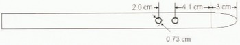
Fig. 11. 2 cm diameter velocity probe. Avalanche flow from right to left.

Shown in Figure 12 are the measurements of depth, normal stress, shear stress, dynamic-friction coefficient and velocity made during this avalanche. The sharp peak shown at t = 0.6 S for the depth gauge is the foot of the gauge bouncing into the air when the second wave of the avalanche hits the foot at 0.4 s. Later, at the tail of the avalanche, snow chunks can be seen going slowly by the depth gauge from t = 5 to 7 s. Using an average snow density of300 kg m ⁻³, the normal stress and depth gauge track each other closely until near the end of the avalanche. From about 0.4 s onward, the optical sensors show a deposit of about 10 cm of stationary snow on the shear box. The ratio of the shear-to-normal stress (S/N =0.42) during the main part of the flow from t = 1 to 3 s is found to be less than the tangent of the slope angle (0.57) in front of the shed, even when the normal stress is reduced by the ∼ 10 cm of stationary snow residing on the plate. The result is accelerating flow as seen by the velocity measurement. As the avalanche comes to rest, the normal stress does not decrease to the static level that would be expected from the 15 cm of deposited snow left at the end of the avalanche. In addition the shear-to-normal stress ratio does not approach the slope angle as it should for an unsupported column of snow. Support for the snow on the shear box is provided by surrounding snow in such a way that the normal stress reading is almost twice what it should be. If the normal stress is reduced to the value for 15 cm of 300 kg m ⁻³ snow on a 30° slope (N = 0.4 kPa) the shear-to-normal stress ends up being 0.6 which works out close to the tangent of the slope angle in front of the shed.

Fig. 12. Depth, normal and shear stress, stress ratio, and velocity for the avalanche of 30 March 1996.

Conclusions

Revolving Door has evolved into an avalanche-test facility where instrumentation has been developed to measure velocity, density, depth, shear and normal stress in a moving avalanche. Several tests have been accomplished but none where all the instrumentation has been operating at the same time. It remains to collect data on avalanches in various types of conditions in order to determine as much information as possible for use in constructing models of avalanche motion. Also, additional instrumentation is being developed to measure air pressure and velocity in the powder cloud or air blast that accompanies the avalanche. Temperature measurements in the flow are planned as well as the use of load cells to measure pressure distribution against various obstacles.