


1. Introduction
Thermoacoustic oscillations arise from the coupling of an unsteady heating process with the acoustic modes of an enclosure (Rayleigh Reference Rayleigh1878). This phenomenon can be found in a variety of technical systems, and it has been a particularly plaguing challenge for the development of modern low-emission gas turbine combustors (Keller Reference Keller1995; Dowling Reference Dowling1997; Candel Reference Candel2002; Lieuwen & Yang Reference Lieuwen and Yang2005; Poinsot Reference Poinsot2017). The vast majority of gas turbine combustors are equipped with annular or can-annular combustor architectures. These systems nominally feature a high degree of spatial symmetry, which leads to interesting properties in the thermoacoustic mode structure, most notably, the occurrence of degenerate mode pairs (Noiray & Schuermans Reference Noiray and Schuermans2013; Bauerheim, Nicoud & Poinsot Reference Bauerheim, Nicoud and Poinsot2016; Magri, Bauerheim & Juniper Reference Magri, Bauerheim and Juniper2016; Mensah et al. Reference Mensah, Magri, Orchini and Moeck2018). The linear modal structure of annular (Noiray, Bothien & Schuermans Reference Noiray, Bothien and Schuermans2011) and can-annular (Ghirardo et al. Reference Ghirardo, Giovine, Moeck and Bothien2019) thermoacoustic systems has been scrutinised to some extent in the past, and can, in fact, be considered as relatively well understood.
In the present work, we explore nonlinear thermoacoustic phenomena in can-annular systems. For this purpose, we conduct a weakly nonlinear analysis of a generic can-annular configuration using the method of averaging. A thorough understanding of the linear modal structure of can-annular systems is a prerequisite; therefore, a concise summary of the relevant elements is given next.
1.1. Linear structure of thermoacoustic modes in can-annular combustors
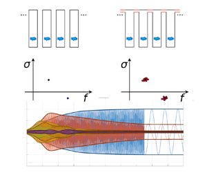
The spectrum of a can-annular system is characterised by the existence of clusters of eigenvalues that form in the vicinity of the thermoacoustic eigenfrequencies of a single isolated can, i.e. in the absence of coupling between the cans (Bethke et al. Reference Bethke, Krebs, Flohr and Prade2002; Panek, Farisco & Huth Reference Panek, Farisco and Huth2017; Ghirardo et al. Reference Ghirardo, Giovine, Moeck and Bothien2019; von Saldern, Orchini & Moeck Reference von Saldern, Orchini and Moeck2021c), as illustrated in figure 1. These mode clusters are linked to the weak coupling between nominally identical cans – the weaker the coupling, the closer the modes are in frequency and growth rate. On a conceptual level, it is straightforward to see that a system consisting of weakly coupled identical subsystems features mode clusters. Let us consider a system of  $N$ identical combustor cans, initially uncoupled (figure 1a,c). In the composite system, each eigenvalue associated with an isolated can appears $N$ times, and because the cans are all identical, these eigenvalues are the same. They are, therefore, (at least) $N$-fold degenerate. In general, this degeneracy will be semisimple since the states in the individual cans are independent and, hence, span the full eigenspace. If we now introduce a weak coupling between adjacent cans (figure 1b,d), this $N$-fold degeneracy is unfold. Since the coupling is weak and the sensitivity of the eigenvalues is bounded, all of the $N$ eigenvalues will be located in the vicinity of the initial $N$-fold degenerate eigenvalue associated with an isolated can. In other words, they form a cluster.

Figure 1. Spectrum of can-annular systems. Qualitative depiction of the emergence of eigenvalue clusters through the weak coupling of identical subsystems. (a,c) Set of  $N$ identical, uncoupled cans. Each eigenvalue of the composite system is $N$-fold degenerate (two are shown, one in the stable and one in the unstable half-plane). (b,d) Set of $N$ identical, weakly coupled cans. The eigenvalues form clusters around the eigenvalues of the uncoupled cans, which leads to the existence of many closely spaced unstable eigenvalues, a feature of can-annular combustors.
Not all of the  $N$ unfold eigenvalues in the weakly coupled system will be distinct. Because of the discrete rotational symmetry of the system, most of the eigenvalues will be two-fold degenerate, more precisely, all except for those with azimuthal orders $0$ and $N/2$ (Ghirardo et al. Reference Ghirardo, Giovine, Moeck and Bothien2019; von Saldern et al. Reference von Saldern, Orchini and Moeck2021c). Here, we assume that $N$ is even, which is the technically relevant case. When $N$ is odd, all modes except those with azimuthal orders being 0 or multiples of $N$ are degenerate. In summary, the composite system consisting of $N$ identical uncoupled cans features $N$-fold degenerate eigenvalues, with algebraic and geometric multiplicity $N$. When a weak coupling between the cans is introduced, the $N$-fold degenerate eigenvalues split into a cluster consisting of two simple eigenvalues and $N/2-1$ degenerate eigenvalues with algebraic and geometric multiplicity two. The existence of eigenvalue clusters, featuring modes with similar frequencies and growth rates, is, hence, a general feature of can-annular thermoacoustic systems. This is in contrast to most of the literature in thermoacoustics, which considers a single unstable mode or a pair of degenerate unstable modes. When many modes are simultaneously unstable, it is not straightforward to predict the final oscillatory state; sophisticated nonlinear analysis techniques have to be utilised. Moreover, such a scenario provides ample opportunity for non-trivial nonlinear phenomena, in particular, synchronisation between modes that are close in frequency and growth rate (von Saldern, Moeck & Orchini Reference von Saldern, Moeck and Orchini2021a). This is further elaborated on in the next section.
1.2. Nonlinear effects and synchronisation
Synchronisation generally refers to the emergence of phase coherence between oscillatory states. This phenomenon has been identified in an abundance of physical, chemical and biological systems since Huygens’ observations of the synchronisation of pendulum clocks. More recently, it has been reported on in thermoacoustic systems in a number of studies. To put the present work into proper context, it is important to acknowledge that a crucial aspect is what states are considered to synchronise. Various forms of synchronisation have been considered in thermoacoustic systems, including phase-locking of an oscillatory state to an external forcing (e.g. Kashinath, Li & Juniper Reference Kashinath, Li and Juniper2018; Guan et al. Reference Guan, Gupta, Wan and Li2019), or the synchronous oscillation of fields (e.g. Pawar et al. Reference Pawar, Seshadri, Unni and Sujith2017; Mondal, Pawar & Sujith Reference Mondal, Pawar and Sujith2018). However, these studies are not directly relevant for the synchronisation of self-excited modes that we consider in the present work. To this extent, we would like to recall some basic facts about synchronisation from the seminal book by Pikovsky, Rosenblum & Kurths (Reference Pikovsky, Rosenblum and Kurths2001).
The relevant setting in the present context is the mutual synchronisation of self-sustained oscillators (Pikovsky et al. Reference Pikovsky, Rosenblum and Kurths2001, see Chap. 4). As highlighted by Pikovsky et al. (Reference Pikovsky, Rosenblum and Kurths2001), synchronisation is only a meaningful concept when the oscillators are self-sustained (possibly self-excited) and if they are weakly coupled. To understand why the first condition is required for synchronisation, consider two oscillators, only one of which is self-excited, with the other being stable. When these are now coupled, even if only weakly, the stable oscillator will always follow the self-excited one. This is not an example of synchronisation, but of response to a forcing. To understand the second condition, consider a scenario in which the coupling is strong. Then, one oscillatory state will always leave a significant trace in the other states it is coupled to. Again, these states share some phase coherence, however, not through a process of synchronisation, merely by virtue of strong coupling. Generally, synchronisation between oscillatory states is favoured through proximity of resonance frequencies. As the resonance frequencies drift apart, an increased level (nonetheless weak) of coupling is required to achieve synchronisation, a phenomenon often represented in the form of Arnold tongues (Pikovsky et al. Reference Pikovsky, Rosenblum and Kurths2001; Balanov et al. Reference Balanov, Janson, Postnov and Sosnovtseva2009). Also note that synchronisation can occur when the oscillation frequency of one state is close to a multiple (harmonic) or fractional multiple (subharmonic) of the resonance frequency of another state.
Now considering a thermoacoustic can-annular system, there are two possible choices for what to consider as states/oscillators when studying synchronisation.
(I) Since the cans are typically weakly coupled, one can consider the thermoacoustic modes of the individual uncoupled cans as oscillatory states that may synchronise under the effect of the coupling. The coupling between adjacent cans is of acoustic or aeroacoustic nature and has reactive and diffusive components; it is linear at leading order but may exhibit finite-amplitude effects (Pedergnana et al. Reference Pedergnana, Bourquard, Faure-Beaulieu and Noiray2021). Chen et al. (Reference Chen, Li, Tang and Yu2021) and Guan et al. (Reference Guan, Moon, Kim and Li2021) reported mutual synchronisation of two coupled, nominally identical thermoacoustic oscillators. In the former study, synchronisation was assessed in a numerical model under variation of the resonator length (frequency detuning) and resonator outlet proximity (coupling strength). Phase-coupled solutions were found to be more likely when frequency detuning is small and the coupling strength large, consistent with basic synchronisation theory. Guan et al. (Reference Guan, Moon, Kim and Li2021) observed similar phenomena experimentally and were able to produce some of them with a low-order model based on coupled van-der-Pol oscillators. Moon et al. (Reference Moon, Guan, Li and Kim2020a) investigated synchronisation between two nominally identical turbulent combustors, acoustically communicating via an adjustable cross-talk gap. When the combustors were operated at identical conditions, in-phase and phase-opposition synchronised states occurred sporadically in a competitive manner, with asynchronous states existing at low coupling strength. Guan et al. (Reference Guan, Moon, Kim and Li2022) consider a system composed of four thermoacoustic oscillators and identify synchronisation and other nonlinear phenomena in symmetric and asymmetric settings.
(II) Alternatively, one can consider the thermoacoustic modes of the full can-annular system as global oscillatory states that may synchronise. In a symmetric setting, these modes will be of Bloch type (Mensah, Campa & Moeck Reference Mensah, Campa and Moeck2016; von Saldern et al. Reference von Saldern, Orchini and Moeck2021c). Furthermore, since the thermoacoustic modes of the full system are biorthogonal, they are linearly uncoupled. They are coupled only through the nonlinear terms in the flame response (and possibly in the can-to-can coupling). As such, this coupling can also be considered weak.
Let us consider the differences between the two settings introduced above. We assume here that the can-annular system features discrete rotational symmetry of the order of the number of cans,  $N$. This implies that all cans, as well as the coupling between them, are identical. In this case, all the states in approach (I) have nominally the same frequencies and growth rates. Because of the direct (linear) coupling and identical eigenfrequencies, synchronised (in the sense of phase-locked) oscillations among the cans are strongly favoured. We can therefore consider that this approach is perhaps more appropriate in an asymmetric case, when the uncoupled cans have slightly different resonance frequencies. On the other hand, the oscillatory states considered in approach (II) will generally have different resonance frequencies. Yet, when the can-to-can coupling is weak, these differences will be small, as explained in § 1.1. Synchronisation is then a possible scenario, but it is challenging to predict under what conditions it occurs and which modes will be involved.
Another point to consider is that approach (II) can be adopted for studying synchronisation phenomena in annular or essentially longitudinal thermoacoustic systems too. Approach (I), on the other hand, would be unsuitable in this context. This is because the individual flames in an annular or sequential combustor cannot be considered as oscillators (assuming that there are no unstable intrinsic thermoacoustic modes). Note, in any case, that synchronisation of thermoacoustic modes in an annular or longitudinal combustor is generally much less likely because the modes are typically not close in frequency. However, it can occur in special circumstances, one example being the manifestation of the slanted mode (Bourgouin et al. Reference Bourgouin, Durox, Moeck, Schuller and Candel2015; Moeck et al. Reference Moeck, Durox, Schuller and Candel2019), which results from the synchronisation of an azimuthal and an axisymmetric thermoacoustic mode. Synchronisation between two longitudinal modes with one having approximately twice the frequency of the other was observed in a sequential combustion system and successfully modelled based on two coupled stochastic oscillators (Bonciolini & Noiray Reference Bonciolini and Noiray2019). Acharya, Bothien & Lieuwen (Reference Acharya, Bothien and Lieuwen2018) investigated the nonlinear interaction of two thermoacoustic modes with close eigenfrequencies based on an oscillator model derived from the Euler equations using a Galerkin expansion. In the present work we will also adopt approach (II) and consider synchronisation between thermoacoustic modes of the full system.
The evolution of the dynamics of a combustor with multiple linearly unstable eigenvalues is governed by the nonlinear modal coupling between the unstable modes. There exist in the literature studies that have focused on assessing this interplay for specific scenarios, with few (two or three) linearly unstable modes. In particular, by using the method of averaging, Noiray et al. (Reference Noiray, Bothien and Schuermans2011) showed how a single pair of degenerate azimuthal modes in an annular configuration saturated by a cubic nonlinearity always converges to spinning solutions; asymmetries are required to stabilise standing azimuthal wave solutions (Noiray & Schuermans Reference Noiray and Schuermans2013). In more recent work, these results have been extended to account also for the effect of noise on the dynamics, showing that (combustion) noise tends to promote the existence of mixed modes (Faure-Beaulieu et al. Reference Faure-Beaulieu, Indlekofer, Dawson and Noiray2021). Instead, Moeck & Paschereit (Reference Moeck and Paschereit2012), Orchini & Juniper (Reference Orchini and Juniper2016) and Acharya et al. (Reference Acharya, Bothien and Lieuwen2018) considered the coexistence of two non-degenerate unstable modes, and derived equations for the (slow) evolution of the oscillation amplitudes, accounting for the modal interaction, using the describing function method or a two time scales approach. They discussed how these equations are able to predict the existence of periodic solutions, in which one of the modes dominates over the other, or quasiperiodic solutions, in which both modes participate in the steady-state oscillations. One significant challenge in these types of analysis is that predicting the existence and stability of multimode solutions requires rather detailed knowledge of the nonlinear terms in the system – a single-input describing function is not sufficient. Moeck et al. (Reference Moeck, Durox, Schuller and Candel2019) considered the nonlinear interaction of three simultaneously unstable modes in an annular combustor, specifically an axisymmetric mode and a pair of degenerate azimuthal modes. This picture becomes significantly more complicated for can-annular systems, because (at least)  $N$ modes – some of which are degenerate – need to be retained in a nonlinear analysis, and their coupling accounted for. Unfortunately, the large number of nonlinear terms that arise in the study of a can-annular system inhibits an analytical analysis of the solutions and their stability.
1.3. Scope
This work aims at developing a weakly nonlinear framework for describing the nonlinear dynamics of can-annular thermoacoustic systems, which are characterised by the presence of clusters of linearly unstable modes. In § 2 we derive from first principles the nonlinear equations that govern the coupled dynamics in the configuration considered. The linear properties of the equations are discussed in § 3, and explicit expressions for the growth rates and frequencies of the eigenvalues as a function of the geometrical and coupling parameters are derived. In § 4 we employ the method of averaging to derive equations for the slow-dynamics of the system. These nonlinear, coupled equations govern the evolution of the amplitudes and frequencies of all the modes that contribute to the oscillations. Lastly, in § 5 we numerically verify the validity of the derived equations, and we use them to discuss what dynamical solutions are supported by can-annular systems, with a focus on the existence of synchronised states in these configurations.
2. Nonlinear time-domain equations for the dynamics of thermoacoustic modes in can-annular systems
We consider a can-annular system composed of  $N$ identical combustor cans coupled to their neighbours at the downstream end by small apertures, which allow for acoustic communication between neighbouring cans. Each can hosts an acoustically compact heat source. The cans form a periodic array, with the $N$th can connected to the first. The geometry is shown schematically in figure 2. The thermoacoustic response of each can, labelled by the index $j$, is described by the conservation of mass, momentum and energy. For the purpose of this study, mean flow effects in the cans are neglected by invoking a low Mach-number assumption (Culick Reference Culick2006). The linearised equations for the conservation of mass, momentum and energy, respectively, read
 $$\begin{gather} \frac{\partial \rho'_j}{\partial t} + \bar{\rho}\boldsymbol{\nabla}\boldsymbol{\cdot} \boldsymbol{u}'_j = 0, \end{gather}$$
 $$\begin{gather}\frac{\partial \boldsymbol{u}'_j}{\partial t} + \frac{1}{\bar{\rho}} \boldsymbol{\nabla} p'_j = 0, \end{gather}$$
 $$\begin{gather}\frac{\partial p'_j}{\partial t} - \bar{c}^2 \frac{\partial \rho'_j}{\partial t} = (\gamma-1)\dot{q}'_j, \end{gather}$$
where  $\boldsymbol {u}' \equiv [u'_x,u'_y,u'_z]$ is the acoustic velocity field, $\bar {\rho }$ the mean density, $p'$ the unsteady pressure fluctuation, $\bar {c}$ the speed of sound (assumed constant), $\gamma$ the heat capacity ratio, and $\dot {q}'$ the unsteady heat release rate due to combustion in a small, acoustically compact volume. These equations may be combined to obtain a second-order partial differential equation for the acoustic pressure fluctuations
 \begin{equation} \frac{\partial^2 p'_j}{\partial t^2} - \bar c^2 \nabla^2 p'_j = (\gamma-1)\frac{\partial \dot{q}'_j}{\partial t}, \end{equation}
which is a wave equation with a source term on the right-hand side, due to the generation of acoustic waves by the unsteady heat release rate. Once a model for  $\dot {q}'$ and boundary conditions are provided, the thermoacoustic equation (2.2) can be solved.

Figure 2. Schematic of the can-annular geometry considered in this study. (a) Top view of the  $N$ connected cans, with depth $H$ and width $B$ in the azimuthal direction $\theta$. (b) Unwrapped side view of the geometry. The cans have height $L$, contain unsteady heat release rate sources $q'$ and are connected by a downstream aperture of axial extension $l_g$. This gap allows for acoustic communication with the neighbouring cans. Note that the azimuthal angle $\theta$ corresponds to the Cartesian $y$ coordinate in the unwrapped representation.
2.1. Coupling between cans
When the cans are connected through small apertures, one needs to account for the acoustic communication from a can to the neighbouring ones. From a can perspective, this can be taken into account as an acoustic mass source/sink along the extension of the aperture (Fournier et al. Reference Fournier, Meindl, Silva, Ghirardo, Bothien and Polifke2021; von Saldern et al. Reference von Saldern, Orchini and Moeck2021c). The aperture is assumed to have surface area  $A_g \equiv l_g H$, where $l_g$ is the axial extension of the apertures and $H$ their depth. By denoting with $\varOmega _{j,j+1}$ the surface of the aperture that allows for acoustic communication between cans $j$ and can $j+1$, a uniform azimuthal transverse velocity is assumed to be present in the aperture
 \begin{equation} u'_{y,j}(\boldsymbol{x},t) = \left\{ \begin{array}{@{}ll} u'_{j,j+1}(t) & \mbox{if } \boldsymbol{x} \in \varOmega_{j,j+1}, \\ 0 & \mbox{otherwise.} \end{array} \right. \end{equation}
 The characteristic frequency of the cluster we are interested in modelling is assumed to be below the cut-on frequency of transverse oscillations in a can, which depends on the speed of sound and the transverse dimensions of the can (Rienstra & Hirschberg Reference Rienstra and Hirschberg2004). Typical cut-on frequencies for transverse modes in realistic configurations are of the order of a few kilohertz. When transverse oscillations are cut off, the acoustics in each can is well-approximated by planar wave propagation along the axial direction  $x$ (Rienstra & Hirschberg Reference Rienstra and Hirschberg2004). While it is true that near the connection between the cans and the gap a non-planar near field exists, as highlighted in Ghirardo et al. (Reference Ghirardo, Giovine, Moeck and Bothien2019), non-planar waves rapidly decay for frequencies below the lowest transverse mode cut-on frequency. The depiction of the acoustics established here is analogous to that of conventional T-junctions used, e.g. to represent the acoustics at the interface of a duct and a transversally mounted Helmholtz resonator (Bothien & Wassmer Reference Bothien and Wassmer2015). By considering frequencies for which all transverse modes are cut off, we can integrate the conservation equations (2.1) over the cross-section of the can, $A_c\equiv BH$, where $B$ is the width of a can. For the conservation of mass (2.1a) this reads
 \begin{equation} \int_0^B {{\rm d}y} \int_0^H {\rm d}z \left[\frac{\partial \rho'_j}{\partial t} + \bar{\rho} \frac{\partial u'_{x,j}}{\partial x} + \bar{\rho} \frac{\partial u'_{y,j}}{\partial y} + \bar{\rho} \frac{\partial u'_{z,j}}{\partial z}\right] = 0. \end{equation}
Furthermore, under the planar wave assumption the acoustic variables are only functions of  $x$, the axial coordinate, and (2.4) simplifies to
 \begin{align} &A_c\left[ \frac{\partial \rho'_j}{\partial t} + \bar{\rho} \frac{\partial u'_{x,j}}{\partial x}\right] + \bar{\rho} H \left[u'_{y,j}(\kern0.7pt y=B) - u'_{y,j}(\kern0.7pt y=0)\right]\varTheta_g(x) \nonumber\\ &\quad + \bar{\rho}B \left[ u'_{z,j}(z=H) - u'_{z,j}(z=0) \right]= 0. \end{align}
 In (2.5),  $u'_{y,j}(\kern0.7pt y=B)$ is the transverse acoustic velocity on the boundary separating cans $j$ and $j+1$, and $u'_{y,j}(\kern0.7pt y=0)$ that on the boundary separating cans $j-1$ and $j$. These are non-zero only along the extension of the aperture, as per (2.3), which is accounted for by introducing the Heaviside function $\varTheta (x)$ and by defining
 \begin{equation} \varTheta_g(x) = \varTheta(x-x_g)\varTheta(x_g+l_g-x), \end{equation}
where  $x_g$ is the upstream end of the aperture. Furthermore, $u'_{z,j} = 0$ at $z=0$ and $z=H$ because of the presence of physical walls, at which the velocity vanishes. To ease the notation, from now onward we will drop the subscript $_x$ from the axial component of the velocity in the cans. Also note that the gap between two combustor cans occupies zero volume in our model, which essentially means that it is assumed acoustically compact.
By integrating also the momentum and energy equations, the conservation laws read
 $$\begin{gather} \frac{\partial \rho'_j}{\partial t} + \bar{\rho} \frac{\partial u'_j}{\partial x} = \bar{\rho} \frac{H}{A_c} \left[u'_{j-1,j} - u'_{j,j+1} \right] \varTheta_g(x), \end{gather}$$
 $$\begin{gather}\frac{\partial u'_j}{\partial t} + \frac{1}{\bar{\rho}}\frac{\partial p'_j}{\partial x} = 0, \end{gather}$$
 $$\begin{gather}\frac{\partial p'_j}{\partial t} - \bar{c}^2 \frac{\partial \rho'_j}{\partial t} = (\gamma-1)\dot{q}'_j. \end{gather}$$
In the absence of transverse acoustic fluctuations ( $u'_{j,j+1} = u'_{j-1,j} = 0$), these equations reduce to the classic one-dimensional thermoacoustic equations in a duct. To obtain a Helmholtz-like equation analogous to (2.2) that accounts for the presence of transverse acoustic fluctuations between the cans, we substitute the conservation of mass (2.7a) into the conservation of energy (2.7c),
 \begin{equation} \frac{\partial p'_j}{\partial t} + \bar{\rho} \bar{c}^2 \frac{\partial u'_j}{\partial x} = \bar{\rho} \bar{c}^2 \frac{H}{A_c} \left[u'_{j-1,j} - u'_{j,j+1}\right] \varTheta_g(x) + (\gamma-1)\dot{q}'_j, \end{equation}
and then combine the latter with the conservation of momentum to obtain a second-order partial differential equation for the acoustic pressure, in which a linear damping term with damping coefficient  $\alpha$ is included (Noiray et al. Reference Noiray, Bothien and Schuermans2011):
 \begin{equation} \frac{\partial^2 p'_j}{\partial t^2} + \alpha\frac{\partial p'_j}{\partial t} - \bar{c}^2 \frac{\partial^2 p'_j}{\partial x^2} = \bar{\rho} \bar{c}^2 \frac{H}{A_c} \left[\frac{\partial u'_{j-1,j}}{\partial t} - \frac{\partial u'_{j,j+1}}{\partial t}\right] \varTheta_g(x) + (\gamma-1)\frac{\partial \dot{q}'_j}{\partial t}. \end{equation}
The structure of the thermoacoustic equation (2.9) for can-annular systems makes it clear how the dynamics in each can is driven by two sources: the classic volumetric energy addition given by the heat release rate  $\dot {q}'$ in that can, and the can-annular-specific acoustic fluctuations at the connections with the neighbouring cans.
2.2. Closure of the equations
To close (2.9) we need to express the source terms, viz. heat release rate and transverse acoustic velocity fluctuations, as functions of the pressure variables. For the heat release rate, we shall employ the simple but widely used cubic saturation relation between the unsteady heat release and the pressure fluctuations, by defining (Noiray et al. Reference Noiray, Bothien and Schuermans2011; Ghirardo, Juniper & Bothien Reference Ghirardo, Juniper and Bothien2018)
 \begin{equation} \dot{q}_j'(x,t) \equiv \left[\beta p_j'(x,t) - \kappa p_j'(x,t)^3 \right]\delta(x_f), \end{equation}
where  $\delta (x)$ denotes Dirac's delta. Flames utilised in gas turbine combustors are typically velocity sensitive; however, the pressure and velocity fluctuations at the flame are directly related through the upstream can impedance. In principle, the combustor cans may communicate with their neighbours through the upstream plenum, but this is usually considered of less importance compared with the cross-talk gap at the turbine inlet (Ghirardo et al. Reference Ghirardo, Giovine, Moeck and Bothien2019).
The acoustic communication between the cans is present only when the pressure difference between neighbouring cans is non-zero, which in turn causes transverse acoustic velocity fluctuations through the gaps. These can then be linked to the pressure difference between two cans by an impedance  $\zeta$, sometimes expressed in terms of the Rayleigh conductivity $K_R$ (Howe Reference Howe1997):
 \begin{equation} \frac{\hat{p}_{j}-\hat{p}_{j+1}}{\hat{u}_{j,j+1}} = \bar{\rho} \bar{c} \zeta, \quad \zeta = \frac{s A_g}{\bar{c} K_R}. \end{equation}
The latter equation is expressed in the frequency domain, for which we adopt the convention  $p'(x,t) \rightarrow \hat {p}(x) {\rm e}^{st}$, with $s\equiv \sigma + \mathrm {i} \omega$, $\sigma$ denoting the growth rate and $\omega$ the angular frequency.
By considering (2.11a,b) also for the pressure difference between can  $j$ and $j-1$, one can express the transverse acoustic velocity fluctuations as a function of the acoustic pressure fluctuations in neighbouring cans as (von Saldern et al. Reference von Saldern, Orchini and Moeck2021c)
 \begin{equation} \hat{u}_{j-1,j} - \hat{u}_{j,j+1} = \frac{1}{{\bar{\rho} \bar{c}}} \frac{1}{\zeta} \left( \hat{p}_{j-1}-2\hat{p}_{j}+\hat{p}_{j+1} \right). \end{equation}
The latter relation is valid at the connection between the cans and the annular section,  $x=x_g$, and should be interpreted as an integral average over the extension of the gap, $l_g$, for an acoustically non-compact connection (von Saldern, Orchini & Moeck Reference von Saldern, Orchini and Moeck2021b).
In the present study, we consider the Rayleigh conductivity to be a complex-valued constant. This is a fair approximation when the analysis is restricted to the vicinity of a frequency  $s = \mathrm {i}\omega _0$ of interest, which corresponds to the frequency at which the cluster of eigenvalues investigated in our analysis is found. Following Howe (Reference Howe1997) (note that due to a different convention in the definition of the Laplace transform, the Rayleigh conductivity (2.13) is the complex conjugate of that reported by Howe (Reference Howe1997)), we define
 \begin{equation} K_R\equiv 2 r_g(\varGamma+\mathrm{i}\varDelta), \end{equation}
where  $r_g \equiv \sqrt {A_g/{\rm \pi} }$ is a characteristic length (equivalent radius) of the aperture. The real part of the Rayleigh conductivity represents a stiffness term, and, when $s=\mathrm {i}\omega _0$, corresponds to the imaginary part of $\zeta$, the can-to-can reactance. Similarly, the imaginary part of $K_R$ represents a damping term, and it corresponds to the real part of the impedance $\zeta$, the can-to-can resistance.
By substituting the expression for the Rayleigh conductivity in (2.12), and recalling its relation (2.11a,b) with the can-to-can impedance  $\zeta$, we obtain
 \begin{equation} s\left[\hat{u}_{j-1,j} - \hat{u}_{j,j+1}\right] = 2r_g\frac{\varGamma+\mathrm{i}\varDelta} {\rho A_g} \left( \hat{p}_{j-1}-2\hat{p}_{j}+\hat{p}_{j+1} \right), \end{equation}
which, in the vicinity of the frequency of interest  $s = \mathrm {i}\omega _0$, can be written in the time domain as
 \begin{equation} \frac{\partial}{\partial t}\left[u'_{j-1,j} - u'_{j,j+1}\right] = \frac{2r_g} {\rho A_g} \left[\varGamma + \frac{\varDelta} {\omega_0} \frac{\partial}{\partial t}\right] \left( p'_{j-1}-2p'_{j}+p'_{j+1} \right). \end{equation}
The latter can be substituted in (2.9), leading to a system of coupled wave equations describing the dynamics of the can-annular configuration
 \begin{align} \frac{\partial^2 p'_j}{\partial t^2} + \alpha\frac{\partial p'_j}{\partial t} - \bar{c}^2 \frac{\partial^2 p'_j}{\partial x^2} &= \bar{c}^2 \frac{H2r_g}{A_c A_g} \left[\varGamma + \frac{\varDelta} {\omega_0} \frac{\partial}{\partial t}\right] \left( p'_{j-1}-2p'_{j}+p'_{j+1} \right) \varTheta_g(x)\nonumber\\ &\quad + (\gamma-1)\beta\frac{\partial p'_j}{\partial t}\delta(x_f) - (\gamma-1)\kappa\frac{\partial p'^3_j}{\partial t}\delta(x_f). \end{align}
Equation (2.16) reveals that there exist two coupling mechanisms between neighbouring cans: one proportional to the pressure difference (reactive coupling, proportional to  $\varGamma$) and one proportional to difference in the rate of change of the pressure (diffusive coupling, proportional to $\varDelta$).
2.3. Galerkin projection
To study (2.16), we employ the Galerkin method to project the dynamics onto a set of prescribed can mode shapes. Because we are interested in studying the dynamics in the vicinity of a thermoacoustic eigenvalue, it is reasonable to assume that, in each can, the dynamics is dominated by a single Galerkin mode
 \begin{equation} p_j'(x,t) = \eta_{j}(t)\psi_{j}(x). \end{equation}
The mode shapes  $\psi _{j}(x)$ are prescribed as the passive thermoacoustic modes with frequency $\omega _0$, identified in each single, uncoupled can, and are subject to the normalisation condition
 \begin{equation} \int_0^L |\psi_{j}(x)|^2 \, {{\rm d}x} = 1. \end{equation}
In this study, we shall consider a can-annular set-up with nominal rotational symmetry, so that the Galerkin mode is identical in all cans,  $\psi _{j}(x) = \psi (x)$, as guaranteed by Bloch's theorem (von Saldern et al. Reference von Saldern, Orchini and Moeck2021c).
By substituting the Galerkin ansatz in (2.16), multiplying the equation by  $\psi ^*$, and integrating over $x$, we obtain a set of coupled equations for the amplitudes of the modes:
 \begin{align} \ddot{\eta}_{j} + \omega_0^2 \eta_{j} &= \left((\gamma-1) |\psi(x_f)|^2 \beta - \alpha \right)\dot{\eta}_{j} \nonumber\\ &\quad +\bar{c}^2\frac{H2r_g}{A_g A_c} \int_{x_g}^{x_g+l_g}|\psi(x)|^2 \,\mathrm{d}x \, \varGamma \left[ \left( \eta_{j-1}-\eta_{j}\right)+\left(\eta_{j+1}-\eta_{j} \right) \right]\nonumber\\ &\quad + \bar{c}^2 \frac{H2r_g}{A_c A_g} \int_{x_g}^{x_g+l_g}|\psi(x)|^2 \,\mathrm{d}x \, \frac{\varDelta} {\omega_0} \left[ \left( \dot{\eta}_{j-1}-\dot{\eta}_{j}\right)+\left(\dot{\eta}_{j+1}-\dot{\eta}_{j} \right) \right] +\mathrm{NL}(\eta_j,\dot{\eta}_j). \end{align}
On the left-hand side, we have isolated the oscillatory dynamics of the mode of interest in can  $j$ in the absence of (i) damping, (ii) coupling with the other cans and (iii) heat release rate dynamics. On the right-hand side we distinguish three contributions to the dynamics: (i) a linear damping/driving term, related to the linear flame response, $\beta$, and the acoustic damping, $\alpha$; (ii) two linear coupling terms, one driven by the reactive coupling $\varGamma$, the other driven by the diffusive coupling $\varDelta$; (iii) nonlinear terms ( $\mathrm {NL}$) that couple the dynamics of the modes and, in our model, originate from the cubic saturation of the heat release rate. For the nonlinear cubic saturation of the heat release rate employed in our analysis, the nonlinear term reads
 \begin{equation} \mathrm{NL}(\eta_j,\dot{\eta}_j) ={-} 3 (\gamma-1) |\psi(x_f)|^4 \kappa \eta_j^2 \dot{\eta}_j. \end{equation}
The coefficients  $\varDelta$ and $\varGamma$ of the coupling terms between the oscillators in (2.19) are all identical because we have assumed a perfect rotational symmetry, implying that the coupling type/strength remains constant (uniform) throughout the entire network of oscillators. This symmetry assumption could be nonetheless relaxed, resulting in can-specific coupling terms $\varDelta _j$ and $\varGamma _j$. This asymmetric scenario will, however, not be considered in this study.
We emphasise that, even though the Galerkin modes are identical, the dynamics of the can-annular system is nonetheless described by a total of  $N$ second-order equations, one for the acoustic oscillations in each can. The collective behaviour of the oscillation amplitudes in each can and their phase patterns are, however, related to the dynamics of the global modes of the entire can-annular combustor, as shown in the next section.
3. Linear response
By neglecting the nonlinear terms in (2.19), we investigate the linear stability of the rotationally symmetric, coupled can-annular system. We introduce the scaled parameters
 \begin{equation} \left.\begin{gathered} \tilde{\varGamma}\equiv \bar{c}^2 \frac{H2r_g}{A_cA_g} \int_{x_g}^{x_g+l_g}|\psi(x)|^2 \,\mathrm{d}x \, \frac{\varGamma}{\omega_0},\quad \tilde{\varDelta}\equiv \bar{c}^2 \frac{H2r_g}{A_cA_g} \int_{x_g}^{x_g+l_g}|\psi(x)|^2 \,\mathrm{d}x \, \frac{\varDelta}{\omega_0}, \\ \tilde{\beta}\equiv (\gamma-1) |\psi(x_f)|^2 \beta, \end{gathered}\right\} \end{equation}
so that (2.19) can be written in the more compact form
 \begin{equation} \ddot{\eta}_j + \omega_0^2\eta_j = \left[\tilde{\beta} - \alpha -2\tilde{\varDelta}\right ] \dot{\eta}_j -2 \omega_0\tilde{\varGamma}\eta_j + \omega_0\tilde{\varGamma} \eta_{j-1}+ \tilde{\Delta} \dot{\eta}_{j-1} + \omega_0\tilde{\varGamma}\eta_{j+1} +\tilde{\Delta}\dot{\eta}_{j+1}. \end{equation}
 The set of  $N$ equations for $j=1,\ldots,N$ is cast in state-space form by introducing the state variables $\zeta _j \equiv \dot {\eta }_j$, so that $\dot {\zeta }_j = \ddot {\eta }_j$. By collecting all the state variables in the state vector $\boldsymbol {z} \equiv [\eta _1,\zeta _1,\ldots,\eta _N,\zeta _N]^{\rm T}$, (3.2) can be rewritten in matrix form as
 \begin{equation} \frac{{\rm d}\boldsymbol{z}}{{\rm d}t} =\mathcal{M} \boldsymbol{z}, \end{equation}
where the matrix  $\mathcal {M}$ is block-circulant and has the form
 \begin{equation} \mathcal{M} = \begin{bmatrix} \mathcal{A} & \mathcal{B} & 0 & \ldots & 0 & \mathcal{B} \\ \mathcal{B} & \mathcal{A} & \mathcal{B} & \ldots & 0 & 0 \\ \vdots & \vdots & \vdots & \ddots & \vdots & \vdots \\ 0 & 0 & 0 & \ldots & \mathcal{A} & \mathcal{B} \\ \mathcal{B} & 0 & 0 & \ldots & \mathcal{B} & \mathcal{A} \end{bmatrix} \end{equation}
with
 \begin{equation} \mathcal{A} \equiv \begin{bmatrix} 0 & 1 \\ -\omega_0^2-2\omega_0\tilde{\varGamma} & \tilde{\beta}-\alpha-2\tilde{\varDelta} \end{bmatrix}, \quad \mathcal{B} \equiv \begin{bmatrix} 0 & 0 \\ \omega_0\tilde{\varGamma} & \tilde{\varDelta} \end{bmatrix}. \end{equation}
In the absence of can-to-can coupling ( $\tilde {\varGamma } = 0$ and $\tilde {\varDelta } = 0$ when $r_g=0$), the matrix $\mathcal {B}$ vanishes, and $\mathcal {M}$ becomes block-diagonal. Each block represents the acoustic dynamics in a decoupled can, with natural (undamped) frequency $\omega _0$ and damping coefficient $\alpha -\tilde {\beta }$. In this limit, the matrix has $N$-fold degenerate eigenvalues. This degeneracy manifests in the ambiguity between the phase of the oscillations in the cans: indeed, with no acoustic communication, any arbitrary phase pattern is possible. As we shall see, the coupling between the cans resolves (some of) the degeneracy: only specific phase patterns are allowed, and different oscillation patterns have slightly different frequencies, which leads to the creation of a cluster of eigenvalues.
To calculate the eigenvalues of (3.3), we recall that block-circulant matrices can always be block-diagonalised (Olson et al. Reference Olson, Shaw, Shi, Pierre and Parker2014). This is accomplished by multiplying  $\mathcal {M}$ from the left and from the right by the unitary matrix $\mathcal {E}_N \otimes \mathcal {I}_2$, where $\otimes$ denotes the Kronecker product, $\mathcal {I}_2$ is the two-dimensional identity matrix, and $\mathcal {E}_N$ is the Fourier matrix of size $N$, defined by
 \begin{equation} \mathcal{E}_N \equiv
\frac{1}{\sqrt{N}}\begin{bmatrix}
1 & 1 & 1 & \ldots & 1 \\
1 & w_N & w_N^2 & \ldots & w_N^{N-1} \\
1 & w_N^2 & w_N^4 & \ldots & w_N^{2(N-1)} \\
\vdots & \vdots & \vdots & \ddots & \vdots \\
1 & w_N^{N-1} & w_N^{2(N-1)} & \ldots & w_N^{(N-1)(N-1)} \end{bmatrix},
\end{equation}
\begin{equation} \mathcal{E}_N \equiv
\frac{1}{\sqrt{N}}\begin{bmatrix}
1 & 1 & 1 & \ldots & 1 \\
1 & w_N & w_N^2 & \ldots & w_N^{N-1} \\
1 & w_N^2 & w_N^4 & \ldots & w_N^{2(N-1)} \\
\vdots & \vdots & \vdots & \ddots & \vdots \\
1 & w_N^{N-1} & w_N^{2(N-1)} & \ldots & w_N^{(N-1)(N-1)} \end{bmatrix},
\end{equation}
with  $w_N \equiv {\rm e}^{\mathrm {i}({2{\rm \pi} }/{N})}$. This yields
 \begin{equation} (\mathcal{E}_N \otimes \mathcal{I}_2)^H \mathcal{M} (\mathcal{E}_N \otimes \mathcal{I}_2) = \mathcal{D} = \begin{bmatrix} \mathcal{D}_0 & & & \boldsymbol{0} \\ & \mathcal{D}_1 & & \\ & & \ddots & \\ \boldsymbol{0} & & & \mathcal{D}_{N-1} \end{bmatrix}, \end{equation}
where  $\mathcal {D}$ is a $2N\times 2N$ block-diagonal matrix, whose blocks $\mathcal {D}_{k-1}$ have dimensions $2\times 2$, and are defined by (Olson et al. Reference Olson, Shaw, Shi, Pierre and Parker2014)
 \begin{equation} \mathcal{D}_{k-1} \equiv \mathcal{A} + \mathcal{B}\omega_N^{(k-1)} + \mathcal{B}\omega_N^{(N-1)(k-1)} = \mathcal{A} + 2\mathcal{B}\cos\left(\frac{2{\rm \pi}}{N}(k-1)\right), \quad k = 1,\ldots,N. \end{equation}
By recognising  $k-1$ as the Bloch number $b$, the block matrix $\mathcal {D}_b$ reads
 \begin{align} \mathcal{D}_b = \begin{bmatrix} 0 & 1 \\ -\omega_0^2-4\omega_0\tilde{\varGamma}\sin^2\left(\dfrac{{\rm \pi} b}{N}\right) & \tilde{\beta}-\alpha-4\tilde{\varDelta}\sin^2\left(\dfrac{{\rm \pi} b}{N}\right) \end{bmatrix}, \quad \mbox{for } b = 0,\ldots,N-1, \end{align}
and the dynamics of the  $b$th mode is described by the linear eigenvalue problem
 \begin{equation} \mathcal{D}_b \boldsymbol{v}_b = s_b \boldsymbol{v}_b. \end{equation}
 The growth rate and angular frequency of the eigenvalues  $s_b \equiv \sigma _b + \mathrm {i} \omega _b$ of the matrix $\mathcal {D}_b$, defined in (3.9), are
 $$\begin{gather} \sigma_b = \frac{\tilde{\beta}-\alpha}{2}-2\tilde{\varDelta}\sin^2\left(\frac{{\rm \pi} b}{N}\right), \end{gather}$$
 $$\begin{gather}\omega_b = \sqrt{\omega_0^2 -\left(\frac{\tilde{\beta}-\alpha}{2}\right)^2 + 2\left[\left(\tilde{\beta}-\alpha\right)\tilde{\varDelta}+2\omega_0\tilde{\varGamma} \right]\sin^2\left(\frac{{\rm \pi} b}{N}\right) - 4\tilde{\varDelta}^2 \sin^4\left(\frac{{\rm \pi} b}{N}\right)}. \end{gather}$$
Equations (3.11) are analytical expressions that describe the distribution of all the can-annular eigenvalues in a cluster associated with a single-can mode as a function of the system parameters (nominal frequency, nominal damping and real and imaginary parts of the coupling impedance). The Bloch number  $b$ takes value from 0 to $N-1$, or equivalently from $-N/2+1$ to $N/2$ if $N$ is even, or from $-(N-1)/2$ to $(N-1)/2$ if $N$ is odd. Because $\sin ^2({\rm \pi} b/ N)$ is an even function, it holds that $s_{b} = s_{-b}$, leading to two-fold degeneracy of all modes with $b\neq 0$ and $b\neq N/2$. For $b=0$ the expressions retrieve the eigenvalue of a single, isolated can, given by
 \begin{equation} s_0 = \frac{\tilde{\beta}-\alpha}{2} \pm \mathrm{i}\omega_0\sqrt{1 -\left(\frac{\tilde{\beta}-\alpha}{2\omega_0}\right)^2 }. \end{equation}
 The eigenvectors  $\boldsymbol {z}_b$ of the linear system (3.3) are given by $(\mathcal {E}_N \otimes \mathcal {I}_2) \boldsymbol {v}_b$, where $\boldsymbol {v}_b$ is the $2\times 1$ eigenvector in the block-diagonal formulation. Because of the nature of $(\mathcal {E}_N \otimes \mathcal {I}_2)$, it can be shown (Olson et al. Reference Olson, Shaw, Shi, Pierre and Parker2014) that both the states contained in the eigenvectors $\boldsymbol {z}_b$ follow a discrete Fourier mode pattern of order $b$.
$b$.
4. Weakly nonlinear dynamics
When performing a weakly nonlinear analysis, all the modes that are linearly unstable, and thus can contribute to the dynamics, need to be retained. Due to the formation of eigenvalue clusters in can-annular systems, if the uncoupled eigenvalue  $\omega _0$ is marginally stable, so are all the eigenvalues of the weakly coupled can-annular system – as per (3.11a) when $\tilde {\varDelta }$ is small compared with $(\tilde {\beta } - \alpha )$. All the $N$ modes in this cluster must therefore be retained. In our analysis, it is assumed that a single cluster is (marginally) unstable.
Weakly nonlinear analysis of thermoacoustic oscillations in longitudinal and annular configurations has been conducted previously (Ghirardo, Juniper & Moeck Reference Ghirardo, Juniper and Moeck2016; Orchini, Rigas & Juniper Reference Orchini, Rigas and Juniper2016). In these works, however, the interaction of multiple linearly unstable modes with close but initially unequal frequencies and growth rates, which is the generic setting for can-annular systems, was not considered. Rather than describing the amplitude of the oscillations in each can, it is more appropriate for a nonlinear analysis to describe the amplitude of the global modes. This is because, from the results of the linear analysis in § 3, we know that the can-annular pressure mode shapes in a cluster have the form of Fourier modes with azimuthal order up to  $N/2$. We wish to track the evolution of the amplitude of these physically motivated mode shapes, which exponentially grow in time in the linear regime, and lead to nonlinear modal interactions when the amplitudes reach non-negligible values. Thus, by using the results of the linear analysis, and by recalling that the $y$ direction in figure 2 is equivalent to the azimuthal direction $\theta$, the global pressure dynamics can be described as
 \begin{align} p_j(x,t) = p(x,\theta_j,t) &= \eta_{0c}(t)\psi(x) + \eta_{N/2c}(t)\psi(x)\cos(N/2 \, \theta_j) \nonumber\\ &\quad +\sum_{m=1}^{N/2-1} \left[ \eta_{mc}(t)\psi(x)\cos(m\theta_j) + \eta_{ms}(t)\psi(x)\sin(m\theta_j) \right]. \end{align}
The subscript  $_{mc}$ indicates the mode with structure $\cos (m\theta )$ for $m=0,\ldots,N/2$, whereas $_{ms}$ the mode with structure $\sin (m\theta )$ for $m=1,\ldots,N/2-1$. Note that, from the linear stability results of § 3, we have exploited the fact that the $m=0$ (push–push) and $m=N/2$ (push–pull) are non-degenerate.
Using the ansatz (4.1) in the can-annular Helmholtz equation (2.16), and defining the scaled saturation constant  $\tilde {\kappa } \equiv (\gamma -1) |\psi (x_f)|^4 \kappa$, together with the coefficients (3.1), yields a set of second-order, coupled, nonlinear ordinary differential equations governing the dynamics of each mode:
 \begin{equation} \ddot{\eta}_{mc/s} + \omega_0^2 \eta_{mc/s} = (\tilde{\beta} - \alpha) \dot{\eta}_{mc/s} - 4 \sin^2\left(\frac{m{\rm \pi}}{N}\right) \left(\omega_0\tilde{\varGamma}\eta_{mc/s} + \tilde{\Delta} \dot{\eta}_{mc/s}\right) - 3\tilde{\kappa}\mathcal{N}_{mc/s}, \end{equation}
with  $\mathcal {N}_{mc/s}$ defined by
 \begin{align} \mathcal{N}_{mc} = \frac{1}{(1+\delta_{m0}){\rm \pi}}\int_0^{2{\rm \pi}} \cos(m\theta) \frac{\partial p'}{\partial t} p'^2 \,{\rm d}\theta, \quad \mathcal{N}_{ms} = \frac{1}{\rm \pi}\int_0^{2{\rm \pi}} \sin(m\theta) \frac{\partial p'}{\partial t} p'^2 \,{\rm d}\theta. \end{align}
The Kronecker delta  $\delta _{m0}$ in the normalisation accounts for the fact that all modes with $m\neq 0$ average to ${\rm \pi}$ when integrated over the circumference, whereas the mode with $m=0$ averages to $2{\rm \pi}$. The expressions for $\mathcal {N}$ can be made explicit by means of trigonometric identities, but become very large for increasing values of $N$. For $N=8$ cans, each $\mathcal {N}$ contains over 100 terms. Their explicit expressions are thus not fully reported in the manuscript, but an example calculation of one of these terms is provided in the Appendix A.
Note that the left-hand side is identical for all the modes. This reflects the fact that, in the absence of coupling, the cans are free to oscillate at the same frequency with any circumferential phase pattern. The linear corrections due to the can-to-can coupling to the frequencies (given by the terms proportional to  $\tilde {\varGamma }$) and to the growth rates (given by the terms proportional to $\tilde {\varDelta }$) are considered as perturbations of the undamped oscillators, all sharing the same natural frequency $\omega _0$.
To perform a weakly nonlinear analysis, we write
 \begin{equation} \eta_{mc/s} = A_{mc/s} \cos\left(\omega_0 t + \phi_{mc/s}\right), \quad \dot{\eta}_{mc/s} ={-} \omega_0 A_{mc/s} \sin\left(\omega_0 t + \phi_{mc/s}\right), \end{equation}
where  $A$ and $\phi$ are slowly varying functions of time. Their dynamics can be retrieved by a moving average of the equations over a period $T=2{\rm \pi} /\omega _0$, i.e. an oscillation period of the fast time scale defined by the uncoupled oscillators. The averaged quantities are denoted by an overbar, and are defined by
 \begin{equation} \bar{g}(t) = \langle g\rangle(t) \equiv \frac{1}{T} \int_{t}^{t+T} g(s) \,{\rm d}s. \end{equation}
After rewriting the original equation in standard form,  $\ddot {\eta } + \omega _0^2\eta + h(\eta,\dot {\eta })=0$, first-order, coupled nonlinear ordinary differential equations that govern the (slow) evolution of the amplitudes and phases can be obtained (Strogatz Reference Strogatz1994):
 \begin{equation} \dot{\bar{A}} = \left\langle\frac{ h(A,\phi)}{\omega_0}\sin(\omega_0t+\phi)\right\rangle \quad \mbox{and} \quad \dot{\bar{\phi}} =\left\langle \frac{ h(A,\phi)}{\omega_0 A}\cos(\omega_0t+\phi)\right\rangle. \end{equation}
By approximating the instantaneous values on the right-hand side of (4.6a,b) with the averaged values, the evolution of the amplitudes and phases of (4.2) is given by
 $$\begin{gather} \dot{\bar{A}}_{mc/s} = \frac{\tilde{\beta} - \alpha}{2} \bar{A}_{mc/s} - 2\tilde{\varDelta} \sin^2\left(\frac{m{\rm \pi}}{N}\right) \bar{A}_{mc/s} + 3\tilde{\kappa} \left\langle \frac{\mathcal{N}_{mc/s}}{\omega_0} \sin(\omega_0t + \bar{\phi}_{mc/s}) \right\rangle, \end{gather}$$
 $$\begin{gather}\dot{\bar{\phi}}_{mc/s} = 2\tilde{\varGamma}\sin^2\left(\frac{m {\rm \pi}}{N}\right) + 3\tilde{\kappa}\left\langle \frac{\mathcal{N}_{mc/s}}{\omega_0A_{mc/s}} \cos(\omega_0t + \bar{\phi}_{mc/s}) \right\rangle. \end{gather}$$
In the absence of the nonlinear terms, the amplitudes of the modes grow exponentially, according to the linear term in (4.7a), with the same growth rates as those predicted by (3.11a). The phases of all modes with  $m\neq 0$ drift at a constant rate, indicating a shift in frequency of $2\tilde {\varGamma }\sin ^2(m{\rm \pi} /N)$, as per the constant term in (4.7b). This frequency correction is not identical to that predicted by the linear analysis, as in (3.11b). This result is, however, correct in the limits considered for the method of averaging, in which even the linear deviations from the unperturbed oscillator, proportional to $(\tilde {\beta }-\alpha )$, $\tilde {\varGamma }$ and $\tilde {\varDelta }$, are considered small and expanded to first order. Indeed, a Taylor expansion of (3.11b) around $\omega _0$ retrieves, at first order, the same frequency shift as the method of averaging. Higher-order corrections to the frequency can be retrieved by the method of averaging by considering higher-order terms when averaging the equations. However, since the frequency drift is generally small, these higher-order effects will not be considered in this study.
5. Results and discussion
In this section we present and discuss results obtained by integrating the slow dynamics equations for the evolution of the amplitude and the phase of an  $N=8$ can-annular configuration. Although the equations derived in §§ 3 and 4 are valid for an arbitrary number $N$ of cans, in order to present quantitative results, we need to fix $N$ to a specific value. In general, it should be expected that the results will depend on the specific value of $N$, since, as $N$ increases, qualitatively different types of solutions exist. The specific value $N=8$ was chosen to balance the complexity of the dynamics to the manageability of the nonlinear terms in the equations. The configuration considered here models the atmospheric can-annular experimental set-up assembled at the Norwegian University of Science and Technology and described by Buschmann, Worth & Moeck (Reference Buschmann, Worth and Moeck2023). We refer to the latter for details about the geometry. For all the calculations in the following, we have set $(\tilde {\beta } - \alpha )/2 \approx 23\ {\rm s}^{-1}$, $\omega _0 \approx 2{\rm \pi} \times 180\ {\rm rad}\ {\rm s}^{-1}$ and $\tilde {\kappa } \approx 50$, and varied the strength of the (aero)acoustic coupling between the cans by varying $\tilde {\varDelta }$ and $\tilde {\varGamma }$. The value of the driving $(\tilde {\beta }- \alpha )$ term was chosen to be approximately 2 % that of $\omega _0$ because (i) the method of averaging requires $(\tilde {\beta } - \alpha ) \ll \omega _0$ to yield accurate results at first order and (ii) it was observed that the magnitude of this value is consistent with typical positive growth rates found in Orchini et al. (Reference Orchini, Pedergnana, Buschmann, Moeck and Noiray2022), where the same experimental set-up of Buschmann et al. (Reference Buschmann, Worth and Moeck2023) was modelled. The nonlinear saturation coefficient $\kappa$ was instead tuned in order to have oscillation amplitudes with a maximum value close to unity.
5.1. Fast and slow dynamics
To validate the method of averaging presented in § 4, we integrate numerically both the fast evolution of the coupled oscillators, (4.2), and the slow, averaged evolution of the amplitudes and phases of all the linearly unstable modes, (4.7).
Figure 3 shows the evolution of the coefficients  $\eta _{jm}$ with thinner lines; a fast oscillation is apparent. To emphasise the oscillating nature of these time series, the last 20 ms, containing approximately three full cycles, are stretched in each panel. With the provided initial conditions, the oscillations converge to a push–push mode ( $b=0$). The decay of the amplitudes of the modes with $m=1,2$ is relatively slow and not visible in the reported data, which show only the evolution of the dynamics for a total time of 1 s. Figure 3 shows also the evolution of the modal amplitudes as predicted by the method of averaging with thicker, darker lines. The initial conditions of the averaged equations are chosen to be identical to those of the oscillator dynamics, by exploiting the relation between the oscillator states and the amplitudes and phases of the modes provided by (4.3a,b) at $t=0$ s. Despite the highly non-monotonic behaviour of the oscillation amplitudes, the evolution of the amplitudes, as approximated by the method of averaging, compares very favourably with the real amplitudes of the oscillators. The averaged solutions can, in fact, also predict the modulation of the oscillation amplitudes, which is due to beating and nonlinear modal interaction, both typical of the transient dynamics of systems with multiple, closely spaced eigenvalues.

Figure 3. Time integration of the fast (thin, lighter colours) and slow (thick, darker colours) dynamics of the considered weakly nonlinear can-annular system. Each panel shows the evolution of the amplitude of one of the  $N=8$ modes that contribute to the dynamics; similar colours denote degenerate modes. Results obtained for $\tilde {\varGamma }=54$ and $\tilde {\varDelta }=0$.
To assess the description of the phase dynamics from the method of averaging, we need to extract phase information from the dynamics of the oscillators. For each real-valued time trace  $\eta _{mj}(t)$, we perform a Hilbert transform to obtain the imaginary part of the complex-valued analytic signal $\mathcal {H}[\eta _{mj}](t)$, which satisfies ${\rm Re}[\mathcal {H}[\eta _{mj}](t)] = \eta _{mj}(t)$. The magnitude, $|\mathcal {H}[\eta _{mj}]|$, and the phase angle, $\varphi _{mj} \equiv \angle (\mathcal {H}[\eta _{mj}])$ of these complex oscillatory signals correspond to the instantaneous amplitude and phase of the dynamics of the oscillator $\eta _{mj}$. The phase $\varphi _{mj}$ contains information on both the natural phase of the uncoupled oscillators, defined by $\phi _0 = \omega _0 t$, and on the deviation from the latter of the coupled, nonlinear system. The method of averaging approximates the latter, and to allow for a comparison, we define
 \begin{equation} \phi_{mj} \equiv \varphi_{mj} - \phi_0 \equiv \angle(\mathcal{H}[\eta_{mj}]) - \omega_0 t. \end{equation}
Figure 4 shows a comparison between the instantaneous phases of the oscillators – solid lines, lighter colours – obtained with the Hilbert transform, and the averaged phases obtained by integrating directly the slow dynamics equations (4.7) – dashed lines, darker colours. Except for some inaccuracy introduced by the finite-length Hilbert transform at the beginning and end of the time series, the comparison between the phases is strikingly good.

Figure 4. Time integration of the fast (solid, lighter colours) and slow (dashed, darker colours) dynamics of the considered weakly nonlinear can-annular system. The time interval shown corresponds to 4 seconds. The panels show the instantaneous phase of the oscillations, defined as a deviation from the natural phase of the uncoupled oscillators,  $\phi _0 = \omega _0 t$. Similar colours refer to degenerate modes. Results obtained for $\tilde {\varGamma }=54$ and $\tilde {\varDelta }=0$.
Although not shown, analogous comparisons have been performed for various values of the coupling parameters  $\tilde {\varDelta }$ and $\tilde {\varGamma }$, and a good match between the averaged and exact oscillator dynamics has always been observed. These results validate the derivation and implementation of the averaged equations, and for this reason in the following sections we will only show and discuss results obtained from the averaged equations.
5.2. Initial conditions and supported solutions
To study which types of solutions the system supports, we rely on the numerical integration of the averaged equations from a variety of initial conditions. In this way, we assess whether specific solutions are supported by the equations. By fixing  $\tilde {\varDelta } = 0$ and $\tilde {\varGamma } = 21$, we alternately set the initial amplitude of one of the modes to one, while setting the amplitudes of the remaining modes to $10^{-5}$. All phases are arbitrarily chosen to start at $\bar {\phi }_{mj}=0$. This particular set of initial conditions is chosen to assess the stability of standing solutions. Because we have chosen a standing basis for decomposing the pressure dynamics in the cans, a pure standing solution is found if, for example, the amplitude of one mode with $0< m< N/2$ is non-zero, and all other amplitudes are zero.
Figure 5 shows the evolution of the amplitudes and phases of all the considered initial conditions. Only the evolution of the phase difference between the modes that participate in the steady-state, stable oscillation are shown for each case. Starting from figure 5(a), initialising the oscillations to a push–push mode results in a stable push–push state (mode 0c). In the steady-state, the phase of this mode is flat, denoting that no frequency drift occurs, and the final steady-state oscillations have the same frequency of the uncoupled system,  $\omega _0$, which is a general characteristic of push–push modes (von Saldern et al. Reference von Saldern, Moeck and Orchini2021a,Reference von Saldern, Orchini and Moeckc). When initialising the oscillations to a standing mode with $m=1$, figure 5(c,d), instead, the nonlinear modal interaction triggers the participation of other modes. After a transient, the amplitudes of all modes drop to zero, except those of the two standing modes with $m=1$, which converge to the same value. In the steady state, their phases exhibit a constant drift, and are shifted apart by ${\rm \pi} /2$. In conjunction with the amplitudes reaching the same level, this indicates that the system has converged to a spinning solution since it holds that
 \begin{align} A\cos(\omega_0 t +\phi(t)) \cos(\theta) + A\cos(\omega_0 t+\phi(t)+{\rm \pi}/2) \sin(\theta) = A \cos(\omega_0 t + \phi(t) + \theta). \end{align}
The slope of the phase in the steady state reaches a value of  $6.15\ {\rm rad}\ {\rm s}^{-1}$ for both modes. This compares very well with the linear correction to the unperturbed angular frequency predicted by the method of averaging, $\Delta \omega \equiv 2\tilde {\varGamma }\sin ^2(m{\rm \pi} /N)$, as per (4.7b).

Figure 5. Evolution of the amplitudes and phases of the coupled dynamics of an  $N=8$ can-annular system when the oscillations are initialised to (a) a push–push mode, (b) a push–pull mode, (c,d) a standing mode with $m=1$, (e,f) a standing mode with $m=2$, (g,h) a standing mode with $m=3$. The coupling parameters are set to $\tilde {\varGamma }=21$ and $\tilde {\varDelta }=0$.
Similar results hold for cases in which standing solutions with  $m=2$, figure 5(e,f), and $m=3$, figure 5(g,h), were initialised. In all these cases, after a transient, the solutions diverge from the initial standing state and converge to spinning modes with order $m$ corresponding to that of the initial standing mode. This result is consistent with the findings of Noiray et al. (Reference Noiray, Bothien and Schuermans2011), where it was shown that standing oscillations are not stable solutions in symmetric annular configurations saturated by a cubic nonlinearity. The angular frequency drifts calculated from the slopes of the phases are $\Delta \omega =21\ {\rm rad}\ {\rm s}^{-1}$ and $\Delta \omega = 35.8\ {\rm rad}\ {\rm s}^{-1}$, for oscillations of spinning modes with $m=2$ and $m=3$, respectively. Once again, these values coincide with those predicted by the linear term in (4.7b).
5.3. Synchronisation
A different behaviour is observed when the solutions are initialised to a push–pull mode (figure 5b). In this case, multiple modes with different values of  $m$ are triggered by the nonlinear modal interaction, and survive in the final, steady-state oscillations. In particular, the $m=4$ push–pull mode, both modes with $m=3$ and one of the modes with $m=2$ participate in the finite-amplitude oscillation. Figure 5 shows only a total integration time of 4 s; at larger times the amplitudes of both standing modes with $m=3$ converge to the same amplitude, $A_{3j} = 0.67$, but with a phase difference of zero. This corresponds to a standing mode, but rotated by ${\rm \pi} /4$ with respect to those used as a basis, and with an amplitude of $\sqrt {2}A_3$. The amplitudes of the modes with $m=2$ and $m=4$ converge to $A_{2s} = 0.24$, $A_{4c} = 0.88$, respectively, and their phases have a constant phase difference with respect to the modes having $m=3$. This is a signature of synchronisation. By synchronisation we mean the adjustment of rhythms of oscillators due to their weak interaction, as defined by Pikovsky et al. (Reference Pikovsky, Rosenblum and Kurths2001). As discussed in § 1.2, two conditions must be satisfied for synchronisation to be possible: (i) the oscillators must be self-sustained when decoupled; and (ii) a weak coupling must be established between the oscillators. By using the results derived in § 3, we can verify that these conditions are easily satisfied for can-annular geometries. When the cans are decoupled, $\tilde {\varGamma } = \tilde {\varDelta } = 0$, the eigenvalues of all the $N$ modes converge to (3.12). Thus, provided that the isolated can system is thermoacoustically unstable, $(\tilde {\beta } - \alpha )>0$, condition (i) is satisfied because there exist a set of $N$ self-sustained oscillation patterns in the system, one in each can. A (weak) coupling between the cans is present when $\tilde {\varGamma } \neq 0$ and/or $\tilde {\varDelta } \neq 0$, satisfying condition (ii). Furthermore, the linear effect of the weak coupling can be quantitatively seen from (3.11). All the growth rates $\sigma _b$ and angular frequencies $\omega _b$ are close to the frequency of an isolated can. If the growth rate of an uncoupled thermoacoustic mode is positive, $(\tilde {\beta }-\alpha )/2 > 0$, then one should expect all the eigenvalues of the coupled can-annular system to have a positive growth rate, because they form a cluster. All these modes grow exponentially in the linear regime and interact with each other during the transient response. The interaction between modes may suppress the growth of some modes and enhance the growth of others. Furthermore, the nonlinear interaction causes a drift of the oscillation frequencies as the amplitude of oscillation increases. Under appropriate conditions, these frequencies may lock to the same value: if modes with different linear oscillation frequencies persist in the saturated oscillation state with the same frequency, synchronisation has occurred.
Identifying explicit conditions for synchronisation is a non-trivial task, because one needs to find synchronised states that are supported by the governing equations (4.7), and verify that these solutions are stable. Already for  $N=8$, this problem is complex to treat analytically because the phase space is 16-dimensional, and there exists a very large number of possible synchronised states. It is, however, analytically treatable for $N=3$. The expressions of the governing equations (4.7) including all the nonlinear terms can be explicitly reported for this case:
 \begin{align} \dot{\bar{A}}_{0c} &= \frac{\tilde{\beta} - \alpha}{2} \bar{A}_{0c} \nonumber\\ &\quad - \frac{3\tilde{\kappa}}{16} \bar{A}_{c0}\left[\bar{A}_{c1}^2 \cos(2\bar{\phi}_{c0}-2\bar{\phi}_{c1})+\bar{A}_{s1}^2 \cos(2\bar{\phi}_{c0}-2\bar{\phi}_{s1})+2\bar{A}_{c0}^2+2\bar{A}_{c1}^2+2\bar{A}_{s1}^2\right], \end{align}
 \begin{align} \dot{\bar{A}}_{1c} &= \frac{\tilde{\beta} - \alpha}{2} \bar{A}_{1c} - 3\tilde{\Delta} \bar{A}_{1c}\nonumber\\ & \quad- \frac{3\tilde{\kappa}}{32}\bar{A}_{c1}\left[4\bar{A}_{c0}^2\cos(2\bar{\phi}_{c0} - 2\bar{\phi}_{c1}) + \bar{A}_{s1}^2\cos(2\bar{\phi}_{c1} - 2\bar{\phi}_{s1}) + 8\bar{A}_{c0}^2 + 3\bar{A}_{c1}^2 + 2\bar{A}_{s1}^2\right], \end{align}
 \begin{align} \dot{\bar{A}}_{1s} &= \frac{\tilde{\beta} - \alpha}{2} \bar{A}_{1s} - 3\tilde{\Delta}\bar{A}_{1s} \nonumber\\ &\quad - \frac{3\tilde{\kappa}}{32} \bar{A}_{s1}\left[4\bar{A}_{c0}^2\cos(2\bar{\phi}_{c0} - 2\bar{\phi}_{s1}) + \bar{A}_{c1}^2\cos(2\bar{\phi}_{c1} - 2\bar{\phi}_{s1}) + 8 \bar{A}_{c0}^2 + 2 \bar{A}_{c1}^2 + 3 \bar{A}_{s1}^2\right], \end{align}
 $$\begin{gather} \dot{\bar{\phi}}_{0c} ={+} \frac{3\tilde{\kappa}}{16} \left[\bar{A}_{c1}^2\sin(2\bar{\phi}_{c0} - 2 \bar{\phi}_{c1}) + \bar{A}_{s1}^2 \sin(2\bar{\phi}_{c0} - 2\bar{\phi}_{s1}) \right], \end{gather}$$
 $$\begin{gather}\dot{\bar{\phi}}_{1c} = 3\tilde{\varGamma}+ \frac{3\tilde{\kappa}}{8} \left[ \frac{\bar{A}_{s1}^2}{4} \sin(2\bar{\phi}_{c1} - 2\bar{\phi}_{s1}) - \bar{A}_{c0}^2\sin(2\bar{\phi}_{c0} - 2\bar{\phi}_{c1})\right], \end{gather}$$
 $$\begin{gather}\dot{\bar{\phi}}_{1s} = 3\tilde{\varGamma}-\frac{ 3\tilde{\kappa}}{8} \left[ \bar{A}_{c0}^2\sin(2\bar{\phi}_{c0} - 2\bar{\phi}_{s1}) + \frac{\bar{A}_{c1}^2}{4}\sin(2\bar{\phi}_{c1} - 2\bar{\phi}_{s1})\right]. \end{gather}$$
One can verify that these equations are equivalent to equation (5) presented by Moeck et al. (Reference Moeck, Durox, Schuller and Candel2019), which were derived to model synchronisation between an axisymmetric and an azimuthal mode in an annular combustor. We note that the physical meaning of the coupling terms is different: the reactive ( $\hat {\varDelta }$) and resistive ( $1-\hat {\sigma }$) coupling terms in the work of Moeck et al. (Reference Moeck, Durox, Schuller and Candel2019) are directly related to differences in the frequencies/growth rates of longitudinal and azimuthal modes in an annular combustion chamber. On the other hand, the reactive ( $\tilde {\varGamma }$) and resistive ( $\tilde {\varDelta }$) terms in the can-annular model presented in this work stem from the Rayleigh conductivity that provides a weak coupling between otherwise identical cans. Although the geometry and the detailed interpretation of the parameters are different, the physics underlying the thermoacoustic phenomenon is the same, and it should not come as a surprise that equations with the same structure appear here.
Given the equivalent representation of the dynamics, we can directly apply the results of Moeck et al. (Reference Moeck, Durox, Schuller and Candel2019) about synchronisation, shown in their figure 3, to the can-annular system considered here: for  $N=3$, synchronisation is possible only for specific combinations of the reactive and resistive coefficients. In particular, we can exploit their result to conclude that, for $N=3$, $\tilde {\varDelta }$ must be negative for synchronisation to occur – the resistance $\tilde {\varDelta }$ is proportional to the parameter ( $1-\hat {\sigma }$) of Moeck et al. (Reference Moeck, Durox, Schuller and Candel2019). An interesting question is whether a negative resistance is a strict requirement for synchronisation in can-annular systems with a larger number of cans, say $N=8$. The extension of this result to a larger number of cans could not formally be proven. Instead, we relied on extensive numerical calculations for the $N=8$ case to investigate when synchronisation occurs. The results suggest that our model supports synchronised solutions only for negative values of the resistivity. It was reported in Pedergnana et al. (Reference Pedergnana, Bourquard, Faure-Beaulieu and Noiray2021) that such a negative resistance may be induced in a frequency band by aeroacoustic effects that excite the shear layer formed by the grazing flow along the can-to-can apertures.
For our calculations, we consider coupling parameters in the range  $\tilde {\varDelta }/(\tilde {\beta }- \alpha ) \in [-0.5,0.5]$ for the resistance and $\tilde {\varGamma }/(\tilde {\beta } - \alpha ) \in [-0.5, 0.25]$ for the reactance. Starting from the smallest values of both coupling parameters, we initialise (4.7) close to the unstable fixed points, with amplitudes equal to $10^{-5}$ and phases randomly distributed in the range $[0,2{\rm \pi} ]$. We integrate the equations until $t=200$ s, to ensure convergence of the results. We then assess if the final state is synchronised by determining how many modes contribute to the final steady-state oscillations (with amplitudes larger than 0.05), and by comparing the slopes of the phases – in other words, the frequencies. Each subsequent calculation is then initialised from the end state of a neighbouring state, following a continuation-like approach. Because the first identified state is synchronised, the approach we follow is able to identify when the stability of synchronised solutions is lost. Figure 6 shows the results by using on the left a colour scheme that assigns a unique colour to states with $n$ synchronised modes, where $n=0$ means that no synchronisation occurs, and on the right the same colour scheme as in figure 3 to show which mode has the largest amplitude in the final, possibly synchronised state. It is observed that synchronised states are stable when $\tilde {\varDelta }<0$, consistent with the analytical findings of Moeck et al. (Reference Moeck, Durox, Schuller and Candel2019) for $N=3$. However, in contrast to the latter study, the window of synchronisation is much larger. This is likely because in that study only one synchronisation pattern was possible, whereas in the can-annular configuration considered in the present work, a large number of possible synchronised states exist. Furthermore, in the identified synchronised states the push–pull ( ${4c}$) mode has the largest amplitude – an example can be seen in figure 5(b). On the other hand, when synchronisation does not happen, for most $\tilde {\varDelta }>0$, the push–push ( $0c$) mode dominates the dynamics. We note that analogous results were reported in Pedergnana & Noiray (Reference Pedergnana and Noiray2022), where dominant push–push oscillations for positive values of the resistive coupling and dominant push–pull oscillations for negative values of the resistive coupling were reported. We, however, also observe that there exist regions of positive resistance where synchronisation persists. We, however, emphasise that these solutions have been obtained by tracking synchronised solutions from negative resistance to positive resistance and that figure 6 provides no information on the basins of attraction of these synchronised solutions, nor on the possible existence of other stable oscillatory states. We also highlight that the synchronised map shown in figure 6 exhibits a clear symmetry around the $\tilde {\varGamma } = 0$ axis and that, provided that $\tilde {\varDelta }<0$, the larger is the magnitude of $\tilde {\varGamma }$ the fewer number of modes participate in a synchronised state oscillation.

Figure 6. Synchronisation map for a can-annular system with  $N=8$ cans. (a) Number of modes that participate in the synchronised final state. (b) Label of the mode that dominates the oscillations. The results were obtained by time-marching equations (4.7), and by using a continuation algorithm while slowly increasing $\tilde {\varDelta }$ and $\tilde {\varGamma }$. Numerical results indicate that the synchronisation of states with different azimuthal orders is likely when $\tilde {\varDelta }<0$.
The results shown here correspond to an eight-can system. As pointed out previously, existence and stability of oscillatory solutions will depend on the number of cans  $N$. It is difficult to make any general statement on how the dynamical picture changes when $N$ is increased or decreased. One obvious outcome, however, is that for odd $N$, the push–pull mode does not exist. Since the push–pull mode was often observed to be dominant in the synchronised states for our $N=8$ computations, one can expect that the modal dynamics would be quite different for $N=7$ or 9.
To provide more insight into what a synchronised state is and what it is not, we report in figure 7 details about three specific calculations for  $\tilde {\varGamma } = 21$, for which the phases were initialised to zero. When $\tilde {\varDelta } = 0$, case (a), after a transient only the amplitudes of the $\cos (\theta )$ and $\sin (\theta )$ structures remain non-zero, whereas the others decay. The $\cos (\theta )$ and $\sin (\theta )$ structures oscillate with the same frequency; however, this is not a synchronised state because these modes are degenerate by construction, and have the same oscillation frequency and growth rates already in the linear regime – see (3.11) for positive/negative $b$. When $\tilde {\varDelta }= 5$, the steady-state dynamics is dominated by the $b=0$ mode only. Because a single global mode participates in the oscillations, synchronisation cannot occur. We note, however, that a $b=0$ mode corresponds to a push–push oscillation. Some authors refer to this state also as a synchronised state, because the phases of the oscillations in all the cans are aligned (Moon et al. Reference Moon, Jegal, Yoon and Kim2020b; Pedergnana & Noiray Reference Pedergnana and Noiray2022). This is not consistent with our classification of synchronisation, because the alignment of the oscillation phases between the cans for the $b=0$ mode is a linear effect, as we discussed in § 3, whereas synchronisation between modes is an inherently nonlinear phenomenon (Pikovsky et al. Reference Pikovsky, Rosenblum and Kurths2001; Strogatz Reference Strogatz2004). Lastly, when $\tilde {\varDelta } = -4$, four modes participate in the oscillation, $\sin (2\theta )$, $\cos (3\theta )$, $\sin (3\theta )$ and $\cos (4\theta )$. Despite the fact that the linear frequencies of these modes are different, nonlinear effects drift these frequencies and synchronise them to the same value. That in the steady state all modes participating in the dynamics have synchronised to the same oscillation frequency can be seen from the fact that the slopes of the averaged phase drifts are identical for all modes.

Figure 7. Evolution of the averaged amplitudes and phases for  $\tilde {\varGamma } = 21$: (a) $\tilde {\varDelta }=0$, converging to a spinning solution; (b) $\tilde {\varDelta }=5$, converging to a push–push solution; (c) $\tilde {\varDelta }=-4$, converging to a synchronised solution. Animated versions of these graphs, which make it visually easy to understand the dynamics, are provided as supplementary material available at https://doi.org/10.1017/jfm.2024.4.
It is interesting to consider these results in view of available experimental observations. However, a detailed quantitative comparison is not possible for several reasons. Most of the experimental studies to date investigate two-can or four-can systems (Moon et al. Reference Moon, Guan, Li and Kim2020a,Reference Moon, Jegal, Yoon and Kimb; Chen et al. Reference Chen, Li, Tang and Yu2021; Guan et al. Reference Guan, Moon, Kim and Li2022), which host a smaller number of Bloch modes. The laboratory-scale can-annular system investigated by Buschmann et al. (Reference Buschmann, Worth and Moeck2023) corresponds to the configuration considered in the present work, but a quantitative comparison would require detailed information about the linear and nonlinear flame responses, which is not available from the experiment. Lastly, most of the can-annular systems studied experimentally are turbulent, which adds significant noise to the thermoacoustic dynamics and partly obscures the attractor. Consequently, only general, qualitative aspects of our results can be compared with the various experimental observations. Eigenvalue clusters comprising all Bloch numbers and organised around the longitudinal can modes are a general feature of can-annular systems, as we have argued in § 3. Traces of these eigenvalue clusters can be seen in pressure spectra as multiple close acoustic resonances (Moon et al. Reference Moon, Jegal, Yoon and Kim2020b; Buschmann et al. Reference Buschmann, Worth and Moeck2023). Furthermore, while in single-burner and annular multiburner systems, combustion instabilities most commonly manifest as single-mode oscillations, our calculations show that multimode oscillations routinely occur in a can-annular system, with a push–push or push–pull mode often being dominant. This is consistent with experimental observations by Moon et al. (Reference Moon, Jegal, Yoon and Kim2020b), Guan et al. (Reference Guan, Moon, Kim and Li2022) and Buschmann et al. (Reference Buschmann, Worth and Moeck2023).
6. Conclusions
In this work we have studied linear and nonlinear characteristics of can-annular combustors. Can-annular (and annular) combustors are the most common combustor architectures in stationary gas turbines for power generation. It is therefore important to understand the complexity of thermoacoustic phenomena that occur in these systems. In contrast to single-flame combustors, which are studied predominantly in laboratory settings, multiflame systems exhibit more complex dynamics. And while annular and can-annular systems share some qualitative similarities, foremost a high degree of discrete rotational symmetry, there are also some marked differences. In the latter type of combustor, each flame is situated in an almost isolated acoustic environment and communicates with neighbouring cans only weakly through a small gap at the turbine inlet. The weak coupling in conjunction with the combustor cans all being nominally identical gives rise to mode clusters, which spawn from the modes of an isolated can and spread farther with increasing coupling.
Clusters of unstable thermoacoustic modes, hence, generically occur in can-annular combustors. With a group of eigenvalues having close frequencies and similar growth rates, enhanced modal interaction is expected and synchronisation is indeed possible. Since these are nonlinear phenomena, predictive modelling is challenging and cannot be accomplished by relying, for example, on the describing function technique. While the latter has been proven to be a successful tool for single-mode limit cycles in thermoacoustic (and, of course, other) systems (Dowling Reference Dowling1997; Noiray et al. Reference Noiray, Durox, Schuller and Candel2008), it is not able to properly capture nonlinear multimodal interaction (Moeck & Paschereit Reference Moeck and Paschereit2012; Orchini & Juniper Reference Orchini and Juniper2016). In the presence of multiple linearly unstable modes with comparable growth rates, a proper nonlinear framework has to be employed to successfully predict the final oscillatory state the system evolves to.
Starting from the linearised Euler equations with a nonlinear flame model, we established a weakly nonlinear framework capable of representing the aforementioned nonlinear phenomena in generic can-annular combustors. Wave-like equations for the acoustic pressure field in the individual cans were derived, taking into account the communication with the neighbouring cans through explicit coupling terms, and the feedback from the flame response. Galerkin projection was then used to reduce the infinite-dimensional problem to a set of coupled nonlinear oscillator equations, which represent the temporal evolution of the thermoacoustic system modes. Application of the method of averaging further reduced this set of equations to a slow-time state space spanned by the oscillator amplitudes and phases.
We applied this framework to represent a laboratory can-annular configuration with eight combustor cans coupled at the downstream end. The aeroacoustic coupling between neighbouring cans takes into account reactive and resistive effects. With a set of flame model and coupling parameters, a number of stable single-mode limit cycles exist and can be accessed in numerical simulations of the model by providing different (single-mode) initial conditions. When initialising the model with a push–pull mode, in other words, a mode with azimuthal order equal to half the number of combustor cans, a multimode periodic solution is established that involves several modes at finite amplitude. All the participating modes oscillate at the same frequency and feature fixed phase relations. This is, hence, an occurrence of synchronisation, which has previously been observed in other scenarios and contexts in thermoacoustic systems (Bonciolini & Noiray Reference Bonciolini and Noiray2019; Moeck et al. Reference Moeck, Durox, Schuller and Candel2019; Moon et al. Reference Moon, Guan, Li and Kim2020a; Chen et al. Reference Chen, Li, Tang and Yu2021; Guan et al. Reference Guan, Moon, Kim and Li2021). In the present case, synchronisation takes place between thermoacoustic system modes and is, consequently, purely nonlinear. Considering the effect of the can-to-can coupling, we found that the resistance essentially has to be negative for synchronised solutions to exist (i.e. the coupling has to be amplifying). Depending on both reactive and resistive coupling components, a different number of modes can synchronise.
The solutions of the averaged system with those of the original oscillator equations agree remarkably well, as evident in figure 3. Even non-trivial amplitude development during initial transients is captured with high accuracy. This highlights the suitability of this method even in the presence of nonlinear multimode interaction. The method of averaging has been used before for weakly nonlinear analysis of thermoacoustic systems, but, to the best of our knowledge, not in settings as complex as in the present case, with a large number of active modes, all having similar frequencies and growth rates. We utilised a simple cubic nonlinearity in this work to model the saturation of the flame response. While this model agrees with experimentally observed behaviour to some extent (Noiray et al. Reference Noiray, Bothien and Schuermans2011), the sensitivity of our observations to changes in the flame nonlinearity would be interesting to assess.
Supplementary movies
Supplementary movies are available at https://doi.org/10.1017/jfm.2024.4.
Acknowledgements
A.O. is thankful to E.A. Vorgias, who helped in the identification of synchronised states and the preparation of figure 6.
Funding
This work was supported by the German Research Foundation (DFG), grant number 422037803.
Declaration of interests
The authors report no conflict of interest.
Appendix A. Nonlinear terms
The number of terms resulting from the averaging of the cubic nonlinearity (2.10) is very large, due to the large number of modes ( $N$) that need to be retained for a weakly nonlinear analysis in can-annular configurations. For the dynamics of a mode with azimuthal order $m$, a generic term $\dot {\eta }_{n}\eta _{l}\eta _{k}$ in $\mathcal {N}_{mc/s}$ has a non-zero contribution only if the Diophantine equation $\pm |m|\pm |n|\pm |l|\pm |k|=0$ has at least one root. The terms resulting from the nonlinear heat release rate saturation couple the dynamics of the modes, and their expressions depend on the phase differences between the oscillations of the modes. Their expressions are lengthy, and are not fully reported here, but can be straightforwardly obtained by means of symbolic solvers.
As an example, for  $N=8$ the nonlinearity of the push–push ( $m=0$) mode $\mathcal {N}_{0c}$ contains the term $f = \dot {\eta }_{3c}\eta _{1c}\eta _{4c}/2$. From (4.6a,b), the term resulting from the averaging of the amplitude equation for mode $m=0$ is
 \begin{align} &\frac{1}{\omega_0}\langle\,
f\sin(\omega_0 t + \phi_{0c}) \rangle \nonumber\\ &\quad
={-}\frac{A_{3c}A_{1c}A_{4c}}{2}\langle
\sin(\omega_0t+\phi_{3c})\cos(\omega_0t+\phi_{1c})\cos(\omega_0t+\phi_{4c})\sin(\omega_0
t + \phi_{0c}) \rangle\nonumber\\ &\quad
={-}\frac{A_{3c}A_{1c}A_{4c}}{16}\left(\cos(\phi_{0c} +
\phi_{1c} - \phi_{3c} - \phi_{4c})\right. \nonumber\\
&\qquad\left. + \cos(\phi_{0c} - \phi_{1c} + \phi_{3c} -
\phi_{4c}) + \cos(\phi_{0c} - \phi_{1c} - \phi_{3c} +
\phi_{4c})\right). \end{align}
\begin{align} &\frac{1}{\omega_0}\langle\,
f\sin(\omega_0 t + \phi_{0c}) \rangle \nonumber\\ &\quad
={-}\frac{A_{3c}A_{1c}A_{4c}}{2}\langle
\sin(\omega_0t+\phi_{3c})\cos(\omega_0t+\phi_{1c})\cos(\omega_0t+\phi_{4c})\sin(\omega_0
t + \phi_{0c}) \rangle\nonumber\\ &\quad
={-}\frac{A_{3c}A_{1c}A_{4c}}{16}\left(\cos(\phi_{0c} +
\phi_{1c} - \phi_{3c} - \phi_{4c})\right. \nonumber\\
&\qquad\left. + \cos(\phi_{0c} - \phi_{1c} + \phi_{3c} -
\phi_{4c}) + \cos(\phi_{0c} - \phi_{1c} - \phi_{3c} +
\phi_{4c})\right). \end{align}