


1. Introduction
We consider the non-autonomous Navier–Stokes–Brinkman–Forchheimer equations of the form

in a bounded smooth domain $\Omega \subset \mathbb {R}^3$ endowed with Dirichlet boundary conditions. Here $u=(u_1,\,u_2,\,u_3)$
 and $p$
 are an unknown velocity field and pressure respectively, $\Delta _x$
 is the Laplacian with respect to the variable $x$
 , $g(t)$
 is a given external force which satisfies

and $f(u)$ is a Forchheimer nonlinearity which satisfies the following assumptions:

for some positive constants $C$ , $L$
, $L$ and $\kappa$
 and the growth exponent $r>1$
 . Here and below $f'(u)$
 stands for the Jacobi matrix (Frechet derivative) of the map $f:\mathbb {R}^3\to \mathbb {R}^3$
 and the second condition of (1.3) means that

Equations of form (1.1) describe the fluid flows in porous media (see [Reference Aulisa, Bloshanskaya, Hoang and Ibragimov1, Reference Brinkman6, Reference Muskat32, Reference Rajagopal33, Reference Straughan36] and references therein) and can also appear under the study of tidal dynamics (usually without the inertial term, see [Reference Gordeev12, Reference Ipatova14, Reference Likhtarnikov19, Reference Manna, Menaldi and Sritharan26, Reference Marchuk and Kagan27, Reference Mohan31] and references therein). The typical example of $f$ is
is

where $\alpha,\,\widetilde \beta,\,\gamma \in \mathbb {R}$ and $\alpha >0$
 . Keeping in mind this example, in most part of our results, we will also require that the nonlinearity $f$
 has a gradient structure

for some $F\in C^2(\mathbb {R}^3,\,\mathbb {R})$ .
.
Equations of form (1.1) under various assumptions on the nonlinearity and external forces are of a great current interest and many important and interesting results related with well-posedness of this problem, regularity and dissipativity of solutions, existence of attractors and determining functionals, etc. are obtained, see [Reference Hajduk and Robinson13, Reference Kalantarov and Zelik16, Reference Kalantarov and Zelik17, Reference Louaked, Seloula, Sun and Trabelsi20, Reference Markowich, Titi and Trabelsi28, Reference Miranville and Zelik30, Reference Wang and Lin38, Reference You, Zhao and Zhou39] and references therein. In particular, the global existence of a weak solution of this problem can be proved exactly as in the case of usual Navier–Stokes problem (e.g. using the Galerkin approximations), see [Reference Kalantarov and Zelik16, Reference Temam37]. More interesting is that the adding the extra Forchheimer term $f(u)$ provides the regularization of the problem and leads to the uniqueness of a weak solution if $r> 3$
 , see [Reference Hajduk and Robinson13, Reference Kalantarov and Zelik16] and also [Reference Gallbally and Zelik10]. Recall that for the classical Navier–Stokes problem the global well-posedness of weak solutions is one of the Millennium problems (according to the Clay institute of mathematics). The case of equation (1.1) with $r<3$
 is similar to the original Navier–Stokes equation and looks out of reach of the modern theory. The intermediate case $r=3$
 may be easier to treat and some particular results in this direction are obtained, see e.g. [Reference Hajduk and Robinson13], however, to the best of our knowledge, the global well-posedness of weak solutions for $r=3$
 is also not known yet. For this reason, we restrict our analysis to the case $r>3$
 only.
only.
The analysis of the further regularity of weak solutions of (1.1) strongly depends on the type of boundary conditions. The situation is relatively simple in the whole space or in the case of periodic boundary conditions. Indeed, in this case we may multiply equation (1.1) by $\Delta _x u$ and get an extremely important control of the higher energy norm of the solution $u$
 (thanks to the conditions on $f'(u)$
 and the cancellation of the pressure term), see [Reference Wang and Lin38, Reference You, Zhao and Zhou39] and remark 3.5 below.
Things become much more complicated in the case of Dirichlet boundary conditions where the term $(\nabla _x p,\,\Delta _x u)$ does not disappear and it is not clear how to get the higher energy estimates. Indeed, the standard perturbation arguments based on the initial regularity of weak solutions allow us to treat the nonlinearity $f(u)$
 only in the case $r\le 7/3$
 , but we need $r>3$
 as mentioned above in order to treat properly the inertial term $(u,\,\nabla _x)u$
 . Thus, the standard approach fails to give more information for the further regularity of weak solutions no matter what the exponent $r$
 is.
is.
This problem was partially resolved in [Reference Kalantarov and Zelik16] for the case of autonomous right-hand side $g(t)\equiv g\in L^2(\Omega )$ , using the so-called non-linear localization technique applied to the stationary Brinkman–Forchheimer problem:

which gives us the control of the $H^2$ -norm of a solution $u$
 through the $L^2$
 -norm of $h$
 :
:

Then, the accurate analysis of the form of the function $Q$ allowed the authors to treat the inertial term as a perturbation and differentiation of the initial equation (1.1) by $t$
 followed by multiplication by $\partial _t u$
 gave the control of the $L^2$
 -norm of $\partial _t u(t)$
 point-wise in time. This scheme allowed the authors to get finally the $H^2$
 -control of the norm of $u(t)$
 point-wise in time and, since $H^2(\Omega )\subset C(\Omega )$
 , getting the further regularity of solutions becomes straightforward, see also [Reference Kalantarov and Zelik15, Reference Kalantarov and Zelik17] for other non-trivial applications of the non-linear localization technique.
Unfortunately, this method does not work for the case of non-autonomous external forces if we do not have enough regularity of $g(t)$ in time to differentiate it. Although, assuming in addition that

cures the problem, this assumption looks too restrictive, in particular, it excludes an important class of external forces which rapidly oscillate in time, e. g.

In this paper, we prefer not to use this extra assumption and try to understand instead what extra regularity of a weak solution $u(t)$ can be obtained if the external force $g$
 satisfies (1.2) only. We also believe that this understanding will be helpful for other problems related with equations of form (1.1), in particular, for the global well-posedness of strong solutions in the intermediate case $r=3$
 .
.
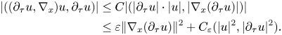
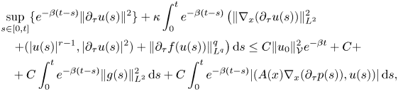
The central role in our study plays assumption (1.5) and the related second energy identity:

Here and below $(u,\,v)$ stands for the standard inner product in $L^2(\Omega )$
 . The only nontrivial term in (1.9), which prevents us to complete the estimate, is the one containing the inertial term. In order to handle it, we derive the Strichartz type estimate for the $L^2_{loc}(\mathbb {R}_+,\,L^\infty (\Omega ))$
 -norm of the solution $u$
 . Obtaining this estimate is the most difficult and most technical part of the paper. We get this result applying the nonlinear localization technique directly to the non-stationary equation (1.1) with the inertial term. In contrast to the previous results related with the stationary equation (1.6), we are unable to get the maximal regularity estimate for (1.1) (i.e. to verify that every term in the equation belongs to the space $L^2_{loc}(\mathbb {R}_+,\,L^2(\Omega ))$
 ), but the obtained Strichartz type estimate mentioned above is enough for our purposes. This allows us to establish the following key result.
Theorem 1.1 Let the assumptions (1.3), (1.5), and (1.2) hold with $r>3$ and let $u_0\in \Phi$
 , where

Then the unique weak solution $u(t)$ of problem (1.1) satisfies the following estimate:
for some positive constant $\beta$ and a monotone function $Q$
 which are independent of $u_0$
 and $t$
 .
.
In particular, if the right-hand side $g(t)$ is bounded as $t\to \infty$
 in the sense that

estimate (1.11) gives us a uniform dissipative estimate

for some new monotone function $Q$ and this, in turn, allows us to study the long-time behaviour of solutions of (1.1) in terms of uniform attractors for the cocycle generated by equation (1.1), see [Reference Babin and Vishik3, Reference Carvalho, Langa and Robinson7, Reference Chepyzhov and Vishik8, Reference Kloeden and Rasmussen18, Reference Zelik42] and references therein.
Note that, in contrast to the standard situation, it looks difficult here to establish the existence of a compact uniformly absorbing set for the corresponding cocycle based only on the compactness of Sobolev embeddings, so we utilize the energy method (see [Reference Ball4]), the central part of which is to establish the energy identity (1.9) for any weak solution of (1.1). Surprisingly, this is also not straightforward since the regularity of a weak solution provided by theorem 1.1 is not enough to justify the multiplication of (1.1) by $\partial _t u$ . We overcome this difficulty using the convexity argument and the fact that the energy in (1.9) is a compact perturbation of a uniformly convex functional. As a result, we prove that, under the mild extra assumption that the external forces $g$
 are weakly normal, see [Reference Lu21–Reference Ma, Zhong and Song24, Reference Zelik41] and also definition 5.6 below, the cocycle generated by solution operators of equation (1.1) possesses a uniform attractor in the strong topology of $\Phi$
 and is generated by all complete bounded solutions, see §5 below.
The paper is organized as follows. In §2 we consider the stationary case of equation (1.1) and refine the results of [Reference Kalantarov and Zelik16] based on the non-linear localization technique. The obtained results are crucial for the study of the non-autonomous case.
In §3, which is the key section of our paper, we apply the non-linear localization technique to the non-autonomous equation (1.1) in order to get the above mentioned Strichartz type estimate and to give the proof of theorem 1.1. We also give a number of extra regularity results which will be essentially used later.
§4 is devoted to the verification of the energy identity (1.9). In order to do this, we utilize the convexity arguments and extend the ideas of [Reference Mielke and Zelik29] to our case.
Finally, in §5, we briefly recall the main ideas and concepts of the attractors theory for non-autonomous dynamical systems and verify the existence of a uniform attractor for the cocycle related with equation (1.1) in the phase space $\Phi$ .
.
2. The stationary case
In this section, we consider the following stationary version of the Brinkman-Forchheimer equation:

Here $u=(u_1(x),\,u_2(x),\,u_3(x))$ and $p=p(x)$
 are an unknown velocity vector field and pressure respectively, $\Omega \subset \mathbb {R}^3$
 is a bounded domain with a sufficiently smooth boundary, $f\in C^1(\mathbb {R}^3,\,\mathbb {R}^3)$
 is a given nonlinearity which satisfies the following dissipativity and growth restrictions:

for some given positive constants $\kappa$ and $C$
 and the exponent $r\in [1,\,\infty )$
 , and $g\in L^2(\Omega )$
 is a given external force. We also assume that the mean of pressure is equal to zero
We are mainly interested in the case $r\gg 1$ , where the nonlinearity is not subordinated to the linear part of the equation. Note that this problem under the similar assumptions has been already considered in [Reference Kalantarov and Zelik16], however, the estimates obtained there are not enough for our purposes, so in the present section, we refine them as well as deduce a number of new ones.
We start with the standard energy estimate.
Proposition 2.1 Let the nonlinearity $f$ satisfy (2.2) and $g\in L^2(\Omega )$
 . Let also $u$
 be a sufficiently smooth solution of equation (2.1). Then, the following estimate holds:

where $1/{(r+1)}+ac1/q=1$ and $C$
 is a positive constant which is independent on $u$
 .
.
Proof. Multiplying equation (2.1) by $u$ , integrating over $\Omega$
 and using the Hölder inequality, we get the energy identity

where $(U,\,V)$ stands for the standard inner product in $[L^2(\Omega )]^3$
 . Using our assumptions on $f$
 , we deduce from here that

for some positive constant $C$ . To complete the proof of the proposition, we write out equation (2.1) as a linear equation

and apply the maximal $L^q$ -regularity result for solutions of the linear Stokes equation, see e.g. [Reference Galdi11]. Together with the already obtained estimate for the $L^q$
 -norm of $f(u)$
 , this give us the desired control of the $W^{2,q}$
 -norm of $u$
 as well as the $L^q$
 -norm of pressure $p$
 .
.
At the next step, we want to obtain higher energy estimates for the solutions of (2.1). In the case of periodic boundary conditions, we get such estimates by multiplying the equation by $\Delta _x u$ . However, this does not work at least in the straightforward way for the Dirichlet BC since the term $(\nabla _x p,\,\Delta _x u)$
 becomes out of control because of non-trivial boundary terms, which appear under the integration by parts. Following [Reference Kalantarov and Zelik16], we use the nonlinear localization technique in order to overcome the problem.
Theorem 2.2 Let $u$ be a sufficiently smooth solution of equation (2.1). Then, the following partial regularity estimate holds:
where the constant $C$ is independent of $u$
 and $g$
 . Moreover, the following conditional result holds:

Proof. We divide the proof of this theorem on several steps.
Step 1. Interior regularity. Let $\varphi (x)$ be a sufficiently smooth cut-off function which vanishes near the boundary and equal to one identically outside of the $\varepsilon$
 -neighbourhood of $\partial \Omega$
 and which satisfies the inequality

Since the domain $\Omega$ is smooth, such a function exists for every $\varepsilon >0$
 .
.
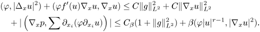
Let us multiply equation (2.1) by $\sum \partial _{x_i}(\varphi \partial _{x_i}u)$ and transform the most complicated term containing pressure as follows:

The last term in the RHS is easy to estimate using (2.3):

To estimate the first term, we take the divergence from both sides of equation (2.1) and obtain the Poisson equation for pressure:
Thus, integrating by parts again and using the growth restrictions on $f$ and estimate (2.4), we arrive at
Using that $|\nabla _x \varphi |\le C\varphi ^{1/2}$ , we transform the last term as follows:
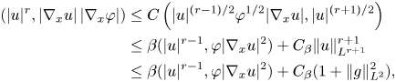
where $\beta >0$ is arbitrary. Combining the obtained estimates, we get

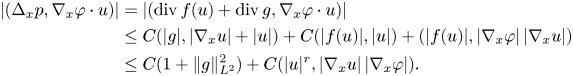
It is now not difficult to complete the interior estimate. Indeed, multiplying equation (2.1) by $\sum _i\partial _{x_i}(\varphi \partial _{x_i}u)$ and arguing in a standard way, with the help of (2.12), we get
Finally, due to our assumptions, $f'(u)\ge \kappa (|u|^{r-1}+1)$ , so fixing $\beta <\kappa /2$
 , we arrive at the desired estimate

which gives the interior $H^2$ -regularity.
Step 2. Boundary regularity: tangential directions. We now look at a small neighbourhood of the boundary $\partial \Omega$ . We introduce a family of orthogonal vector fields $\tau ^1$
 , $\tau ^2$
 and $n$
 in $\bar \Omega$
 which are non-degenerate near the boundary and such that $\tau ^i\big |_{\partial \Omega }$
 are tangent vector fields and $n\big |_{\partial \Omega }$
 is a normal vector field. Note that $n(x)$
 is globally defined, but $\tau ^i$
 are in general only locally defined, so being pedantic we need to use the cut-off procedure in order to localize them. In order to avoid technicalities, we however will assume that they are globally defined. Let $\tau =(\tau _1,\,\tau _2,\,\tau _3)$
 be one of the vectors $\tau ^1$
 or $\tau ^2$
 . Then, we may define the corresponding differential operators
Our idea is to multiply equation (2.1) by $\partial _\tau ^*\partial _\tau u$ and get the $H^1$
 -norm of $\partial _\tau u$
 analogously to Step 1 using the fact that $\partial _\tau u\big |_{\partial \Omega }=0$
 . As before, we start with the most complicated term related with the pressure:

Here and below, we denote by $[D_1,\,D_2]$ the commutator of two differential operators $D_1$
 and $D_2$
 , i.e. $[D_1,\,D_2]u:=D_1(D_2u)-D_2(D_1)u$
 . Let us first estimate the term with the commutator using integration by parts and the fact that $u$
 is divergence free:

for some smooth (and therefore bounded) matrices $A$ and $B$
 . The remaining term is analogous, but even simpler

Thus, we have proved the following key relation:

for some smooth matrices $\widetilde A(x)$ and $\widetilde B(x)$
 . We now turn to the term containing the Laplacian:

It only remains to estimate the term containing commutator. It is a sum of second and first order differential operators, so integrating by parts again in the second order part, we arrive at

and, therefore, we end up with the estimate
The non-linear term is estimated in a standard way:

and combining the obtained estimates together, we arrive at

In order to estimate the term with pressure in the right-hand side, we differentiate equation (2.1) along $\tau$ and write the obtained expression in the following form:
From estimate (2.3), we know that

where we have used that $[\partial _\tau,\,\Delta _x]$ and $[\partial _\tau,\,\operatorname {div}]$
 are second and first order operators respectively. Also $\|H\|_{W^{1,q}}\le C\|g\|_{L^q}$
 . We now decompose

where

where $H_3=H$ and $H_1=H_2=0$
 . Then, due to the $L^q$
 and $H^{-1}$
 regularity estimates for the Stokes operator, see e.g. [Reference Galdi11], we have

Inserting these estimates to (2.19), we arrive at
It only remains to estimate the last term via the Hölder inequality:

where we have used that $1-\frac q2=1-\frac {r+1}{2r}=\frac {r-1}{2r}$ and $q(r-1)\frac {2r}{r-1}=2(r+1)$
 . Inserting the obtained estimate to the right-hand side of (2.22), we end up with the desired estimate for tangential derivatives:

Step 3. Interpolation and regularity in normal directions. Let $U:=\nabla _x u$ . Then, estimates and (2.3) and (2.25) give us

Recall that we are now doing estimates in a small neighbourhood of the boundary only (inside of the domain $\Omega$ we already have better control of the $H^2$
 -norm of $u$
 from the proved interior estimate). Thus, using the partition of unity, we may fix a small neighbourhood of containing a piece of the boundary and the straighten it by an appropriate diffeomorphism in such a way that in new coordinates $y=(y_1,\,y_2,\,y_3)$
 . The direction $y_1$
 corresponds to the normal direction $\vec n$
 and the variables $y_2$
 , and $y_3$
 correspond to the tangent directions. Then, estimate (2.26) reads

After that we may use the interpolation for anisotropic Sobolev spaces:

where
so $\theta =\frac 13$ , see e.g. [Reference Rákosnik34] or [Reference Besov, Ilin and Nikolski5]. Thus, reminding that $U=\nabla _x u$
 ,we end up with the desired partial regularity estimate

Indeed, inside of the domain $\Omega$ , we have better estimate with the exponent $6$
 instead of $3q$
 due to the proved interior regularity and estimate (2.29) in a small neighbourhood of the boundary follows from the interpolation mentioned above. Thus, estimate (2.6) is proved and we only need to check (2.7). To this end, we first note that, due to the interior estimate (2.14), our assumptions on $f$
 and the Sobolev embedding $H^1\subset L^6$
 , we have
Thus, we only need to look at a small neighbourhood near the boundary. Using the refined Sobolev estimate

which holds for every $v\in H^1_0((0,\,1)^3)$ and taking $v=|u|^{(r+1)/2}$
 , analogously to (2.30), we get
Combining this estimate with (2.25), we end up with the desired estimate (2.7) and finish the proof of the theorem.
We are now ready to complete the maximal $L^2$ -regularity estimate for the solutions of equation (2.1).
Corollary 2.3 Let $u$ be a sufficiently smooth solution of equation (2.1). Then the following estimate holds:

where the constant $C$ is independent of $u$
 and $g$
 and $s=\max \{2,\,\frac {4(2-q)}{3q-2}\}$
 .
.
Proof. Using estimates (2.3), (2.7) and the interpolation inequality, we infer that
Since $1< q<2$ , using the Young inequality, we may rewrite the last inequality in the form
where $\nu >0$ is arbitrary. Treating now the term $f(u)$
 in (2.1) as external forces and applying the maximal $L^2$
 -regularity estimate to the linear Stokes equation, we arrive at
Moreover, from the equation (2.1) we have
Finally, in order to estimate the last term in the right-hand side, we multiply equation (2.1) by $\Delta _x u$ and integrate over $x\in \Omega$
 . This gives
Fixing $\nu >0$ small enough, we deduce that

which together with (2.35) and (2.36) finish the proof of the corollary.
We now briefly discuss the existence and uniqueness of a solution for (2.1). We start with weak solutions. To this end, we introduce the standard notation for the Navier–Stokes equations theory, namely, space $\mathcal {D}_\sigma (\Omega )$ of divergence free $C^\infty$
 -smooth vector fields in $\Omega$
 vanishing near the boundary as well as the spaces $\mathcal {H}$
 and $\mathcal {V}$
 which are the closure of $\mathcal {D}_\sigma (\Omega )$
 in $[L^2(\Omega )]^3$
 and $[H^1(\Omega )]^3$
 respectively. The space $\mathcal {V}^{-1}$
 is defined as a dual space to $\mathcal {V}$
 with respect to the duality generated by the standard inner product in $\mathcal {H}$
 . Then, for every external force $g\in \mathcal {V}^{-1}+L^q(\Omega )$
 , we say that $u$
 is a weak solution of (2.1) if $u\in \mathcal {V}\cap L^{r+1}(\Omega )$
 and satisfies equation (2.1) in the sense of distributions, i.e.

for all test functions $\varphi \in \mathcal {D}_\sigma (\Omega )$ . As usual, see e.g. [Reference Galdi11], the pressure $p$
 can be restored using $L^q$
 and $H^{-1}$
 regularity estimates for the linear Stokes operator, so we may also claim that $p\in L^2(\Omega )+W^{1,q}(\Omega )$
 for any weak solution $u$
 .
.
The existence of a weak solution is straightforward and can be done using, for instance, the Galerkin approximation method, see e.g. [Reference Galdi11, Reference Temam37]. The uniqueness also straightforward due to our monotonicity assumption on $f$ and the density of $\mathcal {D}_\sigma (\Omega )$
 in $\mathcal {V}\cap L^{r+1}$
 proved in [Reference Galdi11] (see also [Reference Gallbally and Zelik10] for an alternative proof). So, we discuss only the further smoothness of weak solutions.
Corollary 2.4 Let $g\in L^2(\Omega )$ . Then, the unique weak solution $u$
 of problem (2.1) belongs to $H^2(\Omega )$
 , the corresponding pressure $p\in H^1(\Omega )$
 and all of the estimates stated above hold.
Proof. We first note that, due to the uniqueness of weak solutions, it is enough to construct a regular solution $u\in H^2(\Omega )$ for any $g\in L^2(\Omega )$
 and this will automatically exclude the existence of weak non-smooth solutions. Since the nonlinear localization seems to not work on the level of Galerkin approximations (at least we do not know how to obtain uniform estimates for higher norms), we need to use the alternative methods. For instance, we may use the continuation by the parameter methods based on the Leray–Schauder degree theory. Indeed, let us consider the family of equations of the form (2.1) depending on a parameter $\varepsilon \in [0,\,1]$
 :
:

Using the Leray–Helmholtz projector $\Pi$ and the invertibility of the Stokes operator $A:=\Pi \Delta$
 , we may rewrite equation (2.39) in the equivalent form
Let us assume that $g\in H^1$ and consider equation (2.40) as an equality in $H^3(\Omega )$
 . Then, due to the embedding $H^3(\Omega )\subset C^1(\Omega )$
 and the $H^1\to H^3$
 regularity of the solutions of the linear Stokes operator, see [Reference Galdi11], the right-hand side of (2.40) is a compact and continuous operator in $H^3(\Omega )$
 , so the Leray–Schauder degree theory works and we only need to obtain the uniform with respect to $\varepsilon \in [0,\,1]$
 estimates for the $H^3$
 -solutions of (2.40) or, which is the same, $H^3$
 -solutions of (2.39).
To get this estimate, we note that now we a priori know that the solution $u=u_\varepsilon$ is in $H^3$
 and the corresponding pressure $p_\varepsilon \in H^2$
 (by the regularity of the Leray–Helmholtz projector). Since all the above estimates related with nonlinear localizations obviously hold for such solutions, we may apply corollary 2.3 to equation (2.39), which gives us the estimate of the $H^2$
 -norm of $u$
 . Moreover, it is not difficult to see that this estimate is unform with respect to $\varepsilon$
 , so we end up with

where the function $Q$ is independent of $\varepsilon$
 . After that, using the embedding $H^2(\Omega )\subset C(\Omega )$
 , we get the control of the $H^1$
 -norm of $f(u)$
 and, due to the regularity of the Stokes operator, we finally get the desired uniform a priori estimate in the $H^3$
 -norm. Thus, we have proved the existence of $H^3$
 -solution of problem (2.1) under the extra condition that $g\in H^1$
 . Since the $H^2$
 -norm estimate of $u$
 depends only on the $L^2$
 -norm of $u$
 , we may approximate a given external force $g\in L^2$
 by a sequence $g_n\in H^1$
 , construct the associated solution $u_n$
 and pass to the limit $n\to \infty$
 . This will give us the desired $H^2$
 -solution and finish the proof of the corollary.
Let us now consider the stationary Navier–Stokes–Brinkman–Forchheimer equation:

Then, the weak solution of this problem is defined exactly as in the case of equation (2.1). Moreover, we have the energy estimate (2.4) for such solutions due to the cancellation $((u,\,\nabla _x) u,\,u)=0$ . The existence of a weak solution can be obtained after that, e.g. by the Galerkin method. The next corollary tells us when every such solution is automatically smooth.
Corollary 2.5 Let $g\in L^2(\Omega )$ . Then any weak solution $u$
 of problem (2.41) belongs to $H^2(\Omega )$
 and the pair $(u,\,p)$
 possesses the following estimate:

where the function $Q$ is independent of $u$
 and $g$
 .
.
Proof. We first derive estimate (2.42) assuming that $u$ is smooth enough, e.g. $u\in H^2$
 . To this end, we interpret equation (2.41) and (2.1) with the right-hand side $\widetilde g:=g+(u,\,\nabla _x)u$
 and apply estimate (2.32) to it. In addition, analyzing the proof of this estimate, we see that the term containing $\|\widetilde g\|_{L^q}$
 in the right-hand side of it comes from the corresponding estimate of $\|f(u)\|_{L^q}$
 and this control we already proved for (2.41), so we may replace $\widetilde g$
 by $g$
 in this part of the estimate and arrive at

Using the appropriate interpolation inequality together with (2.4), we estimate

and, therefore,

Since $s=\max \{2,\,\frac {4(2-q)}{3q-2}\}<4$ for $1\le q\le 2$
 , the last estimate implies (2.42). Thus, the $H^2$
 a priori bound for a sufficiently smooth solution of (2.41) is obtained. The existence of such a solution can be verified, e. g. using again the Leray–Schauder degree theory, see the proof of corollary 2.4, and we only need to check that any weak solution is actually smooth.
In contrast to corollary 2.4, we do not expect the uniqueness of a weak solution for problem (2.41) due to the presence of the non-monotone inertial term. In order to overcome this problem, we add an artificial term $Lu$ with big $L$
 in both sides of equation (2.41) and consider the auxiliary problem

where $u$ is a fixed weak solution of (2.41). Then, since $\bar g\in L^2$
 and the new nonlinearity $f(v)+Lv$
 satisfies all of the assumptions posed on $f$
 , this problem possesses a smooth solution $v\in H^2$
 . On the other hand, $u$
 is still a weak solution of this problem and we only need to check that $u=v$
 . This will be true if $L$
 is large enough to compensate the non-monotonicity of the inertial term. Indeed, let $w=u-v$
 . Then, this function solves

Multiplying this equation by $w$ , integrating by $x\in \Omega$
 and using the monotonicity of $f$
 together with the cancellation $((u,\,\nabla _x)w,\,w)=0$
 , we arrive at

and we see that the uniqueness holds if $L>C_2\|v\|^4_{H^1}$ . This finishes the proof of the corollary.
3. The non-stationary case
In this section, we turn to study the non-stationary Brinkmann–Forchheimer–Navier–Stokes equation of the form:

where $u_0\in \mathcal {V}$ and
and
Our general plan to tackle this problem is similar to what we did in § 2. Namely, we first obtain the basic energy estimate (by multiplying the equation by $u$ ) and after that improve the regularity of a solution using the nonlinear localization technique. In the case where $g$
 is regular enough in time, e.g. $g\in C^1_b(\mathbb {R},\,L^2(\Omega ))$
 , one can get the control of the $C_b(\mathbb {R}_+,\,L^2(\Omega ))$
 -norm of $\partial _t u$
 by differentiating the equation in time and multiplying it by $\partial _t u$
 , see [Reference Kalantarov and Zelik16] for the details. This will reduce the problem to the autonomous one which is considered in the previous section.
However, the regularity of (3.2) is not sufficient to proceed in such a way and we need to apply the nonlinear localization technique to the non-stationary equation (3.1) in direct way. As we will see below, the interior estimates as well as regularity in tangential directions can be extended to the non-stationary case with some extra technicalities related with the inertial term. In contrast to this, the obtained regularity in time is insufficient to derive reasonable analogue of estimate (2.32) and get the regularity in normal direction. For this reason, we failed to get full $H^2$ -maximal regularity in the non-stationary case and do not know whether or not it holds (even in a ‘simple’ case of periodic boundary conditions), but the obtained results are enough to establish the well posedness of (3.1) in the phase space $\Phi$
 under the extra assumption that the nonlinearity $f$
 is gradient, i.e.
for some $F\in C^2(\mathbb {R}^3)$ . Again, we do not know whether or not the problem (3.1) is globally well-posed without this assumption although some of our estimates remain true without it. We also relax slightly assumption (2.2) in order to include non-monotone nonlinearities. Namely, we assume from now on that

for some positive constants $\kappa$ , $C$
, $C$ and $L$
 .
.
We start with the non-stationary analogues of basic energy estimates.
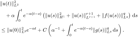
Proposition 3.1 Let the assumptions (3.4) and (3.2) hold and let $u$ be a sufficiently smooth solution of (3.1). Then, the following estimate holds:
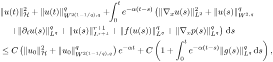
where the positive constants $C=C_\alpha$ and $0<\alpha <\alpha _0$
 can be chosen arbitrarily (where $\alpha _0$
 is small enough). All constants are independent of $t$
 and $u$
 .
.
Proof. We multiply equation (3.1) by $u$ and integrate over $x\in \Omega$
 to get

Then, using assumption (3.4) together with the Hölder and Poincare inequalities, we arrive at

where $C$ and $\alpha$
 are positive constants which are independent of $t$
 and $u$
 . Integrating this inequality, we have
Thus, the basic energy estimate is proved (note that the assumption $r\ge 3$ is nowhere used here). To complete estimate (3.5), we need to rewrite equation (3.1) in the form of a linear non-stationary Stokes equation:

and to apply the standard $L^q$ -maximal regularity estimate to this equation. This gives

where $C$ and $\alpha$
 are some constants and $|\alpha |$
 is small enough, see e.g. [Reference Solonnikov35]. So, it only remains to estimate the norm of $g_u(s)$
 in the right-hand side. Moreover, the term containing $f(u)$
 is already estimated and we only need to estimate the inertial term. To this end, we need the assumption $r\ge 3$
 which allows us to use the Hölder inequality in the form

since $\frac {2q}{2-q}=\frac {2(r+1)}{r-1}\le r+1$ if $r\ge 3$
 . Thus, the inertial term is also controlled by (3.8) and this estimate together with (3.10) give the desired estimate (3.5) and finish the proof of the proposition.
Analogously to the stationary case, we define a weak solution $u(t)$ of problem (3.1) as a function which belongs to the space

which satisfies (3.1) in the sense of distributions, i.e.

for all $\varphi \in C_0^\infty (\mathbb {R}_+\times \Omega )$ with $\operatorname {div} \varphi (t) = 0$
 . Here and below $\left \langle u,\,v\right \rangle :=\int _{\mathbb {R}}(u(t),\,v(t))\,{\rm d}t$
 and $C([0,\,\infty ),\,\mathcal {H}_w)$
 means the space of $\mathcal {H}$
 -valued functions $u(t)$
 , $t\in \mathbb {R}_+$
 , which are continuous in time in the weak topology of $\mathcal {H}$
 . We summarize the known facts about the existence and uniqueness of such solutions in the following proposition.
Proposition 3.2 Let the nonlinearity $f$ satisfy assumption (3.4) for some $r\ge 1$
 . Then, for every $u_0\in \mathcal {H}$
 and every $g\in L^q_{loc}([0,\,\infty ),\,L^q(\Omega ))$
 , problem (3.1) possesses at least one weak solution $u$
 which satisfies the energy estimate (3.8). If, in addition, $r>3$
 , then the weak solution of this problem is unique. Moreover, if $r>3$
 and $u_0\in \mathcal {H}\cap W^{2(1-1/q),q}(\Omega )$
 , then estimate (3.5) holds for the weak solution of (3.1).
Proof. Indeed, the existence of a solution follows in a standard way from estimate (3.8) using, e.g. Galerkin approximations. The uniqueness of a solution is known for $r>3$ only. First of all, we use this assumption in order to check that the inertial term is in $L^q$
 , see (3.11). After that, we justify the multiplication of equation (3.1) by $u$
 as well as the multiplication of for difference of two weak solutions $u$
 and $v$
 by $u-v$
 and this gives us the following identity for the difference $w:=u-v$
 :
:

see [Reference Gallbally and Zelik10, Reference Kalantarov and Zelik16] for the details. Then, using the integration by parts, we estimate the inertial term as follows

Moreover, using assumption (3.4) on the nonlinearity, we arrive at

for some positive constants $\kappa '$ and $C_{r,\kappa }$
 (here we have used that $r>3$
 again). Inserting these estimates into (3.12), we have
and the Gronwall inequality gives us that $w=0$ which proves the uniqueness. Finally, if $u_0\in \mathcal {H}\cap W^{2(1-1/q),q}(\Omega )$
 , we may apply the maximal $L^q$
 -regularity estimate (3.10) to the linear Stokes equation (3.9) and verify that the unique weak solution (3.9) satisfies (3.5). This finishes the proof of the proposition.
We are now ready to state and prove the main result of this section, which gives the global well-posedness of problem (3.1) in the phase space $\Phi =\mathcal {V}\cap L^{r+1}(\Omega )$ .
.
Theorem 3.3 Let $u_0\in \Phi :=\mathcal {V}\cap L^{r+1}(\Omega )$ , the nonlinearity $f$
 satisfy (3.4) and (3.3) for some $r>3$
 and let $g$
 satisfy (3.2). Then the weak solution $u(t)\in \Phi$
 for all $t\ge 0$
 and satisfies the following estimate:

where $\|u\|_\Phi ^2:=\|u\|_{\mathcal {V}}^2+\|u\|_{L^{r+1}}^{r+1}$ , $Q$
, $Q$ is a monotone function and $\beta$
 is a positive constant, both are independent of $t$
 and $g$
 and we put $0$
 instead of $t-1$
 if $t\le 1$
 . Moreover, if we only assume that $u_0\in \mathcal {H}$
 , then $u(t)\in \Phi$
 for all $t>0$
 and the following estimate holds for $t\ge 1$
 :
:

Proof. Of course, the analogue of the smoothing property (3.14) holds for all $t>0$ with the function $Q$
 depending also on $1/t$
 and we state the smoothing property for $t\ge 1$
 just in order to avoid extra technicalities.
We first assume that $u$ is a sufficiently smooth solution of (3.1), for instance,

and derive the desired estimates for it. We divide the proof on several steps.
Step 1. Interior estimates. This step is almost identical to Step1 in the proof of theorem 2.2. Indeed, let $\varphi$ be the same as in that step. Multiplying equation (3.1) by $-\sum _{i}\partial _{x_i}(\varphi \partial _{x_i}u)$
 , we arrive at

Thus, we just have an extra term in the right-hand side of (3.16) which is related with the inertial term which should be properly estimated and also we now have

with the extra term related with the divergence of the inertial term (in comparison with (2.9)). Both of the extra terms are not difficult to control. Indeed,

The extra term in the expression for the Laplacian of pressure $p$ , after inserting it into the right-hand side of (3.16) gives us the term

which can be estimated exactly as in (3.17). Combining all of the estimates together, we arrive at
Finally, integrating this relation in time and using (3.5), we arrive at the desired interior estimate
for some positive constants $C$ and $\alpha$
 .
.
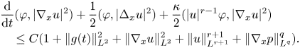
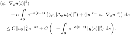
Step 2. Boundary regularity: tangential directions. Analogously to § 2, we multiply equation (3.1) by $\partial ^*_\tau \partial _\tau u$ and integrate over $x\in \Omega$
 . Then, in comparison with (2.19), we will have an extra good term $1/2 {{\rm d}}/{{\rm d}t}\|\partial _\tau u\|^2_{L^2}$
 as well as the term $((u,\,\nabla _x)u,\,\partial _\tau ^*\partial _\tau u)$
 related with the extra inertial term, which can be estimated as follows:

Furthermore, integrating by parts, we get
Thus, using again that $r>3$ , we arrive at

where $\varepsilon >0$ is arbitrary, and, therefore, this extra term is under the control and, arguing as in the stationary case, we arrive at

Integrating this inequality in time and using (3.8), after the standard transformations, we arrive at
where $\kappa$ , $\beta$
 and $C$
 are some positive constants, which are independent of $t$
 and $u$
 . Thus, we only need to estimate the term, containing pressure. To this end, we introduce a function $G=G(t)$
 as a solution of the linear Stokes equation:

Then, using the $L^2$ -maximal regularity estimate for the linear Stokes equation, see [Reference Solonnikov35], we end up with

for some positive constants $\beta _1>\beta$ , and $C$
 (and we also have the $L^q$
 -version of this estimate). We also introduce a new function $v:=u-G$
 which also solves the linear Stokes equation:

Differentiating this equation with respect to $\tau$ and denoting $w:=\partial _\tau v$
 and $p_w:=\partial _\tau p_v$
 , we arrive at
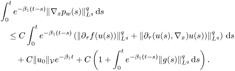
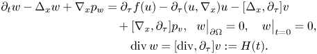
Our plan is to apply the $L^q$ -maximal regularity estimate to this linear non-homogeneous Stokes equation. Indeed, from estimates (3.5) and (3.24), we only know that

and the $L^q$ -norm in time from the left-hand side is under the control. However, this is not enough in general to get the maximal $L^q$
 -regularity estimate (in general, we need $\partial _t H$
 to belong to $L^q(0,\,t;L^q)$
 , see e. g. [Reference Filinov and Shilkin9] for the counterexample). Fortunately, the function $H(t)$
 in (3.26) has a special structure which allows us to overcome this problem. Namely, it is not difficult to see that

Important is that $W\big |_{\partial \Omega }=0$ . Therefore, we may subtract the function $W$
 from the solution $w$
 and get a new linear Stokes problem for the function $\bar w:=w-W$
 :
:
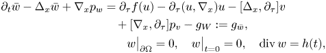
where $g_W:=\partial _t W-\Delta _x W$ . Since both $W$
 and $h$
 are proportional to $v$
 , we have the control of the $L^q$
 -norms of $G_W$
 and $\partial _t h$
 from (3.5). Moreover, since

and $p=p_G+p_v$ , all terms with commutators are also controlled by (3.5). We actually need not to estimate $\partial _\tau f(u)$
 since this term is presented in the left-hand side of (3.23) and will be finally cancelled out. However, we still need to estimate the most complicated term related with the inertial term in (3.28), but we prefer to postpone this estimate and first complete the exclusion of pressure. To this end, we apply the $L^q$
 -regularity estimate to problem (3.28), see [Reference Filinov and Shilkin9] and get

Using the obvious estimate

where $\alpha >\beta _1>0$ and the constant $C^*$
 depends only on $\alpha$
 and $\beta$
 , together with estimate (3.5) and the $L^q$
 -version of estimate (3.24), we arrive at
We are now ready to return to estimation of the last term in (3.23). Namely,

where $\nu >0$ is arbitrary. Using the obtained estimates (3.31) and (3.24) together with (3.30), we exclude the pressure from (3.23) and get
Moreover, the last term in this estimate can be further simplified. Namely,

and

Since $\frac {2q}{q-2}=\frac {2(r+1)}{r-1}< r+1$ if $r>3$
 , this term is under the control. The third term in the right-hand side of (3.34) can be estimated analogously using the fact that the commutator $[\nabla _x,\,\partial _\tau ]$
 is a first order differential operator. So, we only need to estimate the first term. We will do this with the help of (2.29), the Hölder inequality and the fact that $\frac {3q}2\le 2$
 , namely,
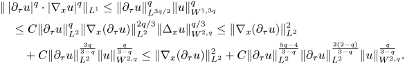
Crucial for us is the fact that $\frac {5q-4}{3-q}<2$ for $q<\frac {10}7$
 and therefore, due to our assumptions, $q<\frac 43<\frac {10}7$
 , so the number $m:=2- \frac {5q-4}{3-q}$
 is always positive. In addition, the first term in the right-hand side of (3.35) is not dangerous since it is absorbed by the corresponding term in the left hand side of (3.33), so we only need to estimate the integral

To this end, we use that the exponents $\frac {2(2-q)}{3-q}$ and $\frac q{3-q}$
 are such that, due to the Young inequality

and, therefore,

Inserting this estimate to the right-hand side of (3.33) and using estimate (3.5) with $\alpha =\beta /2$ , we finally end up with the following estimate:
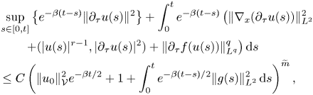
where $\widetilde m:=\max \{1,\,2/m\}$ . This finishes the boundary regularity estimate in tangential directions.
Step 3. Key interpolation estimate. Namely, we start with the Gagliardo–Nirenberg inequality:
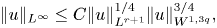
since $\frac 34-3\left (\frac 1{4(r+1)}+\frac 1{4q}\right )=0$ , see e.g. [Reference Machihara and Ozawa25] or [Reference Adams and Fournier2]. This inequality, together with (2.29), give us
where we have used that $1=\frac 1{2(r+1)}+\frac 1{2q}+\frac 12$ . Using estimates (3.5) and (3.37), we get the desired estimate

Step 4. $\Phi$ -energy estimate. Till that moment, we have nowhere used our extra assumption that the nonlinearity $f$
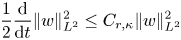
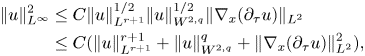
 is gradient, but it is essentially used at this step. Indeed, we now multiply equation (3.1) by $\partial _t u$
 and integrate over $x\in \Omega$
 . This gives
where $L$ is such that $F(u)+L|u|^2\ge 0$
 (it exists due to assumption (3.4)). Note that assumption (3.4) implies also that

for some positive constants $\kappa _i$ and $C_i$
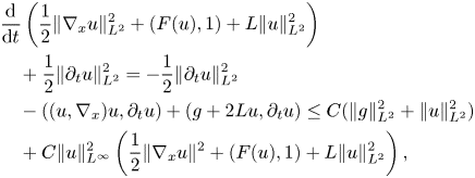
 . Therefore, estimate (3.39) allows us to apply the Gronwall inequality to (3.40) and to get the following control:
We will use this estimate for $0\le t\le 1$ only since it is growing in time even if $g(t)$
 is bounded and, therefore, is not convenient for study the attractors. Combining (3.42) with (3.39) and (3.5), we arrive at the following estimate for $t\in [0,\,1]$
 :
:

for some monotone increasing function $Q$ . For $t\ge 1$
 , we will use the following smoothing estimate:

for some new monotone function $Q$ . This estimate is a standard corollary of (3.43) and (3.5). Indeed, from (3.5), we know that

Therefore, there exists $t_0\in [0,\,1]$ (depending on $u$
 ) such that

Applying after that estimate (3.43) on the time interval $t\in [t_0,\,1]$ , we arrive at (3.44). In turn, combining estimates (3.43) (on interval $t\in [0,\,1]$
 ) with estimate (3.44) (which will give us the estimate of the $H^1\cap L^{r+1}$
 -norm of $u(t)$
 through the $L^2$
 -norm of $u(t-1)$
 , $t\ge 1$
 ) together with the dissipative estimate (3.5), we end up with the desired estimates (3.13) and (3.14). The estimate for the $L^2$
 -norm of $\partial _t u$
 in them follows immediately by integrating (3.40) in time.
Step 5. $\Phi$ -regularity of solutions. We recall that all previous estimates were derived assuming that $u(t)$
 is a sufficiently smooth solution of (3.5), for instance, satisfying (3.15), will be enough to justify all of them (here we used that $H^2\subset C$
 in 3D, so all terms related with the nonlinearity are under the control). To get such a regular solution, we approximate the external force $g$
 and the initial data $u_0$
 by the sequences $g_n$
 and $u_0^n$
 of smooth functions. Then, as proved in [Reference Kalantarov and Zelik16], there exist an $L^\infty _{loc}(\mathbb {R}_+,\,H^2)$
 smooth solution $u_n(t)$
 of problem (3.5) where the initial data $u_0$
 and the external force $g$
 are replaced by $u_0^n$
 and $g_n$
 respectively. Moreover, since $f\in C^1$
 , it is easy to see that $\partial _t f(u_n)\in L^2_{loc}(\mathbb {R}_+,\,L^2)$
 and, therefore, the standard regularity result for the linear Stokes equation gives us that (3.15) are satisfied. For this reason, the solutions $u_n$
 satisfy estimates (3.13) and (3.14) uniformly with respect to $n$
 . Passing to the limit $n\to \infty$
 , we see that the limit unique solution $u(t)$
 of problem (3.1) also satisfies these estimates. Thus, theorem 3.3 is proved.
The next corollary is gives us slightly stronger version of estimate (3.39). This improved estimate will be used later for the attractors theory.
Corollary 3.4 Let the assumptions of theorem 3.3 hold. Then the solution $u$ of problem (3.1) satisfies the following estimate:
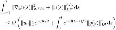
for some monotone function $Q$ and positive constant $\beta$
 .
.
Proof. We rewrite equation (3.1) in the form of a stationary problem (2.1) at every fixed time $t$ , namely,

Moreover, due to the proved theorem, the $L^2_{loc}(\mathbb {R}_+,\,L^2)$ -norm of $\widetilde g$
 is under the control. For this reason, we may apply estimates (2.3) and (2.6) to this equation (recall that the modified non-linearity $\widetilde f(u):=f(u)+Lu$
 satisfies (2.2). Then, integrating estimates (2.3) (in a power $2/q$
 ) and (2.6), we arrive at

Thus, we have got the part of the desired estimate related with the $W^{1,3q}$ -norm of $u$
 . In order to get the remaining part, we improve estimate (3.38) using that we now have estimate for the $L^2$
 -norm in time for $\|u(t)\|_{W^{2,q}}$
 and also the $L^\infty$
 norm in time for $\|u(t)\|_{L^{r+1}}$
 :
:

This estimate, together with (3.13) and (3.47) completes the desired estimate (3.45) and finishes the proof of the corollary.
Remark 3.5 In the case of periodic boundary conditions, we are able to multiply equation (3.1) by $\Delta _x u$ and the pressure term will still disappear. This immediately gives us the result of theorem 2.2 with linear function $Q$
 and also the control of the integral of $(f'(u)\nabla _x u,\,\nabla _x u)$
 . Then, from (2.7), we get the control of the $L^q$
 -norm in time of $\|f(u)\|_{L^{3q}}$
 . Combining this with the interpolation inequality (2.33) and the $L^\infty$
 -control for $\|f(u(t))\|_{L^q}$
 , we arrive at the control of the $L^{\frac {4q}{3(2-q)}}_{loc}(\mathbb {R}_+,\,L^2)$
 -norm of $f(u)$
 . In particular, if $r\le 5$
 . then $\frac {4q}{3(2-q)}\ge 2$
 and we get the $L^2$
 space-time regularity of $f(u)$
 which together with the $L^2$
 -regularity estimate for the linear Stokes problem gives us the maximal $L^2$
 -regularity for equation (3.1), namely,

Unfortunately, we do not know how to get such a regularity for $r>5$ (even in the case of periodic boundary conditions). Instead, applying the anisotropic $L^{\frac {4q}{3(2-q)}}(L^2)$
 -regularity estimate for the linear Stokes equation, we have a weakened version of the regularity (3.49) for $r>5$
 :
:

We now return to the case of Dirichlet boundary conditions. In this case, we do not have the control over the term $(f'(u)\partial _n u,\,\partial _n u)$ , so the regularity (3.50) should be further weakened. In this case, we need to use estimate (2.32) instead. Note that for $r\le 5$
 , we have the exponent $s=2$
 there and, therefore, using again that the term with the $L^q$
 -norm of $g$
 comes from the estimate of $\|f(u(t))\|_{L^q}$
 and we have the $L^\infty$
 -norm control for this term, we see that, for $r\le 5$
 , we have the maximal regularity (3.49) for the case of Dirichlet boundary conditions as well. In the case $r>5$
 , we have $s=\frac {4(2-q)}{3q-2}$
 and, therefore, the obtained regularity reads

Since $\frac {4q}{3(2-q)}>\frac {3q-2}{2-q}$ for $r>5$
 , the regularity (3.51) available for Dirichlet boundary conditions and $r>5$
 is indeed weaker than in the case of periodic boundary conditions. We do not know whether this is a drawback of the method or a real loss of regularity for the case of Dirichlet boundary conditions.
We also note that the most difficult part in the proof of the key theorem 3.3 was to estimate the $L^q$ -norm of $\partial _\tau ((u,\,\nabla _x)u)$
 . There is an alternative way to treat this term, namely, we may rewrite the inertial term in the form of $\operatorname {div}(u\otimes u)$
 and then, up to lower order terms, we will need to estimate $\operatorname {div}(u\otimes \partial _\tau u+\partial _\tau u\otimes u)$
 . Since we have the term $(|u|^{r-1} \partial _\tau u,\,\partial _\tau u)$
 in the right-hand side of (3.22), the $L^2_{loc}(\mathbb {R}_+,\,H^{-1})$
 -norm of $\partial _\tau ((u,\,\nabla _x)u)$
 is under the control. In order to complete the estimate in this way, we need the maximal regularity for the non-stationary Stokes equation in $H^{-1}$
 . Unfortunately, in contrast to the stationary case, this maximal regularity fails in general and we need some extra assumptions on the right-hand side in order to restore it. It would be interesting to check whether or not the inertial term satisfies these extra assumptions.
We finally note that the function $Q$ in the key estimate (3.13) has an exponential growth rate ($Q(z)\sim e^{Cz^{\widetilde m}}$
 ), which somehow indicates that the nonlinearities in the problem (3.1) are critical for all $r>3$
 . Since there is no such a criticality for the case of periodic boundary conditions, we expect that this also may be the drawback of the method.
4. The higher energy identity
The aim of this section is to verify the $H^1$ -energy equality, which can be formally obtained by multiplying equation (3.1) by $\partial _t u$
 and which is the key technical tool for verifying the asymptotic compactness of the dynamical processes associated with this equation. The problem here is that the proved regularity of a solution does not allow to interpret the terms $(\Delta _x u,\,\partial _t u)$
 and $(f(u),\,\partial _t u)$
 in the sense of distributions, only the inner product with their difference $(\Delta _x u-f(u)-\nabla _x p,\,\partial _t u)$
 is well-defined. Therefore, we need some accuracy with verifying the identity

Following [Reference Mielke and Zelik29], we use the convexity arguments to verify (4.1).
Theorem 4.1 Let the assumptions of theorem 3.3 hold and let $u(t)$ be the solution of (3.1). Then the function $t\to E(u(t))$
 is absolutely continuous and the identity (3.5) holds for almost all $t\in \mathbb {R}_+$
 as well as in the sense of distributions.
Proof. Note first of all that, without loss of generality, we may assume that $f'(u)\ge 0$ , so $F(u)$
 is convex. We use the following identities, which can be verified by straightforward computations:
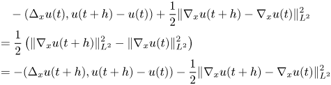
and

Note that all terms in (4.2) and (4.3) make sense as functions from $L^1_{loc}(\mathbb {R}_+)$ and these identities and the regularity of a solution $u(t)$
 is enough to justify them. Taking a sum of these two identities and using that $f'(u)\ge 0$
 , we end up with the following two-sided inequality:

Inserting the expression for $-\Delta _x u+f(u)$ from (3.1) to (4.4) and integrating over $t\in [S,\,T]$
 , we arrive at

We know that $H_u\in L^2_{loc}(\mathbb {R}_+,\,L^2)$ , $E(u)\in L^1_{loc}(\mathbb {R}_+)$
 and $u\in W^{1,2}(\mathbb {R}_+,\,L^2)$
 , therefore, we may pass to the limit $h\to 0$
 in (4.5) and get that, for almost all $S,\,T\in \mathbb {R}_+$
 , $S\le T$
 , we have the integral identity

To finish the proof of the theorem, we need to remove the condition that (4.6) holds for almost all $S\le T$ only. To this end, let us assume that the energy inequality

is already verified for all $0\le S< T$ . We recall that $u(t)$
 is weakly continuous as a function of time with values in $\Phi$
 , therefore the values of $E(u(t))$
 are well-defined for all $t\in \mathbb {R}_+$
 . Moreover, since the function $u\to E(u)$
 is convex, we have
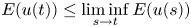
for all $t\in \mathbb {R}_+$ . In particular, this property, together with (4.7) imply that the function $t\to E(u(t))$
 is continuous from the right for all $t\in \mathbb {R}_+$
 . In turn, this ensures us that the energy equality (4.6) holds for all $0\le S< T$
 . Indeed, since (4.6) holds almost everywhere, we may find sequences $S_n\to S$
 , $S_n\ge S$
 , and $T_n\to T$
 , $T_n\ge T$
 such that (4.6) holds for $S_n$
 and $T_n$
 for all $n$
 . Passing to the limit $n\to \infty$
 , we see that it holds for $S$
 and $T$
 as well. This finishes the proof of the theorem since the energy equality (4.6), which holds for all $S$
 and $T$
 is equivalent to the absolute continuity of the function $t\to E(u(t))$
 and equality (4.1).
Thus, we only need to verify the energy inequality (4.7). Moreover, due to the uniqueness of a solution for problem (3.1), it is sufficient to verify it for $S=0$ only (the general case will follow just by replacing the initial time $t=0$
 by $t=S$
 ). To do this, we approximate the initial data $u_0\in \Phi$
 and the external force $g\in L^2_{loc}(\mathbb {R}_+,\,L^2)$
 by smooth functions $u_0^n$
 and $g_n$
 respectively. Let $u_n(t)$
 be the corresponding solutions of (3.1). Then, analogously to the end of the proof of theorem 3.3, on the one hand, the solutions $u_n(t)\in C_{loc}(\mathbb {R}_+,\,H^2)$
 and therefore, the energy equality (4.6) holds for them for every $T\ge 0$
 , i.e.

On the other hand, the solutions $u_n$ satisfy the key estimates obtained in § 3 uniformly with respect to $n$
 . These estimates guarantee that, in particular, $u_n(t)\to u(t)$
 weakly in $\Phi$
 for all $t\ge 0$
 and, by the choice of the initial data, we have the strong convergence at $t=0$
 . Therefore, without loss of generality we have

for all $t\in \mathbb {R}$ . In order to pass to the limit in the term containing $H_{u_n}$
 , we note that we also know that $\partial _t u_n\to \partial _t u$
 weakly in $L^2_{loc}(\mathbb {R}_+,\,L^2)$
 and, therefore,

Taking into account that $g_n\to g$ strongly in $L^2_{loc}(\mathbb {R}_+,\,L^2)$
 , it only remains to verify that

Indeed, due to (3.45), the functions $u_n$ are uniformly bounded in the space $L^2_{loc}(\mathbb {R}_+,\,W^{1,3q})$
 and their time derivatives are uniformly bounded in the space $L^2_{loc}(\mathbb {R}_+,\,L^2)$
 (due to theorem 3.3). Therefore, without loss of generality, we have the strong convergence of $u_n$
 in $L^2_{loc}(\mathbb {R}_+,\,W^{1-\varepsilon,3q})$
 for all $\varepsilon >0$
 . Since $W^{1-\varepsilon,3q}\subset L^\infty$
 if $\varepsilon >0$
 is small enough, we have verified that $u_n\to u$
 strongly in $L^2_{loc}(\mathbb {R}_+,\,L^\infty )$
 . Using also that $u_n$
 is bounded in $L^{8/3}_{loc}(\mathbb {R}_+,\,L^\infty )$
 (again by (3.45)), we conclude that

for all $2< r_1<\frac 83$ . We now turn to the sequence $\nabla _x u_n$
 . According to estimate (3.5) and the compactness lemma, we conclude that $\nabla _x u_n\to \nabla _x u$
 strongly in $L^q_{loc}(\mathbb {R}_+,\,W^{1-\varepsilon,q})$
 for all $\varepsilon >0$
 . Combining this result with the uniform boundedness of $\nabla _x u_n$
 in $L^2_{loc}(\mathbb {R}_+,\,L^{3q})$
 (due to (3.45)) and using that $3q>2$
 , we end up with the strong convergence

for all $1< r_2<2$ . Moreover, combining this result with the uniform boundedness of the sequence $\nabla _x u_n$
 in $L^\infty (\mathbb {R}_+,\,L^2)$
 , we see that the convergence (4.12) holds for all $1\le r_2<\infty$
 . Fixing finally the exponents $r_1$
 and $r_2$
 in such a way that $\frac 1{r_1}+\frac 1{r_2}=2$
 and using the convergences (4.11) and (4.12), we end up with the desired convergence (4.10). This convergence allows us to pass to the limit $n\to \infty$
 in the energy equality (4.9) and get the desired inequality (4.7). Thus, the theorem is proved.
We conclude this section by verifying an interesting fact about the solution $u(t)$ of (3.1), which is also based on the convexity arguments and which is important for what follows in the next section.
Corollary 4.2 Let the assumptions of theorem 3.3 hold. Then the solution $u(t)$ of the Brinkmann–Forchheimer equation is continuous in time in the strong topology of $\Phi$
 .
.
Proof. This fact is a standard corollary of the uniform convexity of the function $u\to E(u)$ as the function from $\Phi$
 to $\mathbb {R}$
 (without loss of generality, we assume that $f'(u)\ge \kappa |u|^{r-1}$
 which gives us the desired uniform convexity) and the proved energy equality. Namely, let $t_n\to t$
 , $t_n\ge 0$
 , be an arbitrary sequence of times. Then, due to the weak continuity of $u(t)$
 and the energy equality, we have

Since $u\to E(u)$ is uniformly convex, the above convergence imply that $u(t_n)\to u(t)$
 strongly in $\Phi$
 . Although this fact seems to be well-known, see e.g. [Reference Zalinescu40, Reference Zhikov and Pastukhova43], for the convenience of the reader, we present its proof below.
For the quadratic part of the functional $E(u)$ , we will use the following obvious identity:

The analogue of this identity for the nonlinearity $F$ follows from the Taylor expansions near the point $u$
 , namely,

It is not difficult to verify that

for some positive $\alpha$ and $\alpha _1$
 . Therefore, putting $u=u(x)$
 , $v=v(x)$
 in the above Taylor's expansion of the nonlinearity $F$
 and integrating it with respect to $x$
 , we get the inequality

which holds for every $u,\,v\in L^{r+1}(\Omega )$ . Combining this inequality with the identity for the quadratic part of $E_u$
 mentioned above, we end up with the key inequality

where $\alpha _3$ is a positive constant. This inequality gives us the uniform convexity of $E(u)$
 as well as the desired continuity of $u(t)$
 . Indeed, let us take $u=u(t)$
 and $v=u(t_n)$
 in this inequality. Then, we have

It only remains to note that the convergence (4.13) implies that the right hand side of (4.15) tends to zero as $n\to \infty$ , therefore, $u(t_n)\to u(t)$
 strongly in $\Phi$
 . This finishes the proof of the corollary.
5. Attractors
In this section, we will study the long-time behaviour of solutions of problem (3.1). Since the considered equation depends explicitly on time, we will construct a uniform attractor for the cocycle associated with (3.1). First of all, in order to get the dissipativity, we assume that the right-hand side $g(t)$ is in a sense bounded as $t\to \infty$
 , namely, we assume that

Following the general theory, we introduce the hull $\mathcal {H}(g)$ via
via

where $(T(h)g):=g(t+h)$ is a group of temporal shifts and $L^{2,w}_{loc}(\mathbb {R},\,L^2(\Omega ))$
 means the space $L^2_{loc}(\mathbb {R},\,L^2(\Omega ))$
 endowed with the weak topology and $[\cdot ]_W$
 stands for the closure in the space $W$
 . Then, due to assumption (5.1) and the Banach–Alaoglu theorem, the hull $\mathcal {H}(g)$
 is compact in $L^{2,w}_{loc}(\mathbb {R},\,L^2(\Omega ))$
 and, obviously, is shift invariant

From now on we endow the hull $\mathcal {H}(g)$ with the weak topology of the space $L^{2}_{loc}(\mathbb {R},\,L^2(\Omega ))$
 , so $\mathcal {H}(g)$
 is a compact metrizable topological space. In order to construct a cocycle associated with problem (3.1), we will consider a family of similar problems with all right-hand sides $\xi (t)$
 belonging to the hull $\mathcal {H}(g)$
 of the initial right-hand side $g(t)$
 , namely,

where $u_0\in \Phi$ and $\xi \in \mathcal {H}(g)$
 . Let $\mathcal {S}_\xi (t):\Phi \to \Phi$
 be the solution operator of this problem, i.e.

where $u(t)$ is a unique solution of problem (5.4), which is well-defined due to theorem 3.3. Then, the operators $\mathcal {S}_\xi (t)$
 generate a cocycle in the phase space $\Phi$
 :
:

which is a natural generalization of a solution semigroup to the non-autonomous case (see [Reference Babin and Vishik3, Reference Carvalho, Langa and Robinson7, Reference Chepyzhov and Vishik8, Reference Kloeden and Rasmussen18, Reference Temam37, Reference Zelik42] and references therein) and which is our main object to study in this section. Recall also that the cocycle property (5.5) allows us to reduce the considered cocycle to a semigroup, acting in the extended phase space $\mathbb {F}:=\Phi \times \mathcal {H}(g)$ via
via

so we may reduce the study of the non-autonomous dynamical system generated by cocycle $\mathcal {S}_\xi (t)$ to the autonomous dynamical system acting on the extended phase space $\mathbb {F}$
 . This naturally leads to the uniform attractor. We recall below the basic concepts of the attractor theory adapted to our case.
Definition 5.1 A set $B\subset \Phi$ is bounded if $\sup _{u_0\in B}\|u_0\|_{\Phi }<\infty$
 . A set $\mathbb {B}\subset \mathbb {F}$
 is bounded if $\Pi _1\mathbb {B}$
 is bounded in $\Phi$
 . Here and below $\Pi _1:\mathbb {F}\to \Phi$
 is the projector to the first component of the Cartesian product $\Phi \times \mathcal {H}(g)$
 .
.
A set $\mathcal {B}$ is a (uniformly) absorbing set for the cocycle $\mathcal {S}_\xi (t)$
 if, for any bounded set $B\subset \Phi$
 , there is a time moment $T=T(B)$
 such that

Analogously, a set $\mathcal {B}$ is a uniformly attracting set for the cocycle $\mathcal {S}_\xi (t)$
 in $\Phi$
 endowed with a suitable topology if, for any bounded set $B\subset \Phi$
 and any neighbourhood $\mathcal {O}(\mathcal {B})$
 , there exists $T=T(B,\,\mathcal {O})$
 such that

A set $\mathcal {A}_{un}$ is a uniform attractor for the cocycle $\mathcal {S}_\xi (t)$
 if
if
(1) The set $\mathcal {A}_{un}$
 is compact in $\Phi$;
(2) The set $\mathcal {A}_{un}$
is an attracting set for the cocycle $\mathcal {S}_\xi (t)$;(3) The set $\mathcal {A}_{un}$
is a minimal (by inclusion) set which satisfies properties 1) and 2).


We will consider two choices of the topology in $\Phi$ , namely, weak and strong topologies. The corresponding attractors $\mathcal {A}_{un}^w$
 and $\mathcal {A}_{un}^s$
 will be referred as weak and strong uniform attractors respectively.
In order to describe the structure of the uniform attractor, we need one more standard definition.
Definition 5.2 A function $u:\mathbb {R}\to \Phi$ is a complete bounded trajectory of the cocycle $\mathcal {S}_\xi (t)$
 which corresponds to the symbol $\xi \in \mathcal {H}(g)$
 if $\sup _{t\in \mathbb {R}}\|u(t)\|_\Phi <\infty$
 and
and

The set of all bounded trajectories of the cocycle $\mathcal {S}_\xi (t)$ which correspond to the symbol $\xi \in \mathcal {H}(g)$
 is denoted by $\mathcal {K}_\xi$
 . It is not difficult to see that a bounded $\Phi$
 -valued function $u(t)$
 , $t\in \mathbb {R}$
 , belongs to $\mathcal {K}_\xi$
 if and only if it solves equation (5.4) for all $t\in \mathbb {R}$
 , so the set $\mathcal {K}_\xi \subset C(\mathbb {R},\,\Phi )$
 is nothing else than the set of all complete bounded solutions of problem (5.4) which correspond to the right-hand side $\xi \in \mathcal {H}(g)$
 .
.
We will use the following standard criterion to verify the existence of a uniform attractor.
Proposition 5.3 Let $\mathcal {S}_\xi (t):\Phi \to \Phi$ , $\xi \in \mathcal {H}(g)$
 be a cocycle in the phase space $\Phi$
 and let $\mathcal {B}$
 be a bounded uniformly absorbing set for $\mathcal {S}_\xi (t)$
 . Then, this cocycle possesses a weak uniform attractor $\mathcal {A}_{un}^w$
 . If, in addition, the map $(u_0,\,\xi )\to \mathcal {S}_\xi (t)u_0$
 is continuous in a weak topology for any fixed $t\ge 0$
 , then the attractor $\mathcal {A}_{un}^w$
 is generated by all complete bounded trajectories of the considered cocycle, namely,

Finally, if the uniform absorbing set is compact in the strong topology of $\Phi$ , then the strong uniform attractor $\mathcal {A}_{un}^s$
 exists and coincides with the weak uniform attractor $\mathcal {A}_{un}^w$
 :
:

The proof of this proposition in a more general setting can be found in [Reference Chepyzhov and Vishik8], see also [Reference Zelik42]. We mention here that since $\Phi$ is a reflexive Banach space, bounded sets in it are precompact in a weak topology, so if we are given a bounded absorbing/attracting set, its closed convex hull will be a compact absorbing/attracting set, so the standard asymptotic compactness condition is satisfied. We also mention that the uniform attractor $\mathcal {A}_{un}$
 is related with the global attractor $\mathbb {A}$
 of the extended semigroup $\mathbb {S}(t)$
 via
via

We are now ready to study the cocycle generated by the Navier–Stokes–Brinkmann–Forchheimer equation (5.4). We start with the case of the weak uniform attractor.
Theorem 5.4 Let the assumptions of theorem 3.3 hold and let, in addition, assumption (5.1) be satisfied. Then the cocycle $\mathcal {S}_\xi (t):\Phi \to \Phi$ possesses a weak uniform attractor $\mathcal {A}_{un}^w$
 in the phase space $\Phi$
 and this attractor is generated by all complete bounded trajectories, i.e. the representation formula (5.8) holds.
Proof. The statement of the theorem is an almost immediate corollary of theorem 3.3. Indeed, since

estimate (3.13) implies that

for some monotone increasing function $Q$ and a positive constant $\beta$
 which are independent of $u_0\in \Phi$
 and $t\in \mathbb {R}_+$
 . Estimate (5.10) guarantees that the set

is a bounded uniformly attracting set for the cocycle $\mathcal {S}_\xi (t)$ . Therefore, the existence of a weak uniform attractor $\mathcal {A}_{un}^w$
 follows from proposition 5.3. The weak continuity of the maps $(u_0,\,\xi )\to \mathcal {S}_\xi (t)u_0$
 for every fixed $t$
 can be checked in a standard way (we leave the rigorous proof of this fact to the reader). This gives the representation formula (5.8) and finishes the proof of the theorem.
Remark 5.5 Recall that the cocycle $\mathcal {S}_\xi (t)$ generates a family of dynamical processes $U_\xi (t,\,\tau ):\Phi \to \Phi$
 , $t\ge \tau \in \mathbb {R}$
 , $\xi \in \mathcal {H}(g)$
 , via
, via

Then the cocycle property (5.5) transforms to

Moreover, the uniform attractor $\mathcal {A}_{un}^w$ can be defined using the dynamical process $U_g(t,\,\tau )$
 which corresponds to the initial external force $g$
 only (without introducing the hull $\mathcal {H}(g)$
 and the cocycle $\mathcal {S}_\xi (t)$
 ). Namely, the set $\mathcal {A}_{un}^w$
 is a weak uniform attractor for the process $U_g(t,\,\tau )$
 if
if
(1) $\mathcal {A}_{un}^w$
is a compact set in $\Phi$ endowed with the weak topology;(2) It possesses a uniform attracting property, i.e. for every bounded set $B$
and every neighbourhood $\mathcal {O}(\mathcal {A}_{un})$ (in a weak topology of $\Phi$), there exists $T=T(\mathcal {O},\,B)$ such that
\[ U_g(t,\tau)B\subset \mathcal{O}(\mathcal{A}_{un}^w),\quad \text{ if} t-\tau\ge T; \]
(3) $\mathcal {A}_{un}^w$
is a minimal (by inclusion) set which satisfies properties (1) and (2), see [Reference Chepyzhov and Vishik8, Reference Zelik42] for the proof of the equivalence of these definitions. However, if we want to present the attractor as a union of complete bounded trajectories, we need to introduce the hull $\mathcal {H}(g)$ and the cocycle $\mathcal {S}_\xi (t)$. For this reason, we prefer to introduce the cocycle formalism from the very beginning


Our next aim is to verify that, under some natural extra assumptions, the constructed weak uniform attractor $\mathcal {A}_{un}^w$ is actually a strong one. We first note that, if the right-hand side $g\in L^2_b(\mathbb {R},\,L^2(\Omega ))$
 only, we cannot expect the existence of a strong uniform attractor in $H^1(\Omega )$
 , the corresponding counterexamples can be constructed even on the level of a linear Stokes equation, see [Reference Zelik41], so some extra assumptions on $g$
 are really necessary. Following the general theory developed in [Reference Chepyzhov and Vishik8], see also references therein, the straightforward assumption which can be posed is the assumption that $g$
 is translation compact in $L^2_b(\mathbb {R},\,L^2(\Omega ))$
 (i.e. that the hull $\mathcal {H}(g)$
 is compact in the strong topology of $L^2_{loc}(\mathbb {R},\,L^2(\Omega ))$
 ). This assumption covers the cases when $g$
 is periodic, quasi or almost periodic in time or $g(t)$
 is a heteroclinic orbit between two stationary right-hand sides or $g(t)$
 possesses some extra regularity in both space and time, see [Reference Chepyzhov and Vishik8] for more examples of translation-compact external forces. However, as it was pointed out in [Reference Lu21, Reference Lu, Wu and Zhong22, Reference Zelik41], the translation compactness assumption can be essentially relaxed. For instance, the extra regularity of $g(t)$
 only in space (e.g. $g\in L^2_b(\mathbb {R},\,H^1(\Omega ))$
 ) or in time (e.g. $g\in H^1_b(\mathbb {R},\,L^2(\Omega ))$
 ) is often enough to get the strong uniform attractor. We introduce below the most general (to the best of our knowledge) class of external forces, for which we may expect the existence of a strong uniform attractor (at least in the case of parabolic PDEs) and verify that this is indeed true for the case of our problem (5.4).
Definition 5.6 A function $g\in L^2_{b}(\mathbb {R},\,L^2(\Omega ))$ is weakly normal if for every $\varepsilon >0$
 there exists a finite-dimensional subspace $H_\varepsilon \subset L^2(\Omega )$
 and a splitting

such that $\widetilde g_\varepsilon \in L^2_b(\mathbb {R},\,H_\varepsilon )$ and the function $\bar g_\varepsilon$
 satisfies the condition

Important for us that the finite-dimensional spaces $H_\varepsilon$ can be chosen in such a way that $H_\varepsilon \subset C_0^\infty (\Omega )$
 , see [Reference Zelik41] for more details. Recall also that the function $g\in L^2_b(\mathbb {R},\,L^2(\Omega ))$
 is called normal if
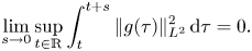
It is worth mentioning as well that if $g$ is weakly normal, then any $\xi \in \mathcal {H}(g)$
 is also weakly normal, namely, for any $\xi \in \mathcal {H}(g)$
 , there exist $\widetilde \xi _\varepsilon \in \mathcal {H}(\widetilde g_\varepsilon )$
 and $\bar \xi _\varepsilon \in \mathcal {H}(\bar g_\varepsilon )$
 such that $\xi =\widetilde \xi _\varepsilon +\bar \xi _\varepsilon$
 and the functions $\bar \xi _\varepsilon$
 satisfy (5.12) uniformly with respect to $\xi \in \mathcal {H}(g)$
 .
.
The next theorem can be considered as the main result of this section.
Theorem 5.7 Let the assumptions of theorem 5.4 hold and let also the right-hand side $g\in L^2_b(\mathbb {R},\,L^2(\Omega ))$ be weakly normal. Then the cocycle $\mathcal {S}_\xi (t)$
 associated with problem (5.4) possesses a strong uniform attractor $\mathcal {A}_{un}^s$
 which coincides with the weak uniform attractor constructed above.
Proof. According to proposition 5.3, we only need to find a (pre)compact uniformly absorbing set for the cocycle $\mathcal {S}_\xi (t)$ . We claim that the set

where $\mathcal {B}$ is defined via (5.11) is a desired absorbing set. Indeed, due to estimate (5.10) this set is absorbing and bounded, so we only need to check its compactness. Let $v_n\in \mathcal {B}_1$
 is an arbitrary sequence. Then there exists a sequence of the initial data $u_0^n\in \mathcal {B}$
 and a sequence of right-hand sides $\xi _n\in \mathcal {H}(g)$
 such that $v_n=u_n(1)$
 , where $u_n(t):=\mathcal {S}_{\xi _n}u_0^n$
 is the corresponding sequence of solutions of problem (5.4). Since $\mathcal {B}$
 and $\mathcal {H}(g)$
 are compact in a weak topology, we may assume without loss of generality that

Moreover, since the maps $(u_0,\,\xi )\to \mathcal {S}_\xi (t)u_0$ are continuous in a weak topology for every fixed $t\ge 0$
 , we conclude that $u_n(t)\rightharpoondown u(t)$
 in $\Phi$
 for every fixed $t$
 , where $u(t):=\mathcal {S}_\xi (t)u_0$
 . In particular, $v_n\rightharpoondown u(1)$
 . Therefore, we only need to verify that this convergent is actually strong.
Arguing as in the proof of corollary 4.2, we see that we only need to verify that $E(u_n(1))\to E(u(1))$ . In turn, in order to verify this convergence, we will use the energy identity (4.1) together with the trick suggested in [Reference Zelik41]. In order to avoid technicalities, we first give the proof for the particular case where $g$
 is normal and after that indicate briefly the changes which should be made to cover the general case where $g$
 is only weakly normal.
Namely, we multiply equation (5.4) for solutions $u_n$ by $Nu_n$
 , where $N$
 is a big positive constant, integrate over $x\in \Omega$
 and take a sum with (4.1) for $u_n$
 . This gives the following identity:

Multiplying this identity by $t$ and integrating over $t\in [0,\,1]$
 , we arrive at

We want to pass to the limit $n\to \infty$ in this identity. To this end, we note that by convexity arguments

To pass to the limit in the other terms, we recall that, due to estimates (3.5) and (3.45), the sequence $u_n$ is bounded in the space

and therefore, since this space is compactly embedded to $L^2(0,\,1;W^{1,2}(\Omega ))\cap L^{r+1}(0,\,1;L^{r+1}(\Omega ))$ , we have the strong convergence $u_n\to u$
 in this space. This allows us to pass to the limit in the last term in the left-hand side of (5.16) as well as in the first and the last terms in the right-hand side there. Moreover, arguing analogously to the proof of theorem 4.1 (see (4.10)), we prove that $(u_n,\,\nabla _x)u_n\to (u,\,\nabla _x)u$
 strongly in $L^2(0,\,1;L^2(\Omega ))$
 and this allows us to pass to the limit in the second term in the right-hand side of (5.16). The third term is obvious since $u_n\to u$
 strongly in $L^2(0,\,1;L^2(\Omega ))$
 and the only problem is the last term in the right-hand side. In contrast to the other terms, we have here only weak convergence $\xi _n\to \xi$
 and $\partial _t u_n\to \partial _t u$
 in $L^2(0,\,1;L^2(\Omega ))$
 and cannot use the convexity arguments. Instead, we prove that this term is small when $N$
 is large uniformly with respect to $n$
 and this will be enough for our purposes.
Lemma 5.8 Under the above assumptions, the following convergence holds:

Proof of the lemma Indeed, since $\partial _t u_n$ are uniformly bounded in the space $L^2(0,\,1;L^2(\Omega ))$
 , due to Cauchy-Schwarz inequality, we have

It only remains to recall that assumption (5.13) implies that
see [Reference Zelik41, Reference Zelik42] for the details. This finishes the proof of the lemma.
We now ready to finish the proof of the theorem for the case where $g$ is normal. Let $\varepsilon >0$
 be arbitrary. Then, due to the lemma, we may fix $N=N(\varepsilon )$
 in such a way that the last term in the right-hand side of (5.16) will be less than $\varepsilon$
 . Passing to the limit $n\to \infty$
 in (5.16) then gives

Comparing this inequality with the identity (5.16) for the limit solution $u(t)$ and using the lemma again, we end up with the inequality

Since $\varepsilon >0$ is arbitrary, passing to the limit $\varepsilon \to 0$
 gives us the inequality
The opposite inequality follows from the weak convergence $u_n(1)\to u(1)$ in $\Phi$
 and the convexity arguments. Thus, we have proved the convergence $E(u_n(1))\to E(u(1))$
 which gives us the desired strong convergence $u_n(1)\to u(1)$
 in $\Phi$
 and finishes the proof of the theorem in the case of normal external forces $g$
 .
.
Let us assume now that $g$ is weakly normal. In this case, the external forces $\xi _n$
 can be split in two parts $\widetilde \xi _{n,\varepsilon }\in L^2_b(\mathbb {R},\,H_\varepsilon )$
 , where $\varepsilon >0$
 is arbitrary and $H_\varepsilon$
 is smooth and finite-dimensional and $\bar \xi _{n,\varepsilon }$
 which satisfy (5.12) uniformly with respect to $n$
 . The analogue of (5.18) now reads

where $C$ is independent of $\xi \in \mathcal {H}(g)$
 , see [Reference Zelik41]. Therefore, as in the case of normal external forces, the term containing $(\xi _{n,\varepsilon }(s),\,\partial _t u_n(s))$
 can be made arbitrarily small by choosing $N$
 and $\varepsilon$
 big and small enough respectively. In contrast to this, the term containing $(\widetilde \xi _{n,\varepsilon }(s),\,\partial _t u_n(s))$
 cannot in general be made small and we should treat it in a different way. Namely, we introduce a corrector $v_{n,\varepsilon }(t)$
 as a solution of the following linear Stokes problem

Then, since $\widetilde \xi _{n,\varepsilon }$ are uniformly with respect to $n$
 smooth, using the anisotropic $L^2(0,\,1;L^s(\Omega ))$
 -maximal regularity estimate for the solutions of the Stokes equation, for every finite $s$
 , we have the uniform estimate

This estimate shows that, without loss of generality, we may assume that

Let $w_n:=u_n-v_{n,\varepsilon }$ . Then this function solves

We write the analogue of (5.16) for this equation by multiplying it by $t(\partial _t w_n+Nw_n)$ and integrating over $x\in \Omega$
 and time. Due to the presence of the corrector $v_{n,\varepsilon }$
 , we will have several extra terms in this equality, namely, the energy $E(u_n(t))$
 will be replaced by
From the nonlinearity $f$ , we will have an extra term which contains

This term is not dangerous since from (5.24) we have the weak convergence of $\partial _t v_{n,\varepsilon }+N v_{n,\varepsilon }$ in $L^2(0,\,1;L^s(\Omega ))$
 for all $s<\infty$
 and, arguing as above, we may check that $f(u_n)\to f(u)$
 strongly in $L^2(0,\,1;L^{1+\delta }(\Omega ))$
 for sufficiently small positive $\delta$
 . We will also have the term containing $(u_n,\,\nabla _x)u_n,\,\partial _t v_{n,\varepsilon }+Nv_{n,\varepsilon })$
 which is not dangerous as well since we have the strong convergence of $(u_n,\,\nabla _x) u_n$
 in $L^2(0,\,1;L^2(\Omega ))$
 .
.
The main advantage of this modified energy identity is that the bad term containing $(\widetilde \xi _{n,\varepsilon },\,\partial _t u_n)$ disappears and we may argue as in the case of normal external forces and verify that

Moreover, since $v_{n,\varepsilon }(1)\to v_\varepsilon (1)$ strongly in $\Phi$
 , we may replace $\widetilde E(u_n(1))$
 by $E(u_n(1))$
 in (5.26). Finally, since $E(u_n(1))$
 is independent of $\varepsilon$
 , we may pass to the limit $\varepsilon \to 0$
 and end up with inequality (5.20) in the case of weakly normal external forces as well. Then, as before, we derive the opposite inequality by the convexity arguments and finally establish that $u_n(1)\to u(1)$
 strongly in $\Phi$
 . This finishes the proof of the theorem.
Acknowledgements
This work is partially supported by Moscow Center for Fundamental and Applied Mathematics, Agreement with the Ministry of Science and Higher Education of the Russian Federation, No. 075-15-2019-1623

 Open access