


1. Introduction
Variable annuities(VAs) are a type of equity-linked insurance that offer a rich variety of embedded financial options in the form of investment guarantees. The guarantees may be very complex, and the maturities are very long, contributing to potentially significant costs arising from hedge rebalancing in discrete time. Estimating the tail risk measures of the VA liabilities, including discrete hedging costs, is of prime interest for risk management and regulatory capital assessment.
In most cases, the evaluation of these risk measures is computationally burdensome, requiring nested, path-dependent Monte Carlo simulation. Developing more efficient and accurate methods for the valuation and risk management of embedded options is a topic of considerable interest to insurers and has applications more broadly in financial risk management. In this paper, we consider the estimation of the conditional tail expectation (CTE, also known as expected shortfall) for a VA with two forms of guaranteed minimum maturity benefit, but the method can be applied to other financial options, and to other risk measures such as value at risk (VaR).
The nested simulation process for assessing the distribution of hedging costs for VAs requires two levels of simulation:
The outer level simulation projects the underlying risk factors under the real-world measure. In many finance applications, the projection involves only a single step, but in our context the outer level projections are multi-period, with the time step based on the assumed hedge rebalancing frequency. The outer level simulated paths are known as the outer scenarios, or just scenarios, and may include simulated asset returns, interest rates, policyholder behaviour and longevity experience.
The inner simulations are used to value the embedded options at each future date, conditional on the outer level scenarios up to each valuation date. As this is a valuation step, a risk-neutral pricing measure is used. Note that in this multi-period problem, the inner simulation stage is repeated, with new simulated paths, at each time step of each outer scenario.
In Figure 1, we illustrate the nested simulation process both for the single period and the multi-period case. The entire figure represents the multi-period case, while the portion circled in the green represents the single-period case.
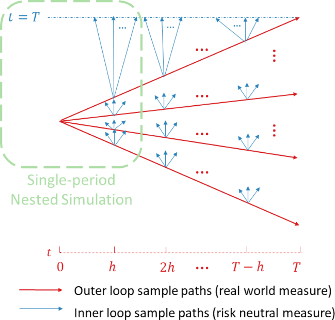
Figure 1. Nested simulation structure.
For insurers, large-scale nested simulations for assessing VA losses will take considerable run time. A large number of outer level simulations are needed in order to estimate the extreme tails needed for VaR or CTE calculations, and a large number of inner simulations are needed at each time step, because the embedded options are often far out of the money. Furthermore, the calculations have to be repeated for each VA policy, or cluster of policies, in force. Consequently, many insurers are very interested in variance reduction techniques for nested simulation models that can achieve accurate results within a limited computational budget.
Similar nested simulation challenges arise in banking, where exotic options and intractable pricing measures make the assessment of the VaR or CTE exposure too complex for analytic calculation. Holton (Reference Holton2003) points out that large-scale nested simulation is too time-consuming for practical, everyday risk analysis, where risk exposures may be required with only a few minutes notice. Compromises, such as limiting the choice of pricing models, or prematurely terminating simulations, are usually insufficiently accurate for tail risks and can produce unacceptably biased estimators.
The literature on nested simulations focuses either on an efficient allocation of computational budget between outer and inner simulations (e.g. Gordy & Juneja, Reference Gordy and Juneja2010), or on methods to improve the efficiency of inner simulations. Among the work that aims at reducing the computational burden of inner simulations, two different approaches have been proposed. The first uses proxy models to replace the inner simulation step, and the second uses a dynamic, non-uniform allocation of the inner simulations.
Proxy models are tractable analytic functions that replace the inner simulation stage of a nested simulation. Proxies may be empirical – that is, intrinsic to the simulation process, or may be extrinsic. Empirical proxies are constructed using an initial pilot simulation to develop factors or functionals that can subsequently be used in place of the inner simulation. Hardy & Wirch (Reference Hardy and Wirch2004) used a simple linear interpolation approach for calculating iterated risk measures; several authors, including Bauer & Ha (Reference Bauer and Ha2015) use a least squares Monte Carlo method (following Longstaff & Schwartz, Reference Longstaff and Schwartz2001), Risk & Ludkovski (Reference Risk and Ludkovski2018) use Gaussian Process regression, and Feng & Jing (Reference Feng and Jing2017) describe a generic partial differential equation approach. Extrinsic proxy functions are selected to be close to the inner simulation values and therefore require detailed information about the pay-offs that are evaluated using the inner simulations. See Aggarwal et al. (Reference Aggarwal, Beck, Cann, Ford, Georgescu, Morjaria, Smith, Taylor, Tsanakas, Witts and Ye2016) for other examples. Proxy methods are popular in practice, but there is a risk that the proxy may become less accurate over time, without the user becoming aware of the divergence. Rigorous backtesting can be useful in assessing the continuing suitability of a proxy, but that can be infeasible for long-term contracts. In this work, we use an extrinsic proxy, but we have revised the role played by the proxy, compared with the papers cited, and one of the consequences is that the suitability of the proxy model can be reviewed directly, without backtesting.
Methods utilising a dynamic, non-uniform allocation of the computational budget of a nested simulation have been developed by Lan et al. (Reference Lan, Nelson and Staum2010), Broadie et al. (Reference Broadie, Du and Moallemi2011) and Risk & Ludkovski (Reference Risk and Ludkovski2018). Typically, the total number of inner simulations that will be distributed across the scenarios is fixed. This is the inner simulation budget. The uniform nested simulation method allocates the inner simulation budget equally across all the scenarios. Dynamic allocation involves non-uniform allocation of the inner simulation budget. Lan et al. (Reference Lan, Nelson and Staum2010) suggest a two-stage process, with the results from a small number of initial inner simulations, uniformly allocated, being used to signal which scenarios were likely to have the most impact on the risk measure. The remainder of the inner simulation budget is then allocated only to these scenarios. Broadie et al. (Reference Broadie, Du and Moallemi2011) also use a smaller number of initial trial simulations, but their method then proceeds sequentially, determining which individual scenario should be allocated the next simulation from the remaining inner simulation budget. Risk & Ludkovski (Reference Risk and Ludkovski2018) use a trial simulation to initialise a Gaussian Process emulator as empirical proxy and then develop a k-round sequential algorithm that adaptively allocates the inner simulation budget.
Methods involving trial inner simulations do not transfer well to the VA context. VA options are typically far out of the money, so a small number of trial inner simulations will not give an adequate assessment of the hedging losses in the general case, although in some specific cases importance sampling within the inner simulations could mitigate this problem.
It is also worth noting that in each of Gordy & Juneja (Reference Gordy and Juneja2010), Broadie et al. (Reference Broadie, Du and Moallemi2011) and Risk & Ludkovski (Reference Risk and Ludkovski2018), the problem involves a single-step outer scenario, which facilitates a sequential approach, as there is only one set of inner simulations to consider for each scenario. In the multi-period problem that we are considering, typically, an insurer will project risk factors up to 20 years ahead, in weekly or monthly time steps, and new inner level simulations (which may be single or multi-period, depending on the path dependency of the embedded options) are required at each time step of each scenario, as illustrated in Figure 1. The main challenge in applying the methods developed for single-period nested simulation to the multi-period problem is the multiplicative increase in the dimension of the problem being considered. When conducting pilot simulations, a significant amount of computation may be required to produce any meaningful signal as to which scenarios belong to the tail. When applying regression techniques, if we try to apply single-step methods directly, the dimension of the multi-period problem will be hundreds of times the size of the single-period problem.
In this paper, we introduce a dynamic importance allocated nested simulation (DIANS) methodology, which is an extension of the IANS method introduced in Dang et al. (Reference Dang, Feng and Hardy2020). The method combines elements of the proxy model approach with elements of the dynamic allocation approach. More specifically, DIANS uses a proxy model to indicate which scenarios are likely to generate the most significant losses and then allocates the entire inner simulation budget to that subset of scenarios. Our proxy model takes on the role of the initial trial simulations in Lan et al. (Reference Lan, Nelson and Staum2010) and Risk & Ludkovski (Reference Risk and Ludkovski2018), but without using any of the inner simulation budget. The proxy model values are not used directly in the estimation of the risk measure, and they are only used to determine the allocation of the inner simulation budget. Hence, the proxy model does not have to provide an accurate valuation of the underlying losses; it only has to provide a reasonably accurate ranking of the values of the underlying losses. Because the rankings generated by the proxy will not exactly match the underlying ranking, we apply a margin to allow for the difference between the rankings generated by the proxy model and more accurate rankings generated by inner simulation. In the IANS method, this margin is fixed and arbitrary. The contribution of this paper is to remove that arbitrary margin and replace it with a dynamic algorithm, based on the relationship between the proxy model and inner simulation rankings for a trial subset of scenarios; if the relationship is not sufficiently close, the subset of scenarios assigned to the tail set is increased iteratively. The closeness of rankings is measured using the empirical copula to generate moments of concomitant of order statistics (David, Reference David1973) for the proxy model in relation to the inner simulation model. The dynamic methodology not only reduces the need for subjective input, it also provides a measure for assessing the performance of the extrinsic proxy. If the iterative process indicates a need to incorporate a very large number of scenarios into the tail set, that signals that the proxy is not performing adequately, reducing the reliance on backtesting.
We note that our work is concerned with the efficient estimation of risk measures for a single policy. In practice, VA portfolios may include hundreds of thousands of contracts with different demographic profiles. This very large number of model points generates a need for a different kind of efficiency, reducing the reliance on seriatim policy valuation. Other research has considered this issue, combined with methods for estimating the losses on a large heterogeneous portfolio. Gan & Valdez (Reference Gan and Valdez2019) present various metamodelling approaches to select representative policies and use functional approximations to predict the values of the entire portfolio. Lin & Yang (Reference Lin and Yang2020b, a) also consider nested simulation of a large portfolio, Lin & Yang (Reference Lin and Yang2020b) in the single-period and Lin & Yang (Reference Lin and Yang2020a) in the multi-period setting. They use a cube sampling algorithm to select representative policies and use clustering to select representative outer scenarios. Functional approximations are then used to predict the value of the liabilities. Their work demonstrates a significant computational saving, but the larger impact (around 98
 $\%$
of the computational saving) is achieved by reducing the number of model points, through the use of representative policies. This paper has a different focus; we are concerned with improving the estimation of the tail measures efficiently, for a given representative policy.
$\%$
of the computational saving) is achieved by reducing the number of model points, through the use of representative policies. This paper has a different focus; we are concerned with improving the estimation of the tail measures efficiently, for a given representative policy.
The paper is structured as follows. Section 2 describes how the liability of a VA contract with dynamic hedging is modelled using a standard, multi-period nested simulation, with uniform allocation of the inner simulation budget to all the scenarios. Section 3 presents the DIANS procedure. In section 4, we illustrate the methodology using two types of VA guarantees to demonstrate the potential improvement in computational efficiency by using the DIANS procedure. Section 5 concludes the paper.
2. Uniform Nested Simulation for Variable Annuity Hedge Costs
2.1 Dynamic hedging for variable annuities via nested simulation
In this section, we present the methodology for a generic VA liability. In section 4, we describe the more specific assumptions used for numerical illustrations. The description here is similar to that in Dang et al. (Reference Dang, Feng and Hardy2020), but we have extended the notation to allow for the extension to a dynamic methodology. For more information on VA contracts and different types of guarantees, see for example Hardy (Reference Hardy2003).
In a dynamic hedging programme, a hedging portfolio is set up for a block of VA contracts using stocks, bonds, futures and possibly options. The hedging portfolio is rebalanced periodically, responding to changes in market conditions and in the demographics of the block of contracts. In this paper, we consider a delta hedge for a single VA contract.
We assume the term of the VA is T years, and the hedging portfolio is rebalanced every h years; h is also the size of time step for the outer level scenarios.
Let
 $\omega_i(t)$
denote the ith outer level scenario information up to time t;
$\omega_i(t)$
denote the ith outer level scenario information up to time t;
 $\omega_i(T)=\omega_i$
.
$\omega_i(T)=\omega_i$
.
At any
 $t\leq T$
, let
$t\leq T$
, let
 $S_i(t)$
be the underlying stock price at time t in outer scenario i. We assume that the delta hedge for the embedded option is composed of
$S_i(t)$
be the underlying stock price at time t in outer scenario i. We assume that the delta hedge for the embedded option is composed of
 $\Delta_i(t)$
units in the underlying stock, and a sum
$\Delta_i(t)$
units in the underlying stock, and a sum
 $B_i(t)$
in a risk-free zero coupon bond maturing at T. The delta hedge portfolio at
$B_i(t)$
in a risk-free zero coupon bond maturing at T. The delta hedge portfolio at
 $t-h$
is then,
$t-h$
is then,
 \begin{equation*}H_i(t-h)=\Delta_i(t-h)S_i(t-h)+B_i(t-h)\end{equation*}
Let
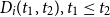 $D_i(t_1, t_2), t_1\leq t_2$
be the present value at
$D_i(t_1, t_2), t_1\leq t_2$
be the present value at
 $t_1$
of
$t_1$
of
 $\$1$
payable at time
$\$1$
payable at time
 $t_2$
, discounted at the risk-free rate. At time t, before rebalancing, the value of the hedge brought forward from
$t_2$
, discounted at the risk-free rate. At time t, before rebalancing, the value of the hedge brought forward from
 $t-h$
is
$t-h$
is
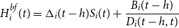 \begin{align} H^{bf}_i(t)=\Delta_i(t-h)S_i(t)+\frac{B_i(t-h)}{D_i(t-h, t)}\end{align}
The cash flow incurred by the insurer, which we call the hedging error, is the difference between the cost of the hedge at t and the value at t of the hedge brought forward from
 $t-h$
:
$t-h$
:
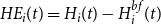 \begin{equation} \textit{HE}_i(t) =H_i(t) - H^{bf}_i(t)\end{equation}
We assume management fees are deducted from policyholder’s fund at a gross rate of
 $\eta^g$
per h years, and that a portion equal to
$\eta^g$
per h years, and that a portion equal to
 $(1 - \frac{\eta^n}{\eta^g})$
is used to cover expenses, so that the insurer’s income from fees is received at at a net rate of
$(1 - \frac{\eta^n}{\eta^g})$
is used to cover expenses, so that the insurer’s income from fees is received at at a net rate of
 $\eta^n$
per h years.
$\eta^n$
per h years.
The costs to set up the initial hedging portfolio, the periodic hedging gains and losses due to rebalancing at each date,
 $t=h, 2h, ..., T$
, the final unwinding of the hedge, the payment of guaranteed benefit and the management fee income, are recognised as part of the profit and loss (P&L) of the VA contract. The present value of these cash flows, discounted at the risk-free rate of interest, constitutes the liability of the VA to insurers; this is the loss random variable to which we apply a suitable risk measure.
$t=h, 2h, ..., T$
, the final unwinding of the hedge, the payment of guaranteed benefit and the management fee income, are recognised as part of the profit and loss (P&L) of the VA contract. The present value of these cash flows, discounted at the risk-free rate of interest, constitutes the liability of the VA to insurers; this is the loss random variable to which we apply a suitable risk measure.
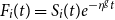
For a guaranteed minimum maturity benefit (GMMB) the guaranteed payout at T is a fixed sum G, and the liability can be decomposed as follows. Let
 $F_i(t)$
denote the value of the policyholder’s funds at t. The funds increase in proportion to a stock index with value
$F_i(t)$
denote the value of the policyholder’s funds at t. The funds increase in proportion to a stock index with value
 $S_i(t)$
at t, net of the gross management fee deduction. Let
$S_i(t)$
at t, net of the gross management fee deduction. Let
 $F(0)=S(0)$
, then
$F(0)=S(0)$
, then
 ${F_i(t) = S_i(t) e^{-\eta^g t}}$
. The cost of the initial hedge is
${F_i(t) = S_i(t) e^{-\eta^g t}}$
. The cost of the initial hedge is
 ${H(0)=\Delta(0)S(0)+B(0)}$
, which does not depend on
${H(0)=\Delta(0)S(0)+B(0)}$
, which does not depend on
 $\omega_i$
. The random loss generated by the ith scenario,
$\omega_i$
. The random loss generated by the ith scenario,
 $L_i$
, is
$L_i$
, is
 \begin{align}L_i=&H(0)+\sum_{k=1}^{T/h-1} \left(H\!E_i(kh) - (e^{\eta^n}-1)F_i(kh)\right)\,D(0,kh) +\left((G-F_i(T))^+ -H^{bf}_i(T)\right)D(0,T) \end{align}
For a guaranteed minimum accumulation benefit (GMAB) the guaranteed payout involves two dates: the renewal date,
 $T_1$
, and the maturity date,
$T_1$
, and the maturity date,
 $T>T_1$
. Let
$T>T_1$
. Let
 $G_i(t)$
denote the guarantee value at t, under scenario i. We assume that
$G_i(t)$
denote the guarantee value at t, under scenario i. We assume that
 $G_i(0)=F(0)$
(i.e. the initial guarantee is equal to the initial investment). At time
$G_i(0)=F(0)$
(i.e. the initial guarantee is equal to the initial investment). At time
 $T_1$
, if the fund value is less than
$T_1$
, if the fund value is less than
 $G_i(0)$
, then the insurer pays the difference into the fund. If the fund value is greater than theinitial guarantee, then the guarantee reset to be equal to the fund value. The random loss generated by the ith scenario,
$G_i(0)$
, then the insurer pays the difference into the fund. If the fund value is greater than theinitial guarantee, then the guarantee reset to be equal to the fund value. The random loss generated by the ith scenario,
 $L_i$
, is
$L_i$
, is
 \begin{align}L_i=&H(0)+\sum_{k=1}^{T/h-1} \left(H\!E_i(kh) - (e^{\eta^n}-1)F_i(kh)\right)\,D(0,kh)+\left((G_i(T)-F_i(T))^+ -H^{bf}_i(T)\right)D(0,T) \end{align}
where the pay-off at
 $T_1$
, if any, is captured in
$T_1$
, if any, is captured in
 $H\!E_i(T_1)$
, and
$H\!E_i(T_1)$
, and
 $G_i(T)=\max(F_i(0),F_i(T_1))$
.
$G_i(T)=\max(F_i(0),F_i(T_1))$
.
 $\widehat{L}_i$
represents the estimated value of
$\widehat{L}_i$
represents the estimated value of
 $L_i$
based on the inner simulations.
$L_i$
based on the inner simulations.
The risk measure of interest is the
 $\alpha$
-CTE (Wirch & Hardy, Reference Wirch and Hardy1999), which is the expected loss given that the loss lies in the
$\alpha$
-CTE (Wirch & Hardy, Reference Wirch and Hardy1999), which is the expected loss given that the loss lies in the
 $1{-}\alpha$
tail of the distribution. This is also known as TailVar (Artzner et al., Reference Artzner, Delbaen, Eber and Heath1999) and expected shortfall (Acerbi & Tasche, Reference Acerbi and Tasche2002).
$1{-}\alpha$
tail of the distribution. This is also known as TailVar (Artzner et al., Reference Artzner, Delbaen, Eber and Heath1999) and expected shortfall (Acerbi & Tasche, Reference Acerbi and Tasche2002).
Given M equally likely scenarios, with associated losses
 $\widehat{L}_1,\ldots,\widehat{L}_M$
, the empirical
$\widehat{L}_1,\ldots,\widehat{L}_M$
, the empirical
 $\alpha$
-CTE is
$\alpha$
-CTE is
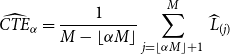 \begin{equation}\widehat{{CTE}}_{\alpha}={\frac{1}{M-\lfloor \alpha M\rfloor}\sum_{j=\lfloor \alpha M\rfloor+1}^M\,\widehat{L}_{(j)}}\end{equation}
where
 $\widehat{L}_{(j)}$
is the jth smallest loss value, or jth order statistic, of the M simulated values. To simplify the notation, we assume that
$\widehat{L}_{(j)}$
is the jth smallest loss value, or jth order statistic, of the M simulated values. To simplify the notation, we assume that
 $\alpha M$
is an integer hereinafter. In practice, the number of outer scenarios is generally large enough to satisfy this assumption.
$\alpha M$
is an integer hereinafter. In practice, the number of outer scenarios is generally large enough to satisfy this assumption.
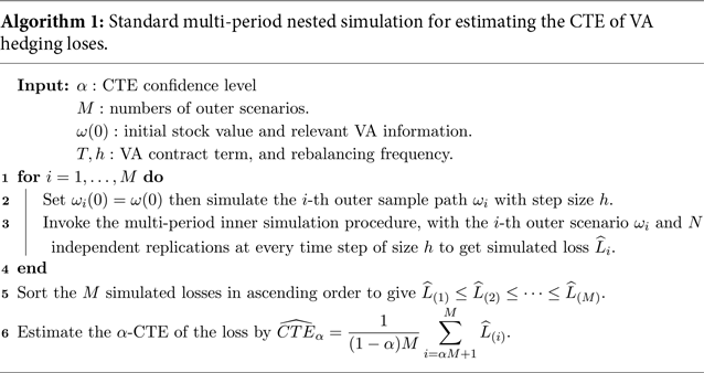
2.2 Multi-period uniform nested simulation
A typical multi-period nested simulation procedure used to estimate the
 $\alpha$
-CTE is described in Algorithm 1. The outer simulation in Line 2 projects the underlying stock price under the real-world measure for K time steps, along with other variables such as lapses and, potentially, interest rates. The multi-period inner simulation procedure is invoked with N independent replications at each of the K time steps of each of the M outer scenarios.
$\alpha$
-CTE is described in Algorithm 1. The outer simulation in Line 2 projects the underlying stock price under the real-world measure for K time steps, along with other variables such as lapses and, potentially, interest rates. The multi-period inner simulation procedure is invoked with N independent replications at each of the K time steps of each of the M outer scenarios.
The hedge costs at each rebalancing time will depend on the hedging strategy. In our numerical illustrations, the relevant Greeks are estimated using the infinite perturbation analysis (IPA) method, also known as the pathwise method, (Broadie & Glasserman, Reference Broadie and Glasserman1996; Glasserman, Reference Glasserman2013). Other methods for the computation of Greeks, such as the likelihood ratio method (L’Ecuyer, Reference L’Ecuyer1990) or simultaneous perturbation (Fu et al., Reference Fu2015), give similar results.
We refer to the total number of inner simulation replications, for each time step, as the simulation budget and denote it by
 $\Gamma$
. For example, the simulation budget in Algorithm 1 is
$\Gamma$
. For example, the simulation budget in Algorithm 1 is
 $\Gamma= M\times N$
. We assume that the required number of outer scenarios (M) is fixed; our objective (similarly to Gordy & Juneja, Reference Gordy and Juneja2008; Broadie et al., Reference Broadie, Du and Moallemi2011 and Risk & Ludkovski, Reference Risk and Ludkovski2018) will be to improve accuracy through a non-uniform allocation of the inner simulation budget. Note that the actual computational budget associated with N inner simulations is greater than
$\Gamma= M\times N$
. We assume that the required number of outer scenarios (M) is fixed; our objective (similarly to Gordy & Juneja, Reference Gordy and Juneja2008; Broadie et al., Reference Broadie, Du and Moallemi2011 and Risk & Ludkovski, Reference Risk and Ludkovski2018) will be to improve accuracy through a non-uniform allocation of the inner simulation budget. Note that the actual computational budget associated with N inner simulations is greater than
 $M\times N$
, as we use a new set of N simulations at each time step of each scenario.
$M\times N$
, as we use a new set of N simulations at each time step of each scenario.
Given the M outer scenarios, the true m-tail scenario set, denoted
 $\mathcal{T}_m$
, is the subset containing the m scenarios associated with the largest losses. That is,
$\mathcal{T}_m$
, is the subset containing the m scenarios associated with the largest losses. That is,
 \begin{equation}\mathcal{T}_m = \left\{\omega_i\,:\, L_i > L_{(M-m)}\right\}\end{equation}
where
 $L_i$
is the (unknown) true hedge loss associated with scenario
$L_i$
is the (unknown) true hedge loss associated with scenario
 $\omega_i$
, for
$\omega_i$
, for
 $i=1,\ldots,M$
, and
$i=1,\ldots,M$
, and
 $L_{(j)}$
is the jth smallest value of the
$L_{(j)}$
is the jth smallest value of the
 $L_i$
’s.
$L_i$
’s.
3. Dynamic Importance Allocated Nested Simulation (DIANS)
The DIANS method exploits the fact that the CTE calculation only uses the largest
 $(1{-}\alpha)M$
simulated loss values, so the inner simulation budget can be concentrated on the scenarios which are most likely to generate the largest losses. We use a proxy model to determine these scenarios.
$(1{-}\alpha)M$
simulated loss values, so the inner simulation budget can be concentrated on the scenarios which are most likely to generate the largest losses. We use a proxy model to determine these scenarios.
To identify a suitable proxy model, we first consider why the inner simulation step is needed. Typically, the complexity in the valuation, leading to the need for the guarantee cost to be determined using simulation rather than analytically, comes from some combination of the following issues.
-
(1) An intractable risk-neutral measure; this is a common problem, as the contracts are very long term, and models used often involve stochastic volatility, for which analytic valuation formulae may not be available.
-
(2) Dynamic lapse assumptions; insurers typically assume that lapses are (somewhat) dependent on the moneyness of the guarantee. A popular version of the dynamic lapse model, from the National Association of Insurance Commissioners (NAIC, 2019), is described in section 4.1. Incorporating dynamic lapses creates a path-dependent option valuation that is not analytically tractable.
-
(3) The option pay-off is too complex for analytic valuation.
The proxy model should be a tractable model that is close enough to the more complex model to give an approximate ranking of the scenarios. We might construct the proxy by using a tractable risk-neutral measure in place of the stochastic volatility model, to cover issue (1) above; we might use a simplified lapse rate assumption, to deal with issue (2) above, and we might replace a complex pay-off with a simpler one that captures most of the costs to cover issue (3) above. We reiterate that the proxy does not have to give an accurate estimate of the option costs based on the more complex assumptions; it is sufficient that the scenarios generating the highest losses under the proxy model overlap significantly with the scenarios generating the highest losses under the full inner simulation approach.
In cases where no obvious extrinsic proxy model is available, an intrinsic proxy can be constructed from PDEs (see Feng, Reference Feng2014), or by applying likelihood ratio estimators based on a pilot simulation. The intrinsic proxy only needs to be accurate enough to separate tail scenarios from the rest of the scenarios, in terms of overall losses. The selection of the proxy model should also consider the computation cost trade-off. For example, suppose that proxy model A can rank the scenarios more accurately than proxy model B, but at much greater computational cost. It may be more efficient to use proxy model B, and increase the inner simulation budget, than to run model A with the smaller inner simulation budget. The key to a successful proxy model is to ensure that the computation cost required in running the proxy model is justified compared to the computation cost saved by avoiding in inner simulation of non-tail scenarios.
The proxy model is used to identify a set of scenarios that is likely to contain the scenarios associated with the largest losses. Let
 $L^P_i$
denote the loss, based on the proxy model, given scenario
$L^P_i$
denote the loss, based on the proxy model, given scenario
 $\omega_i$
,
$\omega_i$
,
 $i=1,2,\ldots,M$
. Let
$i=1,2,\ldots,M$
. Let
 $L^P_{(j)}$
denote the jth ranked value of
$L^P_{(j)}$
denote the jth ranked value of
 $L^P_i$
. Then the proxy tail scenario set with m scenarios is denoted
$L^P_i$
. Then the proxy tail scenario set with m scenarios is denoted
 $\mathcal{T}^P_{m}$
, where
$\mathcal{T}^P_{m}$
, where
 \begin{equation*}\omega_i \in \mathcal{T}^P_{m} \Leftrightarrow L^P_i > L^P_{(M-m)}\end{equation*}
In other words, a scenario is in the proxy tail scenario set,
 $\mathcal{T}^P_{m}$
, if the proxy loss associated with that scenario is one of the largest m losses out of the full set of M losses.
$\mathcal{T}^P_{m}$
, if the proxy loss associated with that scenario is one of the largest m losses out of the full set of M losses.
We want the proxy tail scenario set to overlap with the
 $(1-\alpha)M$
true tail scenario set used in the
$(1-\alpha)M$
true tail scenario set used in the
 $\alpha$
-CTE (given the M scenarios),
$\alpha$
-CTE (given the M scenarios),
 $\mathcal{T}_{(1-\alpha)M}$
. We select
$\mathcal{T}_{(1-\alpha)M}$
. We select
 $m \geq (1-\alpha)M$
proxy tail scenarios such that we can be confident that few or no scenarios are in
$m \geq (1-\alpha)M$
proxy tail scenarios such that we can be confident that few or no scenarios are in
 $\mathcal{T}_{(1-\alpha)M}$
but not in
$\mathcal{T}_{(1-\alpha)M}$
but not in
 $\mathcal{T}^P_{m}$
. Once we have
$\mathcal{T}^P_{m}$
. Once we have
 $\mathcal{T}^P_{m}$
, the inner simulation budget is allocated, in full and uniformly, to the scenarios in
$\mathcal{T}^P_{m}$
, the inner simulation budget is allocated, in full and uniformly, to the scenarios in
 $\mathcal{T}^P_{m}$
, with no further estimation of losses for other scenarios. The estimated loss for
$\mathcal{T}^P_{m}$
, with no further estimation of losses for other scenarios. The estimated loss for
 $\omega_i \in \mathcal{T}^P_{m}$
is
$\omega_i \in \mathcal{T}^P_{m}$
is
 $^m\widehat{L}_i$
, and these are sorted into the sequence
$^m\widehat{L}_i$
, and these are sorted into the sequence
 $^m\widehat{L}_{(j)}$
, for
$^m\widehat{L}_{(j)}$
, for
 $j=1,2,\ldots,m$
. The estimated CTE is then
$j=1,2,\ldots,m$
. The estimated CTE is then
 \begin{equation}\widehat{CTE}_{\alpha}=\frac{1}{(1-\alpha)M}\sum_{j=m-(1-\alpha)M+1}^m \!\!\!\!{}^m\widehat{L}_{(j)}\end{equation}
The problem here is that in order to capture the largest
 $(1-\alpha)M$
true tail scenarios, we need more than
$(1-\alpha)M$
true tail scenarios, we need more than
 $(1-\alpha)M$
proxy tail scenarios. If we use
$(1-\alpha)M$
proxy tail scenarios. If we use
 $m\gg (1-\alpha)M$
, then we are more likely to capture the true tail scenarios, but with the inner simulation budget spread more widely, so the individual loss estimates are less accurate. If we choose a smaller value for m, then we risk missing some of the true tail scenarios, as the proxy rankings will not usually perfectly coincide with the true rankings.
$m\gg (1-\alpha)M$
, then we are more likely to capture the true tail scenarios, but with the inner simulation budget spread more widely, so the individual loss estimates are less accurate. If we choose a smaller value for m, then we risk missing some of the true tail scenarios, as the proxy rankings will not usually perfectly coincide with the true rankings.
In Dang et al. (Reference Dang, Feng and Hardy2020) a fixed, arbitrary value of
 $m=(1-\alpha+0.05)M$
was used. In this paper, we use a dynamic method to determine m, based on the emerging closeness of the ranking of losses from the proxy model and the ranking of losses from an initial set of inner simulations. This closeness is quantified using results from order statistics described in the following section.
$m=(1-\alpha+0.05)M$
was used. In this paper, we use a dynamic method to determine m, based on the emerging closeness of the ranking of losses from the proxy model and the ranking of losses from an initial set of inner simulations. This closeness is quantified using results from order statistics described in the following section.
3.1 Dynamic selection of proxy tail scenarios for DIANS
The proxyis successful if the ranking of scenarios based on the proxy model corresponds closely with the true ranking of the scenarios, which we estimate using simulation. A natural way to explore how close the rankings are is through the empirical copulas of the bivariate random variables comprised of the proxy loss and the simulated loss.
Consider the bivariate random variable
 $(L^P_i,\,L_i)$
, representing the proxy loss and the random loss generated by the ith scenarios, for
$(L^P_i,\,L_i)$
, representing the proxy loss and the random loss generated by the ith scenarios, for
 $\omega_i \in \mathcal{T}^P_m$
. Let
$\omega_i \in \mathcal{T}^P_m$
. Let
 $(U^P_i, {U}_i)$
represent the uniform random variables generated by applying the marginal distribution functions to
$(U^P_i, {U}_i)$
represent the uniform random variables generated by applying the marginal distribution functions to
 $L_i^P$
and
$L_i^P$
and
 $L_i$
, that is
$L_i$
, that is
 \begin{equation*}\left(U_i^P,\,U_i\right)=\Big(F_{L^P}\left(L^P_i\right),\,(F_{L}\left(L_i\right)\Big)\end{equation*}
We assume, for convenience, that the losses are continuous; it is straightforward to adapt the method for mixed distributions. We order the m pairs of
 $(U^P_i, {U}_i)$
by the
$(U^P_i, {U}_i)$
by the
 $U_i^P $
values, from smallest to largest, giving us the ordered sample:
$U_i^P $
values, from smallest to largest, giving us the ordered sample:
 \begin{align*}&\left(U^P_{\left(1\right)},\,U_{[1]}\right),\, \left(U^P_{\left(2\right)},\,U_{[2]}\right),\,\ldots,\left(U^P_{\left(m\right)},\,U_{[m]}\right)\end{align*}
where
 $U^P_{(j)}$
is the j-th smallest (or j-th order statistic) of the
$U^P_{(j)}$
is the j-th smallest (or j-th order statistic) of the
 $U^P_i$
values, and
$U^P_i$
values, and
 $U_{[j]}$
is known as the concomitant of the jth order statistic (David, Reference David1973).
$U_{[j]}$
is known as the concomitant of the jth order statistic (David, Reference David1973).
Let
 $R_{j\,:\,m}$
denote the rank of the value of
$R_{j\,:\,m}$
denote the rank of the value of
 $U_i$
corresponding to the jth smallest value in a sample of m values of
$U_i$
corresponding to the jth smallest value in a sample of m values of
 $U^P_i$
(or equivalently, the rank of the value of
$U^P_i$
(or equivalently, the rank of the value of
 $L_i$
corresponding to the jth smallest value of
$L_i$
corresponding to the jth smallest value of
 $L^P_i$
). Then, we have
$L^P_i$
). Then, we have
 \begin{equation*}\left(U^P_{(j)},\,U_{[j]}\right)= \left(U^P_{(j)},\,U_{(R_{j\,:\,m})}\right)\end{equation*}
If
 $U^P$
and U are comonotonic, then
$U^P$
and U are comonotonic, then
 $R_{j\,:\,m}=j$
, and we have a perfect proxy in terms of ranking of losses. If not, then we can use results from David et al. (Reference David, O’Connell and Yang1977) and O’Connell (Reference O’Connell1974) to derive formulae for moments of
$R_{j\,:\,m}=j$
, and we have a perfect proxy in terms of ranking of losses. If not, then we can use results from David et al. (Reference David, O’Connell and Yang1977) and O’Connell (Reference O’Connell1974) to derive formulae for moments of
 $R_{j\,:\,m}$
, in terms of the copula function and the copula density function of
$R_{j\,:\,m}$
, in terms of the copula function and the copula density function of
 $U^P$
and U, denoted
$U^P$
and U, denoted
 $C(u^P,u)$
and
$C(u^P,u)$
and
 $c(u^P,u),$
respectively. We also need the density function of the rth order statistic among an i.i.d. sample of m Uniform(0,1) random variables, which is
$c(u^P,u),$
respectively. We also need the density function of the rth order statistic among an i.i.d. sample of m Uniform(0,1) random variables, which is
 \begin{equation*}f_{j\,:\,m}(u) = \frac{m!}{(j-1)!(m-j)!} u^{j-1}(1-u)^{m-j}.\end{equation*}
Proposition 3.1. Let U and V denote U(0,1) random variables, with joint distribution function C(U,V) and joint density function c(u,v). Let
 $R_{j\,:\,m}$
denote the rank of the concomitant of the jth order statistic of U, from a random sample of size m, and let
$R_{j\,:\,m}$
denote the rank of the concomitant of the jth order statistic of U, from a random sample of size m, and let
 $f_{j\,:\,m}$
denote the density function defined above.
$f_{j\,:\,m}$
denote the density function defined above.
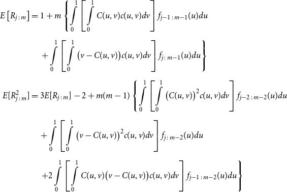 \begin{align*} E\left[R_{j\,:\,m}\right] & = 1 + m \left\{\int\limits_0^1 \left[ \int\limits_0^1 C(u,v) c(u,v) dv\right]f_{j-1\,:\,m-1}(u)du \right.\\[4pt]& \quad \left. + \int\limits_0^1 \left[\int\limits_0^1 \big(v - C(u,v)\big) c(u,v) dv\right] f_{{j\,:\,m{-}1}}(u)du\right\} \\[4pt] E[R_{j\,:\,m}^2] & = 3 E[R_{j\,:\,m}] - 2 + m(m-1) \left\{\int\limits_0^1 \left[\int\limits_0^1 \big(C(u,v)\big)^2 c(u,v) dv\right]f_{j-2\,:\,m-2}(u)du \right. \\[4pt] & \quad + \int\limits_0^1 \left[\int\limits_0^1 \big(v - C(u,v)\big)^2 c(u,v) dv\right]f_{{j\,:\,m{-}2}}(u)du \\[4pt] & \quad \left. + 2 \int\limits_0^1 \left[\int\limits_0^1 C(u,v)\big(v - C(u,v)\big) c(u,v) dv\right]f_{j {-} 1\,:\,m-2}(u)du \right\} \nonumber\end{align*}
The proof of Proposition 3.1 is shown in Appendix A.
We use this proposition to quantify how well the proxy works at ranking the losses. First, we set an initial value for the number of proxy tail scenarios, denoted
 $m_0$
. We allocate a portion of the inner simulation budget to run, say,
$m_0$
. We allocate a portion of the inner simulation budget to run, say,
 $N_0$
inner simulations for each scenario in
$N_0$
inner simulations for each scenario in
 $\mathcal{T}^P_{m_0}$
. We then assess the closeness of the ranking of proxy losses and simulated losses for scenarios in
$\mathcal{T}^P_{m_0}$
. We then assess the closeness of the ranking of proxy losses and simulated losses for scenarios in
 $\mathcal{T}^P_{m_0}$
, using the moments of rank of the concomitant for a specific order statistic. If the test (described below) is not satisfied, then we increase the number of scenarios in the set and apply
$\mathcal{T}^P_{m_0}$
, using the moments of rank of the concomitant for a specific order statistic. If the test (described below) is not satisfied, then we increase the number of scenarios in the set and apply
 $N_0$
inner simulations to the newly added proxy tail scenarios. If the proxy is working, our process will cease after a few iterations, and the remaining inner simulation budget is applied to the final proxy tail scenario set
$N_0$
inner simulations to the newly added proxy tail scenarios. If the proxy is working, our process will cease after a few iterations, and the remaining inner simulation budget is applied to the final proxy tail scenario set
 $\mathcal{T}^P_{\widetilde{m}}$
. If the iterations continue, creating tail scenario sets that are larger than a prescribed maximum, this will signal that the proxy is inadequate.
$\mathcal{T}^P_{\widetilde{m}}$
. If the iterations continue, creating tail scenario sets that are larger than a prescribed maximum, this will signal that the proxy is inadequate.
The test for increasing the sample size, or not, at each iteration proceeds as follows. Assume that there are
 $m_k$
scenarios in the proxy tail scenario set on the kth iteration. We have preliminary inner simulation results for each scenario, from which we can construct the empirical copula and copula density functions.
$m_k$
scenarios in the proxy tail scenario set on the kth iteration. We have preliminary inner simulation results for each scenario, from which we can construct the empirical copula and copula density functions.
From these, we can calculate the mean and standard deviation of the rank of a simulated loss concomitant to any given ranked proxy loss. We choose to consider the
 $d=m_0-(1-\alpha)M$
th ranked proxy loss (this value stays the same through the iterations of
$d=m_0-(1-\alpha)M$
th ranked proxy loss (this value stays the same through the iterations of
 $m_k$
). For the initial iteration of the process, the number of scenarios in the tail scenario set is
$m_k$
). For the initial iteration of the process, the number of scenarios in the tail scenario set is
 $m_0=(1-\alpha)M+d$
, so d represents the additional scenarios included beyond the minimum of
$m_0=(1-\alpha)M+d$
, so d represents the additional scenarios included beyond the minimum of
 $(1-\alpha)M$
in the initial iteration.
$(1-\alpha)M$
in the initial iteration.
We use the mean and standard deviation of the rank of concomitant of the dth ranked proxy loss to calculate a one-sided upper 95
 $\%$
bound for the concomitant rank:
$\%$
bound for the concomitant rank:
 \begin{align}{b_k= E\left[R_{d:m_k}\right]+1.645 \sqrt{V\left[R_{d:m_k}\right]}}\end{align}
If this upper bound is greater than
 $m_k-(1-\alpha)M$
, then we increase the sample size, to
$m_k-(1-\alpha)M$
, then we increase the sample size, to
 ${m_{k+1}=(1-\alpha)M+b_k}$
, and repeat the test.
${m_{k+1}=(1-\alpha)M+b_k}$
, and repeat the test.
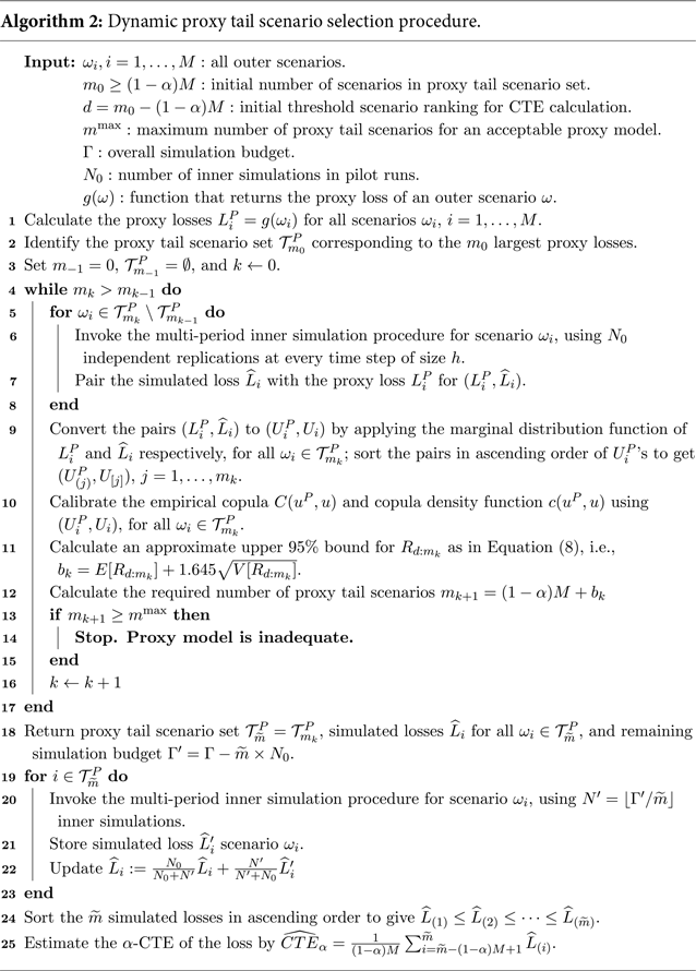
Algorithm 2 describes the process.
The choice of
 $d=m_0-(1-\alpha)M$
in the test for adequacy of
$d=m_0-(1-\alpha)M$
in the test for adequacy of
 $\mathcal{T}^P_{m_k} $
is a convenient heuristic. Intuitively (assuming positive correlation between proxy and true losses), we might prefer to use the lowest available order statistic (the minimum for which the mean and variance of the rank of the concomitant can be calculated is
$\mathcal{T}^P_{m_k} $
is a convenient heuristic. Intuitively (assuming positive correlation between proxy and true losses), we might prefer to use the lowest available order statistic (the minimum for which the mean and variance of the rank of the concomitant can be calculated is
 $d=3$
), but this will be more unstable due to the higher uncertainty at the boundary of the empirical copula. In the numerical experiments illustrated in section 4, we chose
$d=3$
), but this will be more unstable due to the higher uncertainty at the boundary of the empirical copula. In the numerical experiments illustrated in section 4, we chose
 $d = 150$
.
$d = 150$
.
The initial number of inner simulations,
 $N_0$
, is a design variable that needs to be chosen carefully. If
$N_0$
, is a design variable that needs to be chosen carefully. If
 $N_0$
is too low, then the simulated losses will be subject to greater sampling variability, leading to greater variability in
$N_0$
is too low, then the simulated losses will be subject to greater sampling variability, leading to greater variability in
 $R_{j\,:\,m}$
. This will tend to generate a higher number of tail scenarios (
$R_{j\,:\,m}$
. This will tend to generate a higher number of tail scenarios (
 $m_k$
), which is wasteful of the inner simulation budget. On the other hand, if
$m_k$
), which is wasteful of the inner simulation budget. On the other hand, if
 $N_0$
is too high, then we may run out of computation budget. One approach is to set
$N_0$
is too high, then we may run out of computation budget. One approach is to set
 $N_0$
to be the minimum number of inner simulations required for an adequate assessment of the losses, which will depend on the nature and moneyness of the embedded option.
$N_0$
to be the minimum number of inner simulations required for an adequate assessment of the losses, which will depend on the nature and moneyness of the embedded option.
Note from Line 14 of the algorithm that it may stop without calculating the CTE, if the number of proxy tail scenarios selected exceeds
 $m^{\max}$
. A valuable feature of the algorithm is that it signals when the proxy and the simulated losses have diverged such that the number of proxy tail scenarios required to capture the true tail scenarios would be too large, in the sense that the inner simulation budget would be spread too thinly for adequate accuracy of the tail risk measure estimate. An example is shown in the following section. Setting
$m^{\max}$
. A valuable feature of the algorithm is that it signals when the proxy and the simulated losses have diverged such that the number of proxy tail scenarios required to capture the true tail scenarios would be too large, in the sense that the inner simulation budget would be spread too thinly for adequate accuracy of the tail risk measure estimate. An example is shown in the following section. Setting
 $m^{\max}=M$
removes the stopping point so that, if necessary, the algorithm continues until all M scenarios are included in the inner simulation set. In this case, the DIANS procedure becomes a standard nested simulation.
$m^{\max}=M$
removes the stopping point so that, if necessary, the algorithm continues until all M scenarios are included in the inner simulation set. In this case, the DIANS procedure becomes a standard nested simulation.
Another useful feature of the algorithm is that each round of iteration provides the sample size for the next round. Even though statistics such as Spearman’s rho or Kendall’s tau also give an indication of the level of rank dependency, they provide no guidance on the sample size increment, nor do they offer any objective criteria for when the iteration could stop.
The algorithm specifically targets the
 $\alpha$
-CTE estimate, but it can be easily adapted to other tail risk measures such as the
$\alpha$
-CTE estimate, but it can be easily adapted to other tail risk measures such as the
 $\alpha$
-VaR. The only change required in the algorithm is to replace the CTE estimator in Line 25 by a VaR estimator such as the one proposed by Hyndman & Fan(Reference Hyndman and Fan1996):
$\alpha$
-VaR. The only change required in the algorithm is to replace the CTE estimator in Line 25 by a VaR estimator such as the one proposed by Hyndman & Fan(Reference Hyndman and Fan1996):
 \begin{equation}\widehat{VaR}_{\alpha}=(1-\gamma)\widehat{L}_{\left(\widetilde{m}- (M-g)\right)}+\gamma \widehat{L}_{\left(\widetilde{m}- (M-g)+1\right)}\end{equation}
where
 $g = \lfloor(M+\frac{1}{3})\alpha + \frac{1}{3}\rfloor$
and
$g = \lfloor(M+\frac{1}{3})\alpha + \frac{1}{3}\rfloor$
and
 $\gamma = (M+\frac{1}{3})\alpha + \frac{1}{3}-g$
. See Kim & Hardy (Reference Kim and Hardy2007) or Risk & Ludkovski (Reference Risk and Ludkovski2018) for a fuller account of bias reduction in VaR estimation.
$\gamma = (M+\frac{1}{3})\alpha + \frac{1}{3}-g$
. See Kim & Hardy (Reference Kim and Hardy2007) or Risk & Ludkovski (Reference Risk and Ludkovski2018) for a fuller account of bias reduction in VaR estimation.
4. Numerical Experiments
4.1 Example contracts and model assumptions
We illustrate the DIANS procedure by applying it to estimate the 95
 $\%$
CTE of the hedging costs for a GMMB and GMAB contract under a Markov regime-switching lognormal asset model, with a dynamic lapse assumption.
$\%$
CTE of the hedging costs for a GMMB and GMAB contract under a Markov regime-switching lognormal asset model, with a dynamic lapse assumption.
Both the GMMB and GMAB contracts are 20-year, single-premium policies. The premium is $1,000. The risk is managed using delta hedging, rebalanced at monthly intervals.
In the GMMB example, the contract has a guaranteed return of premium at maturity. A gross management fee of
 $1.75\%$
per annum is deducted monthly from the policyholder fund value, of which
$1.75\%$
per annum is deducted monthly from the policyholder fund value, of which
 $0.30\%$
per annum is returned as net fee income for the insurer. The remaining fee of
$0.30\%$
per annum is returned as net fee income for the insurer. The remaining fee of
 $1.45\%$
per annum is assumed to pay for expenses that are not modelled explicitly.
$1.45\%$
per annum is assumed to pay for expenses that are not modelled explicitly.
In the GMAB example, the contract has a renewal in 10 years’ time and matures in 20 years. A gross management fee of
 $2.00\%$
per annum is deducted monthly from the policyholder fund value, of which
$2.00\%$
per annum is deducted monthly from the policyholder fund value, of which
 $0.60\%$
per annum is counted as net fee income for the insurer. The remaining fee of
$0.60\%$
per annum is counted as net fee income for the insurer. The remaining fee of
 $1.40\%$
per annum is assumed to pay for expenses that are not modelled explicitly.
$1.40\%$
per annum is assumed to pay for expenses that are not modelled explicitly.
To simplify the presentation, we assume that there are no transactions costs and we ignore mortality.
Returns on the policyholder’s funds, under the real-world measure, are modelled as a regime-switching lognormal process with two regimes, using monthly time steps. The model parameters are given in Appendix B.1.
Returns on the policyholder’s funds under the risk-neutral measure are the same as under the real-world measure, but with the mean log returns adjusted in each regime to generate a risk-neutral distribution. All other parameters are unchanged. This is the same approach as used, for example, by Bollen (Reference Bollen1998) and Hardy (Reference Hardy2001).
The dynamic lapse behaviour of policyholders is modelled using the NAIC formula (NAIC, 2019). The monthly lapse rate from t to
 $t+\tfrac{1}{12}$
is
$t+\tfrac{1}{12}$
is
 \begin{equation}\,_{\frac{1}{12}}q^l_{x+t} = \min\left(1,\max\left(0.5,1 - 1.25 \times \left(\frac{G(t)}{F(t)} - 1.1\right)\right)\right) \times {}_{\frac{1}{12}}q_{x+t}^{l-base}\end{equation}
where F(t) is the fund value at t, G(t) is the guarantee at t, and
 \begin{equation}{}_{\frac{1}{12}}q_{x+t}^{l-base} = \left\{\begin{array}{rl}0.00417 & \text{if } t < 7,\\[5pt]0.00833 & \text{if } t \geq 7\end{array} \right.\end{equation}
The proxy liabilities are calculated using the Black–Scholes put option formula (so the proxy model assumes geometric Brownian motion for the stock return process) with volatility recalibrated at each time t, depending on
 $\omega_i(t)$
. Under the proxy model, lapse rates are assumed to be constant, equal to the base rates of the dynamic lapse rate model.
$\omega_i(t)$
. Under the proxy model, lapse rates are assumed to be constant, equal to the base rates of the dynamic lapse rate model.
4.2 Proxy losses versus true losses
We conduct a large-scale, full uniform nested simulation as a benchmark, against which we will compare the results of the DIANS method.
We use 5,000 outer scenarios, with 10,000 inner simulations at each time step of each scenario. We assume (after some testing) that this is sufficient to give a very accurate evaluation of the loss for each scenario
 $\omega_i$
, so for convenience, we will designate these the “true” losses associated with each
$\omega_i$
, so for convenience, we will designate these the “true” losses associated with each
 $\omega_i$
, denoted
$\omega_i$
, denoted
 $L_i$
.
$L_i$
.
We also apply the proxy model to each of the 5,000 scenarios, generating proxy losses,
 $L^P_i$
. In Figure 2, we show the proxy losses (x-axis) plotted against the true losses (y-axis).
$L^P_i$
. In Figure 2, we show the proxy losses (x-axis) plotted against the true losses (y-axis).
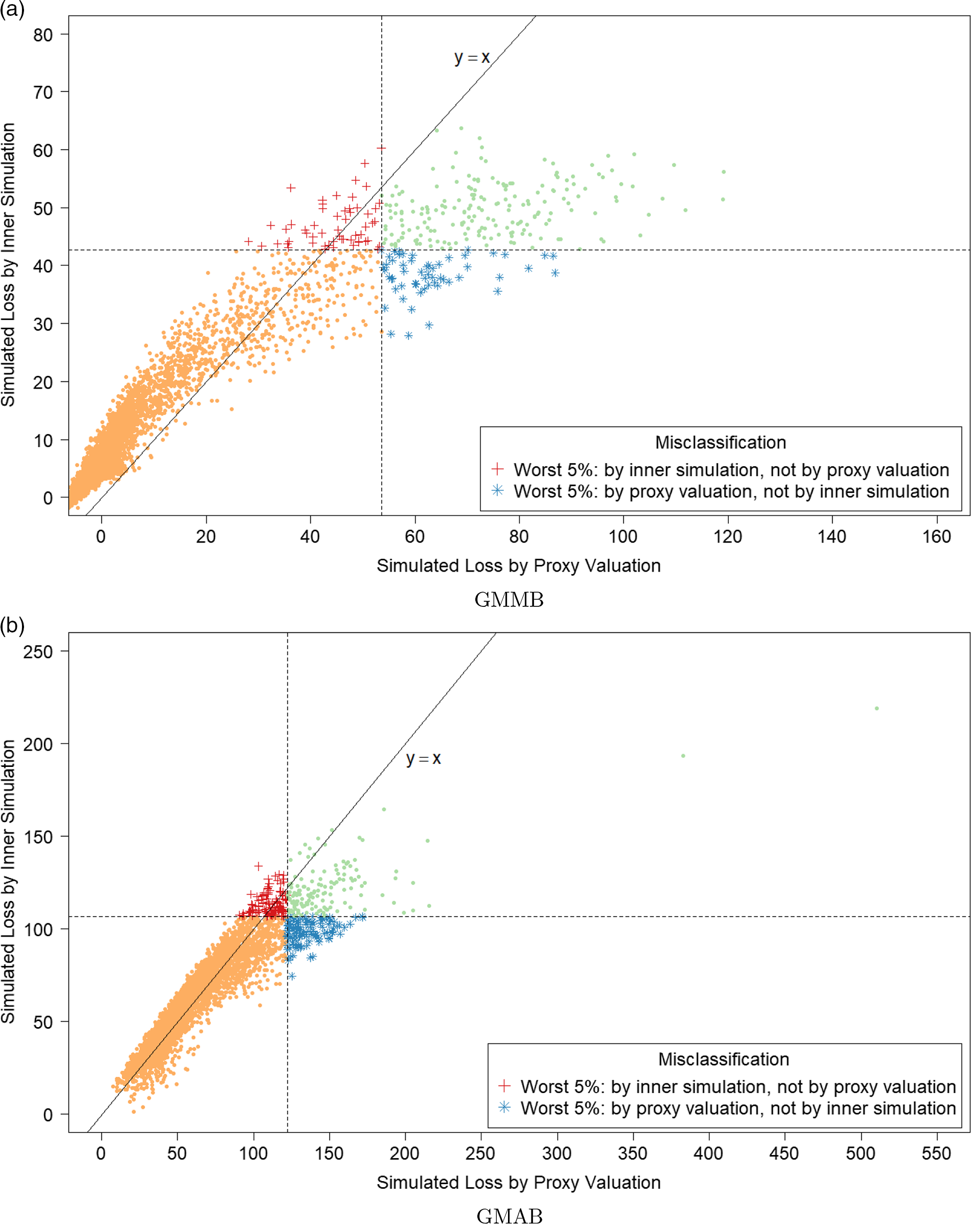
Figure 2. Simulated losses in 5,000 outer scenarios, by proxy valuation (x axis) and by inner simulation (y axis). Region above the horizontal line indicates the worst 5
 $\%$
loss by inner simulation. Region to the right of the vertical line indicates the worst 5
$\%$
loss by inner simulation. Region to the right of the vertical line indicates the worst 5
 $\%$
loss by proxy valuations.
$\%$
loss by proxy valuations.
We assume that we are interested in the 95
 $\%$
CTE, which involves the largest 250 losses from the 5,000 scenarios. The “+”’s in Figure 2 represent
$\%$
CTE, which involves the largest 250 losses from the 5,000 scenarios. The “+”’s in Figure 2 represent
 $\mathcal{T}_{250}\setminus\mathcal{T}^P_{250}$
, that is, the losses that are ranked in the top 5
$\mathcal{T}_{250}\setminus\mathcal{T}^P_{250}$
, that is, the losses that are ranked in the top 5
 $\%$
of the
$\%$
of the
 $L_i$
but are not in the top 5
$L_i$
but are not in the top 5
 $\%$
of the proxy loss estimates. The “
$\%$
of the proxy loss estimates. The “
 $*$
”’s represent
$*$
”’s represent
 $\mathcal{T}^P_{250}\setminus\mathcal{T}_{250}$
. Losses that lie on the right of the vertical line correspond to the worst 5
$\mathcal{T}^P_{250}\setminus\mathcal{T}_{250}$
. Losses that lie on the right of the vertical line correspond to the worst 5
 $\%$
proxy losses, while losses that lie above the horizontal line correspond to the worst 5
$\%$
proxy losses, while losses that lie above the horizontal line correspond to the worst 5
 $\%$
true losses.
$\%$
true losses.
In Figure 3, we show the quantile of the simulated losses presented in Figure 2. It suggests that the ranking of losses from inner simulation are reasonably well correlated to the ranking of losses from the proxy model.
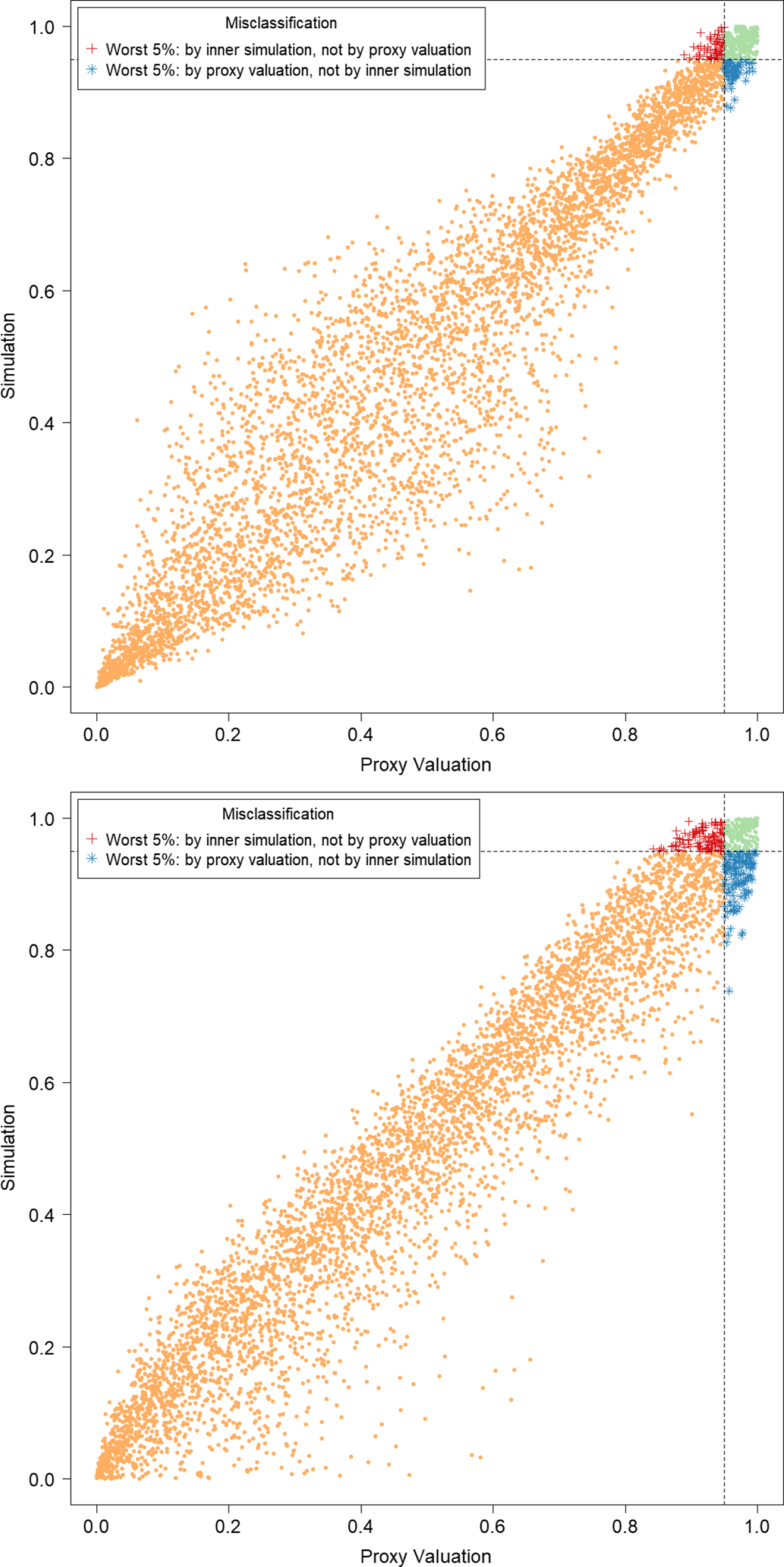
Figure 3. P–P plots of the simulated loss cumulative distribution functions in 5,000 outer scenarios, by proxy valuation (x axis) and by inner simulation (y axis); GMMB (top figure) and GMAB (bottom figure). The vertical and horizontal line represent the respective 95
 $\%$
quantile on the x and y axis.
$\%$
quantile on the x and y axis.
We note from Figures 2 and 3 that although the proxy model produces similar ranking of losses to the “true” losses, the actual values of the losses produced by the proxy model are very different to the accurate inner simulation model losses; the points in Figure 2 deviate significantly from the
 $y=x$
line in each plot. This means that we cannot simply use the proxy estimates of loss in the risk measure – we must proceed to the inner simulation step of the algorithm.
$y=x$
line in each plot. This means that we cannot simply use the proxy estimates of loss in the risk measure – we must proceed to the inner simulation step of the algorithm.
In addition, Figure 4 illustrates the final empirical copula used in applying the DIANS procedure to the 5,000 scenarios presented in Figure 2. The empirical copula suggests the proxy and inner simulation losses within the proxy tail scenarios set
 $\mathcal{T}^P_{\widetilde{m}}$
are also fairly well correlated, with the correlation in the empirical copula of the GMMB being stronger than that of GMAB. This has an impact on the number of proxy tail scenarios identified by the DIANS algorithm for the two different types of contracts, as we will see in section 4.4.
$\mathcal{T}^P_{\widetilde{m}}$
are also fairly well correlated, with the correlation in the empirical copula of the GMMB being stronger than that of GMAB. This has an impact on the number of proxy tail scenarios identified by the DIANS algorithm for the two different types of contracts, as we will see in section 4.4.
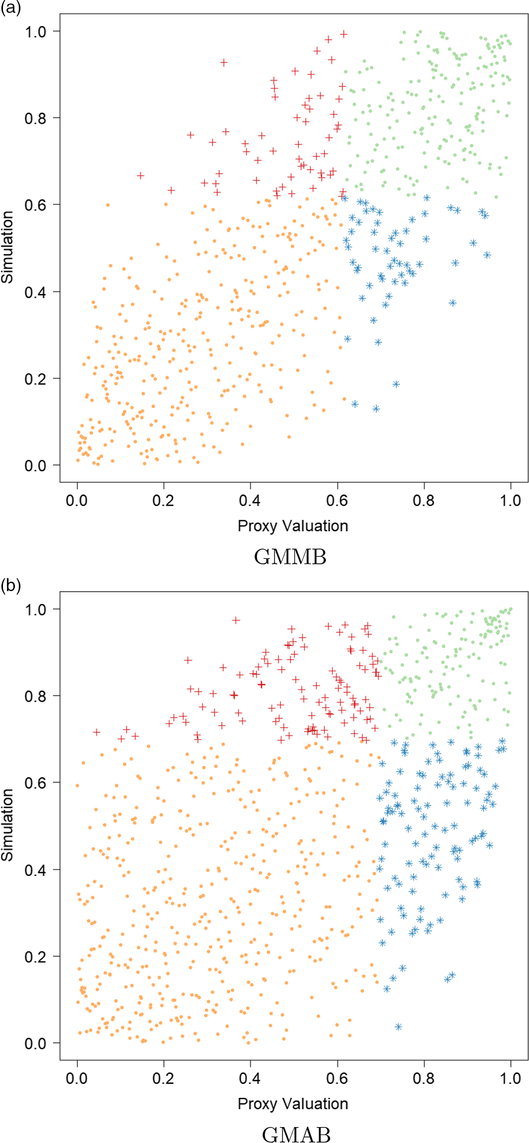
Figure 4. Empirical copula of simulated losses within the proxy tail scenarios set
 $\mathcal{T}^P_{\widetilde{m}}$
. The same legends as in Figure 2 are used.
$\mathcal{T}^P_{\widetilde{m}}$
. The same legends as in Figure 2 are used.
4.3 Identifying
 $\mathcal{T}^P_{\widetilde{m}}$

We explore the variables
 $m^*$
and
$m^*$
and
 $\widetilde{m}$
, where
$\widetilde{m}$
, where
 $\mathcal{T}^P_{m^*}$
is the smallest set of proxy tail scenarios containing
$\mathcal{T}^P_{m^*}$
is the smallest set of proxy tail scenarios containing
 $\mathcal{T}_{250}$
, and
$\mathcal{T}_{250}$
, and
 $\widetilde{m}$
is the number of proxy tail scenarios identified by the DIANS algorithm.
$\widetilde{m}$
is the number of proxy tail scenarios identified by the DIANS algorithm.
To do this, we run 20 repetitions of the DIANS algorithm, each using the same set of
 $M=5,000$
scenarios as used in the full uniform nested simulation, and each with the following input parameters:
$M=5,000$
scenarios as used in the full uniform nested simulation, and each with the following input parameters:
 \begin{align*}&\qquad \Gamma=5,000\times 200=10^6, \; N_0=1,000 , \; m_0=400, \; m^{\max}=5,000, \; d=150\end{align*}
Note that we have set
 $m^{\max}=M$
, which means that we have allowed the algorithm to continue to find an unconstrained value of
$m^{\max}=M$
, which means that we have allowed the algorithm to continue to find an unconstrained value of
 $\widetilde{m}$
. In practice,
$\widetilde{m}$
. In practice,
 $m^{\max}$
is a design variable that the user of the DIANS procedure would choose, based on the minimum acceptable number of inner simulations.
$m^{\max}$
is a design variable that the user of the DIANS procedure would choose, based on the minimum acceptable number of inner simulations.
From the full-scale uniform nested simulation, we know that the minimum number of proxy tail scenarios required to capture all the true tail scenarios is
 $m^*=\min\{m\,:\, \mathcal{T}_{250} \subset \mathcal{T}^P_m\} = 557$
.
$m^*=\min\{m\,:\, \mathcal{T}_{250} \subset \mathcal{T}^P_m\} = 557$
.
From the DIANS algorithm, for each repetition we record
 $ \widetilde{m}$
, which is the final number of scenarios in the proxy tail scenario set.
$ \widetilde{m}$
, which is the final number of scenarios in the proxy tail scenario set.
The results are illustrated in Figure 5. Each column represents a separate repetition of the DIANS valuation. In each column, the triangle represents
 $\widetilde{m}$
, which is the number of scenarios included in the tail scenario set using DIANS. The dots (which are the same in each column) represent the quantities
$\widetilde{m}$
, which is the number of scenarios included in the tail scenario set using DIANS. The dots (which are the same in each column) represent the quantities
 $M-R_{j\,:\,M}$
, for
$M-R_{j\,:\,M}$
, for
 $M=5,000$
, and
$M=5,000$
, and
 $j=4,751, 4,752, \ldots, 5,000$
. Here,
$j=4,751, 4,752, \ldots, 5,000$
. Here,
 $R_{j,M}$
is the concomitant rank of the jth true tail losses, so
$R_{j,M}$
is the concomitant rank of the jth true tail losses, so
 $M-R_{j\,:\,M}$
indicates the number of proxy tail scenarios required to capture the top
$M-R_{j\,:\,M}$
indicates the number of proxy tail scenarios required to capture the top
 $M-j$
true tail scenarios. The maximum value of
$M-j$
true tail scenarios. The maximum value of
 $M-R_{j\,:\,M}$
(i.e. the top dot in each column) is
$M-R_{j\,:\,M}$
(i.e. the top dot in each column) is
 $m^*$
, which is the number of proxy tail scenarios required to capture the scenarios generating the top 5
$m^*$
, which is the number of proxy tail scenarios required to capture the scenarios generating the top 5
 $\%$
of true losses.
$\%$
of true losses.
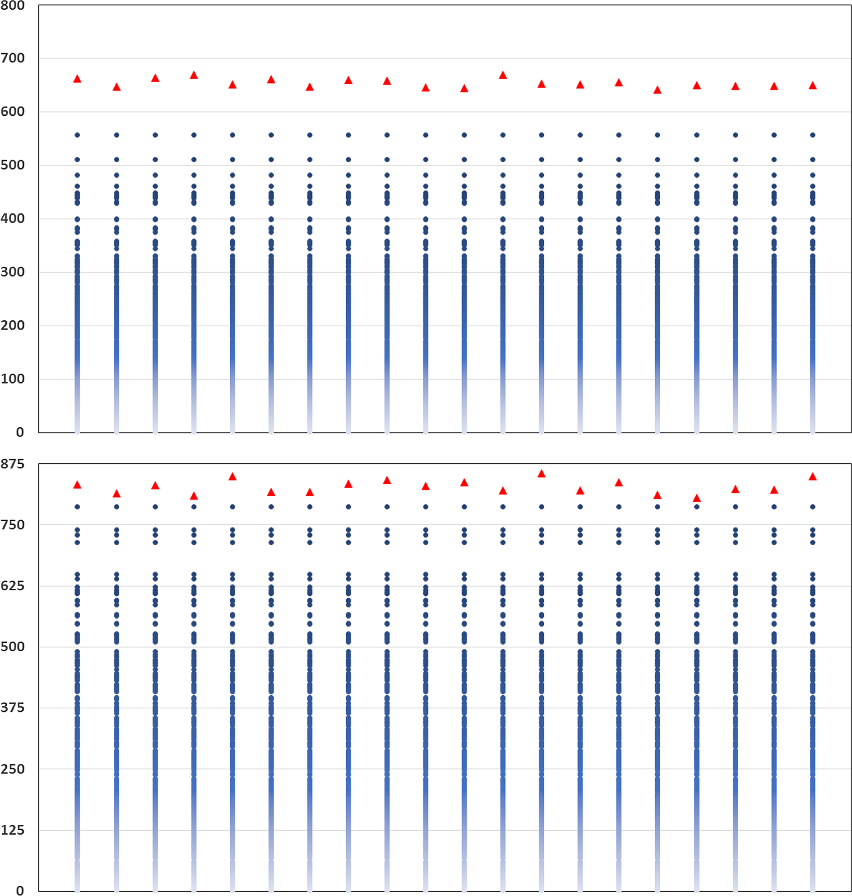
Figure 5. Actual inverse rank of concomitant of true tail losses and
 $\widetilde{m}$
(threshold generated by DIANS), for 20 repeated experiments described in section 4.3; GMMB (top) and GMAB (bottom).
$\widetilde{m}$
(threshold generated by DIANS), for 20 repeated experiments described in section 4.3; GMMB (top) and GMAB (bottom).
We see from the figure that
 $\widetilde{m}$
remains relatively stable across the experiments. We also see that for both the GMMB and the GMAB, in each of the 20 experiments, the threshold generated by the DIANS algorithm (the triangle) lies above the maximum required to capture all the true tail scenarios (represented by the uppermost dot), meaning that the algorithm generated a proxy tail set that included all the true tail scenarios. On the one hand, this is encouraging – the algorithm, here, does a good job of capturing all the true tail scenarios. On the other hand, in the GMMB case, the number of proxy tail scenarios selected is significantly greater than the number required to capture the true tail scenarios, signalling that we might be wasting computational effort. There is a trade-off here, between ensuring that the true tail scenarios are all captured, and ensuring that the inner simulation budget is sufficiently concentrated to give reliable results. The balance between these competing objectives can be adjusted by increasing or decreasing the confidence level used for the bound in Algorithm 2.
$\widetilde{m}$
remains relatively stable across the experiments. We also see that for both the GMMB and the GMAB, in each of the 20 experiments, the threshold generated by the DIANS algorithm (the triangle) lies above the maximum required to capture all the true tail scenarios (represented by the uppermost dot), meaning that the algorithm generated a proxy tail set that included all the true tail scenarios. On the one hand, this is encouraging – the algorithm, here, does a good job of capturing all the true tail scenarios. On the other hand, in the GMMB case, the number of proxy tail scenarios selected is significantly greater than the number required to capture the true tail scenarios, signalling that we might be wasting computational effort. There is a trade-off here, between ensuring that the true tail scenarios are all captured, and ensuring that the inner simulation budget is sufficiently concentrated to give reliable results. The balance between these competing objectives can be adjusted by increasing or decreasing the confidence level used for the bound in Algorithm 2.
4.4 CTE estimation
In this section, we compare the estimated 95
 $\%$
CTEs of the losses for both the GMMB and the GMAB described in section 4.1. We fix the inner simulation budget and apply the following estimation methods:
$\%$
CTEs of the losses for both the GMMB and the GMAB described in section 4.1. We fix the inner simulation budget and apply the following estimation methods:
-
(a) DIANS, as described in Algorithm 2, parameters as in the previous section.
-
(b) Fixed (non-dynamic) importance allocation nested simulation (Dang et al., Reference Dang, Feng and Hardy2020) with
-
(b1)
$m = 0.15 \times M=750$
. -
(b2)
$m = 0.10 \times M=500$
. -
(b3)
$m = 0.05 \times M=250$
. -
(c) Standard nested simulation with equal number of inner simulation.


Each experiment is repeated 100 times. The outer scenarios used for each repetition of each experiment are the same, so the differences between the results arise solely from tail scenario selection, and sampling variability at the inner simulation stage. The scenarios are also the same as those used for the large-scale nested simulations illustrated in Figure 2, which were used to calculate the accurate CTE estimate used as the basis for the root mean square error (RMSE) values below.
The inner simulation budget is fixed at
 $\Gamma=10^6$
. Using importance allocated nested simulation, with a fixed number of scenarios, m say, in the proxy tail scenario set, means that each scenario in the tail scenario set would be allocated
$\Gamma=10^6$
. Using importance allocated nested simulation, with a fixed number of scenarios, m say, in the proxy tail scenario set, means that each scenario in the tail scenario set would be allocated
 $10^6/m$
inner simulations, at each time step of the scenario.
$10^6/m$
inner simulations, at each time step of the scenario.
The DIANS approach uses the same inner simulation budget, but with a dynamic search algorithm to set the size of the proxy tail set. The additional run time created by the dynamic algorithm is negligible, so the different methods can be viewed as essentially equal in terms of the computational cost.
Table 1. Results from 100 repetitions of fixed and dynamic IANS process, and standard nested simulation, GMMB example, with standard errors. All values are based on a single outer scenario set.
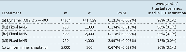
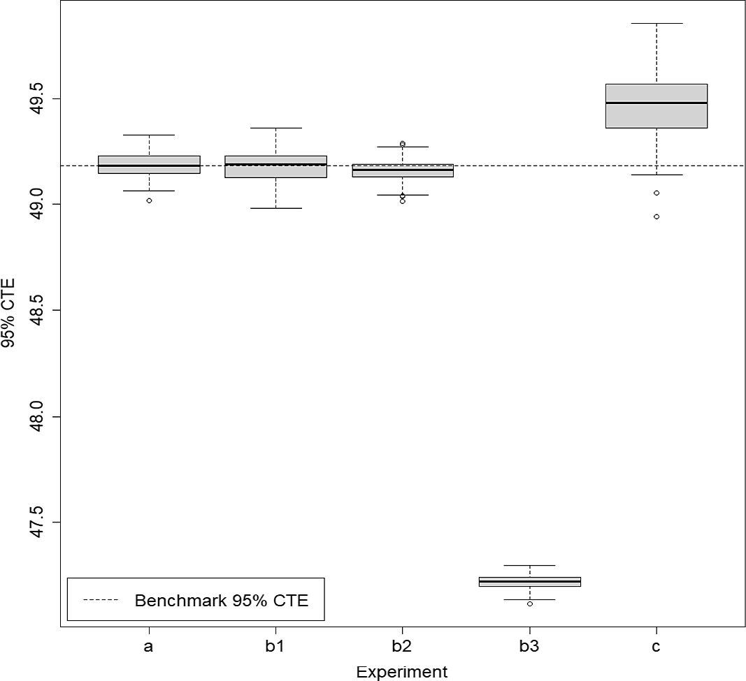
Figure 6. Box and whisker plot of results from 100 repetitions of fixed and dynamic IANS process and standard nested simulation, GMMB example.
The results for the GMMB experiments are summarised in Table 1 and are illustrated in the box and whisker plot in Figure 6. The results for the GMAB experiments are summarised in Table 2 and are illustrated in the box and whisker plot in Figure 7. In the tables, the RMSE is the root mean square error, expressed as a percentage of the accurate CTE value.
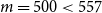
Table 2. Results from 100 repetitions of fixed and dynamic IANS process, and standard nested simulation, GMAB example, standard errors in brackets.
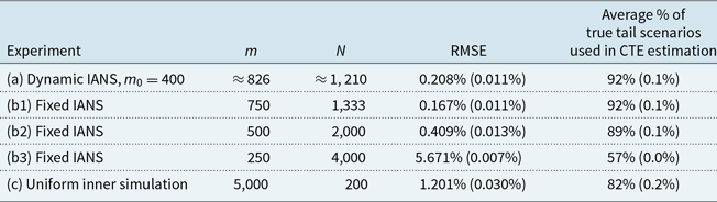
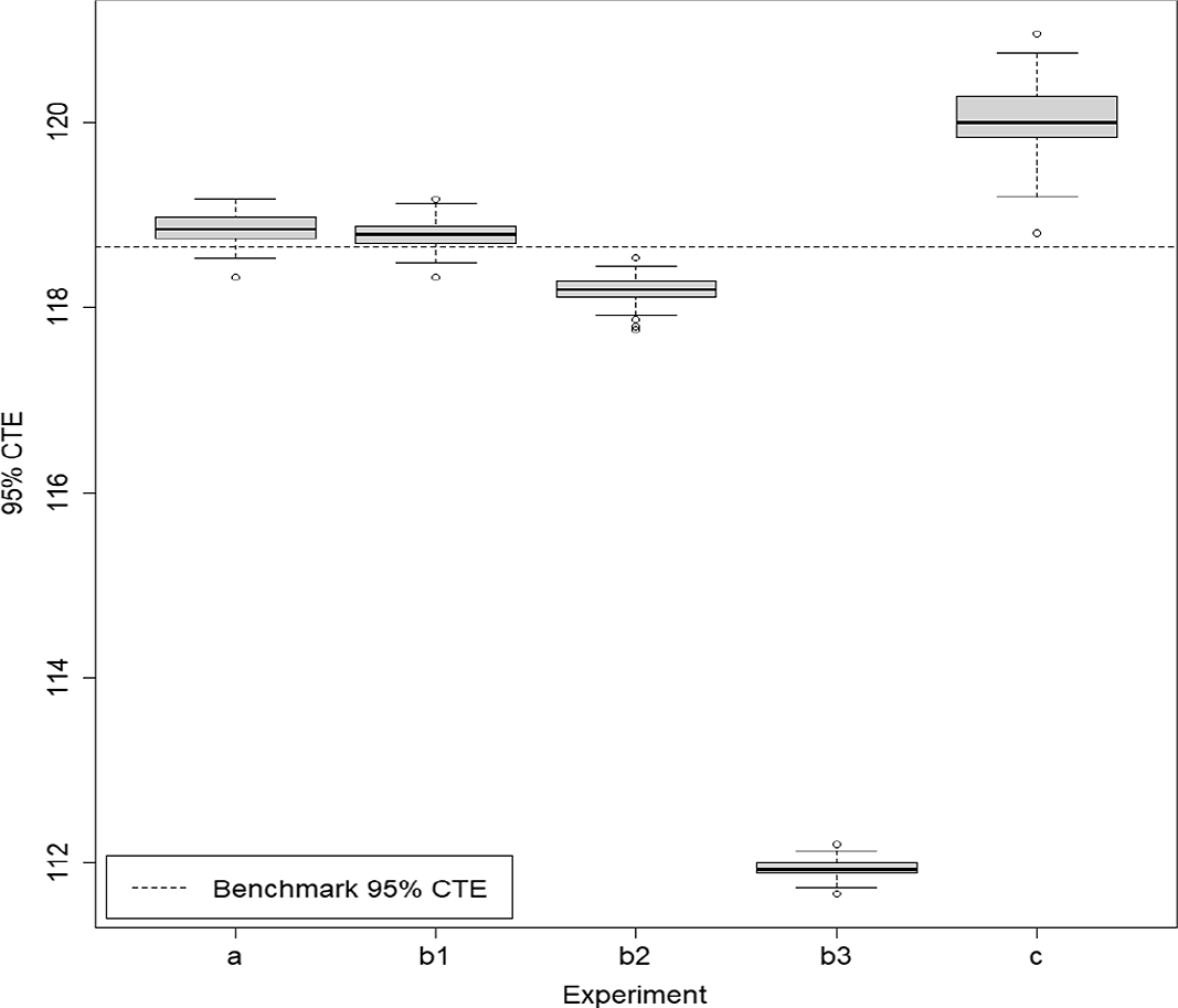
Figure 7. Box and whisker plot of results from 100 repetitions of fixed and dynamic IANS process and standard nested simulation, GMAB example.
In the final column of Table 1, we show the percentage of true tail scenarios used in the 95
 $\%$
CTE estimation of the GMMB experiments. In experiments (a) and (b1), although
$\%$
CTE estimation of the GMMB experiments. In experiments (a) and (b1), although
 $\mathcal{T}_{\widetilde{m}}$
captured all the true tail scenarios, the ranking of the tail scenarios in each case is not identical to the benchmark run due to inner simulation noise. As a result, only 96
$\mathcal{T}_{\widetilde{m}}$
captured all the true tail scenarios, the ranking of the tail scenarios in each case is not identical to the benchmark run due to inner simulation noise. As a result, only 96
 $\%$
of the true tail scenarios were used in the actual CTE calculation. We note from Figure 2 that, close to the threshold of the top 5
$\%$
of the true tail scenarios were used in the actual CTE calculation. We note from Figure 2 that, close to the threshold of the top 5
 $\%$
of true losses, the values of the losses immediately above the threshold are very close to the losses immediately below the threshold, so a small amount of replacement, in this example, makes little difference to the CTE estimation.
$\%$
of true losses, the values of the losses immediately above the threshold are very close to the losses immediately below the threshold, so a small amount of replacement, in this example, makes little difference to the CTE estimation.
In this example, the RMSE results suggest that the dynamic IANS procedure achieves significantly higher accuracy than IANS with fixed
 $m=250$
, achieves very similar results compared with IANS, with fixed
$m=250$
, achieves very similar results compared with IANS, with fixed
 $m=750$
or
$m=750$
or
 $m=500$
, and significantly outperforms the uniform inner simulation method.
$m=500$
, and significantly outperforms the uniform inner simulation method.
The RMSEs in methods (a), (b1) and (b2) are similar because the minimum number of proxy tail scenarios required to capture the full set of true tail scenarios is
 $m^*=557$
(for this set of
$m^*=557$
(for this set of
 $\mathbf{\omega}$
). Thus, any importance allocation method with
$\mathbf{\omega}$
). Thus, any importance allocation method with
 $m > 557$
would capture all the true tail scenarios, and that includes the DIANS case (m exceeded 557 in each of the 100 repetitions) and the fixed IANS case with
$m > 557$
would capture all the true tail scenarios, and that includes the DIANS case (m exceeded 557 in each of the 100 repetitions) and the fixed IANS case with
 $m=750$
. For the fixed IANS case with
$m=750$
. For the fixed IANS case with
 $m=500<557$
, some true tail scenarios are omitted from the inner simulation stage; from the top plot in Figure 5, by looking at the number of dots lying above the
$m=500<557$
, some true tail scenarios are omitted from the inner simulation stage; from the top plot in Figure 5, by looking at the number of dots lying above the
 $y=500$
line, we see that using 500 proxy tail scenarios will miss just 2 true tail scenarios. Even though the true tail scenarios are all, or almost all captured in experiments (a), (b1) and (b2), the losses for the tail scenarios are estimated with different numbers of inner simulations in each of the three experiments. The difference in RMSE between experiments (a) and (b1) is driven entirely by the difference in the number of inner simulations deployed to each scenario in
$y=500$
line, we see that using 500 proxy tail scenarios will miss just 2 true tail scenarios. Even though the true tail scenarios are all, or almost all captured in experiments (a), (b1) and (b2), the losses for the tail scenarios are estimated with different numbers of inner simulations in each of the three experiments. The difference in RMSE between experiments (a) and (b1) is driven entirely by the difference in the number of inner simulations deployed to each scenario in
 $\mathcal{T}_{m}$
; both methods capture all the true tail scenarios, but the DIANS method does so with less redundancy, and therefore more accuracy in the loss estimation. This is illustrated in Figure 6, which shows that both experiments appear to generate unbiased estimators, but the variance of (b1) is a little greater than the variance of (a). Experiment (b2) misses two true tail scenarios, but achieves more accurate results for those that it does capture. Because it misses some true tail scenarios, the CTE estimate is biased low (as we can see in Figure 6). However, in this case, the bias is compensated by the low variance in the RMSE calculation.
$\mathcal{T}_{m}$
; both methods capture all the true tail scenarios, but the DIANS method does so with less redundancy, and therefore more accuracy in the loss estimation. This is illustrated in Figure 6, which shows that both experiments appear to generate unbiased estimators, but the variance of (b1) is a little greater than the variance of (a). Experiment (b2) misses two true tail scenarios, but achieves more accurate results for those that it does capture. Because it misses some true tail scenarios, the CTE estimate is biased low (as we can see in Figure 6). However, in this case, the bias is compensated by the low variance in the RMSE calculation.
In contrast, the RMSE under experiment (b3) is close to 30 times that of the DIANS result. Experiment (b3) uses a fixed m of only 250, allowing no cushion for losses that are in the top 5
 $\%$
under the accurate calculation, but are below the top 5
$\%$
under the accurate calculation, but are below the top 5
 $\%$
by the proxy calculation. The evaluation of loss for each scenario in the proxy tail set will be more accurate, using 4,000 inner simulations, but many true tail scenarios are missed in this experiment. The missed tail scenarios are replaced with others that are lesser ranked, based on the initial simulation values, so the CTE estimate is, again, biased low – much more significantly than in (b2). Note that, comparing the result from method (b3) with the uniform nested simulation result, in method (c), we see that if the importance allocation method misses too many true tail scenarios the result is actually worse than using a uniform allocation of inner simulation under the same budget. This underscores the usefulness of using the dynamic IANS procedure to ensure sufficient tail scenario coverage, rather than a fixed IANS method. In practice, we do not know the value of
$\%$
by the proxy calculation. The evaluation of loss for each scenario in the proxy tail set will be more accurate, using 4,000 inner simulations, but many true tail scenarios are missed in this experiment. The missed tail scenarios are replaced with others that are lesser ranked, based on the initial simulation values, so the CTE estimate is, again, biased low – much more significantly than in (b2). Note that, comparing the result from method (b3) with the uniform nested simulation result, in method (c), we see that if the importance allocation method misses too many true tail scenarios the result is actually worse than using a uniform allocation of inner simulation under the same budget. This underscores the usefulness of using the dynamic IANS procedure to ensure sufficient tail scenario coverage, rather than a fixed IANS method. In practice, we do not know the value of
 $m^*$
; the advantage of the dynamic IANS procedure is that we eliminate the subjectivity involved in selecting a fixed m.
$m^*$
; the advantage of the dynamic IANS procedure is that we eliminate the subjectivity involved in selecting a fixed m.
Note that the positive bias indicated in the uniform nested simulation approach (experiment (c)) results from evaluating discrete hedging errors for out-of-the-money options with a small number of simulations (Boyle & Emanuel, Reference Boyle and Emanuel1980).
In the GMAB case, the greater volatility in estimated losses for each scenario means that a larger number of additional proxy tail scenarios are required to capture all 250 true tail scenarios. GMABs involve very significant gamma risk (Hardy, Reference Hardy2003), particularly at the renewal dates, when the delta of the option can decline sharply from positive to negative. There is, therefore, significantly more hedging error from a delta hedge of a GMAB than of the GMMB. For this set of scenarios, the number of proxy tail scenarios required to capture all 250 true tail scenarios is
 $m^*=787$
. The DIANS method captures all these scenarios, with an average m of 826, but with only (on average) 1,210 inner simulations allocated to the valuation for each step in each scenario; this number is relatively small, leading to a small positive bias in the estimation. The fixed IANS method with
$m^*=787$
. The DIANS method captures all these scenarios, with an average m of 826, but with only (on average) 1,210 inner simulations allocated to the valuation for each step in each scenario; this number is relatively small, leading to a small positive bias in the estimation. The fixed IANS method with
 $m=750$
captures all but one of the true tail scenarios and has a slightly higher inner simulation budget than the DIANS method, with the result that the RMSE is slightly better than the DIANS method. Experiments (b2) and (b3) both have values of m that are too small, missing a significant number of true tail scenarios, creating an estimate that is biased low, with much larger RMSEs. The result for the uniform nested simulation method is similar to the GMMB case.
$m=750$
captures all but one of the true tail scenarios and has a slightly higher inner simulation budget than the DIANS method, with the result that the RMSE is slightly better than the DIANS method. Experiments (b2) and (b3) both have values of m that are too small, missing a significant number of true tail scenarios, creating an estimate that is biased low, with much larger RMSEs. The result for the uniform nested simulation method is similar to the GMMB case.
4.5 VaR estimation
In this section, we repeat the DIANS (experiment (a)) and standard nested simulation (experiment (c)) in section 4.4, but for a 99
 $\%$
VaR estimation. The purpose of these experiments is to demonstrate the gain in computation efficiency by applying the DIANS procedure in a quantile risk measure estimation further into the tail region of the loss distribution.
$\%$
VaR estimation. The purpose of these experiments is to demonstrate the gain in computation efficiency by applying the DIANS procedure in a quantile risk measure estimation further into the tail region of the loss distribution.
We apply the same experiment setting and used the same sets of outer scenarios for GMMB and GMAB, respectively, as in section 4.4. The DIANS experiment was conducted using Algorithm 2 with
 $\alpha = 99\%$
and the VaR estimator in equation (9).
$\alpha = 99\%$
and the VaR estimator in equation (9).
The parameters and results of the experiments are summarised in Table 3. The results are also illustrated in the box and whisker plots in Figure 8.
Table 3. 99
 $\%$
VaR results from 100 repetitions of dynamic IANS process and standard nested simulation. Standard error of the results indicated in bracket. All values are based on a single outer scenario set,
$\%$
VaR results from 100 repetitions of dynamic IANS process and standard nested simulation. Standard error of the results indicated in bracket. All values are based on a single outer scenario set,
 $\mathbf{\omega}$
.
$\mathbf{\omega}$
.
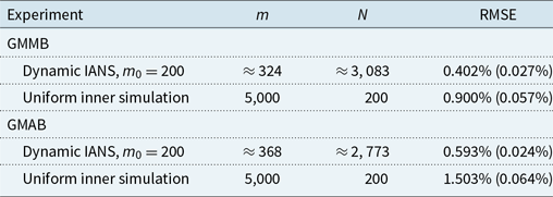
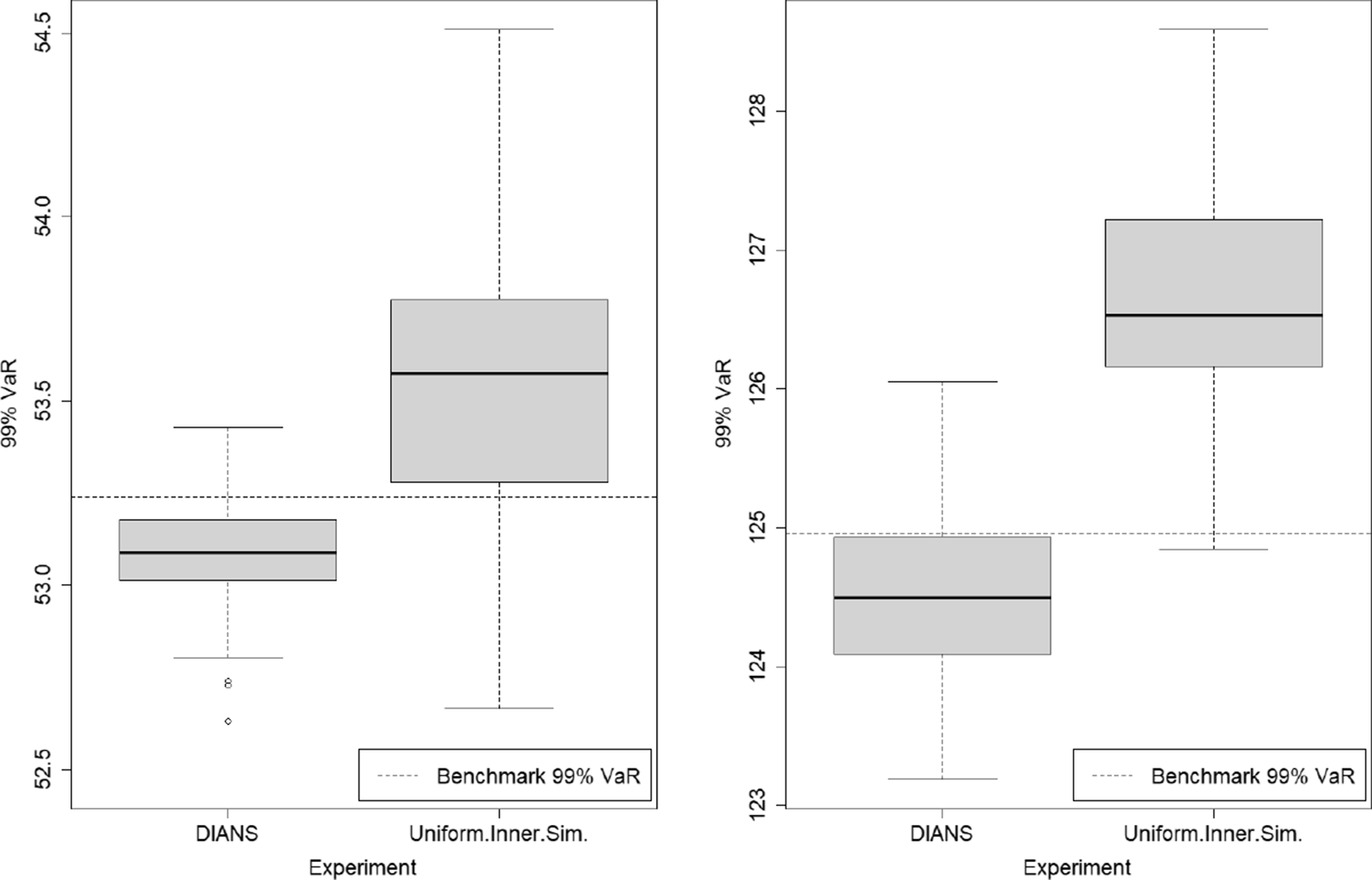
Figure 8. Box and whisker plot of 99
 $\%$
VaR results from 100 repetitions of fixed and dynamic IANS process, and standard nested simulation, GMMB (left) and GMAB (right) example.
$\%$
VaR results from 100 repetitions of fixed and dynamic IANS process, and standard nested simulation, GMMB (left) and GMAB (right) example.
Given the same computation budget, the DIANS procedure achieves an RMSE of less than 1/2 of the standard nested simulation method. The improvement is less significant than that observed in the CTE estimation. There are two main reasons for this. The first is that in nested simulations, as the number of inner simulation increases, the bias of the estimated CTE reduces faster than bias of the estimated VaR; see the convergence results derived in Gordy & Juneja (Reference Gordy and Juneja2010). The second reason is that there is more variance in the VaR estimate than the CTE estimate. The CTE is estimated by taking the average of all relevant tail scenario loss, which smooths out some variations in losses of individual tail scenarios. In contrast, the VaR is only a weighted average of losses in two individual tail scenarios.
We also observe that the DIANS procedure results in a negative bias in the VaR estimate, whereas the standard nested simulation results in a positive bias. In the standard nested simulation, due to inner simulation noise some non-tail scenarios are misclassified as tail scenarios. Moreover, as we are interested in scenarios with the highest losses, scenarios with positive biases are more likely to be (mis)classified as tail scenarios and carried to the tail risk estimate (VaR or CTE). As Gordy & Juneja (Reference Gordy and Juneja2010) point out, this positive bias in standard nested simulation diminishes as computational budget increases.
The negative bias in the DIANS procedure is caused by possible misclassification of non-tail scenarios in the proxy tail scenario set, similar to our observation in experiment (b3) in the CTE experiments (see Figures 6 and 7). The misclassified non-tail scenarios inherently have lower loss estimates which is estimated more accurately in the DIANS procedure due to concentration in the computational budget. As a result, a negative bias in the tail risk measure occurs when misclassification of non-tail scenarios happens.
With a higher computational budget, the DIANS procedure would identify the tail scenarios more accurately by deploying more inner simulations in the pilot runs. This would lead a more accurate estimate of ranking of scenarios and eventually eliminate the negative bias in VaR estimation.
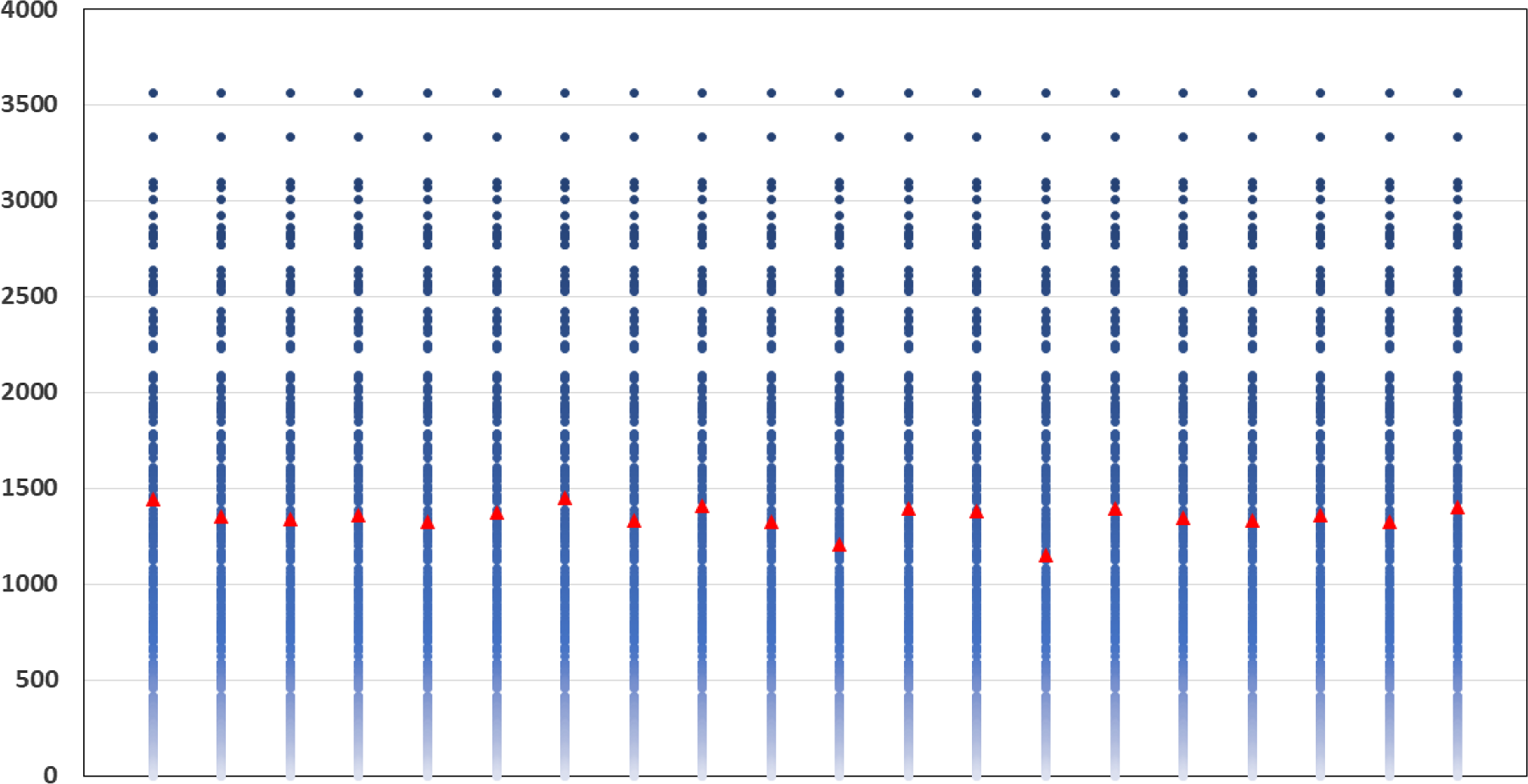
Figure 9. Actual inverse rank of concomitant of true tail scenarios and and
 $\widetilde{m}$
(threshold generated by DIANS), in 20 repeated experiments in section 4.6 (sensitivity test).
$\widetilde{m}$
(threshold generated by DIANS), in 20 repeated experiments in section 4.6 (sensitivity test).
4.6 Identifying a bad proxy
With all methods based on proxy modelling, there is a risk that, over time, the relationship between the true loss and the proxy loss can deteriorate; the simplifications used in the proxy model may drift too far from the real-world experience, or the proxy model parameters may need to be updated. An advantage of the DIANS approach is that the suitability of the proxy model can be assessed directly using the DIANS output, without the need for additional backtesting.
To illustrate, we repeat the experiment from section 4.3, but with very different parameters for the fund returns, specified in Appendix B.2. These parameters generate prolonged periods of very poor mean returns and very high volatility.
The results are shown in Figure 9. As in Figure 5, each column represents a repetition of the DIANS procedure under shocked parameters. The highest dot marks
 $m^*$
, the minimum number of proxy scenarios required to capture the true 5
$m^*$
, the minimum number of proxy scenarios required to capture the true 5
 $\%$
tail scenarios, and the triangle represents the cut-off identified by the DIANS algorithm, but without the constraint in Line 14 of Algorithm 2, that
$\%$
tail scenarios, and the triangle represents the cut-off identified by the DIANS algorithm, but without the constraint in Line 14 of Algorithm 2, that
 $m_k \leq m^{\max}$
. In fact, in all cases, the algorithm would be stopped as
$m_k \leq m^{\max}$
. In fact, in all cases, the algorithm would be stopped as
 $m_k$
exceeds the maximum of 1,000 scenarios. A small amount of investigation in this case indicates that the constant lapse assumption used in the proxy is not sufficiently accurate when the fund returns are consistently poor for long periods, as is the case under the new parameters. A small change to the lapse assumption restores the proxy model as an adequate signal for the tail scenarios.
$m_k$
exceeds the maximum of 1,000 scenarios. A small amount of investigation in this case indicates that the constant lapse assumption used in the proxy is not sufficiently accurate when the fund returns are consistently poor for long periods, as is the case under the new parameters. A small change to the lapse assumption restores the proxy model as an adequate signal for the tail scenarios.

Figure 10. Examples of empirical copulas for proxy tail scenario sets.
Checking how close
 $\widetilde{m}$
is to
$\widetilde{m}$
is to
 $m^{\max}$
is only one way that the DIANS procedure signals an inadequate proxy. Other indicators include the following.
$m^{\max}$
is only one way that the DIANS procedure signals an inadequate proxy. Other indicators include the following.
The Spearman’s rank correlation can be calculated for the
$\widetilde{m}$
proxy losses and simulated losses in the proxy tail scenario set. A strong proxy will have a rank correlation, greater than, say, 0.75. An adequate proxy will have a rank correlation of at least around 0.6. Lower correlations indicate that the proxy needs to be updated.The plots of
$(U^P_j, \widehat{U}_j)$
(which are
$p{-}p$
plots for the proxy and simulated losses), generated by successive iterations of
$m_k$
, can give a visual signal of the proxy model adequacy. If the proxy is working well, then the
$p{-}p$
plots will show strong clustering around the
$y=x$
line through successive iterations. If there are a significant number of outliers, that could indicate that the proxy is systematically missing some of the true tail scenarios.


In Figure 10, we show examples of copulas generated by successful and unsuccessful proxies. In each case,
 $M=5,000$
and
$M=5,000$
and
 $m_0 = 400$
. Figure 10(a) shows the same copula in the GMMB experiment as in Figure 4(a). As discussed in section 4.2, the proxy is a good indicator of the ranking of the losses. The Spearman’s correlation coefficient was
$m_0 = 400$
. Figure 10(a) shows the same copula in the GMMB experiment as in Figure 4(a). As discussed in section 4.2, the proxy is a good indicator of the ranking of the losses. The Spearman’s correlation coefficient was
 $\rho^s=0.6$
on the first iteration of the algorithm, and
$\rho^s=0.6$
on the first iteration of the algorithm, and
 $\rho^s=0.8$
on the third and final iteration, and
$\rho^s=0.8$
on the third and final iteration, and
 $\widetilde{m}$
ended at 652 scenarios.
$\widetilde{m}$
ended at 652 scenarios.
Figure 10(b) shows the copula from the GMAB experiment. As mentioned earlier, this is a less accurate proxy than the GMMB case. The Spearman’s correlation coefficient was
 $\rho^s=0.4$
on the first iteration of the algorithm, and
$\rho^s=0.4$
on the first iteration of the algorithm, and
 $\rho^s=0.6$
on the third and final iteration, and
$\rho^s=0.6$
on the third and final iteration, and
 $\widetilde{m}$
ended at 823 scenarios.
$\widetilde{m}$
ended at 823 scenarios.
In Figure 10(c), the
 $p{-}p$
plot indicates that the proxy is not a good indicator of the ranking of the simulated losses. The Spearman’s correlation coefficient in this example was
$p{-}p$
plot indicates that the proxy is not a good indicator of the ranking of the simulated losses. The Spearman’s correlation coefficient in this example was
 $\rho^s=0.2$
on the first iteration of the algorithm, and
$\rho^s=0.2$
on the first iteration of the algorithm, and
 $\rho^s=0.3$
on the fourth and final iteration. The final
$\rho^s=0.3$
on the fourth and final iteration. The final
 $\widetilde{m}$
was close to 1,400 scenarios.
$\widetilde{m}$
was close to 1,400 scenarios.
In Figure 10(d), the copula indicates that the proxy is capturing some of the tail scenarios, but is also misclassifying some. This can happen, for example, for more complex payouts with two triggers, and where the proxy only captures one trigger. The Spearman’s correlation coefficient in this case was
 $\rho^s=0.55$
on the first iteration, and
$\rho^s=0.55$
on the first iteration, and
 $\rho^s=0.56$
on the seventh and final iteration. The final number of scenarios in
$\rho^s=0.56$
on the seventh and final iteration. The final number of scenarios in
 $\mathcal{T}^P_{\widetilde{m}}$
was just under 600, which would not indicate that the proxy was inadequate. The only signals here of an inadequate proxy are the Spearman’s rho and the
$\mathcal{T}^P_{\widetilde{m}}$
was just under 600, which would not indicate that the proxy was inadequate. The only signals here of an inadequate proxy are the Spearman’s rho and the
 $p{-}p$
plot.
$p{-}p$
plot.
5. Conclusion
In both insurance and finance, risk management of more sophisticated products, with longer horizons, and with more complex economic capital requirements, is creating computational complexity that challenges even the most powerful computing environments. The development of efficient, accurate and implementable computational tools is important and timely. The DIANS method provides a practical tool for nested simulation in insurance liability measurement and has potential for application to a wider range of problems, including, for example, assessing semi-static hedging strategies, estimating multi-period risk measures (Hardy & Wirch, Reference Hardy and Wirch2004; Devolder & Lebègue, Reference Devolder and Lebègue2017), and calculating Solvency II regulatory capital requirements (Bauer et al., Reference Bauer, Reuss and Singer2012). It is particularly useful for path-dependent problems, where the non-uniform allocation approaches of Gordy & Juneja (Reference Gordy and Juneja2010) and Broadie et al. (Reference Broadie, Du and Moallemi2011) are not directly applicable. Compared with full proxy model approaches, the DIANS offers more accurate calculation and also signals an inadequate or ineffective proxy. The extra calculation involved in the process of finding the appropriate size for the proxy tail scenario set is minor, compared with the computational cost of additional simulations.
The identification and implementation of a suitable proxy model is a large part of this methodology. For most VA guarantees with lump-sum benefits (i.e. excluding GMWBs and GMIBs) the Black–Scholes option pricing framework provides the obvious resource. Complex VA guarantees can be mapped to formulas or numerical approximations developed for exotic options; for example, the GMMB with resets is very similar to a “put-on-the-max,” or high water mark option, for which a valuation formula was provided in Goldman et al. (Reference Goldman, Sosin and Gatto1979).
Where no tractable Black–Scholes valuation approach is available, the proxy model is most likely to be generated intrinsically. This may involve a regular calibration exercise to construct empirical valuation functions based on key scenario variables. The PDE valuation method of Feng (Reference Feng2014) could be used to construct a proxy model, which can then be combined with targeted inner simulations. In Dang et al. (Reference Dang, Feng and Hardy2021), the proxy model is replaced with a pilot simulation using common set of inner simulations, with the inner simulation probabilities adjusted for each scenario using a likelihood ratio approach.
Acknowledgements
This project was supported by the Natural Sciences and Engineering Research Council of Canada (NSERC), funding reference numbers RGPIN-2018-03754 (Hardy) and RGPIN-2018-03755(Feng). Ou Dang is supported through the Society of Actuary’s Hickman Scholarship programme.
The authors wish to acknowledge the very helpful suggestions of an anonymous referee.
A. Proof of Proposition 3.1
For a general bivariate distribution of (U,V), from David et al. (Reference David, O’Connell and Yang1977), we have
 \begin{align}&E[R_{j\,:\,m}]= 1 + m \left(\int\limits_\infty^{-\infty} \left[\int\limits_\infty^{-\infty} \theta_1 f(v \vert u) dv\right] f_{U_{j-1\,:\,m-1}}(u)du + \int\limits_\infty^{-\infty} \left[\int\limits_\infty^{-\infty} \theta_3 f(v \vert u) dv\right] f_{U_{j\,:\,m-1}}(u)du\right)\end{align}
where
 \begin{align*}&\theta_1 = P[U < u, V < v], \quad \theta_2 = P[U < u, V > v],\quad \theta_3 = P[U > u, V < v], \quad \theta_4 = P[U > u, V > v]\end{align*}
If (U,V) has a bivariate uniform distribution, we have
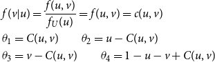 \begin{align*} & f(v \vert u) = \frac{f(u,v)}{f_U(u)} = f(u,v) = c(u,v)\\ &\theta_1 = C(u,v) \qquad \theta_2 = u - C(u,v)\\&\theta_3 = v - C(u,v) \qquad \theta_4 = 1-u - v + C(u,v)\end{align*}
where
C(u,v) is the copula function of
 $U = u$
and
$U = u$
and
 $V=v$
.
$V=v$
.
c(u,v) is the density function of C(U,V).
 $f_{U_{j\,:\,m}}(u)$
represents the density function of the jth order statistic among m U’s:
$f_{U_{j\,:\,m}}(u)$
represents the density function of the jth order statistic among m U’s:
 \begin{align*}&f_{U_{j\,:\,m}}(u) = \frac{m!}{(j-1)!(m-j)!} u^{j-1}(1-u)^{m-j}.\end{align*}
Therefore, in thiscase, equation (A.1) is equivalent to
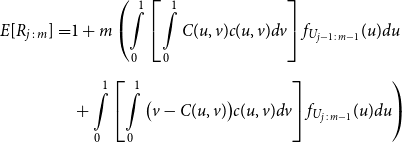 \begin{align}E[R_{j\,:\,m}] = & 1 + m \left(\int\limits_0^1 \left[\int\limits_0^1 C(u,v) c(u,v) dv\right]f_{U_{j-1\,:\,m-1}}(u)du \right.\nonumber\\[5pt]& \left.+ \int\limits_0^1 \left[\int\limits_0^1 \big(v - C(u,v)\big) c(u,v) dv\right] f_{U_{j\,:\,m-1}}(u)du\right) \end{align}
To derive the second moment of
 $R_{j\,:\,m}$
, we first derive the second moment of
$R_{j\,:\,m}$
, we first derive the second moment of
 $R_{j\,:\,m}$
for a general bivariate pair, (X,Y), that is, not specifically bivariate uniform distributed. We use the same factorial moment method as in O’Connell (Reference O’Connell1974).
$R_{j\,:\,m}$
for a general bivariate pair, (X,Y), that is, not specifically bivariate uniform distributed. We use the same factorial moment method as in O’Connell (Reference O’Connell1974).
First, we have
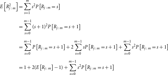 \begin{align}E\left[R_{j\,:\,m}^2\right] &= \sum_{s=1}^m s^2 P\left[R_{j\,:\,m} = s\right]\nonumber\\[5pt]&= \sum_{s=0}^{m-1} (s+1)^2 P\left[R_{j\,:\,m} = s+1\right]\nonumber\\[5pt]&= \sum_{s=0}^{m-1} P\left[R_{j\,:\,m} = s+1\right]+ 2\sum_{s=0}^{m-1} s P\left[R_{j\,:\,m} = s+1\right] + \sum_{s=0}^{m-1} s^2 P\left[R_{j\,:\,m} = s+1\right]\nonumber \\[5pt]&= 1+ 2(E\left[R_{j\,:\,m}\right]-1) + \sum_{s=0}^{m-1} s^2 P\left[R_{j\,:\,m} = s+1\right]\end{align}
More specifically,
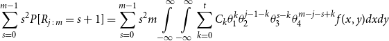 \begin{align}& \sum_{s=0}^{m-1} s^2 P[R_{j\,:\,m} = s+1]= \sum_{s=0}^{m-1} s^2 m \int\limits_{-\infty}^{\infty}\int\limits_{-\infty}^{\infty}\sum_{k=0}^t C_k \theta_1^k \theta_2^{j-1-k}\theta_3^{s-k}\theta_4^{m-j-s+k}f(x,y)dxdy \end{align}
where
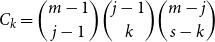 $ C_k = \displaystyle\binom{m-1}{j-1} \displaystyle\binom{j-1}{k} \displaystyle\binom{m-j}{s-k} $
Let
 $i=s-k$
, then
$i=s-k$
, then
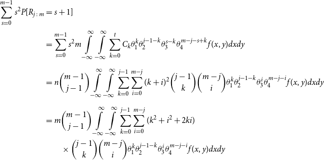 \begin{align}\sum_{s=0}^{m-1} s^2 P[R_{j\,:\,m} & = s+1]\nonumber\\[1pt]& = \sum_{s=0}^{m-1} s^2 m \int\limits_{-\infty}^{\infty}\int\limits_{-\infty}^{\infty}\sum_{k=0}^t C_k \theta_1^k \theta_2^{j-1-k}\theta_3^{s-k}\theta_4^{m-j-s+k}f(x,y)dxdy\nonumber\\[5pt]& = n\binom{m-1}{j-1} \int\limits_{-\infty}^{\infty}\int\limits_{-\infty}^{\infty} \sum_{k=0}^{j-1} \sum_{i=0}^{m-j} (k+i)^2 \binom{j-1}{k} \binom{m-j}{i} \theta_1^k \theta_2^{j-1-k}\theta_3^i\theta_4^{m-j-i}f(x,y)dxdy\nonumber\\[5pt]& = m\binom{m-1}{j-1} \int\limits_{-\infty}^{\infty}\int\limits_{-\infty}^{\infty} \sum_{k=0}^{j-1} \sum_{i=0}^{m-j} (k^2+i^2+ 2ki)\nonumber\\& \qquad \times \binom{j-1}{k} \binom{m-j}{i} \theta_1^k \theta_2^{j-1-k}\theta_3^i\theta_4^{m-j-i}f(x,y)dxdy\end{align}
Furthermore,
 \begin{align} & m\binom{m-1}{j-1}\int\limits_{-\infty}^{\infty}\int\limits_{-\infty}^{\infty} \sum_{k=0}^{j-1} \sum_{i=0}^{m-j} k^2 \binom{j-1}{k} \binom{m-j}{i} \theta_1^k \theta_2^{j-1-k}\theta_3^i\theta_4^{m-j-i}f(x,y)dxdy\nonumber\\[5pt]& = m\binom{m-1}{j-1}\int\limits_{-\infty}^{\infty}\int\limits_{-\infty}^{\infty} \sum_{k=0}^{j-1} \sum_{i=0}^{m-j} k(k-1) \binom{j-1}{k} \binom{m-j}{i} \theta_1^k \theta_2^{j-1-k}\theta_3^i\theta_4^{m-j-i}f(x,y)dxd \nonumber\end{align}
 \begin{align}& \quad + m\binom{m-1}{j-1}\int\limits_{-\infty}^{\infty}\int\limits_{-\infty}^{\infty} \sum_{k=0}^{j-1} \sum_{i=0}^{m-j} k \binom{j-1}{k} \binom{m-j}{i} \theta_1^k \theta_2^{j-1-k}\theta_3^i\theta_4^{m-j-i}f(x,y)dxdy\nonumber\\[5pt]& = m\binom{m-1}{j-1}\int\limits_{-\infty}^{\infty}\int\limits_{-\infty}^{\infty} \sum_{k=0}^{j-1} k(k-1) \binom{j-1}{k} \theta_1^k \theta_2^{j-1-k} \sum_{i=0}^{m-j}\binom{m-j}{i} \theta_3^i\theta_4^{m-j-i}f(x,y)dxdy\nonumber\\[5pt]& \quad + m\binom{m-1}{j-1}\int\limits_{-\infty}^{\infty}\int\limits_{-\infty}^{\infty} \sum_{k=0}^{j-1} k \binom{j-1}{k} \theta_1^k \theta_2^{j-1-k}\sum_{i=0}^{m-j}\binom{m-j}{i} \theta_3^i\theta_4^{m-j-i}f(x,y)dxdy\nonumber\\[5pt]& = m\int\limits_{-\infty}^{\infty}\int\limits_{-\infty}^{\infty} \binom{m-1}{j-1}(j-1)(j-2)\theta_1^2[F_X(x)]^{j-3}[1-F_X(x)]^{m-j}f(x,y)dxdy\nonumber\\[5pt]& \quad + m\int\limits_{-\infty}^{\infty}\int\limits_{-\infty}^{\infty}\binom{m-1}{j-1} (j-1)\theta_1[F_X(x)]^{j-2}[1-F_X(x)]^{m-j}f(x,y)dxdy\nonumber\\[5pt]& = m(m-1)\int\limits_{-\infty}^{\infty}\int\limits_{-\infty}^{\infty} \theta_1^2 \frac{f(x,y)}{f_X(x)} f_{j-2\,:\,m-2}(x)dxdy + m\int\limits_{-\infty}^{\infty}\int\limits_{-\infty}^{\infty} \theta_1 \frac{f(x,y)}{f_X(x)} f_{j-1\,:\,m-1}(x)dxdy\nonumber\\[5pt]& = m(m-1)\int\limits_{-\infty}^{\infty}\left[\int\limits_{-\infty}^{\infty} \theta_1^2 f(y\vert x)dy\right] f_{j-2\,:\,m-2}(x)dx + m\int\limits_{-\infty}^{\infty}\left[\int\limits_{-\infty}^{\infty} \theta_1 f(y\vert x)dy\right]dy] f_{j-1\,:\,m-1}(x)dx\end{align}
Similarly,
 \begin{align}& m\binom{m-1}{j-1}\int\limits_{-\infty}^{\infty}\int\limits_{-\infty}^{\infty} \sum_{k=0}^{j-1} \sum_{i=0}^{m-j} i^2 \binom{j-1}{k} \binom{m-j}{i} \theta_1^k \theta_2^{j-1-k}\theta_3^i\theta_4^{m-j-i}f(x,y)dxdy\nonumber\\[5pt]& \quad = m(m-1)\int\limits_{-\infty}^{\infty}\left[\int\limits_{-\infty}^{\infty} \theta_3^2 f(y\vert x)dy\right] f_{j\,:\,m-2}(x)dx + m\int\limits_{-\infty}^{\infty}\left[\int\limits_{-\infty}^{\infty} \theta_3 f(y\vert x)dy\right]dy] f_{j\,:\,m-1}(x)dx&&\end{align}
And
 \begin{align}& m\binom{m-1}{j-1}\int\limits_{-\infty}^{\infty}\int\limits_{-\infty}^{\infty} \sum_{k=0}^{j-1} \sum_{i=0}^{m-j} ki \binom{j-1}{k} \binom{m-j}{i} \theta_1^k \theta_2^{j-1-k}\theta_3^i\theta_4^{m-j-i}f(x,y)dxdy\nonumber\\[5pt]& \quad = m(m-1)\int\limits_{-\infty}^{\infty}\left[\int\limits_{-\infty}^{\infty} \theta_1\theta_3 f(y\vert x)dy\right] f_{j-1\,:\,m-2}(x)dx&&\end{align}
Substitute (A.6), (A.7) and (A.8) back in (A.5), we have
 \begin{align}& \sum_{s=0}^{m-1} s^2 P[R_{j\,:\,m} = s+1]\nonumber\\[5pt]& = m(m-1)\int\limits_{-\infty}^{\infty}\left[\int\limits_{-\infty}^{\infty} \theta_1^2 f(y\vert x)dy\right] f_{j-2\,:\,m-2}(x)dx + m\int\limits_{-\infty}^{\infty}\left[\int\limits_{-\infty}^{\infty} \theta_1 f(y\vert x)dy\right]dy] f_{j-1\,:\,m-1}(x)dx\nonumber\\[5pt]& \quad + m(m-1)\int\limits_{-\infty}^{\infty}\left[\int\limits_{-\infty}^{\infty} \theta_3^2 f(y\vert x)dy\right] f_{j\,:\,m-2}(x)dx + m\int\limits_{-\infty}^{\infty}\left[\int\limits_{-\infty}^{\infty} \theta_3 f(y\vert x)dy\right]dy] f_{j\,:\,m-1}(x)dx\nonumber\\[5pt]& \quad + 2m(m-1)\int\limits_{-\infty}^{\infty}\left[\int\limits_{-\infty}^{\infty} \theta_1\theta_3 f(y\vert x)dy\right] f_{j-1\,:\,m-2}(x)dx\nonumber\\[5pt]& = m(m-1) \left(\int\limits_{-\infty}^{\infty}\left[\int\limits_{-\infty}^{\infty} \theta_1^2 f(y\vert x)dy\right] f_{j-2\,:\,m-2}(x)dx + \int\limits_{-\infty}^{\infty}\left[\int\limits_{-\infty}^{\infty} \theta_3^2 f(y\vert x)dy\right] f_{j\,:\,m-2}(x)dx\right.\nonumber\\[5pt] & \quad \left. + 2 \int\limits_{-\infty}^{\infty}\left[\int\limits_{-\infty}^{\infty} \theta_1\theta_3 f(y\vert x)dy\right] f_{j-1\,:\,m-2}(x)dx \right) + E[R_{r\,:\,m}]-1\end{align}
Substitute (A.9) back in (A.3), we have
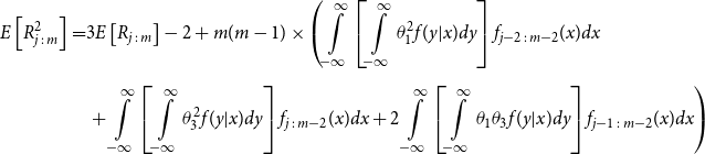 \begin{align}E\left[R_{j\,:\,m}^2\right]= & 3E\left[R_{j\,:\,m}\right] - 2 + m(m-1)\times \left(\int\limits_{-\infty}^{\infty}\left[\int\limits_{-\infty}^{\infty} \theta_1^2 f(y\vert x)dy\right] f_{j-2\,:\,m-2}(x)dx\right.\nonumber\\[5pt]& \left. + \int\limits_{-\infty}^{\infty}\left[\int\limits_{-\infty}^{\infty} \theta_3^2 f(y\vert x)dy\right] f_{j\,:\,m-2}(x)dx + 2 \int\limits_{-\infty}^{\infty}\left[\int\limits_{-\infty}^{\infty} \theta_1\theta_3 f(y\vert x)dy\right] f_{j-1\,:\,m-2}(x)dx \right)\end{align}
In the case of bivariate uniform distribution of (U,V), we have
 \begin{align*} E\left[R_{j\,:\,m}^2\right]=\, & 3 E\left[R_{j\,:\,m}\right] - 2 + m(m-1) \times \left(\int\limits_0^1 \left[\int\limits_0^1 \big(C(u,v)\big)^2 c(u,v) dv\right]f_{U_{j-2\,:\,m-2}}(u)du\right.\nonumber \\ & + \int\limits_0^1 \left[\int\limits_0^1 \big(v - C(u,v)\big)^2 c(u,v) dv\right]f_{U_{j\,:\,m-2}}(u)du\nonumber \\ & \left. +\, 2 \int\limits_0^1 \left[\int\limits_0^1 C(u,v)\big(v - C(u,v)\big) c(u,v) dv\right]f_{U_{j - 1\,:\,m-2}}(u)du \right) \\\nonumber\end{align*}

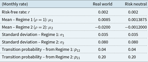

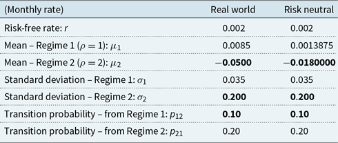
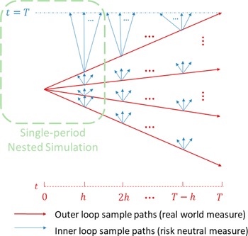
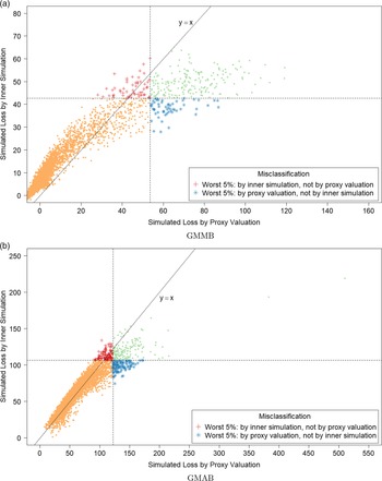


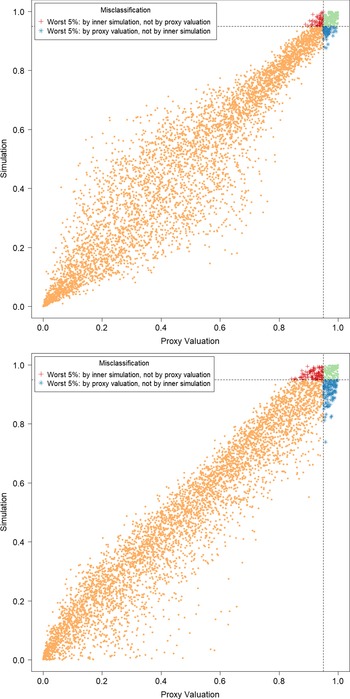

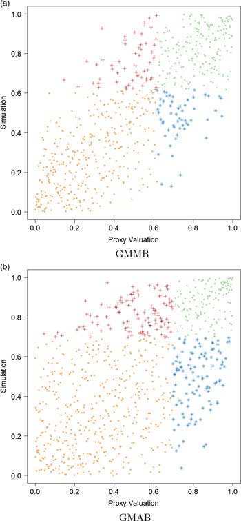


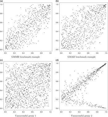

 Open access