


Introduction
Many of the world’s largest terrestrial mammals disappeared during the late Quaternary (Roberts et al. Reference Roberts, Flannery, Ayliffe, Yoshida, Olley, Prideaux, Laslett, Baynes, Smith, Jones and Smith2001; Wroe and Field Reference Wroe and Field2006; Barnosky et al. Reference Barnosky, Koch, Feranec, Wing and Shabel2004; Grayson Reference Grayson2007; Wroe et al. Reference Wroe, Field, Archer, Grayson, Price, Louys, Faith, Webb, Davidson and Mooney2013). In Sahul, 14 mammalian genera, approximately 88 species, and all taxa >100 kg went extinct sometime between middle and late Pleistocene times (Wroe et al. Reference Wroe, Field, Archer, Grayson, Price, Louys, Faith, Webb, Davidson and Mooney2013). Proportionally, Sahul (Pleistocene Australia–New Guinea) suffered the greatest loss of megafauna compared with other continents (Wroe et al. Reference Wroe, Field, Archer, Grayson, Price, Louys, Faith, Webb, Davidson and Mooney2013). Long-running debates about cause and effect in the extinction process have produced no clear consensus on primary causative factors and suffer from the fact that relatively little is known about the ecology of most extinct species. Current explanatory narratives include overhunting (e.g., Roberts et al. Reference Roberts, Flannery, Ayliffe, Yoshida, Olley, Prideaux, Laslett, Baynes, Smith, Jones and Smith2001; Prideaux et al. Reference Prideaux, Ayliffe, DeSantis, Schubert, Murray, Gagan and Cerling2009; Saltré et al. Reference Saltré, Rodríguez-Rey, Brook, Johnson, Turney, Alroy, Cooper, Beeton, Bird, Fordham and Gillespie2016), indirect effects of landscape modification (e.g., fire-stick farming by aboriginal people; Miller et al. Reference Miller, Fogel, Magee, Gagan, Clarke and Johnson2005), and impacts of long-term climate change (Price and Webb Reference Price and Webb2006; Wroe and Field Reference Wroe and Field2006; Faith and O’Connell Reference Faith and O’Connell2011; Price et al. Reference Price, Webb, Zhao, Feng, Murray, Cooke, Hocknull and Sobbe2011; Wroe et al. Reference Wroe, Field, Archer, Grayson, Price, Louys, Faith, Webb, Davidson and Mooney2013; Dortch et al. Reference Dortch, Cupper, Grun, Harpley, Lee and Field2016). Any new information about the dietary habits of the Pleistocene fauna may improve understanding of their potential vulnerabilities to adverse climatic conditions and may clarify habitat preferences of these extinct taxa.
There have been few opportunities to study the ecology of megafauna taxa, as many species are represented by only a few elements and sometimes are known from only one or two localities (see Prideaux et al. Reference Prideaux, Long, Ayliffe, Hellstrom, Pillans, Boles, Hutchinson, Roberts, Cupper, Arnold, Devine and Warburton2007). One exception is the giant short-faced kangaroo Procoptodon. Using similar methods to those implemented here, the 2- to 3-m-tall Procoptodon was identified as a C4 browser of Atriplex (saltbush), apparently preferring the “tough chenopod leaves and stems,” while also requiring access to free water (Prideaux et al. Reference Prideaux, Ayliffe, DeSantis, Schubert, Murray, Gagan and Cerling2009).
Isotopic data and dental microwear studies can be useful indicators of mammalian diets at different times in the mid–late Pleistocene. Insights into dietary preferences as revealed in these studies will assist in helping to understand the potential impacts of climate and environmental change on individual species, particularly the vulnerability of large herbivores to long-term climatic deterioration. We know of no well-dated faunal sequences during the late Pleistocene on mainland Australia, apart from Cuddie Springs, that have an in situ paleoenvironmental record documenting local vegetation and thus enable a direct correlation of environmental setting with the dietary habits of now extinct fauna. In this study, geochemical and dental microwear texture analyses (DMTA) were integrated to assess the environmental setting and dietary ecology of mammalian megafaunal communities from two concentrated, fossil bone horizons at Cuddie Springs: one from the middle Pleistocene dated to between ~570–350 Ka, and the second from a period when megafauna were in decline, ~40–30 Ka (see Field et al. Reference Field, Wroe, Trueman, Garvey and Wyatt-Spratt2013).
Site Setting and Paleoenvironmental History
Present-day Cuddie Springs is located in southeastern Australia on the semiarid riverine plains of northwestern New South Wales (Field and Dodson Reference Field and Dodson1999). It is an ancient ephemeral lake in a landscape of low relief and has been a low-energy depositional environment for hundreds of millennia. A treeless pan near the center of the lake fills after local rainfall and can take months to dry. Since the lake formed, the local environment has been primarily dominated by chenopod shrubland with scattered trees (Field et al. Reference Field, Dodson and Prosser2002). However, in the lead-up to the last glacial maximum (LGM, marine isotope stage 3), there was a shift to grasslands before the re-establishment of chenopod shrublands post-LGM (Field et al. Reference Field, Dodson and Prosser2002).
Cuddie Springs has been the subject of archaeological and prearchaeological excavations for more than two decades (Dodson et al. Reference Dodson, Fullagar, Furby, Jones and Prosser1993; Field et al. Reference Field, Wroe, Trueman, Garvey and Wyatt-Spratt2013). A stratified sequence of lacustrine clays and silts encloses a faunal record that could extend to nearly 1 Myr (Field and Dodson Reference Field and Dodson1999; Grün et al. Reference Grün, Eggins, Aubert, Spooner, Pike and Müller2010). At approximately 2 m below the ground surface, there is a discrete concentration of megafaunal bone approximately 20 cm deep (stratigraphic unit 9 [SU9]; Supplementary Fig. 1; Field and Dodson Reference Field and Dodson1999; Trueman et al. Reference Trueman, Field, Dortch, Charles and Wroe2005; Field and Wroe Reference Field and Wroe2012). A number of isolated tooth samples (n=5) from SU9 were analyzed using ESR/U-series and returned ages between 569±80 Ka and 347±55 Ka (Grün et al. Reference Grün, Eggins, Aubert, Spooner, Pike and Müller2010; sample numbers include 2028, 2055, 2058-60; note: these samples were incorrectly noted as occurring during SU8B in Grün et al. Reference Grün, Eggins, Aubert, Spooner, Pike and Müller2010). Grün et al. (Reference Grün, Eggins, Aubert, Spooner, Pike and Müller2010) present the age of SU9 as a weighted average mean of ca. 400 Ka, but omit why the dates were averaged in this way (note: we do list the average date in relevant tables and figures). The broad age range noted above encompasses three glacial cycles. The range of electron spin resonance (ESR)/U-series ages reflects the uncertainties in the dating method. In contrast to the wide age ranges resulting from ESR/U-series, geomorphological, geochemical, and taphonomic studies instead indicate that the bones in SU9 were deposited over a relatively short time period, possibly tens or hundreds of years rather than thousands (Field et al. Reference Field, Fullagar and Lord2001, Reference Field, Fillios and Wroe2008, Reference Field, Wroe, Trueman, Garvey and Wyatt-Spratt2013). The bones in SU9 accumulated in a low-energy environment, as indicated by the fine-grained lacustrine sediments, the articulated and separated articulated skeletal elements, and the pollen data (Field et al. Reference Field, Fillios and Wroe2008; and discussed below). An analysis of the faunal assemblage established that the bones were not weathered or abraded, and the rare earth elements (REE) study also indicated internal consistency (Trueman et al. Reference Trueman, Field, Dortch, Charles and Wroe2005). Notably, many of the elements from SU9 displayed damage by crocodiles, and more than 200 isolated crocodile teeth (predominantly Pallimnarchus sp.) were identified (J. H. Field and J. Garvey, unpublished data).
Two pollen samples were analyzed from the SU9 unit. Pollen preparations were carried out in the clean pollen preparation laboratory in the Institute of Earth Environment in Xi’an, China. The abundance of pollen and spores differed a little between the samples, but both samples were dominated by Chenopodeaceae (53–67%), with Poaceae (19 and 5%), Asteraceae (about 6%), and Casuarina (12–13%) also present. Many other taxa were represented in small amounts (<2–5%). These pollen data indicate that at the time of formation of SU9, the local environment was a saltbush plain with grasses, herbs, and scattered trees. The Casuarina component was probably from the immediate lake surrounds, growing adjacent to the ephemeral waterhole. Cyperaceae and aquatic taxa abundances were calculated outside the pollen sum. Cyperaceae were abundant at 19–36%, along with Myriophyllum (25 and 5%); both these taxa grow in still or slow-moving water bodies. Azolla spores (a small floating freshwater fern that grows in still, shallow freshwater; >50%) with abundant Azolla glochidia were also present. These pollen spores are consistent with a marshy environment and perhaps with periodic standing water, conditions not dissimilar from those found in the SU6B sequence.
Two sequential stratigraphic units (SU6A, SU6B; Supplementary Fig. 1), between ca. 1.7–1.05 m depth, contain discrete accumulations of artifactual stone interleaved with bone of extant and extinct species (Field and Dodson Reference Field and Dodson1999; Fillios et al. Reference Fillios, Field and Charles2010). SU6 was dated using ESR, optically stimulated luminescence (OSL), and radiocarbon techniques, with ages of >40 Ka to ~30 Ka (Field et al. Reference Field, Fullagar and Lord2001, Reference Field, Wroe, Trueman, Garvey and Wyatt-Spratt2013; Trueman et al. Reference Trueman, Field, Dortch, Charles and Wroe2005; Grün et al. Reference Grün, Eggins, Aubert, Spooner, Pike and Müller2010). The sediments in SU6B consist of silts and clays, with ped formation and fine plant roots throughout, consistent with the geomorphological interpretation as a swamp. As such, the fine plant roots are likely to be the same age as the deposit. SU6B was formed during waterlogged conditions, either as a shallow, still water body or as a marshy deposit (Field et al. Reference Field, Dodson and Prosser2002). The faunal remains show little to no weathering, with no evidence of abrasion; are extremely fragile; and are mostly complete, with some elements preserved in anatomical order, for example, a Diprotodon optatum mandible and numerous postcranial elements of Genyornis newtoni (Wroe et al. Reference Wroe, Field, Fullagar and Jermin2004; Fillios et al. Reference Fillios, Field and Charles2010; Field et al. Reference Field, Wroe, Trueman, Garvey and Wyatt-Spratt2013).
The Cuddie Springs investigations have been widely published with detailed descriptions of the in situ fossils and artifacts (as described earlier), yet the integrity of the site has been questioned on the basis of the OSL and ESR analyses (Roberts et al. Reference Roberts, Flannery, Ayliffe, Yoshida, Olley, Prideaux, Laslett, Baynes, Smith, Jones and Smith2001; Grün et al. Reference Grün, Eggins, Aubert, Spooner, Pike and Müller2010; Supplementary Fig. 1; but see Field Reference Field2006; Field et al. Reference Field, Fillios and Wroe2008, Reference Field, Wroe, Trueman, Garvey and Wyatt-Spratt2013). The ESR analyses for SU6 (Grün et al. Reference Grün, Eggins, Aubert, Spooner, Pike and Müller2010) produced, in some cases, ages that were considerably older than those produced with the OSL or radiocarbon analyses (also see Field et al. Reference Field, Fullagar and Lord2001). The Roberts et al. (Reference Roberts, Flannery, Ayliffe, Yoshida, Olley, Prideaux, Laslett, Baynes, Smith, Jones and Smith2001) OSL study identified multiple age populations from the single-grain analysis (but see Field and Fullagar Reference Field and Fullagar2001; Field et al. Reference Field, Fillios and Wroe2008, Reference Field, Wroe, Trueman, Garvey and Wyatt-Spratt2013). Stratigraphic disturbance was forwarded as the most likely explanation by these authors, yet other studies of single-grain OSL dating have routinely identified multiple age populations, and the interpretation of disturbance invoked by Roberts et al. (Reference Roberts, Flannery, Ayliffe, Yoshida, Olley, Prideaux, Laslett, Baynes, Smith, Jones and Smith2001) is rarely if ever interpreted this way (see Boulter et al. Reference Boulter, Bateman and Carr2006; Cosgrove et al. Reference Cosgrove, Field, Garvey, Brenner-Coltrain, Goede, Charles, Wroe, Pike-Tay, Grun, Aubert, Lees and O’Connell2010). Gillespie and Brook (Reference Gillespie and Brook2006: p. 9) also assert that the bones from Cuddie Springs (SU6) are “fossil rather than archaeological,” inferring that bones and stone tools were not contemporaneous. These interpretations ignore the published results of systematic stratigraphic studies undertaken over two decades (e.g., Field and Dodson Reference Field and Dodson1999; Field et al. Reference Field, Fullagar and Lord2001, Reference Field, Fillios and Wroe2008, Reference Field, Wroe, Trueman, Garvey and Wyatt-Spratt2013). Importantly, for the scenarios proposed by Grun et al. (2010) and Gillespie and Brook (Reference Gillespie and Brook2006) to have any credibility, the REE work of Trueman et al. (Reference Trueman, Field, Dortch, Charles and Wroe2005) had to be discredited. Grün et al. (Reference Grün, Eggins, Aubert, Spooner, Pike and Müller2010: p. 608) then concluded that Trueman et al. (Reference Trueman, Field, Dortch, Charles and Wroe2005) were analyzing “surface coatings and/or detrital material contained in cracks and pores.”
Trueman et al. (Reference Trueman, Field, Dortch, Charles and Wroe2005) were explicit in the description of their methodology and their approach, the salient points being: (1) the outer layers of bone were removed before sampling; (2) REEs have a strong affinity for apatite; and (3) bones with the highest U:Th ratios had the lowest REE content, demonstrating that REEs were associated with apatite (see discussion in Field et al. [Reference Field, Wroe, Trueman, Garvey and Wyatt-Spratt2013: p. 84]). Grün et al. (Reference Grün, Eggins, Aubert, Spooner, Pike and Müller2010) also constructed a scenario in which bone, stone, and charcoal were deposited at different times, the bones being “transported laterally” to this location by an unspecified mechanism from an unidentified source. Furthermore, these authors suggested that there was a “basin” formed at the lake center, with the larger lake floor at or near present-day levels. Grün et al. (Reference Grün, Eggins, Aubert, Spooner, Pike and Müller2010) further argue that these different levels produce an incline down which the bones would move, presumably for both SU6 and SU9. Gillespie and Brook (Reference Gillespie and Brook2006: p. 9) constructed another scenario, in which the animals, archaeology, and charcoal all accumulated by different mechanisms: “macro charcoal was transported to the site and later redeposited by floods.… European cattle farming significantly disturbed the claypan deposits.” Significantly, there is no empirical evidence supporting any of these assertions. Gillespie and Brook (Reference Gillespie and Brook2006) also try to reconcile the REE data (Trueman et al. Reference Trueman, Field, Dortch, Charles and Wroe2005) by suggesting that the local fauna died elsewhere, thus suggesting that all of the faunal remains were transported some distance in one episode. The various site formation processes forwarded by these authors require massive reworking and a demonstration of major landscape remodeling (not given) and notably have no support in the taphonomic, geomorphological, or archaeological studies undertaken to date (e.g., Trueman et al. Reference Trueman, Field, Dortch, Charles and Wroe2005; Fillios et al. Reference Fillios, Field and Charles2010; Field et al. Reference Field, Fullagar and Lord2001, Reference Field, Fillios and Wroe2008, Reference Field, Wroe, Trueman, Garvey and Wyatt-Spratt2013). For these reasons we reject the proposal that the site has been reworked, largely because there is no evidence to support this contention, while there is a significant amount of data contradicting these claims (e.g., Trueman et al. Reference Trueman, Field, Dortch, Charles and Wroe2005; Fillios et al. Reference Fillios, Field and Charles2010; Field et al. Reference Field, Fullagar and Lord2001, Reference Field, Fillios and Wroe2008, Reference Field, Wroe, Trueman, Garvey and Wyatt-Spratt2013).
Notably, the relative dating methods (ESR and OSL) used at Cuddie Springs have been applied to other Sahul sites—in particular Lake Mungo, NSW, and Devil’s Lair in Western Australia—with interpretations in direct contrast to Cuddie Springs (Thorne et al. Reference Thorne, Grün, Mortimer, Spooner, Simpson, McCulloch, Taylor and Curnoe1999; Turney et al. Reference Turney, Bird, Fifield, Roberts, Smith, Dortch, Grun, Lawson, Ayliffe, Miller, Dortch and Cresswell2001). The ESR estimates in these cases were thousands of years older than those obtained by other methods, just like Cuddie Springs, but the ESR dates were subsequently excluded from consideration at those sites (e.g., Bowler et al. Reference Bowler, Johnston, Olley, Prescott, Roberts, Shawcross and Spooner2003). We would argue, then, that for Grün et al (Reference Grün, Eggins, Aubert, Spooner, Pike and Müller2010) to maintain that the ESR dates are more reliable than the consensus of dates using other methods (OSL, 14C) at Cuddie Springs, they would need to demonstrate that their methods are not subject to the same sort of systematic error observed elsewhere. Similar conclusions were drawn from an OSL study undertaken by Roberts and colleagues (2001) at Cuddie Springs, in which multiple age populations were identified in the single-grain OSL data, and the authors subsequently concluded the site to have significant sediment disturbance. A similar pattern of multiple age populations was determined for a Tasmanian study of megafauna (Turney et al. [Reference Turney, Flannery, Roberts, Reid, Fifield, Higham, Jacobs, Kemp, Colhoun, Kalin and Ogle2008] and discussion in Cosgrove et al. [Reference Cosgrove, Field, Garvey, Brenner-Coltrain, Goede, Charles, Wroe, Pike-Tay, Grun, Aubert, Lees and O’Connell2010: p. 2497]); however, some of these age populations were “omitted for clarity,” and an age of ~45 Ka was used instead. While further work is needed to better standardize the treatment of OSL data, there is still much that can be learned from the sites mentioned earlier. For this reason we continue to study megafauna and their paleoecology based on data at hand and the accumulated wealth of published information about the Cuddie Springs site.
Paleoecological Proxies
The Sahul megafauna suite included a diversity of marsupials, whose potential diet may have included C3 and C4 grasses and C3 and C4 trees/shrubs. Carbon isotope studies of fossil fauna can help identify the isotopic signatures of these dietary food sources (e.g., Cerling et al. Reference Cerling, Harris, MacFadden, Leakey, Quade, Eisenmann and Ehleringer1997; Prideaux et al. Reference Prideaux, Ayliffe, DeSantis, Schubert, Murray, Gagan and Cerling2009). When combined with dental microwear analyses (e.g., Prideaux et al. Reference Prideaux, Ayliffe, DeSantis, Schubert, Murray, Gagan and Cerling2009), this approach can clarify long-term dietary trends in regions that contain a mixture of floral resources. The multiproxy approach implemented here provides a robust framework to clarify the dietary behavior of mammals. It is important to note that these proxy methods record diet during different times in an animal’s life. Stable isotopes record diet and climate via carbon and oxygen isotopes, respectively, during the time of mineralization (e.g., Cerling et al. Reference Cerling, Harris, MacFadden, Leakey, Quade, Eisenmann and Ehleringer1997; Passey and Cerling Reference Passey and Cerling2002), while dental microwear records diet over the past few days to weeks of an animal’s life (e.g., Grine Reference Grine1986). Here, we implemented these methods to investigate the dietary ecology of the mid- and late Pleistocene marsupial megafauna from Cuddie Springs.
Carbon isotope values from the tooth enamel of medium- to large-sized herbivorous marsupials can reflect food sources (i.e., modern plant values) when accounting for an enrichment factor of ~13.0‰ (Prideaux et al. Reference Prideaux, Ayliffe, DeSantis, Schubert, Murray, Gagan and Cerling2009) plus an additional ~1.5‰ due to increased atmospheric CO2 (fossil fuel burning over the past two centuries; Friedli et al. Reference Friedli, Lötscher, Oeschger, Siegenthaler and Stauffer1986; Marino et al. Reference Marino, McElroy, Salawitch and Spaulding1992; Cerling et al. Reference Cerling, Harris, MacFadden, Leakey, Quade, Eisenmann and Ehleringer1997). Thus, δ13C enamel values ≤−9‰ reflect a predominantly C3 diet, whereas values ≥−3‰ indicate a predominantly C4 diet. Further, more negative δ13C values can also suggest consumption of C3 vegetation within denser forests than more positive δ13C values (van der Merwe and Medina Reference van der Merwe and Medina1989; Cerling et al. Reference Cerling, Hart and Hart2004; DeSantis and Wallace Reference DeSantis and Wallace2008; DeSantis Reference DeSantis2011). Variation in stable isotope values within individual teeth have the potential to reveal seasonal differences in diet via carbon isotopes and changes in temperature, and/or precipitation/humidity via oxygen isotopes, respectively (e.g., Fraser et al. Reference Fraser, Grün, Privat and Gagan2008; Brookman and Ambrose Reference Brookman and Ambrose2012). Additionally, oxygen isotope values from modern Macropus tooth enamel are highly correlated with relative humidity and precipitation, ideally suited for tracking changes in aridity over time (Murphy et al. Reference Murphy, Bowman and Gagan2007; Prideaux et al. Reference Prideaux, Long, Ayliffe, Hellstrom, Pillans, Boles, Hutchinson, Roberts, Cupper, Arnold, Devine and Warburton2007; Burgess and DeSantis Reference Burgess and DeSantis2013).
An important adjunct to isotope studies is DMTA, specifically the three-dimensional study of microwear textures resulting from the processing of food. Dental microwear attributes such as complexity and anisotropy (see “Materials and Methods”) can distinguish extant grazers from browsers (e.g., Ungar et al. Reference Ungar, Merceron and Scott2007; Prideaux et al. Reference Prideaux, Ayliffe, DeSantis, Schubert, Murray, Gagan and Cerling2009; Scott Reference Scott2012), allowing for dietary behavior to be revealed beyond geochemical designations. This semiautomated method quantifies surface features in three dimensions using scale-sensitive fractal analysis, a major advance over prior microwear methods that instead required human observers to count pits and scratches from two-dimensional images, and subsequently minimizes observer biases (Ungar et al. Reference Ungar, Brown, Bergstrom and Walker2003; Scott et al. Reference Scott, Ungar, Bergstrom, Brown, Grine, Teaford and Walker2005; DeSantis et al. Reference DeSantis, Scott, Schubert, Donohue, McCray, Van Stock, Wilburn, Greshko and O’Hara2013).
Materials and Methods
Stable Isotope Analyses
Geochemical bulk (n=83) and serial samples (n=89) of tooth enamel were extracted from systematically excavated faunal material from Cuddie Springs, housed in the publicly accessible collections of the Australian Museum (see Supplementary Tables 1 and 5 for all specimen numbers and associated data). All sampled teeth were drilled with a low-speed dental-style drill and carbide dental burrs (<1 mm burr width). Bulk samples were taken parallel to the growth axis of the tooth, while serial samples were taken perpendicular to the growth axis. Enamel powder was pretreated with 30% hydrogen peroxide for 24 h and 0.1 N acetic acid for 12 h to remove organics and secondary carbonates, respectively (Koch et al. Reference Koch, Tuross and Fogel1997; DeSantis et al. Reference DeSantis, Feranec and MacFadden2009). These samples (~1 mg per sample) were then run on a VG Prism stable isotope ratio mass spectrometer with an in-line ISOCARB automatic sampler in the Department of Geological Sciences at the University of Florida. The analytical precision is ±0.1‰, based on replicate analyses of samples and standards (NBS 19). Stable isotope data were normalized to NBS 19 and are reported in conventional delta (δ) notation for carbon (δ13C) and oxygen (δ18O), where δ13C (parts per mil, ‰)=[(R sample/R standard) − 1]*1000, and R=13C/12C; and, δ18O (parts per mil, ‰)=[(R sample/R standard) − 1]*1000, and R=18O/16O; and the standard is VPDB (Pee Dee Belemnite, Vienna Convention; Coplen Reference Coplen1994). All stable isotopes (carbon and oxygen) are from the carbonate portion of tooth enamel hydroxylapatite.
Dental Microwear Texture Analyses
Dental microwear replicas of all extant and fossil taxa (n=90) were prepared by molding and casting using polyvinylsiloxane dental impression material and Epotek 301 epoxy resin and hardener, respectively. Modern faunal specimens were examined in publicly accessible collections housed in the Australian Museum, Museum Victoria, and the Western Australian Museum (see Supplementary Table 13 for all specimen numbers and associated data). DMTA using white-light confocal profilometry and scale-sensitive fractal analysis (SSFA), was performed on all replicas of bilophodont teeth that preserved antemortem microwear, similar to prior work (Ungar et al. Reference Ungar, Brown, Bergstrom and Walker2003, Reference Ungar, Merceron and Scott2007; Scott et al. Reference Scott, Ungar, Bergstrom, Brown, Grine, Teaford and Walker2005; Prideaux et al. Reference Prideaux, Ayliffe, DeSantis, Schubert, Murray, Gagan and Cerling2009; Scott Reference Scott2012; DeSantis et al. Reference DeSantis, Schubert, Scott and Ungar2012, Reference DeSantis, Scott, Schubert, Donohue, McCray, Van Stock, Wilburn, Greshko and O’Hara2013; Haupt et al. Reference Haupt, DeSantis, Green and Ungar2013; Donohue et al. Reference Donohue, DeSantis, Schubert and Ungar2013; DeSantis and Haupt Reference DeSantis and Haupt2014). Vombatids were not included in DMTA, because their tooth morphology is not analogous to the extant and extinct marsupials here examined.
All specimens were scanned in three dimensions in four adjacent fields of view for a total sampled area of 204×276 µm2. All scans were analyzed using SSFA software (ToothFrax and SFrax, Surfract Corporation, www.surfrait.com) to characterize tooth surfaces according to the variables of complexity (Asfc) and anisotropy (epLsar). Complexity is the change in surface roughness with scale and is used to distinguish taxa that consume hard, brittle foods from those that eat softer/tougher ones (Ungar et al. Reference Ungar, Brown, Bergstrom and Walker2003, Reference Ungar, Merceron and Scott2007; Scott et al. Reference Scott, Ungar, Bergstrom, Brown, Grine, Teaford and Walker2005; Prideaux et al. Reference Prideaux, Ayliffe, DeSantis, Schubert, Murray, Gagan and Cerling2009; Scott Reference Scott2012; DeSantis et al. Reference DeSantis, Schubert, Scott and Ungar2012, Reference DeSantis, Scott, Schubert, Donohue, McCray, Van Stock, Wilburn, Greshko and O’Hara2013; Haupt et al. Reference Haupt, DeSantis, Green and Ungar2013; Donohue et al. Reference Donohue, DeSantis, Schubert and Ungar2013; DeSantis and Haupt Reference DeSantis and Haupt2014; DeSantis Reference DeSantis2016). Anisotropy is the degree to which surfaces show a preferred orientation, such as the dominance of parallel striations having more anisotropic surfaces—as is typical in grazers and consumers of tougher food items (Ungar et al. Reference Ungar, Brown, Bergstrom and Walker2003, Reference Ungar, Merceron and Scott2007; Prideaux et al. Reference Prideaux, Ayliffe, DeSantis, Schubert, Murray, Gagan and Cerling2009; Scott Reference Scott2012; DeSantis et al. Reference DeSantis, Scott, Schubert, Donohue, McCray, Van Stock, Wilburn, Greshko and O’Hara2013; DeSantis Reference DeSantis2016).
Statistical Analyses
All statistical analyses follow the same methods of a priori geochemical and DMTA analysis (Ungar et al. Reference Ungar, Brown, Bergstrom and Walker2003; DeSantis et al. Reference DeSantis, Feranec and MacFadden2009, Reference DeSantis, Scott, Schubert, Donohue, McCray, Van Stock, Wilburn, Greshko and O’Hara2013; Prideaux et al. Reference Prideaux, Ayliffe, DeSantis, Schubert, Murray, Gagan and Cerling2009). Specifically, all carbon and oxygen isotope values within the same locality were analyzed using analysis of variance and post hoc Fisher’s least significant difference (LSD) and Tukey’s honest significant difference multiple comparisons, as all relevant samples from taxa with adequate sample sizes had δ13C values that were normally distributed and of equal variance (Shapiro-Wilk and Levene’s tests, respectively). When like genera between localities were being compared, t-tests were used if isotopic values were normally distributed and of equal variance (comparison of δ13C values from SU6 and SU9); however, nonparametric tests (Mann-Whitney U-tests) were used when comparing like genera with unequal variance (i.e., δ18O values of Macropus from Cuddie Springs SU6 and SU9). Further, we compared the δ18O values of Macropus from Cuddie Springs with modern Macropus specimens from different climatic regimes (i.e., low, moderate, high rainfall; Prideaux et al. Reference Prideaux, Long, Ayliffe, Hellstrom, Pillans, Boles, Hutchinson, Roberts, Cupper, Arnold, Devine and Warburton2007) using the Kruskal-Wallis test and Dunn’s procedure for multiple comparisons (due to significant differences in variance between Macropus δ18O values, Levene’s test). Serial samples of both δ13C and δ18O values were compared using two-tailed t-tests. Furthermore, we compared the variability of individuals present during each stratigraphic unit by quantifying the absolute difference between an individual serial sample and the mean value for the same isotope and tooth and then comparing those differences (as opposed to the isotopic values) between SU6 and SU9 using two-tailed t-tests. The comparison undertaken here allows for individual isotopic variability to be assessed while removing any confounding effects that could result from comparing teeth with disparate δ13C or δ18O values.
DMTA variables are not normally distributed (Shapiro-Wilk tests, p<0.05 for DMTA variables for certain taxa); therefore, we used nonparametric statistical tests (Kruskal-Wallis) to compare differences among all taxa. Further, we used Dunn’s procedure (Dunn Reference Dunn1964) to conduct multiple comparisons (between extant and/or extinct taxa) absent of the Bonferroni correction. As the Bonferroni correction is meant to reduce the likelihood of false positives (type I errors) by taking into consideration the number of comparisons being made, it also increases the probability of false negatives (type II errors; Cabin and Mitchell Reference Cabin and Mitchell2000; Nakagawa Reference Nakagawa2004). Furthermore, we do not want the number of extant and/or extinct comparisons to affect statistical differences between taxa; thus, the Bonferroni correction is not appropriate for our comparisons.
Results and Discussion
Oxygen Isotopes and Paleoclimate
Macropus teeth are known to be ideal for examining changes in aridity, as bulk δ18O enamel values of modern specimens are highly correlated with relative humidity and precipitation (Murphy et al. Reference Murphy, Bowman and Gagan2007; Prideaux et al. Reference Prideaux, Long, Ayliffe, Hellstrom, Pillans, Boles, Hutchinson, Roberts, Cupper, Arnold, Devine and Warburton2007; Burgess and DeSantis Reference Burgess and DeSantis2013). Additionally, Macropus taxa living today acquire most of their water from vegetation (e.g., Dawson Reference Dawson1995; Nowak Reference Nowak1999; Dawson et al. Reference Dawson, McTavish and Ellis2004), consistent with other “evaporation-sensitive” taxa capable of tracking changes in water deficits (Levin et al. Reference Levin, Cerling, Passey, Harris and Ehleringer2006). Macropus δ18O bulk values from all horizons examined at Cuddie Springs are consistent with Macropus values from low rainfall regimes (Prideaux et al. Reference Prideaux, Long, Ayliffe, Hellstrom, Pillans, Boles, Hutchinson, Roberts, Cupper, Arnold, Devine and Warburton2007; Fig. 1A).
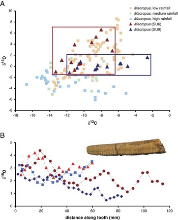
Figure 1 Stable isotope data indicative of relative aridity and seasonality. A, Stable carbon and oxygen isotope Macropus data of modern specimens from different rainfall regimes (Prideaux et al. Reference Prideaux, Long, Ayliffe, Hellstrom, Pillans, Boles, Hutchinson, Roberts, Cupper, Arnold, Devine and Warburton2007) and fossil specimens from Cuddie Springs. B, Serial oxygen isotope data of Diprotodon from individuals from prearchaeological (SU9, blue) and archaeological (SU6, red) horizons at Cuddie Springs shown with a serially sampled Diprotodon lower incisor.
SU9 was formed under less arid conditions than SU6, as inferred from lower δ18O mean values in Macropus (p=0.024, Mann-Whitney U-test; Fig. 1A, Supplementary Tables 1 and 2). Stable oxygen isotope values for SU9 are also significantly greater than those for extant kangaroos from high rainfall regimes, but are indistinguishable from kangaroos found in either medium or low rainfall regimes (Dunn’s procedure; Supplementary Tables 3 and 4).
Macropus δ18O values from SU6 are significantly greater than those for extant kangaroos from both high and medium rainfall regimes and only indistinguishable from kangaroos from low rainfall regimes (Dunn’s procedure; Supplementary Tables 3 and 4). Oxygen isotope values of Macropus during SU6 are also more variable (with a significantly higher variance, p<0.0001) than those from SU9. This high level of variability could result from a time-averaged accumulation of specimens, which included animals that died during normal and drought years—a situation often observed in modern times. For example, oxygen isotope data from extant quokkas (Setonix brachyurus) on Rottnest Island (an ~19 km2 island located ~20 km from Perth in Western Australia) during a period of a few years to decades (largely collected during the 1950s–1960s) yielded a δ18O range of 5.1‰ (see Supplementary Fig. 2 and Supplementary Table 5). The high level of δ18O variability was the result of fluctuating weather events, including droughts, and was produced over decades, even though significant time averaging (e.g., millennia) was absent. Kangaroo specimens should also be local and are unlikely to be from disparate geographic regions with distinctly different climates. Modern kangaroo home ranges are fairly limited: 90% of the kangaroos with the largest known home range, Macropus rufus, had home ranges of less than 10 km2 and never exceed dispersal distances of more than 13 km (Priddel et al. Reference Priddel, Wellard and Shepherd1988; Fisher and Owens Reference Fisher and Owens2000). Differences in mean oxygen isotope values (2.3‰) between SU6 and SU9 are significant (p=0.024). Shifts of this magnitude are similar to those of mammals observed during the Paleocene–Eocene thermal maximum, a dramatic period of warming ~55 Ma (Secord et al. Reference Secord, Bloch, Chester, Boyer, Wood, Wing, Kraus, McInerney and Krigbaum2012). Significant differences have also been observed between Pleistocene glacial and interglacial periods in Florida, where camelids, deer, and peccaries (all taxa present at both sites with samples sizes >5) exhibited increased mean δ18O values of ~2.4‰ (ranging from 1.8 to 2.9‰; DeSantis et al. Reference DeSantis, Feranec and MacFadden2009). For Cuddie Springs, SU6 formed during a period of enhanced aridity (ca. 41–27 Ka) and contrasts with a less arid climatic regime during SU9 (ca. 570–350 Ka).
Oxygen isotope values from serially sampled incisors of the largest known marsupial (~2700 kg) Diprotodon, indicate increased aridity and/or increased temperature during the formation of SU6, with significantly greater values at SU6 compared with SU9 (Fig. 1B, Supplementary Tables 6 and 7; p<0.0001, two-tailed t-test). Increased aridity is more likely, as Vostok and other Antarctic ice core records (Petit et al. Reference Petit, Jouzel, Raynaud, Barkov, Barnola, Basile, Bender, Chappellaz, Davis, Delaygue, Delmotte, Kotlyakov, Legrand, Lipenkov, Lorius, Pépin, Ritz, Saltzman and Stievenard2001; Jouzel et al. Reference Jouzel, Masson-Delmotte, Cattani, Dreyfus, Falourd, Hoffman, Minster, Nouet, Barnola, Chappellaz, Fischer, Gallet, Johnsen, Leuenberger, Loulergue, Luethi, Oerter, Parrenin, Raisbeck, Raynaud, Schilt, Schwander, Selmo, Souchez, Spahni, Stauffer, Steffensen, Stenni, Stocker, Tison, Werner and Wolff2007) indicate lower temperatures through SU6 relative to SU9 (Fig. 2A). Temperature and/or precipitation variability over the course of a year or more, as inferred from the amplitude of serial samples (assessed similar to Fraser et al. [Reference Fraser, Grün, Privat and Gagan2008] and Brookman and Ambrose [Reference Brookman and Ambrose2012]), does not noticeably change between units. The absolute difference between a given serial sample and the mean value for a given tooth is similar between SU6 and SU9 (0.6 and 0.5, respectively; p=0.941).

Figure 2 Geochemical data from the Vostok ice core (A) and the Cuddie Springs fauna (B). Vostok ice core data (Petit et al. Reference Petit, Jouzel, Raynaud, Barkov, Barnola, Basile, Bender, Chappellaz, Davis, Delaygue, Delmotte, Kotlyakov, Legrand, Lipenkov, Lorius, Pépin, Ritz, Saltzman and Stievenard2001) with temperature differences based on δ18O values noted through time (A); blue and red highlighted areas correspond to prearchaeological and archaeological horizons at Cuddie Springs (Trueman et al. Reference Trueman, Field, Dortch, Charles and Wroe2005; Fillios et al. Reference Fillios, Field and Charles2010; Grün et al. Reference Grün, Eggins, Aubert, Spooner, Pike and Müller2010). Tooth enamel stable carbon isotope values for the Cuddie Springs fauna through time (B), prearchaeological (SU9, ESR dates, Grün et al. Reference Grün, Eggins, Aubert, Spooner, Pike and Müller2010; blue) and archaeological (SU6, calibrated radiocarbon dates, Fillios et al. Reference Fillios, Field and Charles2010; red), carbon isotope values for individuals from corresponding temporal horizons are noted with distinct letters, indicating statistically different groups (i.e., taxa denoted with a b are not distinct from one another but are distinct from taxa with a, c, d, and e notation; Fisher’s LSD, p<0.05). P, prearchaeological; A, archaeological.
Enamel δ18O values of teeth from SU6 and SU9 further support other data sets (e.g., REE; Trueman et al. Reference Trueman, Field, Dortch, Charles and Wroe2005) that indicate an intact stratigraphic sequence at Cuddie Springs (Trueman et al. Reference Trueman, Field, Dortch, Charles and Wroe2005; Fillios et al. Reference Fillios, Field and Charles2010; Field et al. Reference Field, Wroe, Trueman, Garvey and Wyatt-Spratt2013). Specifically, δ18O bulk values of Macropus are significantly greater during SU6 compared with SU9—suggesting that these units are discrete—and are inconsistent with significant faunal mixing. Furthermore, the fairly narrow range of δ18O bulk values (2.8‰) of Macropus at SU9 are in agreement with a fairly rapid period of deposition, as also inferred from geomorphological studies. This range is also lower than δ18O ranges that occur in extant kangaroos over a period of a few decades (as evinced by quokkas, mentioned earlier; Supplementary Fig. 2). Oxygen isotope data from SU6 mammalian enamel are consistent with paleoenvironmental evidence for marked drying at ~50–45Ka (Bowler et al. Reference Bowler, Johnston, Olley, Prescott, Roberts, Shawcross and Spooner2003; Cohen et al. Reference Cohen, Nanson, Jansen, Jones and Jacobs2011) and, more broadly, longer-term climatic trends suggesting a trend of pronounced aridification since ~450Ka (Nanson et al. Reference Nanson, Price and Short1992; Kershaw et al. Reference Kershaw, Moss and van der Kaars2003; Wroe et al. Reference Wroe, Field, Archer, Grayson, Price, Louys, Faith, Webb, Davidson and Mooney2013).
Carbon Isotopes and Dietary Niches
During the formation of SU9 (ca. 570–350 Ka) the macropodids (Macropus, Protemnodon, and Sthenurus), diprotodontids (Diprotodon and Zygomaturus), and vombatid (Phascolonus) sampled in this study largely display disparate isotopic niches, with most taxa exhibiting significantly different mean δ13C values from other co-occurring mammals (Fig. 2B, Supplementary Tables 1, 8, and 9). Individual δ13C values range from −15 to −0.3‰, indicating the presence of dense forest–dwelling C3 consumers, mixed C3 and C4 consumers, and primarily C4 consumers. In contrast, megafauna from SU6 are largely indistinguishable from one another in δ13C values (Fig. 2B, Supplementary Tables 1, 7, and 10), with no individuals consuming primarily C4 resources (all individuals have δ13C values ≤−5.1‰). As water-stressed C3 plants can yield greater δ13C values with increased aridity (Tieszen Reference Tieszen1991), the proportion of C4 resources consumed by marsupials occurring during the formation of SU6 may be overestimated here. Thus, the effects of aridity on diet and subsequent reduction of C4 plants consumed during SU6 compared with SU9 may be even more pronounced.
Stable carbon isotopes also reveal considerable differences in dietary niches among macropodids, diprotodontids, and vombatids. During the formation of SU9 (ca. 570–350 Ka), mean δ13C values of resident taxa ranged from −13.5‰ in Sthenurus to −4.6‰ in Phascolonus (Supplementary Table 8). The rank order of all taxa sampled, from the most depleted in 13C (representing forest dwellers) to the most enriched in 13C (indicating the consumption of vegetation in more open regions, including potentially C4 grasses and/or C4 shrubs such as saltbush) is, as follows: Sthenurus, Protemnodon, Zygomaturus, Diprotodon, Macropus, and Phascolonus (Supplementary Table 8).
Sthenurus has significantly lower δ13C values from all other taxa in SU9, while Protemnodon has significantly lower δ13C values than Diprotodon, Macropus, and Phascolonus (Supplementary Table 9). Similarly, Zygomaturus has significantly lower δ13C values than Macropus and Phascolonus, while Diprotodon has significantly lower δ13C values than Phascolonus (Supplementary Table 9). Interestingly, and in contrast to prior morphological work suggesting that Sthenurus species may have consumed xeromorphic shrubs and were more open-country mixed feeders (Prideaux Reference Prideaux2004), these isotopic data suggest that Sthenurus preferred the densest vegetation available (van der Merwe and Medina Reference van der Merwe and Medina1989), in agreement with carbon and nitrogen isotope analyses of bone collagen (Gröcke Reference Gröcke1997). Specifically, Sthenurus consumed foliage in areas with denser canopies or understories than that consumed by other co-occurring macropods. While Protemnodon has greater δ13C values than Sthenurus, it had a preference for C3 browse, though was more of a mixed (C3/C4) feeder than was Sthenurus. Macropus consumed the greatest proportion of C4 resources of all macropodids analyzed, suggesting it consumed a large portion of C4 grasses and/or C4 shrubs such as saltbush. Further, the rank order of δ13C values of all macropodids is maintained from SU9 to SU6 (although Sthenurus is only represented by one sample; Supplementary Table 8, Supplementary Fig. 3). In SU6 Protemnodon had a significantly lower mean δ13C value than Macropus, Diprotodon, and Vombatus. Nonetheless, all macropods with sample sizes appropriate for analysis demonstrate a significant decline in δ13C values with increased aridity (p<0.05). Declining δ13C values are contrary to expectations, as increased aridity is likely to result in greater (i.e., water-stressed; Tieszen Reference Tieszen1991) δ13C values and/or an increase of C4 vegetation on the landscape (as seen in DeSantis et al. Reference DeSantis, Feranec and MacFadden2009). Significant declines in δ13C values, coupled with aridity, suggest that macropods were shifting their diets to compensate for changing climatic conditions. If C4 vegetation was less palatable during more arid conditions (either due to lower water content and/or increased salt content in the case of C4 shrubs like Atriplex), herbivorous megafauna may have been competing for a reduced suite of vegetative resources during SU6.
Both diprotodontids at Cuddie Springs (i.e., Zygomaturus and Diprotodon in SU9) had δ13C values suggesting consumption of both C3 and C4 resources. Despite Zygomaturus having a smaller body size than Diprotodon (e.g., Murray Reference Murray1991), isotopic data suggest they consumed similar dietary resources. The diet of Diprotodon at Cuddie Springs also varied seasonally; however, total δ13C variability per individual sampled is ≤3‰, indicating that Diprotodon did not switch from eating only C3 vegetation to only C4 vegetation (which would result in larger individual δ13C variability than 3‰; Supplementary Fig. 4, Supplementary Tables 6 and 7). Instead, Diprotodon had a diet with more subtle annual or semiannual differences. Interestingly, variability in serial carbon isotope samples compared with the mean value for a given tooth is significantly greater during SU6 when compared with SU9 (0.7 and 0.5, respectively; p=0.02). These data suggest that while mean δ13C bulk values of Diprotodon do not vary between stratigraphic units, individuals present during SU6 consumed more temporally variable diets than did individuals from SU9.
The vombatids Phascolonus (SU9) and Vombatus (SU6) consumed the greatest proportion of C4 resources of all Cuddie Springs taxa sampled. As extant members of the genus Vombatus consume primarily grasses (Nowak Reference Nowak1999; Triggs Reference Triggs2009), it is likely that the Cuddie Springs vombatids consumed C4 grasses during the formation of SU6 and SU9. Nonetheless, during SU6 Vombatus probably supplemented its diet with C3 resources, as these data suggest that none of the marsupials sampled from SU6 were specialized C4 consumers. The small amount of C4 flora consumed by SU6 Vombatus at Cuddie Springs, as inferred from δ13C values<−5.0‰, is consistent with the Miller et al. (Reference Miller, Fogel, Magee, Gagan, Clarke and Johnson2005) study, in which wombats (in addition to flightless birds) reduce their consumption of C4 vegetation during the late Pleistocene.
Dental Microwear Texture Analysis and Paleoecology
Modern vegetation around Cuddie Springs consists of semiarid woodland with a shrub understory including chenopods, grasses, and lignum (Field et al. Reference Field, Dodson and Prosser2002). As many chenopods are C4 plants, including the saltbush Atriplex, we cannot discern from isotopes alone whether the decline in C4 consumption reflects declining grass or saltbush consumption, though the pollen record for this period (SU6) does reflect a local shift to grasses from saltbush (Field et al. Reference Field, Dodson and Prosser2002). DMTA can distinguish between extant grazing and browsing macropods (Prideaux et al. Reference Prideaux, Ayliffe, DeSantis, Schubert, Murray, Gagan and Cerling2009) and in this study revealed differences between extant grazers (Macropus giganteus), grazers with a more varied diet (Macropus fuliginosus), browsers (Setonix brachyurus), and browsers with a more varied diet (Wallabia bicolor; Fig. 3; Arman and Prideaux Reference Arman and Prideaux2015). All identified fossil macropodid and diprotodontid taxa from Cuddie Springs (Macropus, Protemnodon, Sthenurus, Diprotodon, Palorchestes, Zygomaturus) yielded dental microwear textures indicative of browsing (low anisotropy, epLsar; high complexity, Asfc; Fig. 3, Supplementary Tables 11–14). All samples (except Palorchestes, which was excluded from statistical analyses due to small sample size) were indistinguishable in complexity (indicative of harder object feeding) from the extant swamp wallaby (W. bicolor; p>0.05). Further, these taxa are all significantly different (p<0.05) in both Asfc and epLsar from the extant obligate grazer Macropus giganteus.

Figure 3 DMTA values and photosimulations for extant (A–D) and extinct taxa (E–J) from Cuddie Springs. A scatter plot of dental microwear texture attributes of complexity (Asfc) and anisotropy (epLsar) of extant and extinct taxa. Extant taxa (open symbols, A–D); extinct taxa (solid symbols, E–J; P, prearchaeological; A, archaeological). Photosimulations of the following extant museum specimens are included: Macropus giganteus (A, MV-C24527), Macropus fuliginosus (B, WAM-M12229), Setonix brachyurus (C, WAM-M3543), and Wallabia bicolor (D, AM-M36793). Cuddie Springs photosimulations of prearchaeological (SU9) specimens include: Macropus (E, CS-1059), Protemnodon (F, CS-1069), Sthenurus (G, CS-1071), Palorchestes (H, CS-1049), Diprotodon (I, CS-1034), and Zygomaturus (J, CS-1044).
In contrast to disparate mean δ13C values of macropodids from SU9 and SU6 (Supplementary Fig. 2), all macropodids consumed a significant portion of woody or more brittle floral material. However, Protemnodon consumed more brittle material than Macropus (Fig. 3, Supplementary Table 12), as suggested by greater complexity (Asfc) values in the former. Furthermore, the Cuddie Springs Macropus are significantly different, in both complexity and anisotropy (epLsar), from the extant grazing kangaroo (Macropus giganteus; Supplementary Tables 12 and 13). Collectively, these data suggest that macropodids from Cuddie Springs consumed a broad range of floral resources and had disparate dietary niches. However, all macropodids likely consumed a greater amount of browse, including shrubs (e.g., saltbush, especially likely in taxa with elevated δ13C values and when considering the abundance of chenopods as supported by pollen data; Supplementary Figs. 5 and 6) than modern extant grazing kangaroos, as indicated by DMTA data (Fig. 3, Supplementary Tables 12–14).
Concluding Remarks
Collectively, DMTA data indicate that browsers dominated the Cuddie Springs fauna. Furthermore, C4 shrubs such as saltbush may have been a preferred component of the diet of some taxa, as has been suggested for the giant short-faced kangaroo, Procoptodon goliah (Prideaux et al. Reference Prideaux, Ayliffe, DeSantis, Schubert, Murray, Gagan and Cerling2009). Importantly, our data demonstrate that these C4 consumers were restricted to predominantly C3 resources in the late Pleistocene. The long-term aridification trend identified in other paleoenvironmental records (Nanson et al. Reference Nanson, Price and Short1992; Kershaw et al. Reference Kershaw, Moss and van der Kaars2003; Cohen et al. Reference Cohen, Nanson, Jansen, Jones and Jacobs2011; Wroe et al. Reference Wroe, Field, Archer, Grayson, Price, Louys, Faith, Webb, Davidson and Mooney2013) may have reduced the availability of C4 resources at the times these fossil records were formed. During a climatic downturn, the potential of megafauna to consume C4 resources such as saltbush may have also been reduced, because of the need to increase water intake to compensate for increased salt consumption (as demonstrated by Prideaux et al. Reference Prideaux, Ayliffe, DeSantis, Schubert, Murray, Gagan and Cerling2009). If standing water and/or plant water were diminished at these times or competition (with crocodiles or other taxa) reduced access, saltbush (due to its high salt content) would become less palatable, thereby increasing competition for other plant resources.
Previous studies of C3 and C4 plant consumption, conducted on emu and Genyornis newtoni eggshell and mammalian tooth enamel (Miller et al. Reference Miller, Fogel, Magee, Gagan, Clarke and Johnson2005), have demonstrated similar declines in C4 resource consumption. The subsequent vulnerability of the large flightless bird, Genyornis newtoni, to deteriorating climate from around 50 Ka (Kershaw et al. Reference Kershaw, Moss and van der Kaars2003; Cohen et al. Reference Cohen, Nanson, Jansen, Jones and Jacobs2011) occurred during a period of very low human population densities across Sahul (Williams Reference Williams2013). A time-series analysis of the same eggshell data (Murphy et al. Reference Murphy, Williamson and Bowman2012) determined that changes in emu diet are better correlated with fluctuating Lake Eyre water levels (Kershaw et al. Reference Kershaw, Moss and van der Kaars2003; Cohen et al. Reference Cohen, Nanson, Jansen, Jones and Jacobs2011). As such, this interpretation contrasts markedly with the initial conclusion that attributed Genyornis decline to ecosystem disruption by the landscape burning of colonizing humans (Miller et al. Reference Miller, Fogel, Magee, Gagan, Clarke and Johnson2005), for which there is no empirical evidence for this region. Instead, data from Miller et al. (Reference Miller, Fogel, Magee, Gagan, Clarke and Johnson2005) as interpreted by Murphy et al. (Reference Murphy, Williamson and Bowman2012) suggest that increased aridity may have been a driving factor influencing bird and wombat dietary shifts (a reduction in C4 consumption, like we see at Cuddie Springs) and perhaps their eventual extinction.
The reduction of C4 resources consumed by marsupial herbivores during the formation of SU6 suggests that megafauna may have been subject to increased competition for similar resources. It contrasts with SU9, when a broader range of palatable vegetative resources and suitable niches could be partitioned. It is also clear that megafauna living during SU6 experienced more arid conditions compared with those occurring during the formation of SU9. These data, together with published climatic data, lend support to a climatic downturn in the lead-up to the LGM (Nanson et al. Reference Nanson, Price and Short1992; Kershaw et al. Reference Kershaw, Moss and van der Kaars2003; Cohen et al. Reference Cohen, Nanson, Jansen, Jones and Jacobs2011; Wroe et al. Reference Wroe, Field, Archer, Grayson, Price, Louys, Faith, Webb, Davidson and Mooney2013). The deteriorating climatic conditions that would have driven significant environmental reconfiguration during MIS3 may have strongly impacted the megafauna suite that persisted during the late Pleistocene in arid southeastern Sahul.
Acknowledgments
This work was supported by the National Science Foundation (EAR1053839 and FAIN1455198), the Australian Research Council (ARC LP211430 and DP05579230), the University of New South Wales, the University of Sydney, Oak Ridge Associated Universities Ralph E. Powe Junior Faculty Enhancement Award, and Vanderbilt University (including the Discovery Grant Program). We thank M. Fillios, J. Garvey, R. How, S. Ingleby, W. Longmore, K. Privat, K. Roberts, and C. Stevenson for contributions to the study and/or access to materials. Enormous gratitude is due to P. Ungar and J. Scott for initial access to and assistance with DMTA; J. Curtis for isotopic analysis; J. Olsson for the shadow drawings in Fig. 2B; and J. Roe for the Cuddie Springs map and section drawings. We are beholden to the Brewarrina Aboriginal Community; the Walgett Shire Council; the Johnstone, Currey, and Green families; and many volunteers for their support and assistance in the research at Cuddie Springs. Many thanks to Douglas and Barbara Green for facilitating access to the site. Thanks to I. Davidson, D. Fox, S. Mooney, R. Secord, and anonymous reviewers for comments on an earlier version of this article.
Supplementary Material
Data available from the Dryad Digital Repository: https://doi.org/10.5061/dryad.1s3d4


 Open access