


Introduction
Ice cores contain information on climatic and geochemical conditions of the past, because the isotopic and chemical composition of falling snow remains unchanged in glacier ice for long periods of time. However, the value of isotopic and chemical analysis is, of course, closely related to a knowledge of the age of the ice in question. This emphasizes the necessity for establishing a time versus depth relation.
Macroscopic stratigraphie studies have been used by many investigators on the upper strata of ice which are no more than a few hundred years old. However, the technique based on seasonal variation in light transmissivity (Reference LangwayLangway, 1967) might be used for ice several thousand years old (Reference JohnsenJohnsen and others, unpublished).
Another possible way of establishing a time scale along an ice core would seem to be the measurement of seasonal oscillations in the isotopic composition of the ice (Reference Epstein and SharpEpstein and Sharp, 1959) and counting isotopic maxima from the surface. However, various processes tend to diminish the isotopic gradients in snow and ice. For example, molecular diffusion in the solid ice, accelerated by the thinning of the layers, gradually obliterates the stable isotope oscillations that remain after firnification (Reference Johnsen and DansgaardJohnsen and Dansgaard, unpublished).
Four radioactive isotopes have been used for dating ice. Tritium (Reference AegerterAegerter and others, 1969) and 210Pb (Reference GoldbergGoldberg, 1963; Reference CrozazCrozaz and others, 1964; Reference Crozaz and LangwayCrozaz and Langway, 1966) reach only 100 years back in time. The other two, 32Si (Reference DansgaardDansgaard and others, 1966) and 14C (Reference ScholanderScholander and others, 1962), may be detected in 3 000 and 20 000–30 000 year-old ice, respectively, but both of these techniques require several tons of ice. The technique for sampling 14C from ice in situ, developed by Reference OeschgerOeschger and others (1967), might in the future be perfected to be applied to deep bore holes.
But at present a time scale for the Camp Century core must be based on calculations on a chosen flow model.
The Nye Model
Most of the previously evaluated flow models imply a uniform vertical strain-rate along any vertical line in an ice cap (Reference NyeNye, 1951, Reference Nye1957, Reference Nye1959). Furthermore, assuming that the horizontal velocity components are parallel and there is negligible melting at the bottom, Reference NyeNye (1963) expressed the ratio between the reduced and initial thicknesses, λ and λ H , of an annual layer (e.g. in cm of ice) by
y and H being its present and initial distance from the bed.
With this model, we get the change of λ per unit of time

τ being 1 year. Integration gives λ as a function of time

and from Equation (1) we get the depth of a layer age t formed at a height H above the bottom

Hence, the age of a layer (H−y) below surface (cf. Reference HaefeliHaefeli, 1961)

Figure 1 shows λ as a function of time (Equation (2)) for H = 1 400 m and λ H = 0.2 and 0.35 m. Paradoxically, the highest value of λ H corresponds to the thinnest layers after 5 000 years. The explanation is that, for a given value of H, the horizontal movement and, therefore, the vertical strain-rate will be the faster the higher the rate of accumulation.

Fig. 1. Thickness λ of an annual layer as a function of age t, according to the, Nye flow model. Initial thicknesses 0.35 and 0.20 m. Thickness of the ice sheet H = 1 400 m.
The Nye model describes the flow conditions at the bedrock by sliding and/or by rapid shear strain-rates being concentrated in a thin bottom layer (Reference NyeNye, 1963). However, at Camp Century the sliding is probably negligible, because the temperature at the bottom is as low as −13°C (Reference Hansen and LangwayHansen and Langway, 1966). Furthermore, the idea of relative motion being essentially concentrated in a thin bottom layer was advanced in view of the fact that the flow law of ice depends critically upon the temperature, at the same time as the temperature gradient at the bottom was assumed to be as high as 10°C/100 m (Reference NyeNye, 1959). However, at Camp Century the temperature gradient was later measured to be only 1.8°C/100 m (Reference Hansen and LangwayHansen and Langway, 1966). Consequently, Nye’s flow model is not necessarily applicable in the case of the Camp Century area.
Non-uniform Vertical Strain-rate Model
Another approach would be to assume, like Reference NyeNye (1963), that the horizontal velocity profile along a vertical line in the distance x from the ice divide may be written as
and also to calculate v x (y) by integrating Glen’s law (Reference Haefeli, 1961)

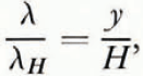
σ being the shear stress, k′ and n being constants that depend on the temperature and therefore on y. This integration is justificd only if the longitudinal strain-rate is small compared with the shear strain-rate at any y, which is only the case in the lower part of the ice sheet. Nevertheless, we consider Reference WeertmanWeertman’s (1968) calculation of Equation (5), shown as the full curve in Figure 2, as an improvement compared with calculations based on a uniform vertical strain-rate, because Weertman’s procedure accounts for the important fact, that v x (y) = 0 for y = 0. In this work, we use the simple approximation shown as the dashed curve in Figure 2, i.e. v x proportional to y from y = 0 to y = h, and v x independent of y from y = h to y = H or, in other words

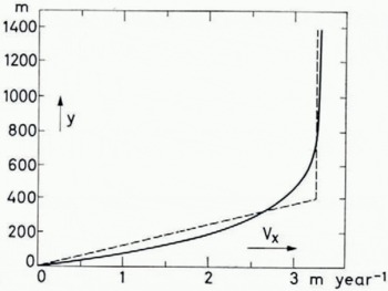
Fig. 2. Full curve: horizontal velocity profile calculated by integration of Glen’s law, assuming vx(0) = 0 and vx(H) = 3.3m year−1 (from Reference WeertmanWeertman, 1968). Dashed curve: adopted approximation.
The incompressibility of the ice is expressed by

and the vertical velocity component is calculated as

and, according to Equation (6)

For y = h:

For y = H:

Inserting Equations (8) and (9) into Equation (7) gives

which is shown in Figure 3 (cf. discussion on p. 217–18). The straight line in the upper range intersects the y-axis at y = h/2. Consequently, in the same range, h ≤ y ≤ H, we can use Nye’s model and Equations (1), (2) and (3), if H and y are replaced by


Fig. 3. Vertical velocity vy as a function of the distance y from the bottom. Dashed line: the Nye flow model; full curve: the flow model described on p. 217. The dashed curve close to the full curve corresponds to the horizontal velocity profile calculated by Reference WeertmanWeertman (1968); cf Fig. 2.
In the range 0 ≤ y ≤ h, Equation (10) gives

Integration over the intervals h→y and t h →t (t h being the age of ice at y = h given by Equation (12)) leads to

or

and from Equations (13) and (14)

Using the equations way back in time implies that H and λ H are independent of x and, furthermore, steady-state conditions in a broad sense, i.e. H, λ H and ice temperature T are constant in time.
The former assumption seems justified (i) by the direction of the movement at Camp Century being approximately parallel to the iso-accumulation curves in the area (Reference MockMock, 1968), and (ii) by the site of formation of even a 15 000 year old section of the core being barely more than 50 km from Camp Century (the surface velocity is 3.3 m/year (Mock, referred to by Reference WeertmanWeertman (1968)). As to the changes in the non-independent parameters, H, λ H and T, many thousand years back in time, it might be reasonable to assume lower λ H and T, but higher H during the glaciation. Lower λ H in that period would correspond to a closer packing of the annual layers, which, on the other hand, would be counteracted by slower thinning of the layers due to lower temperature (i.e. higher viscosity of the ice) and higher H. However, we have no means of verifying such assumptions, so all that we can do at present is to calculate the time scale by using the present constants and try, by other means, to check if and when an error enters (these remarks, of course, should also be considered in connection with the thinning of the Iayers (Fig. 3)).
The mean value of λ H over the last 100 years has been 0.35±0.03 m of ice, as shown by Reference Crozaz and LangwayCrozaz and Langway (1966) by the 210Pb method. The surface to bottom distance, H, was measured as 1 387.5 m in 1966 (Reference Hansen and LangwayHansen and Langway, 1966), corresponding to 1 367.5 m of ice in view of the low densities in the upper layers (personal communication from C. C. Langway, Jr.).
Thus, we can use Equations (12) and (15) with H = 1 367.5m, h = 400 m, λ H = 0.35m, and τ = 1 year. For t > 6 000 years, we can write
The result is shown by the full curves in Figures 4 and 5. According to the Nye model (dashed curve; Equation (4)), only the lowest few metres of ice should be more than 20 000 years old, whereas in our model the ice reaches this age 130 m above the bottom.

Fig. 4. Age of the ice in the Camp Century core as a function of the distance y from the bottom. y ≥ h. S is the 1966 surface (y = 1387.5 m) and S′ is the 1966 surface corrected for low densities in the upper layers (y′ = H = 1367.5 m of ice).

Fig. 5. Age of the ice in the Camp Century core as a function of the distance y from the bottom (1160 m ≥ y ≥ 20m) both on a logarithmic scale.
Experimental Evidence
The validity of the flow model described above has been checked in two independent ways. First, the flow model was used as a basis for calculating the temperature profile down the bore hole (Reference Dansgaard and JohnsenDansgaard and Johnsen, 1969). The result fitted the profile measured by Reference Hansen and LangwayHansen and Langway (1966) within ±0.6°C. The calculated temperature difference between surface and bottom deviated only 0.3°C from the measured difference. Using the Nye model, Reference WeertmanWeertman (1968) found a deviation of 2.7°C.
Secondly, when stable oxygen-isotope data for about 1 600 samples from the core were plotted against the age of the ice in our time scale (Fig. 6), they showed a variation which was in complete agreement with practically all known climatic changes within the last 70 000 of 100 000 years (for further details, cf. Reference DansgaardDansgaard and others, in press). The geochemical explanation for this is the fact that the isotopic composition of precipitation at high latitudes is mainly determined by the temperature of formation (Reference DansgaardDansgaard, 1954, Reference Dansgaard1964; Reference Gonfiantini and PicciottoGonfiantini and Picciotto, 1959), which causes seasonal isotopic oscillations in the ice strata, as well as long-period isotopic variations in phase with climatic changes.
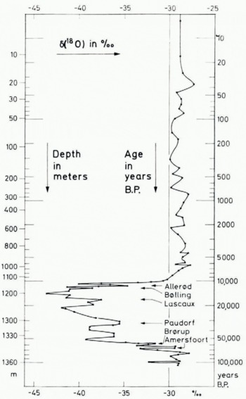
Fig. 6. The heavy oxygen isotope concentration, δ(18O), of sections of the Camp Century core versus the age of the ice (Equations (12) and (15)) plotted on a logarithmic scale to the right. The outer scale to the left gives the corresponding depth below the 1966 surface. The isotope data are given as relative deviation of the 18O/16O ratio from that of standard mean ocean water. (From Reference DansgaardDansgaard and others, unpublished.)
The agreement with other quite independent climatological estimates, covering nearly 100 000 years, leads us to the conclusion that the time scale and therefore our flow model is basically correct down to 30 or 35 m above the bottom. Below that level, the flow pattern is probably influenced by the irregular topography of the bottom, which is also indicated by visual observation of the lowest silty core sections.
Moreover, unless the influences of the various parameters, which determine the flow pattern, quite accidentally counterbalance each other (e.g. as outlined on p. 220), it would seem as if λ H and H have not deviated considerably from their present values in the Camp Century area.
One might ask how the time scale is influenced by the choice of h (cf. Fig. 2). To check this, we consider a horizon y = 209.0 m above the bottom. In our time scale (h = 400 m) the age is t209 = 12 000 years with an uncertainty of barely more than 1 %,Footnote * whereas, for h = 300 m (500 m), t209 would be 10 400 years b.p. (13 600 years b.p.). Thus, if f(y) is accepted in accordance with Equation (6), h must be very close to 400 m.
Acknowledgement
The authors are indebted to the Carlsberg Foundation, Copenhagen, for financial support.


