


1. Introduction
The foundational studies on multiphase electrohydrodynamics (EHD) can be traced back to the work of Rayleigh (Reference Rayleigh1882), who discovered that a charged drop exhibits instability and the ejection of satellite droplets from the cone of the droplet, a phenomenon known as Coulomb fission (Stuart Reference Stuart1985; Duft et al. Reference Duft, Achtzehn, Müller, Huber and Leisner2003; Fernández de la Mora Reference Fernández de la Mora2007). Subsequently, Taylor (Reference Taylor1964) discovered that, under a strong external electric field, a liquid cone would be stretched parallel to the field, generating jet streaming from the conical tip. The seminal review by Melcher & Taylor (Reference Melcher and Taylor1969) has generated considerable research interest in the field. In particular, Allan et al. (Reference Allan, Mason and Marion1962) found that a weakly conductive dielectric droplet subjected to an electric field not only deforms parallel to the field (prolate) but also deforms perpendicular to the field direction (oblate). Over the subsequent decades, continuous experimental (Ha & Yang Reference Ha and Yang2000; Reznik et al. Reference Reznik, Yarin, Theron and Zussman2004; Achtzehn et al. Reference Achtzehn, Müller, Duft and Leisner2005) and theoretical research (Stuart Reference Stuart1985; Reznik et al. Reference Reznik, Yarin, Theron and Zussman2004; Betelú et al. Reference Betelú, Fontelos, Kindelán and Vantzos2006) has provided new physical insights, establishing the foundation for wide application of multiphase EHD (Zhang et al. Reference Zhang, Wang, Wang, Li, Yu, Zhan, Huo, Wang and Xu2023). One of the most representative applications of multiphase EHD is electrospray mass spectrometry (Fenn et al. Reference Fenn, Mann, Meng, Wong and Whitehouse1989, Reference Fenn, Mann, Meng, Wong and Whitehouse1990), which contributed to Finn winning the Nobel Prize in Chemistry in 2002. In contrast to the theoretical and experimental advancements, numerical simulation research on multiphase EHD has progressed relatively slowly (Vlahovska Reference Vlahovska2019; Wagoner et al. Reference Wagoner, Vlahovska, Harris and Basaran2021). While Taylor, McEwan & de Jong (Reference Taylor, McEwan and de Jong1966) first proposed the leaky dielectric model (LDM) in their paper over 50 years ago, simulations specifically addressing Coulomb fission did not appear until 2008 (Collins et al. Reference Collins, Jones, Harris and Basaran2008).
Extensive research has been conducted on the prolate breakup of the droplets (Vlahovska Reference Vlahovska2019), especially for Coulomb fission (Fernández de la Mora Reference Fernández de la Mora2007). Rayleigh (Reference Rayleigh1882) predicted that instability occurs when the droplet carries a charge greater than  ${q_c} = 8{\rm \pi}\sqrt {\gamma \varepsilon R_0^3} $ ( ${R_0}$ is the initial radius of the droplet, $\varepsilon $ is dielectric permittivity, $\gamma $ is surface tension). Subsequent experiments (Bentley & Leal Reference Bentley and Leal1986; Karyappa, Deshmukh & Thaokar Reference Karyappa, Deshmukh and Thaokar2014) revealed that, besides the jetting from the tips, prolate deformation of droplets can result in various breakup outcomes, such as lobes breaking and open jets. Additionally, some experimental studies researched Coulomb fission for non-Newtonian droplets (Ha & Yang Reference Ha and Yang2000; Mandal & Chakraborty Reference Mandal and Chakraborty2017) and droplets containing surfactants (Eggleton, Tsai & Stebe Reference Eggleton, Tsai and Stebe2001; Luo et al. Reference Luo, Yan, Huang, Yang, Wang and He2017). Another interesting topic in Coulomb fission is the charge and mass loss of the droplet (Fernández de la Mora Reference Fernández de la Mora2007). Duft et al. (Reference Duft, Achtzehn, Müller, Huber and Leisner2003) first provided high-resolution experimental images for charged droplet Coulomb fission, indicating that the droplet's charge loss is approximately 33 % of the total charge, with a mass loss less than 1 %. A subsequent numerical study by Gawande, Mayya & Thaokar (Reference Gawande, Mayya and Thaokar2017) has confirmed this experimental discovery. Interest in Coulomb fission has sparked numerous numerical studies (Giglio et al. Reference Giglio, Gervais, Rangama, Manil, Huber, Duft, Müller, Leisner and Guet2008; Burton & Taborek Reference Burton and Taborek2011; Mandal & Chakraborty Reference Mandal and Chakraborty2017; Sengupta, Walker & Khair Reference Sengupta, Walker and Khair2017; Li et al. Reference Li, Pang, Sun, Sun, Qi, Li, Liu, Li, Wang and Zeng2023) aiming to simulate the droplet prolate breakup in an electric field. Collins et al. (Reference Collins, Jones, Harris and Basaran2008, Reference Collins, Sambath, Harris and Basaran2013) first proposed a scaling law for the radius of ejected droplets and the charge quantity in EHD tip streaming. Subsequently, Gawande, Mayya & Thaokar (Reference Gawande, Mayya and Thaokar2019, Reference Gawande, Mayya and Thaokar2022) investigated the effect of electrical conductivity on the breakup mechanisms for prolate deformation of droplets. Sengupta et al. (Reference Sengupta, Walker and Khair2017) explored the impact of charge convection on the breakup mechanism of charged droplets, suggesting that the tip-streaming phenomenon occurs only with finite electric conductivity.
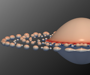
Unlike the prolate fission of droplets in an electric field, the oblate fission of droplets has only gained widespread attention in recent years (Vlahovska Reference Vlahovska2019; Marin Reference Marin2020). Brosseau & Vlahovska (Reference Brosseau and Vlahovska2017) in their groundbreaking experiment discovered that, in a strong electric field, a droplet placed in a medium with higher electric conductivity and permittivity, and lower viscosity, experiences central collapse, leading to an uncontrolled fragmentation. Conversely, when the droplet's viscosity is orders of magnitude smaller than the external medium, it forms a lens-like shape and produces continuously detached liquid rings at the equator. As the liquid rings break, over a hundred satellite droplets are generated in the equatorial plane of the mother droplet, a phenomenon now known as equatorial streaming (Vlahovska Reference Vlahovska2019; Marin Reference Marin2020). In fact, Mohamed et al. (Reference Mohamed, Lopez-Herrera, Herrada, Modesto-Lopez and Gañán-Calvo2016) have found similar phenomena before, where they observed a fragmented liquid ring to form around the droplet perpendicular to the imposed field. This fascinating phenomenon quickly attracted a great deal of interest from researchers due to its ability to produce a large number of size-controllable satellite droplets. Wagoner et al. (Reference Wagoner, Vlahovska, Harris and Basaran2020) solved the steady-state solutions of the LDM equations and obtained the steady shapes of collapsed and lens-shaped droplets, providing a theoretical explanation for the different breakup mechanisms. After that, Firouznia et al. (Reference Firouznia, Miksis, Vlahovska and Saintillan2022) used linear analysis to explore the nonlinear effects generated by the coupling of flowing interfaces and the charge dynamics. More recently, Wagoner et al. (Reference Wagoner, Vlahovska, Harris and Basaran2021) extended their study to transient simulations, indicating that the lens-shaped droplet becomes unstable only with charge relaxation and charge convection. However, research on droplet equatorial streaming is still in its early stage, and there is a lack of a comprehensive understanding of the underlying physics (Wagoner et al. Reference Wagoner, Vlahovska, Harris and Basaran2021). It is also noted that numerical studies replicating the detachment and breakup of liquid rings in equatorial streaming have not been reported.
Currently, simulation methods for multiphase EHD problems mainly include the boundary element method (Betelú et al. Reference Betelú, Fontelos, Kindelán and Vantzos2006; Garzon, Gray & Sethian Reference Garzon, Gray and Sethian2014; Gawande et al. Reference Gawande, Mayya and Thaokar2017, Reference Gawande, Mayya and Thaokar2019), the finite element method (Collins et al. Reference Collins, Jones, Harris and Basaran2008, Reference Collins, Sambath, Harris and Basaran2013; Tian et al. Reference Tian, Wang, Zhou, Xie, Zhu, Xie, Zhu, Chen, Ding and Liao2022; Misra & Gamero-Castaño Reference Misra and Gamero-Castaño2023), EHD–volume of fluid (VOF) method (López-Herrera, Popinet & Herrada Reference López-Herrera, Popinet and Herrada2011; López-Herrera et al. Reference López-Herrera, Gañán-Calvo, Popinet and Herrada2015) and the lattice Boltzmann method (LBM) (Zhang & Kwok Reference Zhang and Kwok2005; Gong, Cheng & Quan Reference Gong, Cheng and Quan2010; Cui, Wang & Liu Reference Cui, Wang and Liu2019; Liu, Chai & Shi Reference Liu, Chai and Shi2019; Luo et al. Reference Luo, Wu, Yi and Tan2020). Collins et al. (Reference Collins, Jones, Harris and Basaran2008, Reference Collins, Sambath, Harris and Basaran2013) successfully employed the finite element method to simulate Coulombic fission for the first time. However, simulating droplet fission in an electric field remains a highly challenging task. For example, boundary element methods often suffer from numerical instability, partly because the droplet's tip becomes singular at the critical moment of fragmentation, where the curvature and the capillary force become infinite. Therefore, existing studies (Gawande et al. Reference Gawande, Mayya and Thaokar2017; Sengupta et al. Reference Sengupta, Walker and Khair2017) typically focus on the behaviours of droplets at the critical moments of fission. The EHD–VOF model has been widely employed in simulating electrohydrodynamic atomization phenomena (López-Herrera et al. Reference López-Herrera, Popinet and Herrada2011; Herrada et al. Reference Herrada, López-Herrera, Gañán-Calvo, Vega, Montanero and Popinet2012). Mohamed et al. (Reference Mohamed, Lopez-Herrera, Herrada, Modesto-Lopez and Gañán-Calvo2016) investigated the fragmentation of suspended droplets above the critical electric field through experiments and numerical simulations, and observed the novel splashing and split-splashing phenomena. They successfully reproduced the droplet splashing using an axisymmetric EHD–VOF model. Recently, López-Herrera, Herrada & Gañán-Calvo (Reference López-Herrera, Herrada and Gañán-Calvo2023) numerically investigated the cone-jet electrosprays of a fully dissociated electrolyte, providing a detailed discussion of the ion concentration of effects.
In existing lattice Boltzmann simulations, charge relaxation and charge convection are usually ignored, with a focus on the situation of infinite electric conductivity (Cui et al. Reference Cui, Wang and Liu2019; Liu et al. Reference Liu, Chai and Shi2019). Also, due to the high computational cost of solving the Poisson equation for the electric field, the majority of simulations are limited to two dimensions (Zhang & Kwok Reference Zhang and Kwok2005; Cui et al. Reference Cui, Wang and Liu2019; Liu et al. Reference Liu, Chai and Shi2019; Luo et al. Reference Luo, Wu, Yi and Tan2020). There is an urgent need to develop a new numerical methodology to simulate the entire process of droplet equatorial streaming. Recently, Luo, Fei & Wang (Reference Luo, Fei and Wang2021) proposed a unified lattice Boltzmann model (ULBM) that integrates commonly used collision operators into a unified framework. The ULBM allows for easy switching between different advanced collision operators while facilitating the extension of LB models for new multiphysics phenomena. Due to its generality and flexibility, the ULBM is well suited for the multiphase flow and coupled multiphysics problems (Wang, Fei & Luo Reference Wang, Fei and Luo2022b; Wang et al. Reference Wang, Yang, Lei, Chen, Wang and Luo2023).
This research aims to numerically investigate the droplet equatorial streaming in an electric field, filling the gap in the simulation of the entire process of this novel phenomenon. In particular, the paper attempts to answer three main questions: (i) whether different breakup mechanisms exist for droplets in a wider range of parameters than in experiments, (ii) how the radius and charge of droplets evolve during equatorial streaming and (iii) what the mechanisms are for the breakup of the liquid ring and the distribution of satellite droplets. To address these questions, a novel multiphase EHD model that considers charge relaxation and charge convection is developed based on the ULBM framework. In order to capture the dynamics of the equatorial streaming process of the entire droplet, fully three-dimensional simulations are conducted. In the following § 2, the governing equations of the problem and the proposed LBM model are introduced. Comprehensive validations and sensitivity analyses of the model are described in § 3. In § 4, we systematically investigate the equatorial flow of liquid droplets, focusing on the breakup outcomes, dynamic evolution and the generation of satellite droplets for a wider range of operation parameters. The conclusions of this study are presented in § 5.
2. Physical and numerical models
2.1. Governing equations for EHD
In this work, the governing equations involving EHD have the following assumptions. First, both the internal medium and the external medium of the droplet are immiscible and incompressible. Second, consistent with experiment (Brosseau & Vlahovska Reference Brosseau and Vlahovska2017), both media are treated as Newtonian fluids with constant physical properties without the influence of gravity. Thirdly, the two-phase EHD is described by the LDM, where the surface charge is treated as the volumetric charge within the interfacial diffusion layer. We assume charge accumulation at the phase interface while no charges exist in the bulk fluid. On the interface, a balance is achieved among surface charges through a competition between the ohmic conduction mechanism, the charge convection mechanism and charge diffusion. To simulate the two-phase flow, the phase-field model is employed, and an improved conservative Allen–Cahn (AC) equation, which was originally proposed in the work of Allen & Cahn (Reference Allen and Cahn1979), is used for interface tracking (Jain Reference Jain2022; Liang et al. Reference Liang, Wang, Wei and Xu2023)
 \begin{equation}\frac{{\partial \phi }}{{\partial t}} + \boldsymbol{\nabla }\boldsymbol{\cdot }(\phi \boldsymbol{u}) = \boldsymbol{\nabla }\boldsymbol{\cdot }{M_\phi }\left( {\boldsymbol{\nabla }\phi - \frac{\boldsymbol{n}}{w}\left[ {1 - {{\tanh }^2}\left( {\frac{{2{\rm T}}}{w}} \right)} \right]} \right),\end{equation}
where  $\phi $ is the phase indicator, for the heavy phase ${\phi _h} = 1.0$ and for the light phase ${\phi _l} = 0$, with ${\phi _0} = ({\phi _h} + {\phi _l})/2 = 0.5$ indicating the position of the interface. Also, n is the unit vector normal to the interface, which is calculated by $\boldsymbol{n} = \boldsymbol{\nabla }\phi /|\boldsymbol{\nabla }\phi |$, ${M_\phi }$ is the mobility and w stands for the interface thickness; $\boldsymbol{u} = [{u_x},{u_y},{u_z}]$ is the fluid velocity. Different from the traditional AC equation, a signed-distance function ${\rm T}\; $ is introduced to avoid any jumps or discontinuities at the interface, where
 \begin{equation}{\rm T} = \frac{w}{4}\ln \left( {\frac{\phi }{{1 - \phi }}} \right).\end{equation}
For the phase-field multiphase model, the conservative AC equation is coupled with incompressible Navier–Stokes (NS) equations, and the continuity and momentum equations for incompressible multiphase flows can be expressed as (Unverdi & Tryggvason Reference Unverdi and Tryggvason1992)
 \begin{equation}\left. {\begin{array}{*{20}{c@{}}} {\boldsymbol{\nabla }\boldsymbol{\cdot }\boldsymbol{u} = 0,}\\ {\dfrac{{\partial (\rho \boldsymbol{u})}}{{\partial t}} + \boldsymbol{\nabla }\boldsymbol{\cdot }(\rho \boldsymbol{uu}) =- \boldsymbol{\nabla }P + \boldsymbol{\nabla }\boldsymbol{\cdot }\left( {\rho \nu (\boldsymbol{\nabla }\boldsymbol{u} + \boldsymbol{\nabla }{\boldsymbol{u}^T}) + \rho \left( {{\nu_b} - \dfrac{2}{3}\nu } \right)(\boldsymbol{\nabla }\boldsymbol{\cdot }\boldsymbol{u})\boldsymbol{I}} \right) + {\boldsymbol{F}_{\boldsymbol{s}}} + {\boldsymbol{F}_{\boldsymbol{e}}},} \end{array}} \right\}\end{equation}
where  $\rho $ indicates the fluid density, $\nu $ is the fluid kinematic viscosity, ${\nu _b}$ stands for the non-hydrodynamic bulk viscosity and P is the pressure; ${\boldsymbol{F}_{\boldsymbol{s}}}$, ${\boldsymbol{F}_{\boldsymbol{e}}}$ are the surface tension and external electric force, respectively,
 \begin{gather}{\boldsymbol{F}_{\boldsymbol{s}}} = {\mu _\phi }\boldsymbol{\nabla }\phi ,\end{gather}
 \begin{gather}{\boldsymbol{F}_{\boldsymbol{e}}} = {\rho _e}E - {\textstyle{1 \over 2}}{\boldsymbol{E}^2}\boldsymbol{\nabla }\varepsilon ,\end{gather}
where  ${\mu _\phi } = 4\beta (\phi - {\phi _l})(\phi - {\phi _h})(\phi - {\phi _0}) - k{\nabla ^2}\phi$ is the chemical potential, and the parameters $\beta = 12\gamma /w$ and $k = 3\gamma w/2$ are related to the interface thickness w and the surface tension $\gamma $. The first term in external electric force ${\boldsymbol{F}_{\boldsymbol{e}}}$ stands for the Coulomb force and the second term represents the dielectric force (Melcher & Taylor Reference Melcher and Taylor1969; Tomar et al. Reference Tomar, Gerlach, Biswas, Alleborn, Sharma, Durst, Welch and Delgado2007).
For the electric field, the governing equation of the field strength follows Gauss's law
 \begin{equation}\boldsymbol{\nabla }\boldsymbol{\cdot }(\varepsilon \boldsymbol{\nabla }\psi ) =- {\rho _e},\end{equation}
where  $\psi $ is the electric potential, and ${\rho _e}$ is the charge density. The electric field strength is given as
 \begin{equation}\boldsymbol{E} =- \boldsymbol{\nabla }\psi .\end{equation}
 In this work, we consider a non-zero bulk charge model. The charge is represented by charge density  ${\rho _e}$, which indicates the concentration of all existing ions (Gañán-Calvo et al. Reference Gañán-Calvo, López-Herrera, Herrada, Ramos and Montanero2018). The evolution of charge density is resolved on the phase diffusion interface. Similar charge density assumptions have been successfully applied in modelling using the EHD–VOF method (López-Herrera et al. Reference López-Herrera, Popinet and Herrada2011). The governing equation for the charge density evolution can be described as the following charge conservation equation (Melcher & Taylor Reference Melcher and Taylor1969; Vlahovska Reference Vlahovska2019):
 \begin{equation}\frac{{\partial {\rho _e}}}{{\partial t}} + \boldsymbol{\nabla }\boldsymbol{\cdot }({\rho _e}\boldsymbol{u}) - \boldsymbol{\nabla }\boldsymbol{\cdot }(\sigma \boldsymbol{\nabla }\psi ) - \alpha {\nabla ^2}{\rho _e} = 0,\end{equation}
where  $\alpha $ is the charge diffusion number and $\sigma $ is the fluid electric conductivity. From the left to the right of the above equation, the first term stands for the charge relaxation, the second term accounts for charge convection, the third term stands for the ohmic conduction and the last term represents the charge diffusion. By introducing characteristic variables ${l_{ch}} = {R_0}$, ${u_{ch}} = {\varepsilon _{ex}}{R_0}E_0^2/{\mu _{ex}}$, ${t_{ch}} = {t_{diff}} = {\mu _{ex}}{R_0}/\gamma $, ${\rho _{ech}} = {\varepsilon _{ex}}{E_0}$, ${\sigma _{ch}} = {\sigma _{ex}}$ and ${\alpha _{ch}} = {\varepsilon _{ex}}R_0^2E_0^2/{\mu _{ex}}$, where the subscript ex refers to the external phase of the droplet, and ${E_0}$ is the electric field strength, the above charge conservation equation can be normalized as
 \begin{equation}\begin{array}{*{20}{c}} {\dfrac{{{t_e}}}{{{t_{diff}}}}\dfrac{{\partial \rho _e^\ast }}{{\partial {t^{\ast }}}} + \dfrac{{{t_e}}}{{{t_{conv}}}}\boldsymbol{\nabla }\boldsymbol{\cdot }(\rho _e^\ast {\boldsymbol{u}^{\ast }}) - \boldsymbol{\nabla }\boldsymbol{\cdot }({\sigma ^\ast }\boldsymbol{\nabla }{\psi ^\ast }) - {\alpha ^\ast }{\nabla ^2}\rho _e^\ast= 0,} \end{array}\end{equation}
where  ${t_e} = {\varepsilon _0}/{\sigma _0}$ stands for the time scale of charge relaxation, ${t_{conv}} = {R_0}/{u_{ch}}$ stands for the time scale of charge convection and ${\alpha ^\ast } = \alpha {\mu _0}/({\varepsilon _0}R_0^2E_0^2)$ is the dimensionless charge diffusion number. Previous studies (Collins et al. Reference Collins, Jones, Harris and Basaran2008, Reference Collins, Sambath, Harris and Basaran2013) indicated that, when ${\alpha ^\ast }$ is less than ${10^{ - 3}}$, charge diffusion has no significant impact on the results; in the following simulations ${\alpha ^\ast }$ is set as ${10^{ - 4}}$.
In most previous simulations of two-phase EHD, the charge density is assumed to be relaxed immediately as the electric field changes, i.e.  ${t_e} \to 0$ (Luo et al. Reference Luo, Wu, Yi and Tan2020). Subsequently, the charge relaxation and the charge convection are ignored. Considering that the charge diffusion is usually negligible compared with the ohmic conduction, the above charge conservation equation can be simplified as $\boldsymbol{\nabla }\boldsymbol{\cdot }(\sigma \boldsymbol{\nabla }\psi ) = 0$. However, Wagoner et al. (Reference Wagoner, Vlahovska, Harris and Basaran2021) theoretically proved that the instability at the equator is only triggered when considering the convection and relaxation of surface charge. Additionally, both Sengupta et al. (Reference Sengupta, Walker and Khair2017) and Wagoner et al. (Reference Wagoner, Vlahovska, Harris and Basaran2020) reported that the jetting of sub-droplets only occurs under finite electric Reynolds numbers $(R{e_e} = {t_e}/{t_{conv}})$. When $R{e_e}$ approaches 0, the droplet exhibits an end-pinching state with conical ends. In this study, we focus on the cone jetting at the equator, which is a problem with $R{e_e}$ in the range of $10\sim {10^5}$, ${t_{diff}}\sim {10^{ - 3}}\ \textrm{s}$ and ${t_{conv}}\sim {10^{ - 4}}\ \textrm{s}$ are of similar magnitude. Therefore, the charge relaxation and charge convection dominate over charge diffusion, and the complete charge conservation equation (2.7) will be solved.
2.2. The ULBM algorithm for the governing equations
In this work, the ULBM framework proposed by Luo et al. (Reference Luo, Fei and Wang2021) is employed to solve the above governing equations. Since the introduction of the ULBM framework, it has been widely applied in simulating various multiphase flows (Yang et al. Reference Yang, Fei, Zhang, Ma, Luo and Shuai2021; Wang et al. Reference Wang, Fei and Luo2022b, Reference Wang, Yang, Lei, Chen, Wang and Luo2023), and phase-change problems (Wang et al. Reference Wang, Fei, Lei, Wang and Luo2022a; Fei et al. Reference Fei, Qin, Zhao, Derome and Carmeliet2023). As a general framework covering different collision models, multiphase flow models and force schemes, it has inherent advantages in simulating multiphase flows coupled with multiple physical fields. The general collision equation for the ULBM model can be expressed as (Luo et al. Reference Luo, Fei and Wang2021; Wang et al. Reference Wang, Fei and Luo2022b)
 \begin{align}
{f_i}(\boldsymbol{x} + {\boldsymbol{e}_i}\Delta t,t +
\Delta t) & = f_i^\mathrm{\ast }(\boldsymbol{x},t) =
{\boldsymbol{\mathsf{M}}^{ - 1}}{\boldsymbol{\mathsf{N}}^{ -
1}}(\boldsymbol{\mathsf{I}} -
\boldsymbol{\mathsf{S}})\boldsymbol{\mathsf{NM}}{f_i}(\boldsymbol{x},t)\notag\\ &
\quad + {\boldsymbol{\mathsf{M}}^{ - 1}}{\boldsymbol{\mathsf{N}}^{ -
1}}\boldsymbol{\mathsf{SNM}}f_i^{eq}(\boldsymbol{x},t) + \Delta
t{\boldsymbol{\mathsf{M}}^{ - 1}}{\boldsymbol{\mathsf{N}}^{ -
1}}(\boldsymbol{\mathsf{I}} - \boldsymbol{\mathsf{S}}/2)\boldsymbol{\mathsf{NM}}{C_i},
\end{align}
\begin{align}
{f_i}(\boldsymbol{x} + {\boldsymbol{e}_i}\Delta t,t +
\Delta t) & = f_i^\mathrm{\ast }(\boldsymbol{x},t) =
{\boldsymbol{\mathsf{M}}^{ - 1}}{\boldsymbol{\mathsf{N}}^{ -
1}}(\boldsymbol{\mathsf{I}} -
\boldsymbol{\mathsf{S}})\boldsymbol{\mathsf{NM}}{f_i}(\boldsymbol{x},t)\notag\\ &
\quad + {\boldsymbol{\mathsf{M}}^{ - 1}}{\boldsymbol{\mathsf{N}}^{ -
1}}\boldsymbol{\mathsf{SNM}}f_i^{eq}(\boldsymbol{x},t) + \Delta
t{\boldsymbol{\mathsf{M}}^{ - 1}}{\boldsymbol{\mathsf{N}}^{ -
1}}(\boldsymbol{\mathsf{I}} - \boldsymbol{\mathsf{S}}/2)\boldsymbol{\mathsf{NM}}{C_i},
\end{align}
where  ${f_i}$ and $f_i^\mathrm{\ast }$ are the pre-collision and post-collision distribution functions, respectively, $f_i^{eq}$ is the equilibrium distribution function and ${C_i}$ is the external forcing term; ${\boldsymbol{e}_i}$ and $\Delta t = 1$ are the discrete velocities and the time step, respectively, and $\boldsymbol{\mathsf{I}}$ stands for the unit matrix.
The generality and universality of the ULBM model are achieved through the implementation of three different matrices: the transformation matrix  $\boldsymbol{\mathsf{M}}$ is used to transform the distribution functions $(\,{f_i})$ to their raw moments $(\boldsymbol{m})$, and the shift matrix $\boldsymbol{\mathsf{N}}$ is used to convert the raw moment collision into the central moment space $(\tilde{\boldsymbol{m}})$, the transformation/shift can be expressed as (Fei & Luo Reference Fei and Luo2017; Fei, Luo & Li Reference Fei, Luo and Li2018)
 \begin{equation}\tilde{\boldsymbol{m}} = \boldsymbol{\mathsf{N}}\boldsymbol{m} = \boldsymbol{\mathsf{NM}}{f_i}.\end{equation}
Finally, the relaxation matrix  $\boldsymbol{\mathsf{S}}$ contains the relaxation parameters which correspond to various models. Through these three matrices, the ULBM model can facilitate the switch between single-relaxation-time collision models (SRT), multiple-relaxation-time collision models (MRT) (Fei et al. Reference Fei, Du, Luo, Succi, Lauricella, Montessori and Wang2019), cascaded lattice Boltzmann models (Fei et al. Reference Fei, Luo and Li2018) and entropy lattice Boltzmann models (Karlin, Bösch & Chikatamarla Reference Karlin, Bösch and Chikatamarla2014; Bösch, Chikatamarla & Karlin Reference Bösch, Chikatamarla and Karlin2015).
In this work, the recently proposed non-orthogonal MRT phase-field ULBM model (ULBM (NMRT) PF) by Wang et al. (Reference Wang, Yang, Lei, Chen, Wang and Luo2023) is adopted to address the aforementioned phase field multiphase model. To capture the realistic dynamic behaviours of droplets in three dimensions, the three-dimensional nineteen-velocity (D3Q19) discrete velocity model is adopted. Two different distribution functions under the raw moment space are introduced to solve the conservation AC equation and the incompressible NS equations
 \begin{gather}\boldsymbol{m}_\phi ^\ast=
\boldsymbol{\mathsf{M}}{f_{\phi ,i}} = (\boldsymbol{\mathsf{I}} -
{\boldsymbol{\mathsf{S}}_\phi }){\boldsymbol{m}_\phi } +
{\boldsymbol{\mathsf{S}}_\phi }\boldsymbol{m}_\phi
^{\boldsymbol{eq}} + \Delta t\left( {\boldsymbol{\mathsf{I}} -
\frac{{{\boldsymbol{\mathsf{S}}_\phi }}}{2}}
\right){\boldsymbol{R}_\phi },\end{gather}
\begin{gather}\boldsymbol{m}_\phi ^\ast=
\boldsymbol{\mathsf{M}}{f_{\phi ,i}} = (\boldsymbol{\mathsf{I}} -
{\boldsymbol{\mathsf{S}}_\phi }){\boldsymbol{m}_\phi } +
{\boldsymbol{\mathsf{S}}_\phi }\boldsymbol{m}_\phi
^{\boldsymbol{eq}} + \Delta t\left( {\boldsymbol{\mathsf{I}} -
\frac{{{\boldsymbol{\mathsf{S}}_\phi }}}{2}}
\right){\boldsymbol{R}_\phi },\end{gather} \begin{gather}\begin{array}{*{20}{c}}
{\boldsymbol{m}_{\boldsymbol{g}}^\mathrm{\ast } =
\boldsymbol{\mathsf{M}}{g_i} = (\boldsymbol{\mathsf{I}} -
{\boldsymbol{\mathsf{S}}_g}){\boldsymbol{m}_g} +
{\boldsymbol{\mathsf{S}}_g}\boldsymbol{m}_g^{eq} + \Delta t\left(
{\boldsymbol{\mathsf{I}} - \dfrac{{{\boldsymbol{\mathsf{S}}_g}}}{2}}
\right){\boldsymbol{R}_g},} \end{array}\end{gather}
\begin{gather}\begin{array}{*{20}{c}}
{\boldsymbol{m}_{\boldsymbol{g}}^\mathrm{\ast } =
\boldsymbol{\mathsf{M}}{g_i} = (\boldsymbol{\mathsf{I}} -
{\boldsymbol{\mathsf{S}}_g}){\boldsymbol{m}_g} +
{\boldsymbol{\mathsf{S}}_g}\boldsymbol{m}_g^{eq} + \Delta t\left(
{\boldsymbol{\mathsf{I}} - \dfrac{{{\boldsymbol{\mathsf{S}}_g}}}{2}}
\right){\boldsymbol{R}_g},} \end{array}\end{gather}
where  $\boldsymbol{m}_\phi ^\mathrm{\ast } = \boldsymbol{\mathsf{M}}{f_{\phi ,i}}$ is for conservation AC equation and $\boldsymbol{m}_{\boldsymbol{g}}^\mathrm{\ast } = \boldsymbol{\mathsf{M}}{g_i}$ is for incompressible NS equations. For the non-orthogonal MRT collision operator, the shift matrix $\boldsymbol{\mathsf{N}} = \boldsymbol{\mathsf{I}}$ and the transformation matrix $\boldsymbol{\mathsf{M}}$ is chosen as the simplified non-orthogonal moment set which was originally proposed by Fei et al. (Reference Fei, Luo and Li2018, Reference Fei, Du, Luo, Succi, Lauricella, Montessori and Wang2019). In the above equation, ${\boldsymbol{m}^{eq}}$ and $\boldsymbol{R}$ are the discrete equilibrium moment set and discrete forcing term in the raw moment space, respectively. The details of the ULBM (NMRT) PF model can be found in the supplementary material S1, available at https://doi.org/10.1017/jfm.2024.441, including explicit expressions of $\boldsymbol{m}_\phi ^{\boldsymbol{eq}}$, ${\boldsymbol{R}_\phi }$, $\boldsymbol{m}_g^{eq}$ and ${\boldsymbol{R}_g}$. As proven in our previous work (Wang et al. Reference Wang, Yang, Lei, Chen, Wang and Luo2023), the above ULBM (NMRT) PF model can accurately recover the target NS equations and interface tracking equation. The ULBM (NMRT) PF has been extensively validated for various complex multiphase flow phenomena such as high density ratio droplet splash and jet spray, demonstrating excellent agreement with experimental results.
Next, the ULBM (NMRT) model is employed to solve the Poisson equation (2.5) for the electric field and the charge conservation equation (2.7) for surface charge. For the charge conservation equation, similar to the AC equation, the D3Q19 non-orthogonal model is utilized. Regarding its collision in the raw moment space, it has
 \begin{align}
\boldsymbol{m}_{{\rho _e}}^\mathrm{\ast } & =
\boldsymbol{\mathsf{M}}f_{{\rho _e},i}^\ast= (\boldsymbol{\mathsf{I}} -
{\boldsymbol{\mathsf{S}}_{{\rho _e}}}){\boldsymbol{m}_{{\rho _e}}} +
{\boldsymbol{\mathsf{S}}_{{\rho _e}}}\boldsymbol{m}_{{\rho _e}}^{eq}
+ \Delta t\left( {\boldsymbol{\mathsf{I}} -
\dfrac{{{\boldsymbol{\mathsf{S}}_{{\rho_e}}}}}{2}}
\right){\boldsymbol{R}_{{\rho _e}}}\notag\\ & \quad + \Delta
t{\boldsymbol{C}_{{\rho _e}}} + 0.5\Delta {t^2}{\partial
_t}({\boldsymbol{C}_{{\rho _e}}}).
\end{align}
\begin{align}
\boldsymbol{m}_{{\rho _e}}^\mathrm{\ast } & =
\boldsymbol{\mathsf{M}}f_{{\rho _e},i}^\ast= (\boldsymbol{\mathsf{I}} -
{\boldsymbol{\mathsf{S}}_{{\rho _e}}}){\boldsymbol{m}_{{\rho _e}}} +
{\boldsymbol{\mathsf{S}}_{{\rho _e}}}\boldsymbol{m}_{{\rho _e}}^{eq}
+ \Delta t\left( {\boldsymbol{\mathsf{I}} -
\dfrac{{{\boldsymbol{\mathsf{S}}_{{\rho_e}}}}}{2}}
\right){\boldsymbol{R}_{{\rho _e}}}\notag\\ & \quad + \Delta
t{\boldsymbol{C}_{{\rho _e}}} + 0.5\Delta {t^2}{\partial
_t}({\boldsymbol{C}_{{\rho _e}}}).
\end{align}For typical convection–diffusion equations such as (2.7), the equilibrium distribution function can be written as (Li et al. Reference Li, Luo, Kang, He, Chen and Liu2016; Lei, Wang & Luo Reference Lei, Wang and Luo2021)
 \begin{equation}\begin{array}{*{20}{c}} {f_{{\rho _e},i}^{eq} = {\rho _e}\omega (|{\boldsymbol{e}_i}{|^2})\left[ {1 + \dfrac{{{\boldsymbol{e}_i}\boldsymbol{\cdot }\boldsymbol{u}}}{{c_s^2}}} \right],} \end{array}\end{equation}
where  $\boldsymbol{u} = [{u_x},{u_y},{u_z}]$ are the velocity components in the x, y and z directions, respectively. The weights are $\omega (0) = 1/3$, $\omega (1) = 1/18$ and $\omega (2) = 1/36$ for the D3Q19 model, and ${C_s} = 1/\sqrt 3 $ stands for the lattice sound speed. The corresponding equilibrium moment set is
 \begin{equation}\boldsymbol{m}_{{\rho _e}}^{eq} = \boldsymbol{\mathsf{M}}f_{{\rho _e},i}^{eq} = {\left[ \begin{array}{@{}l@{}} {\rho_e},{\rho_e}{u_x},{\rho_e}{u_y},{\rho_e}{u_z},0,0,0,{\rho_e},0,0,{\rho_e}{u_x}c_s^2,{\rho_e}{u_x}c_s^2,{\rho_e}{u_y}c_s^2,{\rho_e}{u_z}c_s^2,\\ {\rho_e}{u_y}c_s^2{\rho_e}{u_z}c_s^2,{\rho_e}c_s^4,{\rho_e}c_s^4,{\rho_e}c_s^4 \end{array} \right]^T}.\end{equation}
External force terms are introduced to balance high-order time-related error terms
 \begin{equation}{\boldsymbol{R}_{{\rho _e}}} = {\left[ {\begin{array}{*{20}{@{}c@{}}} {0,{\partial_t}({\rho_e}{u_x}),{\partial_t}({\rho_e}{u_y}),{\partial_t}({\rho_e}{u_z}),0,0,0,0,0,0,{\partial_t}({\rho_e}{u_x})c_s^2,{\partial_t}({\rho_e}{u_x})c_s^2,}\\ {{\partial_t}({\rho_e}{u_y})c_s^2,{\partial_t}({\rho_e}{u_z})c_s^2,{\partial_t}(\phi {\rho_e}{u_y})c_s^2,{\partial_t}(\phi {\rho_e}{u_z})c_s^2,0,0,0} \end{array}} \right]^T}.\end{equation}
The time derivative is calculated by the Eulerian scheme, i.e.
 \begin{equation}\begin{array}{*{20}{c}} {{\partial _t}(\phi \boldsymbol{u}) = \; \dfrac{{{\rho _e}(t)\boldsymbol{u}(t) - {\rho _e}(t - \Delta t)\boldsymbol{u}(t - \Delta t)}}{{\Delta t}}.} \end{array}\end{equation}
 Here,  ${\boldsymbol{C}_{{\rho _e}}}$ is the additional term for ohmic conduction, which is given as
 \begin{align}{\boldsymbol{C}_{{\rho _e}}} = \boldsymbol{\mathsf{M}}\omega (|{\boldsymbol{e}_i}{|^2}){C_{{\rho _e},i}} = {\left[ {\begin{array}{*{20}{@{}c@{}}} {\boldsymbol{\nabla }\boldsymbol{\cdot }(\sigma \boldsymbol{\nabla }\psi ),0,0,0,0,0,0,\boldsymbol{\nabla }\boldsymbol{\cdot }(\sigma \boldsymbol{\nabla }\psi ),0,0,0,0,}\\ {0,0,0,0,\boldsymbol{\nabla }\boldsymbol{\cdot }(\sigma \boldsymbol{\nabla }\psi )c_s^2,\boldsymbol{\nabla }\boldsymbol{\cdot }(\sigma \boldsymbol{\nabla }\psi )c_s^2,\boldsymbol{\nabla }\boldsymbol{\cdot }(\sigma \boldsymbol{\nabla }\psi )c_s^2} \end{array}} \right]^T}.\end{align}
 For the ohmic conduction term, it can be expanded as  $\boldsymbol{\nabla }\boldsymbol{\cdot }(\sigma \boldsymbol{\nabla }\psi ) = \boldsymbol{\nabla }\sigma \boldsymbol{\nabla }\psi + \sigma {\nabla ^2}\psi $. In this paper, for the differential terms associated with solving the electric field, a second-order lattice-based finite difference (FD) scheme is utilized for the solution, where
 \begin{equation}\boldsymbol{\nabla }{\rm I} = \; \sum\limits_i {\frac{{\omega (|{\boldsymbol{e}_i}{|^2}){\rm I}(\boldsymbol{x} + {\boldsymbol{e}_i}){\boldsymbol{e}_i}}}{{c_s^2}}} .\end{equation}
Here,  ${\rm I}$ represents the required differential terms (e.g. $\psi $, $\sigma $). For the Laplacian term of the electric potential ${\nabla ^2}\psi $, through Gauss's law, it is replaced as ${\nabla ^2}\psi =- ({\rho _e} + \boldsymbol{\nabla }\varepsilon \boldsymbol{\nabla }\psi )/\varepsilon $. This transformation is to ensure a coupling between the Poisson equation and the charge conservation equation. Simultaneously, it guarantees the suppression of charge convection only at the phase interface, which can be a great challenge for the LB method since the interface width is typically only 4 to 5 grid points.
Consistent with previous studies (Zhang & Kwok Reference Zhang and Kwok2005; Liu et al. Reference Liu, Chai and Shi2019; Luo et al. Reference Luo, Wu, Yi and Tan2020), a linear interpolation is employed for the dielectric permittivity at the interface, i.e.
 \begin{equation}\varepsilon = {\varepsilon _l} + \frac{{\phi - {\phi _l}}}{{{\phi _h} - {\phi _l}}}({\varepsilon _h} - {\varepsilon _l}),\end{equation}
where  ${\varepsilon _h}$ and ${\varepsilon _l}$ stand for the dielectric permittivity for the heavy phase and light phase, respectively. Due to the linear relationship between $\varepsilon $ and $\phi $, the deviation of $\varepsilon $ can be directly achieved as $\boldsymbol{\nabla }\varepsilon = \boldsymbol{\nabla }\phi ({\varepsilon _h} - {\varepsilon _l})/({\phi _h} - {\phi _l})$ for solving the Poisson equation and the charge conservation equation. On the other hand, the subsequent simulations in this paper will involve very large differences in electric conductivity. Therefore, in order to avoid charge leakage, we innovatively use exponential interpolation to calculate the electric conductivity at the interface, where
 \begin{equation}\ln (\sigma ) = \; \ln ({\sigma _l}) + \frac{{\phi - {\phi _l}}}{{{\phi _h} - {\phi _l}}}(\ln ({\sigma _h}) - \ln ({\sigma _l})).\end{equation}
 Compared with the reciprocal interpolation (see, for example, Tomar et al. Reference Tomar, Gerlach, Biswas, Alleborn, Sharma, Durst, Welch and Delgado2007; Misra & Gamero-Castaño Reference Misra and Gamero-Castaño2023), this exponential interpolation leads to a smoother transition of the dielectric coefficient at the phase interface. Simultaneously, in the following simulations, the viscosity difference between the inner and outer phases can reach magnitudes of  ${10^2}$, with the maximum electric Reynolds number $R{e_e}$ being approximately ${10^4}$. At such a high electric Reynolds number, charge leakage is prone to occur in the lower-viscosity phase. Considering that charge convection only occurs at the phase interface, a smooth limiting function $\boldsymbol{u^{\prime}} = [1 - \tanh (2w(\phi - {\phi _0}))]\boldsymbol{u}$ is introduced for the velocity terms in (2.13) and (2.14) to eliminate charge convection in the bulk phase. In the supplementary material S3, we compared the improvement in charge leakage achieved by the above interfacial scheme with the linear interpolation approach.
The relaxation parameters are determined as  ${s_{{\rho _e},1}} = {s_{{\rho _e},2}} = {s_{{\rho _e},3}} = 1/(\alpha /c_s^2 + 0.5)$. Applying the Chapman–Enskog (CE) analysis in the supplementary material S2, the above ULBM (NMRT) model can recover the target charge conservation equation (2.7) without high-order error terms. Additionally, the remaining relaxation parameters within the relaxation matrix ${\boldsymbol{S}_{{\rho _e}}}$ can be chosen freely, e.g. 1 in our simulations. After the collision in the raw moment space, the distribution function $f_{{\rho _e},i}^\ast $ is reconstructed by $f_{{\rho _e},i}^\ast= {\boldsymbol{\mathsf{M}}^{ - 1}}\boldsymbol{m}_{{\rho _e}}^\mathrm{\ast }$, the charge density can be calculated by
 \begin{equation}{\rho _e} = \sum\limits_i {{f_{{\rho _e},i}}} .\end{equation}
For the Poisson equation of the electric field, the three-dimensional seven-velocity (D3Q7) SRT collision operator is employed for its computation. Due to the necessity of internal iterations at each time step in solving the Poisson equation, the D3Q7 model is sufficient to meet the accuracy requirement. The collision step can be expressed as
 \begin{equation}f_{\psi ,i}^\mathrm{\ast } = {f_{\psi ,i}} - \frac{1}{{{\tau _\psi }}}({\,f_{\psi ,i}} - f_{\psi ,i}^{eq}) + \Delta t^{\prime}{C_{\psi ,i}} + 0.5\Delta {t^{\prime 2}}{\partial _t}({C_{\psi ,i}}),\end{equation}
where  $\Delta t^{\prime} = 1$ is the inner iteration time step, and the equilibrium distribution function is (Chai & Shi Reference Chai and Shi2008)
 \begin{equation}\left. {\begin{array}{*{20}{l@{}}} {f_{\psi ,0}^{eq} = (\tilde{\omega }(|{\boldsymbol{e}_0}{|^2}) - 1)\psi ,}&{i = 0;}\\ {f_{\psi ,i}^{eq} = \tilde{\omega }(|{\boldsymbol{e}_i}{|^2})\psi ,}&{i = 1\sim 6,} \end{array}} \right\}\end{equation}
for the D3Q7 model,  $\tilde{\omega }(0) = 1/4$ and $\tilde{\omega }(1) = 1/8$. Thanks to the generality of the ULBM, the discrete velocities of the D3Q7 model can be obtained directly from the discrete velocity elements of the D3Q19 model (i = 0~6). For the additional term ${C_{\psi ,i}}$ in (2.22), it is given by
 \begin{equation}{C_{\psi ,i}} = \varLambda \frac{{\tilde{\omega }(|{\boldsymbol{e}_i}{|^2})({\rho _e} + \boldsymbol{\nabla }\varepsilon \boldsymbol{\nabla }\psi )}}{\varepsilon },\end{equation}
where  $\varLambda $ is a free relaxation parameter and is set as 0.5 in this work. According to CE analysis, the relaxation time is calculated as ${\tau _\psi } = 1/(\varLambda c_s^2 + 0.5)$, and the electric potential is
 \begin{equation}\psi = \frac{{\sum\limits_{i = 1}^6 {{f_{\psi ,i}}} }}{{1 - \tilde{\omega }(|{\boldsymbol{e}_0}{|^2})}}.\end{equation}
 In this paper, the residual of the electric potential across the whole simulation domain (i.e.  $\epsilon = \sum |\psi (t^{\prime}) - \psi (t^{\prime} - 1)|/\sum |\psi (t^{\prime})|$) is used to determine the convergence of internal iterations at each time step. Specifically, we consider the iterations to be converged when $\epsilon $ is less than ${10^{ - 7}}$ when initializing the electric field, and for each subsequent transient time step, the iteration to have converged when $\epsilon $ is less than ${10^{ - 6}}$.
Figure 1 illustrates the flowchart of the computational process. It is worth noting that the internal iterations for the electric field are computationally expensive. In some previous LB two-phase EHD simulations, the internal iteration step is ignored due to the small deformations of small droplets or adjustable parameters added to expedite the convergence of the Poisson equation (Luo et al. Reference Luo, Wu, Yi and Tan2016, Reference Luo, Wu, Yi and Tan2020). However, given the purpose of this study, focusing on the equatorial streaming of droplets involving significant deformation and fragmentation in an electric field, internal iterations for the electric field are retained. For a typical droplet equatorial streaming simulation, internal iterations for the electric field consume more than 50 % of the computational time.

Figure 1. The flowchart of the computational procedure.
3. Model validations
Before simulating the equatorial streaming of a droplet, we first perform validations and parameter sensitivity tests for the above models. The model is validated by four benchmarks: (i) a single-phase EHD problem; (ii) a multiphase EHD problem with a flat interface; (iii) the deformation of a droplet in an electric field; and (iv) the electrospray of a liquid droplet.
3.1. Single-phase EHD problem
The ULBM model for the charge conservation equation and the Poisson equation for the electric field are first validated by comparing the analytical solution with the numerical solution for charge density relaxation. For a single-phase flow, by neglecting charge convection and charge diffusion, Gauss's law (2.5) and charge conservation equation (2.7) can be simplified to
 \begin{equation}\left. {\begin{array}{*{20}{c@{}}} {{\nabla^2}\psi =- \dfrac{{{\rho_e}}}{\varepsilon },}\\ {\dfrac{{\partial {\rho_e}}}{{\partial t}} = \sigma {\nabla^2}\psi .} \end{array}} \right\}\end{equation}
Therefore, the charge density has the analytical solution
 \begin{equation}{\rho _e} = {\rho _{e,0}}\,{\rm exp} \left( { - \frac{t}{{{t_e}}}} \right).\end{equation}
 The charge relaxation for three different  ${t_e}$ is simulated and the LB simulation results are compared with the analytical solution mentioned above. The results are shown in figure 2(a); qualitatively, our LB simulation results are in perfect agreement with the analytical solution spanning several orders of magnitude of ${t_e}$. The relative errors between the LB simulation results and analytical solutions are plotted in figure 2(b), where the relative error is defined as ${\mathrm{\ \ni }_{{\rho _e}}} = |{\rho _{e,lb}} - {\rho _{e,\; analytical\; }}|/|{\rho _{e,\; analytical\; }}|$. Qualitatively, the maximum relative error between LB simulation results and analytical solutions does not exceed 0.1 %. For all cases, the relative error slightly increases in the later stages, attributed to the fact that the corresponding charge density has relaxed to the order of ${10^{ - 4}}$ of the initial charge at this stage.

Figure 2 (a) Comparison between LB simulation results (symbols) and analytical solutions (lines) for charge density evolution in the bulk phase. (b) Time evolution of relative errors.
3.2. Two-phase EHD problem
Next, a two-phase EHD problem with a simulation domain of size  ${N_x} \times {N_y} \times {N_z} = 5 \times 2 \times 100$ is considered. For this case, we focus on the electric field and charge distribution in the Z direction, so it can be considered as a two-dimensional problem. Therefore, periodic boundary conditions are applied in the x and y directions, respectively, and a zero-gradient boundary condition is applied in the z direction. The lower half $({N_z} < 50)$ of the simulation domain represents the heavy phase, while the upper half $({N_z} \ge 50)$ represents the light phase, with an interface thickness of w = 5. On the top surface of the simulation domain, ${\psi _t} = 10$, and on the bottom surface, ${\psi _b} = 0$. For the light phase, ${\mathrm{\sigma }_l}$ and ${\varepsilon _l}$ are kept as 0.1 and 0.001, respectively. For the heavy phase, ${\sigma _h}$ and ${\varepsilon _h}$ are changed according to the conductivity ratio $R = {\sigma _h}/{\sigma _l}$ and permittivity ratio $S = {\varepsilon _h}/{\varepsilon _l}$, respectively. Ignoring charge convection and charge diffusion, the governing equations of this two-phase EHD problem can be written as
 \begin{equation}\left. {\begin{array}{*{20}{c@{}}} {\boldsymbol{\nabla }\boldsymbol{\cdot }(\varepsilon \boldsymbol{\nabla }\psi ) =- {\rho_e},}\\ {\boldsymbol{\nabla }\boldsymbol{\cdot }(\sigma \boldsymbol{\nabla }\psi ) = 0.} \end{array}} \right\}\end{equation}
 The above equations can be solved by using a second-order FD method. In figure 3, a comparison between our LB simulation results and FD results is presented. The corresponding relative errors are recorded in table 1. Similarly to Fei et al. (Reference Fei, Luo and Li2018), the local relative error between simulation results and FD results for the electric potential is defined as  $\overline {{\ni _\psi}} = \sum |{\psi _{LB}} - {\psi _{FD\; }}|/\sum |{\psi _{FD\; }}|$. As the charge density in the bulk phase is approximately 0, instead of using relative error, the total charge density difference ${\ni _{{\rho _e},t}}\; = |\sum |{\rho _{e,LB}}|- \sum |{\rho _{e,FD}}||/\sum |{\rho _{e,FD}}|$ is used to quantify the error between the LB simulation results and FD results.

Figure 3. Comparison between LB simulation results (hollow symbols) and numerical solutions (lines) for (a)  $\psi $ for cases with different R; (b) ${\rho _e}$ at the phase interface for cases with different R; and (c) for cases with different S.
Table 1. The errors between the LB simulation results and FD results for electric potential and charge density.

Figure 3(a) shows the distribution of electric potential for different values of R ranging from 0.01 to 100. It can be observed that the LB simulation results align closely with the FD solution, with differences observed only near the phase interface. Quantitatively, from table 1, it can be found that the maximum relative errors for the electric potential are less than 3 % for all cases, with the relative errors being slightly increased with R. Figures 3(b) and 3(c) describe the charge density distribution at the phase interface for different R and S cases, respectively. For varying S, the simulation results match closely with the FD results, exhibiting a maximum relative error of 4.23 % at extreme conductivity disparities (i.e. R = 0.01). In the case of different S values, the LB simulation results are almost the same as the FD results, with the maximum relative errors being less than 1 %.
3.3. Deformation of a droplet in an electric field
After validating the accuracy of the electric field and the charge calculations, the simulation is extended to a two-phase EHD problem with fluid flow. Similar to previous studies (Cui et al. Reference Cui, Wang and Liu2019; Liu et al. Reference Liu, Chai and Shi2019; Luo et al. Reference Luo, Wu, Yi and Tan2020), the deformation of a two-dimensional droplet in an electric field is initially simulated. The droplet's initial radius  ${R_0}$ is 30, and the interface thickness w/ ${R_0} = 0.1$. The viscosity and density ratios between the inner and external phases are both set to 1. In this case, the permittivity ratio S is fixed at 3.5, and simulations are conducted for two different values of R = 1.75 and 4.75, with the electric capillary number, $C{a_e} = {\varepsilon _{ex}}{R_0}E_0^2/\gamma $, standing for the ratio of the electric force and surface tension. The initial field strength ${E_0} = ({\psi _t} - {\psi _b})/{N_z}$ is increased from 0.2 to 1.0. In order to consider the effects of charge relaxation and charge convection, a finite $R{e_e} = 1$ is adopted. The droplet's deformation strength $Q = (L - D)/(L + D)$ is recorded, where L and D are the length and diameter of the droplet when it reaches a steady state. The LB simulation results are compared with both the simulations by Liu et al. (Reference Liu, Chai and Shi2019) and the theoretical formula proposed by Feng (Reference Feng2002). In figure 4(a), the results show that, for R = 4.75, the droplet exhibits oblate deformation. Both the simulations by Liu et al. (Reference Liu, Chai and Shi2019) and our current results align well with the theoretical prediction. For R = 1.75, the droplet shows prolate deformation, and our LB results are closer to Feng's (Reference Feng2002) theoretical prediction. It is noticeable that the simulations conducted by Liu et al. (Reference Liu, Chai and Shi2019) overestimate the droplet's deformation strength, possibly due to their neglecting charge relaxation and charge convection effects in their simulations.

Figure 4. (a) Comparison of Q at steady state under different R and  $C{a_e}$ with theoretical solutions and previous simulations. (b) Comparison between current simulation results (bottom) and previous experiment (Grimm & Beauchamp Reference Grimm and Beauchamp2005) (top) for the Rayleigh fission of a methanol droplet in a strong electric field.
We then further extended our simulations to the more challenging three-dimensional two-phase EHD problem, where the LB model for the first time is used to simulate the Coulomb fission of a methanol droplet in a strong electric field. In this simulation, the density ratio of the methanol liquid and ambient gas is  ${\rho _{in}}/{\rho _{ex}} = 1520$, ${\mu _{in}} = 0.032\ \textrm{Pa}\ \textrm{s}$ and viscosity ratio ${\mu _{in}}/{\mu _{ex}} = 320$, surface tension $\gamma = 0.0349\ \textrm{N}\ {\textrm{m}^{-1}}$. The dielectric properties have ${\varepsilon _{in}} = 12.2{\varepsilon _{ex}} = 12.2{\varepsilon _v}$, where ${\varepsilon _v} = 8.854 \times {10^{ - 14}}$ is the vacuum dielectric constant and ${\sigma _{in}} = {10^7}{\sigma _{ex}} = 0.1\ \textrm{S}\ {\textrm{m}^{ - 1}}$. The initial radius of the droplet is ${R_0} = 10\,\mathrm{\mu }\textrm{m}$. Similar to experiment (Grimm & Beauchamp Reference Grimm and Beauchamp2005), the strength of the external electric field is set to a value greater than ${E_c}$, e.g. ${E_0} = ({\psi _t} - {\psi _b})/\; {N_z} = 1.17{E_c}$ for the target experiment, where the Taylor limit field strength is calculated as ${E_c} = \sqrt {4\gamma /({\sigma _{ex}}{R_0})} $. For our current simulation, the mesh resolution is $\textrm{d}\kern0.7pt x = {R_0}/60$ and time step is $\textrm{d}t = 7.5 \times {10^{ - 6}}\ \textrm{s}$. The simulation domain is a ${N_x} \times {N_y} \times {N_z} = 5{R_0} \times 5{R_0} \times 16{R_0}$ box. The comparison between simulation and experimental results (Grimm & Beauchamp Reference Grimm and Beauchamp2005) is shown in figure 4(b), where an excellent agreement is found between our simulation and the experimental snapshots. Notably, the liquid filament at the tip of the droplet is successfully captured, with a radius approximately one order of magnitude smaller than ${R_0}$ as observed in experiments (Duft et al. Reference Duft, Achtzehn, Müller, Huber and Leisner2003; Grimm & Beauchamp Reference Grimm and Beauchamp2005; Cai et al. Reference Cai, Sun, Wang, Yang, Li and Yu2021).
At the end of this section, the mesh sensitivity analysis and charge conservation validation are conducted. In this test, the deformation of a methanol droplet at two different electric field intensities ( ${E_0} = 0.25{E_c}$ and ${E_0} = 0.8{E_c}$) is simulated. The physical properties of the methanol droplet are consistent with the simulation parameters in figure 4(b), with the electrical conductivity ratios ${\sigma _{in}}/{\sigma _{ex}}$ equals ${10^7}$. The grid resolution ${R_0}/\textrm{d}\kern0.7pt x$ is increased from 30 to 60, with corresponding $\textrm{d}\kern0.7pt x$ ranges from $0.15$ to $0.3\,\mathrm{\mu }\textrm{m}$ in physical units. The evolution of the aspect ratio (L/D) during the process is depicted in figure 5(a). The results indicate that, for the case with lower electric field intensities $({E_0} = 0.25{E_c})$, when ${R_0}/\textrm{d}\kern0.7pt x$ is greater than 30, the grid resolution has little impact on the simulation results. For the case with higher electric field intensities $({E_0} = 0.8{E_c})$, only minor differences were observed for the lowest resolution $({R_0}/\textrm{d}\kern0.7pt x = 30)$ in the final stage (as illustrated in the inset), during which the tip of the droplet begins to develop a liquid filament. The time evolution of the error in the total charge of the droplet during its deformation process is also recorded, where the error is calculated as ${\epsilon _{{\rho _e}}} = \sum {\rho _e}/\sum |{\rho _e}|\times 100\,\%$. Ideally, $\sum {\rho _e}$ should be kept as 0 when the conservation of charge is fully satisfied. As shown in figure 5(b), the charge error for the proposed LB model in this study is below 0.8 %. For denser grids (i.e. ${R_0}/\textrm{d}\kern0.7pt x = 60$), this error is reduced to less than 0.1 %.

Figure 5. Time evolution of (a) aspect ratio of the droplet and (b) charge error under different grid resolutions.
3.4. Simulation of droplet electrospray
In this section, we simulate the electrospray of a suspended liquid droplet in an electric field and compare the ejected diameter with the scaling laws proposed by Gañán-Calvo et al. (Reference Gañán-Calvo, López-Herrera, Rebollo-Muñoz and Montanero2016). Table 2 summarizes the properties of the liquid droplets used in our simulations, where the governing dimensionless number  ${\varGamma _u}$ is ${\varGamma _u} = \delta _u^{5/3}{({\varepsilon _{in}}/{\varepsilon _{ex}})^{5/12}}$, and the parameter ${\delta _u}$ is given as ${\delta _u} = {[({\gamma ^2}{\rho _{in}}{\varepsilon _{ex}})/(\mu _{in}^3{\sigma _{in}})]^{1/3}}$ (Gañán-Calvo Reference Gañán-Calvo1999). Six different cases with a wide range of ${\varGamma _u}$ are simulated. Figure 6(a) illustrates the qualitative evolution of liquid droplets under three different values of ${\varGamma _u}$. It can be observed that, similar to the results obtained from experiments and simulations (Gañán-Calvo et al. Reference Gañán-Calvo, López-Herrera, Rebollo-Muñoz and Montanero2016), the suspended droplets are elongated under the influence of electric field forces, forming a liquid jet and undergoing electrospraying. Moreover, consistent with the qualitative findings from experiments (Gañán-Calvo et al. Reference Gañán-Calvo, López-Herrera, Rebollo-Muñoz and Montanero2016), the diameter of the ejected droplet ${d_l}$ from the jetting tip is increased with ${\varGamma _u}$. Furthermore, the ejection time and the length of the jet are also increased with ${\varGamma _u}$ due to a slower charge relaxation.

Figure 6 (a) Evolution of droplet profiles under different  ${\varGamma _u}$. (b) Quantitative comparison of ejected droplet diameters with experimental results and linear fitting equation.
Table 2. Liquid properties of the electrospray simulation.

Figure 6(b) presents a quantitative comparison between our LB simulation results of  ${d_l}$ and experimental results (Gañán-Calvo et al. Reference Gañán-Calvo, López-Herrera, Rebollo-Muñoz and Montanero2016). The dashed line in the figure represents the linear fitted function ${d_l} = 0.6{\varGamma _u}(\mu _{in}^2/\gamma )$ (Gañán-Calvo et al. Reference Gañán-Calvo, López-Herrera, Rebollo-Muñoz and Montanero2016). It can be observed that our simulation results are in line with the experimental data and the linear fitted function across a wide range of ${\varGamma _u}$. Besides, it is found that our LB simulation results exhibit good agreement with the simulation results and experimental data achieved by Gañán-Calvo et al. (Reference Gañán-Calvo, López-Herrera, Rebollo-Muñoz and Montanero2016). This is because both our EHD–LB model and their EHD–VOF model consider the effects of electric charge transport at the interface. On the other hand, the charge convection is considered in our simulations while it is ignored in the EHD–VOF model. Compared with the experimental results, our simulations slightly overestimated the size of ${d_l}$. In conclusion, the good agreement between our simulation results and experimental/theoretical results in the present validation test provides evidence that our proposed model can accurately simulate complex EHD phenomena.
4. Study of droplet equatorial streaming in an electric field
In this chapter, the validated LB model is employed to simulate the equatorial streaming of a droplet in an electric field. Firstly, it introduces the numerical set-up and simulation parameters. Then, it presents the morphologies of droplet equatorial streaming under different simulation conditions. Subsequently, a detailed analysis of the dynamic evolution of the droplet before its first breakup is conducted. Finally, the mechanisms of droplet breakup during equatorial streaming are discussed.
4.1. Problem description and numerical set-up
Figure 7 shows the simulation domain in Cartesian coordinates, with a droplet placed at the centre of a rectangular box. The initial radius of the liquid droplet is  ${R_0}$. The dimensions of the simulation domain are set to a length (L) and width (W) of $9{R_0}$, with a height $({L_z})$ of $5{R_0}$. The top and bottom walls are designated as no-slip boundaries and are assigned constant voltages. The voltage on the top surface is ${\psi _{max}}$, and on the bottom surface is ${\psi _{min}}$. The four lateral walls are set as periodic boundaries. $\gamma $, ${\rho _i}$, ${\mu _i}$, ${\varepsilon _i}$ and ${\sigma _i}$ represent surface tension, density, viscosity, dielectric permittivity and electrical conductivity, respectively, where the subscript i is used to specify the external phase $(ex)$ or the internal phase $(in)$.

Figure 7. Schematic of the simulation domain.
To reproduce the droplet equatorial streaming in an external electric field, following the experiment of Brosseau & Vlahovska (Reference Brosseau and Vlahovska2017), the internal phase is set as low-viscosity silicone oil (SO) with low electrical conductivity ( ${\rho _{in}} = 910\ \textrm{kg}\ {\textrm{m}^{ - 3}}$, ${\mu _{in}} = 0.0048\ \textrm{Pa}\ \textrm{s}$, ${\varepsilon _{in}} = 3.2{\varepsilon _v}$, ${\sigma _{in}} = 2 \times {10^{ - 12}}\ \textrm{S}\ {\textrm{m}^{ - 1}}$), while the external phase is set as high-viscosity castor oil with high electrical conductivity ( ${\rho _{ex}} = 900\ \textrm{kg}\ {\textrm{m}^{ - 3}}$, ${\mu _{ex}} = 0.48\ \textrm{Pa}\ \textrm{s}$, ${\varepsilon _{ex}} = 4.59{\varepsilon _v}$ and ${\sigma _{ex}}$ is varied correspondingly with the conductivity ratio $R = \; {\sigma _{in}}/{\sigma _{ex}}$). The surface tension and radius of the droplet are chosen as the same as the experiment, i.e. $\gamma = 0.0041\ \textrm{N}\ {\textrm{m}^{ - 1}}$ and ${R_0} = 1\ \textrm{mm}$. The field strength of the external electric field is determined by the voltage contrast of the bottom wall and top wall, where ${E_0} = ({\psi _{max}} - {\psi _{min}})/{L_z}$. It is worth noting that the conversion between lattice units and physical units requires selection of appropriate reference length and time scales. In the following simulations, the reference length $\textrm{d}\kern0.7pt x = {R_0}/50 = 20\,\mathrm{\mu }\textrm{m}$ and reference time $\textrm{d}t = 7.5 \times {10^{ - 6}}\ \textrm{s}$ were employed. It should also be noted that, for the current set-up, the total grid number of the simulation domain exceeds 50 million. Our code is parallelized by using MPI, and for a typical case (modelling the dynamic behaviours of the droplet for 1.1 s), the computational cost is approximately 4000 CPU running over 10 hours. All simulations are conducted on the United Kingdom national supercomputer Archer2.
This study aims to obtain a further understanding of droplet equatorial streaming. To this end, two governing parameters of the process are focused on: the electric field strength  $({E_0})$ and the conductivity contrast (1/R). In the existing studies for droplet equatorial streaming (Brosseau & Vlahovska Reference Brosseau and Vlahovska2017; Wagoner et al. Reference Wagoner, Vlahovska, Harris and Basaran2020, Reference Wagoner, Vlahovska, Harris and Basaran2021), details of droplet evolution at higher conductivity contrasts (i.e. $1/R > 2000$) remain unknown. Regarding the influence of electric field strength, it has not been systematically explored in previous experimental and simulation studies. For a droplet undergoing Coulomb fission, a necessary condition is that ${E_0} > {E_c} = 6.35\ \textrm{KV}\ \textrm{c}{\textrm{m}^{ - 1}}$ (Gawande et al. Reference Gawande, Mayya and Thaokar2017; Misra & Gamero-Castaño Reference Misra and Gamero-Castaño2023). Besides, for the droplet equatorial streaming, the electrical conductivity contrasts have $1/R \gg 1$ (Wagoner et al. Reference Wagoner, Vlahovska, Harris and Basaran2020, Reference Wagoner, Vlahovska, Harris and Basaran2021). Subsequently, for the following simulation, we change 1/R from 800 to 10 000, and ${E_0}$ is varied from $0.75{E_c}$ to $2.0{E_c}$, with the corresponding electric capillary number $C{a_e}$ ranging from 2.2 to 16.
4.2. Morphologies of droplet equatorial streaming
Figure 8(a) illustrates a typical process of a droplet equatorial streaming in an electric field, where  ${E_0} = 1.05{E_c}$ and $1/R = 2000$. The droplet is observed to gradually flatten under the effects of the electric field. A liquid lamella becomes noticeable at the equator of the mother droplet, because of the squeezing effect. As the droplet continues to deform, the liquid lamella forms a liquid ring and detaches from the equator. The detached ring continues to expand while an instability wave develops over it, eventually breaking into dispersed satellite droplets. During the process, new liquid rings continue to form from the equator of the mother droplet, undergoing expansion and breakage, thus constituting the equatorial streaming of the droplet. Figure 8(b) shows a qualitative comparison of the simulation snapshot with the experimental snapshot (Brosseau & Vlahovska Reference Brosseau and Vlahovska2017) for drop equatorial streaming. As can be seen, our simulation successfully reproduces the equatorial streaming phenomenon that when a droplet is subjected to an electric field, concentric fluid rings around the droplet are generated from the equator of the droplet, which finally break up to form hundreds of satellite droplets.

Figure 8. (a) Transient evolution of droplet equatorial streaming. (b) Experimental (Brosseau & Vlahovska Reference Brosseau and Vlahovska2017) (left snapshot) and simulation results (right snapshot) of the equatorial streaming for a droplet; simulation snapshot with the droplet surface coloured by charge density.
Subsequently, we conducted simulations over a wider range of operation parameters, revealing two distinct break mechanisms behind the droplet equatorial streaming. Under conditions similar to the experimental conditions (Brosseau & Vlahovska Reference Brosseau and Vlahovska2017), i.e. lower  ${E_0}$ and smaller 1/R, the droplets displayed a liquid ring equatorial streaming process which is the same as the experimental results. However, for high ${E_0}$ and large 1/R, the droplets exhibit a novel fingering equatorial streaming process. Figure 9 qualitatively illustrates the different break mechanisms of equatorial streaming under various conditions. Results with a blue background represent ring equatorial streaming of the droplets, while those with a red background depict fingering equatorial streaming. Unlike the ring equatorial streaming described in figure 8(a), for fingering equatorial streaming, multiple liquid fingers are generated at the equator of the mother droplet. Subsequent satellite droplets can be observed continuously detaching from these liquid fingering tips at the equator, as opposed to those being generated due to the continuous breakup of liquid rings. Supplementary movie 1 and movie 2 show the evolution of ring equatorial streaming (1/R = 1500, ${E_0} = 1.05{E_c}$) and the fingering equatorial streaming (1/R = 2000, ${E_0} = 1.50{E_c}$), respectively. Additionally, it is evident that the number and size of satellite droplets vary in mechanisms, which will be analysed quantitively in the following text.

Figure 9. Snapshots of droplet equatorial streaming under different simulation parameters. Images in blue background represent ring equatorial streaming, and those in red background indicate fingering equatorial streaming.
In figure 10, temporal evolutions of the generation and the breaking processes of the liquid rings/fingers at the equatorial plane of the droplet are presented, where the droplet surface is coloured by the magnitude of the external electric force. In the figure, the first three columns of contours on the left represent the first, second and third detachments of liquid rings, respectively. It can be found that the external electric field force is maximum near the equator of the mother droplet, where the squeezing of the electric field force leads to the elongation and fragmentation of the liquid lamella at the equator. For the cases of  ${E_0} = 1.05{E_c}$, it is observed that a larger 1/R (i.e. 1/R = 2000) resulted in a quicker detachment and breakup of the liquid rings. Compared with the case with a smaller 1/R (1/R = 800), the satellite droplets generated were smaller in size but more plentiful in number. The breakup of the liquid rings via a classical capillary instability (which is also known as Rayleigh Plateau instability) (Burton & Taborek Reference Burton and Taborek2011; Gawande et al. Reference Gawande, Mayya and Thaokar2019), involves the continuous formation of necking and expansion along the circular direction. The experimental snapshot (grey inset) also confirmed this phenomenon. For the case of fingering equatorial streaming ( ${E_0} = 1.50{E_c}$ and R = 1/2000), its initial state is similar to ring equatorial streaming, where 2–3 liquid rings detach from the mother droplet and break into satellite droplets. In this case, it is observed that the first liquid ring is accompanied by a smaller daughter liquid ring, which is consistent with the experimental findings (Brosseau & Vlahovska Reference Brosseau and Vlahovska2017). Then, as the last ring detaches (t = 0.236 s), unstable liquid fingers develop at the edge of the mother droplet. These unstable liquid fingers are excited by instability waves in continuously detaching liquid rings. It can be evidenced that, with the detachment of the last ring, liquid fingers immediately form, and there is continuous contraction and expansion on the last detached ring (at t = 0.281 s). After the appearance of the liquid fingers, all subsequent satellite droplets are directly generated from the tip of the fingers, demonstrating an unstable mechanism distinct from the ring equatorial streaming. Regarding the diameter of the detached liquid rings, we observe that, in cases with relatively low electric field strength (i.e. ${E_0} = 1.05{E_c}$), the diameters of the first three detached liquid rings are similar, with a diameter of approximately ${d_r}/{d_0}\sim 0.04$. However, for cases with higher electric field strength (i.e. ${E_0} = 1.5{E_c}$), the detachment of the first larger liquid ring ${d_r}/{d_0}\sim 0.06$ is immediately followed by the detachment of a smaller ring ${d_r}/{d_0}\sim 0.02$. Such occurrences of smaller sub-liquid ring detachment have also been observed in experiments (Brosseau & Vlahovska Reference Brosseau and Vlahovska2017). In the following § 4.3, we provide a detailed discussion and analysis of the sizes of detached liquid rings and satellite droplets.

Figure 10. Dynamic evolution of localized magnification of droplet ring equatorial streaming (blue background) and fingering equatorial streaming (red background). The droplet surface is coloured by the electric field force magnitude. The inset figure (grey) represents the experiment (Brosseau & Vlahovska Reference Brosseau and Vlahovska2017) snapshot of droplet equatorial streaming.
As indicated in figures 8 and 10, compared with experimental results, the diameter of the liquid ring  $({d_r})$ is wider in our simulation results, and the gaps between the liquid rings are large (e.g. when ${\mu _{in}}/{\mu _{ex}} = 100$, ${d_r}/{d_0}\sim 0.01$ for experiment, ${d_r}/{d_0}\sim 0.04$ for our simulations). Several reasons may account for these discrepancies: (i) our simulation conditions may not perfectly match the experimental conditions, as the accurate value for 1/R was not provided in the original experimental results. (ii) In our simulations, the conductivity and dielectric permittivity at the interface are characterized by using log interpolation and linear interpolation. In reality, the distribution of electrical properties between the different phases is more complex. (iii) Limited by the computational resources, the interface thickness is set as $w/{d_0} = 0.05$. This implies that the interface width is still of the order of micrometres. For real-world scenarios, the interface thickness is often in the nanometre range. Despite there being some quantitative differences between the simulation and experimental results, it is important to note that the model proposed in this paper qualitatively replicates the equatorial streaming process of a liquid droplet. Specifically, the model accurately captures, for the first time, the continuous detachment of the liquid rings from the equator and the subsequent splitting of the liquid rings into several hundred satellite droplets. Also, thanks to the quantitative results provided by numerical simulations, in the following study we reveal the power-law relation for the charge evolution during droplet equatorial streaming, propose a theoretical model for the evolution of the droplet radius and height and quantitatively investigate the breakup mechanism of the droplet. Moreover, by changing the operation conditions, our simulations revealed a new fingering equatorial streaming mechanism. These results are essential for studying the underlying physical mechanisms of droplet equatorial streaming.
To gain a better understanding of why different values of  ${E_0}$ and 1/R lead to distinct instability mechanisms, we quantitatively analyse the profiles (first row), charge density ( ${\bar{\rho }_e}$, second row) and lateral external electric force ( ${\boldsymbol{F}_{e\_x}}$, third row, the ‘+’ and ‘−’ symbols represent the directions of liquid droplet expansion and contraction, respectively) near the liquid lamella at the equator before its first breakup under various 1/R (figure 11a) and ${E_0}$ (figure 11b). The droplet profile is divided into three different regions along the expansion direction (X-axis) based on the morphologies. Region I, situated near the mother droplet, exhibited similar morphologies for various 1/R, and with nearly uniform ${\boldsymbol{F}_{e\_x}}$, which is due to the fact that the mother droplet is mainly squeezed by the longitudinal external electric field force. For cases with different ${E_0}$, this region also displayed consistent profiles, similar ${\bar{\rho }_e}$ and ${\boldsymbol{F}_{e\_x}}$. It is noteworthy that in cases with higher ${E_0}$, ${\bar{\rho }_e}$ in this region is larger, which confirms Gauss's law (Melcher & Taylor Reference Melcher and Taylor1969).

Figure 11. For cases with different (a) 1/R and (b)  ${E_0}$, at the critical moment before the first liquid ring detachment from the droplet, the profiles of the liquid lamella near the droplet equator (first row), the corresponding distribution of charge density (second row) and the corresponding electric field force in the direction of droplet expansion (third row).
As for region II, corresponding to the neck position of the liquid lamella, the maximum value of  ${\bar{\rho }_e}$ on the droplet's surface is observed at this location. This finding is distinct from the previous extensive modelling of perfectly dielectric droplets, where the maximum value of ${\bar{\rho }_e}$ appears at the droplet conical tips (Gawande et al. Reference Gawande, Mayya and Thaokar2017, Reference Gawande, Mayya and Thaokar2019; Sengupta et al. Reference Sengupta, Walker and Khair2017). For equatorial streaming, it occurs at the neck of the equatorial liquid lamella, which is compatible with the theoretical findings for the finite conductivity model (Gawande et al. Reference Gawande, Mayya and Thaokar2019; Misra & Gamero-Castaño Reference Misra and Gamero-Castaño2023). Furthermore, it can be found that the maximum charge increased with 1/R and ${E_0}$, which also aligns with Gauss's law. Regarding the magnitude of ${\boldsymbol{F}_{e\_x}}$, it initially increased in the direction of retraction (−x) and then increased in the direction of expansion (+x), which manifested as a stretching force (as marked in figure 11). It is this stretching force and its competition with surface tension that leads to the contraction of the liquid lamella in the longitudinal direction, forming the lamella neck. Quantitatively, it can be observed the stretching force increased with 1/R and ${E_0}$. The qualitative results in figure 11 indicate that the appearance of the liquid fingers is caused by the destabilization of the liquid rings at the equator, before they are detached from the mother droplet. From the quantitative results in figure 11, it is proved that higher ${E_0}$ and 1/R result in greater stretching forces, implying a faster liquid ring departure velocity. Previous studies have found that the instability wave on the liquid ring is positively correlated with the expansion velocity of the liquid ring (Stone Reference Stone1994; Zhao & Tao Reference Zhao and Tao2016). And in such cases, the breakup points are closer to the mother droplet. This explains why the phenomenon of equatorial streaming is observed with higher ${E_0}$ and 1/R.
Region III represents the tip region of the liquid lamella, where  ${\bar{\rho }_e}$ rapidly decreases from the maximum value to zero at the equatorial tip (point B in figure 8). The value of ${\boldsymbol{F}_{e\_x}}$ in the droplet's expansion direction initially decreases to zero and then increases in the direction of retraction. Considering that ${\bar{\rho }_e}$ is zero at this point, the electric field force here is solely contributed by the dielectric force. Therefore, from figure 11, it can be observed that ${\boldsymbol{F}_{e\_x}}$ at the equatorial tip increases with 1/R and is almost independent of ${E_0}$. This finding is consistent with (2.7). For the maximum spreading diameter of the droplet before breakup, it is found that it decreased with increasing 1/R, whereas it increased with increasing ${E_0}$.
In this subsection, the equatorial streaming of a liquid droplet under different 1/R and  ${E_0}$ is qualitatively demonstrated, revealing two distinct morphologies: ring equatorial streaming and fingering equatorial streaming. A qualitative overview of the detachment of the liquid lamella at the equator, the formation of the liquid rings/liquid fingers and the generation of satellite droplets is provided. Subsequently, quantitative analysis of the charge distribution and external electric force on the liquid lamella are employed to explain the generation of fingering equatorial streaming. The following subsection will focus on the dynamic behaviours of the droplet before it breaks, with emphasis on quantitatively studying critical parameters such as the droplet's total charge, spreading diameter and droplet breakup time.
4.3. Dynamic behaviours of the droplet
In the study of the EDH phenomenon, a critical point is understanding the behaviours of the charge density (Fernández de la Mora Reference Fernández de la Mora2007; Vlahovska Reference Vlahovska2019), especially its dynamic evolution over time and the charge carried by satellite droplets. This is of paramount importance for applications such as mass spectrometry analysis, separations, powder synthesis and others (Fenn et al. Reference Fenn, Mann, Meng, Wong and Whitehouse1989; Ptasinski & Kerkhof Reference Ptasinski and Kerkhof1992; Harris, Scott & Byers Reference Harris, Scott and Byers1993). After applying an electric field, the charge equilibrium is disrupted. Positive and negative charges at the phase interface are driven towards the positive and negative ends closer to the electrodes under the influence of Coulomb forces (Fernández de la Mora Reference Fernández de la Mora2007; Luo et al. Reference Luo, Wu, Yi and Tan2020). In all cases, due to charge conservation, the total charge always equals 0. Therefore,  ${Q_e} = \sum |{\rho _e}|$ is used to represent the total charge carried by the droplet. To explore the mechanism of charge evolution under different simulation parameters, the time is normalized by introducing a charge relaxation time that takes into account differences in electrical conductivity and dielectric coefficients (i.e. $t_e^\sim= {t_e}(2 + S)/(2 + R)$) (Brosseau & Vlahovska Reference Brosseau and Vlahovska2017). Regarding ${Q_e}$, it is normalized by using $Ca_e^{0.5}{q_c}$, where ${q_c}$ is the Rayleigh charge limitation ${q_c} = 8{\rm \pi}\sqrt {\gamma {\varepsilon _{ex}}R_0^3} $.
The evolutions of the total charge of the droplet before the first ring detaching for different 1/R and  ${E_0}$ cases are plotted in figure 12 with a logarithmic scale. It can be observed that, for all cases when $t/t_e^\sim < 1$ (blue background), the evolution of the total charge follows a power-law increase, with its evolution being fitted as
 \begin{equation}\frac{{{Q_e}}}{{Ca_e^{0.5}{q_c}}} = 0.25\; {\left( {\frac{t}{{t_e^\sim }}} \right)^{0.95}}.\end{equation}
This result confirms the findings of Sengupta et al. (Reference Sengupta, Walker and Khair2017), who also found a power-law increase for the surface charge. The consistency exhibited by the total charge in this region is due to the fact that the evolution of the charge is dominated by the charge relaxation. Dividing time and total charge by  $t_e^\sim $ and $Ca_e^{0.5}{q_c}$, the influence of the charge relaxation can be normalized appropriately. Outside this region, the charge evolution varies from case to case. Specifically, the total charge increases faster under conditions of higher ${E_0}$ and lower 1/R. As pointed out by Sengupta et al. (Reference Sengupta, Walker and Khair2017), within this region, the influence of charge convection cannot be neglected, particularly for cases with larger Reynolds numbers $(R{e_e})$. Considering $R{e_e}$ increases with ${E_0}$ but decreases with 1/R, our simulation results corroborate with the prediction from Sengupta et al. (Reference Sengupta, Walker and Khair2017).

Figure 12. Evolution of the total charge carried by the droplet before the first liquid ring detachment, under different simulation conditions. The region dominated by charge relaxation is indicated by the blue background.
Next, the evolution of the droplet's height (H) and radius (R) before the first detachment of the liquid ring is investigated. Figures 13(a) and 13(b) indicate the time evolution of the droplet deformation magnitude in radius  $(\Delta {r^\ast } = (R(t) - {R_0})/{R_0})$ and height $\mathrm{(\Delta }{h^\ast}=({R_0} - H(t))/{R_0})$ under various 1/R and ${E_0}$, respectively. In the figure, $\mathrm{\Delta }{r^\ast }$ and $\mathrm{\Delta }{h^\ast }$ are generalized by using $C{a_e}$ and time t is normalized by capillary time ${t_c} = {(R_0^3{\rho _{ex}}/\gamma )^{0.5}}$. The inset figure in figure 13(a) represents the initial state of droplet motion, it can be found that the droplet remains stationary for a very short period $({t_0},{t_0} \ll {t_c})$ after applying the electric field. This very short stationary time is directly proportional to the charge relaxation time. Considering the charge relaxation time decreases when 1/R is increased, $t_e^\sim (10\;000)$ is used as a reference value (standing for the $t_e^\sim $ when 1/R = 10 000), the dynamic stationary time is given as ${t_0} = 0.5(t_e^\sim (1/R) - t_e^\sim (10\;000))$.

Figure 13. Under different simulation conditions, the time evolution of deformation magnitude in (a) height and (b) radius of the droplet before the first liquid ring detachment.
In figure 13, all the normalized results can be collapsed into one line. In this work, a new theoretical model is proposed to describe the transient evolution of the droplet height and radius. First, let us consider the transient evolution of the droplet in the direction of the electric field. To facilitate the analysis, we only consider forces on the symmetry plane of the droplet, i.e. on the x–z plane. When subjected to an electric field, the poles of the droplet (point A in figure 8) are subjected to a capillary force  $({F_c}\sim 2\gamma /H)$, viscous force $({F_v}\; \sim \; {\mu _0}/{R_0}\Delta H^{\prime})$ and electric field force $({F_e}\sim {\varepsilon _0}E_0^2)$. According to Newton's second law, we can determine
 \begin{equation}{m^\ast }\frac{{{d^2}(\Delta {h^\ast }{R_0})}}{{\textrm{d}{t^2}}}\sim \; {\varepsilon _0}E_0^2 - \frac{{2\gamma }}{{{R_0}(1 - \Delta {h^\ast })}} - \frac{{{\mu _{ex}}}}{{{R_0}}} \times \frac{{\textrm{d}(\Delta {h^\ast }{R_0})}}{{\textrm{d}t}},\end{equation}
where  ${m^\ast }$ is the effective mass, with a dimension of $\textrm{kg}\ {\textrm{m}^{ - 2}}\sim {\rho _{ex}}{R_0}$ in this two-dimensional analysis. By non-dimensionalizing the above equations with ${t^\ast } = (t - {t_0})/{t_c}$
 \begin{equation}\frac{{{d^2}\Delta {h^\ast }}}{{\textrm{d}{t^{{\ast} 2}}}}\sim \; \; C{a_e} - \frac{2}{{(1 - \Delta {h^\ast })}} - Oh\frac{{\textrm{d}\Delta {h^\ast }}}{{\textrm{d}{t^\ast }}}.\end{equation}
The Ohnesorge number  $Oh = {\mu _{ex}}/\sqrt {2\gamma {\rho _{ex}}{R_0}} = 7.9$ is kept consistent for all cases. This non-dimensional number measures the ratio of viscous forces to surface tension and inertial forces. For the case of $Oh > 1$, the viscous force is dominant. Considering the surface tension of the simulated SO droplet is relatively small, for the initial stage of droplet motion, deformation is primarily governed by the competition between electric field forces and viscous forces. Therefore, we neglect the term related to surface tension. By incorporating the initial conditions $\textrm{d}\Delta {h^\ast }/\textrm{d}{t^\ast } = 0$ and $\mathrm{\Delta }{h^\ast } = 0$ when $\; {t^\ast } = 0$, the above differential equation has the general solution
 \begin{equation}\Delta {h^\ast } = \alpha \left\{ {\frac{{\; C{a_e}}}{{Oh}}(t - {t_0})/{t_c} + \frac{{\; C{a_e}}}{{{{(Oh)}^2}}}({\textrm{e}^{ - Oh(t - {t_0})/{t_c}}} - 1)} \right\},\end{equation}
where α is the fitting constant representing the weight ratio of electric field force and viscous force contributions. In this study, the best fitted α is 0.034. Additionally, considering that Oh is a constant, the above theoretical model is conserved with  $\Delta {h^\ast }/C{a_e}$, explaining why all simulated results can be collapsed into a line. It can be observed that the exponential term on the right-hand side of the model is similar to the dynamic evolution equation proposed before (Esmaeeli & Sharifi Reference Esmaeeli and Sharifi2011; Mandal, Chaudhury & Chakraborty Reference Mandal, Chaudhury and Chakraborty2014), which describes the deformation of droplets under relatively small electric field strengths, primarily considering the effect of electric field force while neglecting viscous forces. Therefore, the equation proposed in this paper can be considered as an extended form of the previous models. In the context of the dynamic evolution of droplets in the lateral (radius) dimension, we assume that the droplet consistently takes on an elliptical shape throughout its morphological changes, with the conservation of its area. Hence, $\Delta {r^\ast } = 1/(1 - \Delta {h^\ast }) - 1$.
Our proposed models are depicted as dashed lines in figure 13. As shown in figure 13(a), the presented model aligns well with our simulation results. However, differences appear during the initial stage of droplet evolution  $({t^\ast } < 0.1)$ and the terminal stage $({t^\ast } > 10)$. This discrepancy arises from the significant influence of the droplet's initial stationary period $({t_0})$ on the results during the early stages. During this stage, the linear relationship for ${t_0}$ may not represent the actual situation. As for the terminal stage, the contribution of surface tension becomes non-negligible. As ${r^\ast }$ is directly derived from ${h^\ast }$, in figure 13(b), it is found that there are also discrepancies between the proposed model and the simulation results at these stages. Nevertheless, during the dynamic evolution stage of the droplet $({t^\ast }\sim \; 0.1\unicode{x2013} 10)$, the theoretical model and numerical simulation results are in excellent agreement. Notably, for our proposed model, the time and deformation magnitude that match the simulation results can span several orders of magnitude, especially considering the broad range of simulation parameters used in this study.
Next, it focuses on the critical moment before the first liquid ring is divided from the droplet. Firstly, our attention is on the total charge carried by the droplet at the critical moment. In 1882, Lord Rayleigh first predicted that a charged droplet would be unstable when its charge exceeded  ${q_c}$ (Rayleigh Reference Rayleigh1882; Duft et al. Reference Duft, Achtzehn, Müller, Huber and Leisner2003). Over the subsequent centuries, a substantial amount of research has been dedicated to validating this prediction. A general consensus is that, when ${Q_e}$ exceeds $\; {q_c}$ or ${E_0}$ is greater than ${E_c}$, the droplet undergoes prolate fission. The droplet's poles will eject charged satellite droplets from both ends and the droplet will lose charge, typically around 15 % to 50 % of the total charge (Fernández de la Mora Reference Fernández de la Mora2007). On the other hand, limited studies have been conducted to investigate the droplet's charge during its oblate fission. Figure 14(a) shows the total charge carried by the droplet before its first breakup $({Q_c})$ and the total charge carried by the first liquid ring $({Q_{ring}})$ for all the simulated cases in this work. Here, $C{a_e}R/S$ for the X axis is used to distinguish between different simulation parameters. It can be observed that, for all cases, ${Q_c}/{q_c}$ is approximately 2.5 (dashed line). It should be noticed that the charge loss by liquid ring streaming is approximately 24 % of the total charge (solid line) for the first liquid ring detachment. In all cases, the charge loss is between 15 % and 30 % of the total charge.

Figure 14. For all simulation cases in this study, (a) the total charge of the droplet  ${Q_e}$ at the critical moment of the first liquid ring detachment (red symbols, left Y-axis) and the proportion of the total charge carried by the detached liquid ring ${Q_{ring}}$ (blue symbols, right Y-axis) and (b) the power-law decay relationship between the time of the first liquid ring detachment and $C{a_e}R/S$.
In addition to the droplet charge, the critical time at which the first liquid ring breaks away from the droplet  $({\tau _{break}})$ is also recorded, which is normalized by $t_e^\sim $ and plotted in relation to $C{a_e}R/S$ in figure 14(b). Here, $C{a_e}$ stands for the electric field strength, and ${\rho _e}$ is increased with the electrical conductivity difference, as indicated by Gauss's law. Therefore, $C{a_e}R/S$ can be regarded as the contribution of the Coulomb field forces under different ${E_0}$ and $1/R$. Interestingly, it can be found that, for the cases ${E_0} > {E_c}$, the normalized ${\tau _{break}}$ exhibits a power-law decay relationship with $t_e^\sim $, where
 \begin{equation}\begin{array}{*{20}{c}} {\dfrac{{{\tau _{break}}}}{{t_e^\sim }} = 0.1{{\left( {\dfrac{{C{a_e}R}}{S}} \right)}^{ - 0.77}}.} \end{array}\end{equation}
The experimental result by Brosseau & Vlahovska (Reference Brosseau and Vlahovska2017) is also plotted on the same graph. The results indicate that the experimental breakup time aligns well with the exponential decay function found in this study. Nevertheless, it can be found that the results for cases of  ${E_0} < {E_c}$ deviate from the other cases.
To explore the underlying mechanisms of  ${\tau _{break}}$ derivation for the ${E_0} < {E_c}$ cases, the evolution of ${Q_e}$ for the cases with ${E_0} = 1.05{E_c}$ and ${E_0} = 0.75{E_c}$ and different 1/R is plotted in figure 15. The total charge and time are non-dimensionalized by ${q_c}$ and theoretical critical time $({\tau _{break\_theory}})$ in (4.5), respectively. Additionally, the evolution curves are coloured based on the deviation of the droplet's radius per unit time $(\delta {r^\ast }/\delta t)$; the critical moments when the droplet first experiences the liquid ring detachment are marked with a pentagram symbol on the graph. From the graph, it is evident that, for ${E_0} > {E_c}$, the radius $(\delta {r^\ast }/\delta t > 0)$ and ${Q_e}$ steadily increase during the evolution, and the breakup point and critical ${Q_e}$ are close to the theoretical values introduced above ( $\tau /{\tau _{break\_theory}}\sim 1$ and ${Q_e}/{q_c}\; \sim \; 2.5$). In the case of ${E_0} < {E_c}$, it can be observed that there is a rapid initial increase in ${Q_e}$, followed by a slower rate of increase. During this period, the increase in radius is approximately zero, indicating that the droplet is in a quasi-stationary state $(\delta {r^\ast }/\delta t\; \sim \; 0)$. With the accumulation of charge, when ${Q_e}/(Ca_e^{0.5}{q_c}) > 1.5$, the droplet's radius begins to expand, and after this point, the charge also starts to accelerate its increase. We refer to the period of charge accumulation with the droplet in a quasi-stationary state as ‘charge accumulation hysteresis’. Previous experimental (Luo et al. Reference Luo, Yan, Huang, Yang, Wang and He2017; Abbasi et al. Reference Abbasi, Song, Kim, Kim and Lee2019) and numerical (Wagoner et al. Reference Wagoner, Vlahovska, Harris and Basaran2020) studies also observed similar ‘hysteresis’ dynamics for droplet prolate fission. It is the presence of this hysteresis process that leads to longer breakup times for ${E_0} < {E_c}$ and larger breakup charges compared with cases where ${E_0} > {E_c}$.

Figure 15. Charge accumulation hysteresis before the first liquid ring detachment. The evolution curve of charges over time is coloured by the increment of droplet radius per unit time  $(\delta {r^\ast }/\delta t)$.
In this section, a systematic study of the dynamic behaviours of droplets before the first liquid ring detachment is conducted. Firstly, it is found that there is a power-law relationship for the total charge over time. Secondly, a new theoretical model is developed to describe the time evolution of the droplet's radius and height. Finally, the critical moment of the first liquid ring detachment is emphasized. The droplet total charge, the charge carried by the liquid ring and droplet breakup time are quantitatively explored. In the following section, we will focus on the behaviours of the droplet after the breakup, including the distribution of satellite droplets, and instabilities occurring on the liquid ring and liquid fingers.
4.4. Breakup mechanisms of droplet equatorial streaming
From the quantitative results in § 4.2, it is clear that, in all simulation cases, a liquid ring is first formed at the equator of the droplet during the onset of droplet equatorial streaming. This is followed by the breakup of the liquid ring into satellite droplets. To further investigate the breakup mechanism in droplet equatorial streaming, we focus on the breakup of individual liquid rings. Figure 16 first qualitatively presents the shapes of the liquid rings at the critical moments before the break with varying 1/R and  ${E_0}$ (highlighted in different colours). Here, clear axisymmetric perturbation is observed, which is referred to as varicose instability (Rayleigh Reference Rayleigh1878). To further investigate this instability phenomenon, the instability waves at the edges of the rings are quantitatively plotted in figure 16. Different colours correspond to different cases, where the amplitude (A) is normalized by the mean distance to the droplet centre, and $\theta $ represents the angle with respect to the central axis. Due to symmetry, only the results for the right half of the droplet are shown.

Figure 16. Snapshots of the streaming droplet at the critical moment just before the first liquid ring (highlighted) breakup, along with a quantitative diagram of the unstable waves at the edge of the liquid ring.
By pairing the quantitative and qualitative results in figure 16, it can be observed that the peaks of the instability waves represent the bulges at the edges of the liquid ring. Meanwhile, the troughs correspond to the constriction or neck of the liquid ring, which is often the location where the breakup occurs. For the cases with the same  ${E_0}$, the smaller 1/R brings the larger wave amplitude. Comparing the ratio of maximum/minimum wavelength $({\lambda _{l,max}}/{\lambda _{l,min}})$ and maximum/minimum amplitude $({A_{l,max}}/{A_{l,min}})$ (as indicated in figure 16) for different 1/R cases, it can be found that the difference between the wavelength and amplitude becomes more pronounced for smaller 1/R, which corresponds to a more extensive distribution of satellite droplet sizes and relatively larger satellite droplets. This prediction can be confirmed by figure 10. For the same 1/R but different ${E_0}$ cases, a larger ${E_0}$ leads to a shorter wavelength, resulting in a denser population of satellite droplets. Also, for the larger ${E_0}$ case, the wavelengths and amplitudes are relatively consistent between different peaks, implying uniform satellite droplet diameters. This can be supported by the qualitative results of the liquid ring after fragmentation in figure 10.
Subsequently, the critical wavelength  $({\lambda _l})$, the average radius of the liquid ring $({r_l})$ and the mass of the liquid ring $({m_l})$ at the critical moment before the rings break are recorded. The recorded results for different 1/R and ${E_0}$ are provided in table 3. A consistent ${r_l}/{R_0}\sim 4\,\textrm{%}$ in all cases is observed, in agreement with linear instability theory and experiment findings where ${r_l}\sim {({\mu _{in}}/{\mu _{ex}})^{0.5}}$ (Stone Reference Stone1994). We observed that the mass of the first detaching liquid ring increases with the increase of 1/R and ${E_0}$, with the ratio of mass loss from the mother droplet $({m_l}/{M_0})$ increasing from approximately 1.5 % to 5 %. Regarding ${\lambda _l}$, we note a decrease with an increase in 1/R and ${E_0}$, consistent with the aforementioned findings. It is noteworthy that the critical wavelength exhibits an exponential decay as ${\lambda _l}\sim 2{\rm \pi} + \exp (1/R)$ and tends to a convergent value ${\lambda _l}/{r_l}\sim 2{\rm \pi}$ when electrical insulation state (i.e. ${\sigma _{ex}} = 0$), closely adhering to the classical Taylor theory (Tomotika Reference Tomotika1935). This outcome serves as further evidence that the fragmentation of the liquid ring is primarily governed by capillary instability.
Table 3. Under different simulation conditions, before the first liquid ring breakup, the wavelength of the edge unstable wave  $({\lambda _l})$, the average radius $({r_l})$ and mass $({m_l})$ of the first liquid ring and the average interval of liquid ring detachment $({t_l})$.

Meanwhile, the average intervals of liquid ring detachment  $({t_l})$ are recorded. As indicated in the table, the frequency of liquid ring detachment increases with the increase of 1/R and ${E_0}$. Especially at a large ${E_0}$, it can be observed that a smaller daughter ring (with a radius of ${\sim} 0.1{r_l}$) closely follows the detachment of the first liquid ring (as shown in figure 10). Similar phenomena have also been observed in previous experiments (Brosseau & Vlahovska Reference Brosseau and Vlahovska2017). Ultimately, with the fragmentation of this secondary liquid ring, smaller daughter droplets form around the primary satellite droplet. As analysed in § 4.2, the occurrence of liquid fingers for higher 1/R and ${E_0}$ cases are attributed to the excitation by unstable waves on the liquid ring. Therefore, the results in table 3 corroborate this observation, as ${\lambda _l}$ and ${t_l}$ decrease with the increase of 1/R and ${E_0}$.
Variations in the unstable wavelength for different 1/R directly result in noticeable differences in the size distributions of the fragmented droplets produced. In figure 17, a statistical analysis of the size distribution  $(d < > /{d_0})$ of satellite droplets after the breakup of the first two concentric liquid rings under different 1/R is presented. Simultaneously, we illustrate the corresponding qualitative results with the highlighted blue regions representing the measured satellite droplets. Following the prediction of the fragmentation–fusion scenario, the satellite droplet size distribution can be fitted by using gamma functions (Villermaux, Marmottant & Duplat Reference Villermaux, Marmottant and Duplat2004; Kooij et al. Reference Kooij, Moqaddam, De Goede, Derome, Carmeliet, Shahidzadeh and Bonn2019). Notably, for larger values of 1/R, the average size of the corresponding satellite droplets is smaller. In contrast, for smaller 1/R, the size distribution is wider and the average size is larger. It is observed that, as 1/R increases from 800 to 10 000, both the average size and the size distribution range of the satellite droplets approximately doubled, with the number of satellite droplets increasing by approximately 50 %. This observed droplet size distribution aligns with the aforementioned analysis of liquid ring instability.

Figure 17. For cases with different 1/R, the satellite droplet size distribution after the breakup of the first two liquid rings, along with the qualitative comparison. The solid line represents the gamma function fit of the satellite droplet size distribution.
As the liquid ring continuously detaches and breaks over time, the outcome due to droplet equatorial streaming is the generation of hundreds of dispersed satellite droplets on the equatorial plane of the droplet. The terminal size distribution of satellite droplets under different simulation parameters is plotted in figure 18. Since we have previously established that the size distribution of satellite droplets follows a gamma distribution, the results are directly displayed through best-fitted gamma functions. From the graph, it is evident that, consistent with the size of satellite droplets from the liquid rings, the average radius of the final satellite droplets and their size range decrease with an increase in 1/R. The average size and size distribution range of satellite droplets are similar to the results in figure 17 for cases with  ${E_0} = 1.05$, the total number of satellite droplets for the case of 1/R = 10 000 is approximately 125 % higher than the case with 1/R = 800. For a given 1/R, similar to the outcomes of a single liquid ring breakup, we observe a reduction in the average radius of satellite droplets with an increase in ${E_0}$. The observed minimum satellite droplets have diameters ${d_{\langle min\rangle }}\,/{d_0}\, = 30$, corresponding $30\ {\rm \mu}\mathrm{m}$ in physical unit.

Figure 18. Size distribution of satellite droplets produced by droplet equatorial streaming under different simulation conditions, directly displayed by their best-fitted gamma functions. The corresponding qualitative results in the figure are satellite droplets produced by fingering equatorial streaming.
Nevertheless, different from the case of single liquid ring fragmentation, the size distribution of satellite droplets broadens with an increase in  ${E_0}$. This anomalous result in the distribution of satellite droplets is attributed to the occurrence of smaller daughter droplets around the satellite droplets for larger ${E_0}$. It is crucial to note that, in addition to the liquid ring breakup, finger breakup also occurs for cases with larger ${E_0}$. As indicated in the qualitative snapshots in figure 18, satellite droplets produced by liquid fingers (closer to the centre) are notably smaller than those generated by liquid ring breakup (outermost satellite droplets). Due to the multiple influences of the uneven wavelength on the liquid ring, daughter rings and fingering breakup, we observe the broadest size distribution for the case of 1/R = 800 with ${E_0} = 1.5{E_c}$.
As indicated by the above results, fingering equatorial streaming directly leads to the generation of satellite droplets with sizes distinct from those resulting from liquid ring rupture. To get a deeper understanding of the phenomenon of fingering equatorial streaming, in figure 19, snapshots of the liquid fingers (also called liquid filaments) at the edge of the mother droplet under different  ${E_0}$ (vertical columns) and 1/R (horizontal rows) are extracted, at the instant before the first ejection of satellite droplets; the droplet is coloured by the total electric force. The liquid fingers form at the edge of the mother droplet immediately after the detachment of 2 to 3 liquid rings. Similar to figure 16, we quantified the corresponding edge profiles in (a) with different ${E_0}$ and (b) with different 1/R, facilitating a more intuitive presentation of the wavelength and radius of liquid fingers. From a qualitative perspective, it can be found that the ejection of satellite droplets from the liquid finger is mainly controlled by the mechanism of end pinching (Wang et al. Reference Wang, Dandekar, Bustos, Poulain and Bourouiba2018; Wang & Bourouiba Reference Wang and Bourouiba2021), This stems from the expansion of the ligament at the equator. Therefore, the observed breakup mechanisms are quite similar to the findings in the works of Wang et al. (Reference Wang, Dandekar, Bustos, Poulain and Bourouiba2018) and Wang & Bourouiba (Reference Wang and Bourouiba2022). For instance, it is observed that larger values of 1/R (thinner lamella thickness, as evidenced in figure 11) and ${E_0}$ (faster expansion speed, as evidenced in § 4.3) correspond to finer liquid fingers. Regarding the number of liquid fingers (implies distance between fingers), it is evident that they increase with an increase in ${E_0}$. In contrast, for different 1/R cases, the number of liquid fingers remains relatively consistent.

Figure 19. For fingering streaming, quantitative schematics of liquid fingers around the mother droplet under different (a)  ${E_0}$ and (b) 1/R, along with corresponding snapshot results from simulations.
From the quantitative results, it can be observed that, for all cases, the breakup of the liquid fingers follows the instability mechanism known as Stokes flow instability (Bentley & Leal Reference Bentley and Leal1986; Stone Reference Stone1994). Specifically, it shows short-wave pinching with a wavelength of approximately  ${\lambda _{fl}}/{r_{fl}}\sim 3.2$, where ${\lambda _{fl}}$ and ${r_{fl}}$ are the wavelength and radius of the liquid fingers (Shinjo & Umemura Reference Shinjo and Umemura2010). This type of short-wave pinching is a common mechanism for viscous droplets in shear flows (Wang & Bourouiba Reference Wang and Bourouiba2018). Additionally, it should be noted that, compared with the instability waves on the liquid ring, the spacing between liquid fingers is more uniform, and the sizes between the liquid fingers are also similar. This implies that the satellite droplets produced by fingering breakup have a more uniform size distribution than those generated by liquid ring rupture. It should be noted that the fragmentation of liquid fingers is a highly complex process, especially in terms of its theoretical modelling. Wang & Bourouiba (Reference Wang and Bourouiba2017, Reference Wang and Bourouiba2018, Reference Wang and Bourouiba2023) and Wang et al. (Reference Wang, Dandekar, Bustos, Poulain and Bourouiba2018) provided insightful studies on the fragmentation of liquid fingers generated by droplet impact and derived precise governing equations along with analytical solutions to describe this process. Integrating the observed fingering equatorial streaming with previous instability models (López-Herrera & Ganan-Calvo Reference López-Herrera and Ganan-Calvo2004; Wang & Bourouiba Reference Wang and Bourouiba2018) to build theoretical equations that can describe the finger's width, breakup length and number would be a fascinating topic for future research. This topic deserves a dedicated paper, which is beyond the present work.
As a summary, all simulation cases are compiled into a phase diagram, as depicted in figure 20. As explained earlier, the occurrence of fingering equatorial streaming can be attributed to two conditions: (i) the larger electric field force, accelerating the expansion of the droplet in the equatorial plane, which is related to  $\mathrm{\sim }C{a_e}$. (ii) The liquid ring detaches rapidly at the equator. Utilizing the dimensionless numbers and power-law relation in § 4.3, we have $\mathrm{\sim }{(C{a_e}R/S)^{ - 0.77}}$. Therefore, the functions used to describe the finger-like breakup and ring rupture can be written as
 \begin{equation}32C{a_e} + 0.2{\left( {\frac{{C{a_e}R}}{S}} \right)^{ - 0.77}} = {\rm K}.\end{equation}
In this paper, the fitted constant K is set to 160. As evident from the graph, the phase boundary proposed in this study aligns remarkably well with the simulation results and previous experimental findings. The phase diagram obtained can provide guidance for accurately controlling the various breakup mechanisms of droplet equatorial streaming. Additionally, we hope that future experimental research over a larger parameter range will complement our findings about fingering equatorial streaming.

Figure 20. The phase diagram illustrates the results of droplet equatorial streaming, the dashed line represents (4.6).
5. Conclusion
Since the discovery of droplet equatorial streaming by Brosseau & Vlahovska (Reference Brosseau and Vlahovska2017), there remain many mysteries behind this phenomenon. The present research has successfully constructed a ULBM multiphase model for EHD to simulate the entire process of droplet equatorial streaming, providing fresh insights. The focus of this paper revolves around three questions: (i) the flow patterns of droplet equatorial streaming in a broader range of parameters than in the experiment, (ii) the dynamic evolution of key parameters during the droplet equatorial streaming and (iii) the underlying mechanisms of fragmentation in the process of droplet equatorial streaming.
Firstly, based on the ULBM framework proposed by Luo et al. (Reference Luo, Fei and Wang2021), we construct a novel multiphase EHD LB model considering charge relaxation and charge convection. For the modelling of multiphase flow, the highly efficient non-orthogonal MRT phase-field LB model recently proposed by Wang et al. (Reference Wang, Yang, Lei, Chen, Wang and Luo2023) is adopted. A ULBM (NMRT) model is developed for charge relaxation and convection. A new source term is introduced to consider the coupling of the charge conservation equation for charge transportation and the Poisson equation for the electric field. Subsequently, the proposed model is comprehensively validated by comparing the simulation results with analytical solutions, previous simulation results and experiments. Notably, the Coulomb fission of droplets in an electric field is successfully reproduced using the LB model, demonstrating excellent agreement with experimental results.
Subsequently, the proposed LB model is applied to simulate the droplet equatorial streaming. Our model has successfully reproduced the entire process observed in experiments, including the continuous ejection of liquid rings at the equator, the fragmentation of the liquid rings and the formation of satellite droplets. Then the physical parameters in our simulations are extended to a broader range than in existing experiments (Brosseau & Vlahovska Reference Brosseau and Vlahovska2017) and simulations (Wagoner et al. Reference Wagoner, Vlahovska, Harris and Basaran2020, Reference Wagoner, Vlahovska, Harris and Basaran2021). Under the conditions of high electric field strength and conductivity differences, a novel fingering equatorial streaming phenomenon is observed. In fingering equatorial streaming, satellite droplets are directly ejected from the liquid fingers at the equator of the mother droplet rather than the breakup of the liquid rings.
The dynamic behaviours of the droplet before the first liquid ring detaches have been investigated. A power-law relationship is first found to exist between the total charge  ${Q_e}$ of the droplet and the evolution time (4.1). Subsequently, a theoretical model (4.4) is developed to describe the time evolution of the droplet radius and height. Our theoretical model shows excellent consistency with the simulation results. Moreover, the critical moments of the first ring detachment are investigated. For all simulated cases, it is found that ${Q_e}$ at this moment is approximately 2.5 times the Rayleigh limit ${q_c}$, with the carried charge of the liquid ring constituting approximately 15 %~30 % of the total charge. Additionally, for cases with electric field strength ${E_0} > {E_c}$, a power-law decay relationship is observed between the droplet's critical breakup time (4.5). Conversely, for the cases with ${E_0} < {E_c}$, a novel charge accumulation hysteresis phenomenon is discovered.
Finally, we investigate the breakup mechanisms in the droplet equatorial streaming. It is found that the fragmentation of the liquid rings is caused by capillary instability, with the wavelength of unstable waves on the liquid rings and the interval of ring detachment decreasing with the increase in conductivity contrast (1/R) and  ${E_0}$. The fragmentation of liquid fingers is governed by the end-pinching mechanism. Concerning the size distribution of satellite droplets in the equatorial flow, a reduction in the average radius of satellite droplets with increasing 1/R and ${E_0}$ is observed, and the size distribution narrowed with increasing 1/R but widened with increasing ${E_0}$. This is attributed to the occurrence of fingering equatorial streaming for cases of large ${E_0}$. Based on the mechanism behind the occurrence of fingering equatorial streaming, i.e. (i) high frequency of the liquid ring detachment and (ii) large external electric field forces, we establish a criterion equation (4.6) to distinguish between droplet fingering equatorial streaming and ring equatorial streaming. It is noted that the research on droplet equatorial flow is still in its early stages, and its comprehensive understanding requires extensive experimental and simulation studies (Vlahovska Reference Vlahovska2019; Wagoner et al. Reference Wagoner, Vlahovska, Harris and Basaran2021). While qualitative analysis for liquid rings and liquid fingers under different ${E_0}$ and 1/R are provided in § 4.4, further theoretical modelling is necessary. Constructing a theoretical model that accurately describes the instabilities in equatorial streaming including the fingering instability merits further exploration.
Supplemental material and movies
Supplementary material and movies are available at https://doi.org/10.1017/jfm.2024.441.
Funding
Support from the UK Engineering and Physical Sciences Research Council under the project ‘UK Consortium on Mesoscale Engineering Sciences (UKCOMES)’ (grant no. EP/X035875/1) is gratefully acknowledged. This work made use of computational support by CoSeC, the Computational Science Centre for Research Communities, through UKCOMES.
Declaration of interests
The authors report no conflict of interest.


 Open access