


1. Introduction
Spray formation involves primary and secondary atomization processes (Shinjo et al. Reference Shinjo, Xia, Ganippa and Megaritis2014, Reference Shinjo, Xia, Megaritis, Ganippa and Cracknell2016b; Hasslberger et al. Reference Hasslberger, Ketterl, Klein and Chakraborty2019). Primary atomization causes the formation of ligaments and eventually droplets departing from the main liquid jet. Secondary atomization refers to the additional breakup of droplets into smaller particles, generally driven by aerodynamic forces. Multicomponent sprays also exhibit a different breakup mechanism of thermally induced secondary atomization when exposed to high temperature surroundings (Lasheras, Fernandez-Pello & Dryer Reference Lasheras, Fernandez-Pello and Dryer1979; Watanabe et al. Reference Watanabe, Matsushita, Aoki and Miura2010; Li et al. Reference Li, Wu, Yang, Cai, Zhang, Hashiguchi, Takeno and Lu2013, Reference Li, Niu, Hao, Liu and Zhang2020). When the liquid includes multiple components with different volatilities, bubbles nucleate as the temperature rises above the boiling point of the mixture (Law Reference Law1978; Vehkamäki Reference Vehkamäki2006). After nucleation, the bubbles eventually grow, as they are sustained by a boiling flux directed inward.
To understand why the light and volatile components do not immediately migrate to the surface, consider the Lewis number which is defined as
 \begin{equation} Le =\frac{h}{D}, \end{equation}
where  $h$ is the thermal diffusivity and $D$ the mass diffusivity. If the Lewis number is larger than one, the temperature in the droplet rises at a faster rate than the rate of mass diffusion, making the light components vaporize before they diffuse to the surface.
The bubbles in the droplet are stabilized by the surface tension force, which limits their size. The pressure jump between bubble and outer fluid can be estimated using the Young–Laplace equation,
 \begin{equation} \Delta P=\frac{2 \sigma}{R}, \end{equation}
where  $\Delta P$ is the pressure difference across the interface, $\sigma$ is the surface tension coefficient and $R$ is the bubble radius. As boiling occurs, enhanced evaporation causes the size of the bubbles to increase. The liquid layers separating the bubbles from the atmosphere become thinner, leading to instability and collapse. The collapse is triggered by pinching of the liquid layer, following a mechanism closely resembling air bubbles in water, as described by Lhuissier & Villermaux (Reference Lhuissier and Villermaux2012). The collapse results in gas ejection, accelerated by the pressure gradient. High velocity gases pull the liquid from the bottom of the cavity, so that a ligament emerges from the droplet and stretches until one or more droplets are formed as a consequence of instability-induced pinch-off (Gekle & Gordillo Reference Gekle and Gordillo2010; Rao, Karmakar & Basu Reference Rao, Karmakar and Basu2017, Reference Rao, Karmakar and Basu2018; Gordillo & Rodríguez-Rodríguez Reference Gordillo and Rodríguez-Rodríguez2019). After the pinch-off, the ligament retreats within the droplet and capillary waves propagate throughout the droplet, causing surface oscillations. This mechanism is generally referred to as ‘puffing’ (Shinjo et al. Reference Shinjo, Xia, Ganippa and Megaritis2014; Rao et al. Reference Rao, Karmakar and Basu2017, Reference Rao, Karmakar and Basu2018), also observed in many different processes not strictly related to boiling or sprays.
Gordillo & Rodríguez-Rodríguez (Reference Gordillo and Rodríguez-Rodríguez2019) studied bubble bursting at the liquid–gas interface resulting in a jet formation, as reported in Worthington & Cole (Reference Worthington and Cole1897). Two non-dimensional parameters characterize the jet behaviour: the Eötvös number, defined as
 \begin{equation} Eo =\frac{\rho g R^{2}}{\sigma} \end{equation}
and representing the ratio of gravity to surface tension forces; and the Ohnesorge number, defined as
 \begin{equation} Oh=\frac{\mu}{\sqrt{\rho R \sigma}} \end{equation}
and representing the ratio of viscous to surface tension forces, where  $\mu$ is the dynamic viscosity. When the Eötvös number is small ( $Eo\ll$1) breakup properties are largely dependent on the Ohnesorge number. Gordillo & Rodríguez-Rodríguez (Reference Gordillo and Rodríguez-Rodríguez2019) proposed that the jet velocity is proportional to the square root of the Ohnesorge number until it reaches a critical condition, $Oh_c$ which is approximately 0.02, in the cases illustrated by Gordillo & Rodríguez-Rodríguez (Reference Gordillo and Rodríguez-Rodríguez2019). For $Oh \sim Oh_c$, the jet velocity scales as $V_{jet}\sim (1-(Oh/Oh_c)^{1/2})^{-1/2}$ while it scaled with the inverse of the $Oh$ number for $Oh>Oh_c$. In this condition, a bubble is pinched off and remains trapped in the liquid when the liquid jet is released. While distinct characteristics are found at different conditions, the balance between viscosity and surface tension (the main driving mechanism determining puffing characteristics) remains valid in the present study and will be used in the analysis. In fact, in all the cases under consideration, the characteristic length of the bubbles ( $R$) involved in droplet atomization processes was of the order of micrometres, resulting in a low $Eo$ number.
Jet formation is not the only consequence when a bubble bursts from a liquid droplet. Because the size of the spray droplets is often the same order of magnitude as the bubbles, the occurrence of puffing may also affect the integrity of the droplets, resulting in intense atomization. If multiple bubbles simultaneously eject gases, or if one bubble is large enough to erupt in multiple sites, a more disruptive event, such as a microexplosion, may also occur (Shinjo et al. Reference Shinjo, Xia, Ganippa and Megaritis2014; Sazhin et al. Reference Sazhin, Rybdylova, Crua, Heikal, Ismael, Nissar and Aziz2019), resulting in a substantial increase in surface area, more rapid evaporation and increased reactivity, desirable in practical applications such as combustion or gasification of liquid fuels with lower volatility (Watanabe et al. Reference Watanabe, Matsushita, Aoki and Miura2010; Pandey, Chattopadhyay & Basu Reference Pandey, Chattopadhyay and Basu2017). For example, combustion of heavy fuel oils (HFOs) with high viscosity and surface tension is hampered by slow primary atomization and evaporation (Barreiros et al. Reference Barreiros, Carvalho, Costa and Lockwood1993; Saario et al. Reference Saario, Rebola, Coelho, Costa and Oksanen2005). Moreover, HFOs are composed of thousands of components with a wide range of boiling points. For these fuels, an additional thermally induced secondary atomization may potentially lead to improved breakup and evaporation rate by enhancing the surface area exposed to the oxidizing gases.
Experimental evidence of thermally induced secondary atomization of HFOs at high temperatures was observed in previous studies using a suspended or falling droplet facility (Khateeb et al. Reference Khateeb, Elbaz, Guida and Roberts2018; Jiang et al. Reference Jiang, Elbaz, Guida, Al-Noman, AlGhamdi, Saxena and Roberts2019; Guida, Saxena & Roberts Reference Guida, Saxena and Roberts2021). However, neither experimental configuration resulted in many detailed characteristics of the atomization processes. In the former, the suspension mechanism limited the size of the droplet that could be examined, and it interfered with the internal motion. The latter set-up was limited by a short observation time for complex behaviour to develop in a low volatility fuel droplet (Li et al. Reference Li, Wu, Yang, Cai, Zhang, Hashiguchi, Takeno and Lu2013). To this end, high fidelity numerical simulations for multiphase flow, with accurate description of the interface dynamics, allowed detailed information that provided fundamental understanding of the physical mechanisms (Shinjo et al. Reference Shinjo, Xia, Ganippa and Megaritis2014; Fuster & Popinet Reference Fuster and Popinet2018; Palmore & Desjardins Reference Palmore and Desjardins2019; Saufi et al. Reference Saufi, Frassoldati, Faravelli and Cuoci2019). Previous works were devoted to simulate distillation-like vaporization of light liquids Saufi et al. (Reference Saufi, Frassoldati, Faravelli and Cuoci2019), Palmore & Desjardins (Reference Palmore and Desjardins2019) and did not consider atomization induced by bubbles. Other researchers simulated thermally induced secondary atomization but they did not compare the results with experiments (Shinjo et al. Reference Shinjo, Xia, Ganippa and Megaritis2014; Sazhin et al. Reference Sazhin, Rybdylova, Crua, Heikal, Ismael, Nissar and Aziz2019; Fostiropoulos et al. Reference Fostiropoulos, Strotos, Nikolopoulos and Gavaises2020).
This work presents a computational study to clarify understanding of thermally induced secondary atomization of multicomponent droplets exposed at high temperatures. A comprehensive numerical model was developed based on the volume of fluid (VoF) methodology. An OpenFOAM framework, together with the isoAdvector library, captured interface dynamics to reconstruct surface tension contribution and evaporation rates. While primary atomization is directly related to the interaction of inertial forces and surface tension, thermally induced secondary atomization is triggered by temperature gradients. To describe the process at high fidelity, detailed energy and species transport equations were solved using proper thermodynamic properties and equation of state (EoS) for multicomponent liquids. The surface tensions and the phase change were estimated directly from the geometrically reconstructed interface for the first time, to the best of our knowledge. The results were thoroughly validated against ideal analytical solutions, as well as experiments reported in the literature (Rao et al. Reference Rao, Karmakar and Basu2017, Reference Rao, Karmakar and Basu2018). The experimental campaign of Rao et al. (Reference Rao, Karmakar and Basu2017), and their analytical description of atomization-related phenomena, guided this validation. For example, Rao et al. (Reference Rao, Karmakar and Basu2017) introduced the parameter  $\alpha _r$ (originally $\alpha$) defined as
 \begin{equation} \alpha_r=\frac{D_{bubble}^{3}}{D_{droplet}^{3}}, \end{equation}
where  $D_{bubble}$ is the size of the bubble before breakup and $D_{droplet}$ is the droplet size at the onset of bubble nucleation. The $\alpha _r$ parameter determines distinct breakup regimes, and in this study it was used to highlight three regimes that characterize HFO atomization processes.
The mathematical formulation that follows is described in § 2; it precedes the numerical approach employed in the simulation (§ 3). Section 4 validates the simulations against the analytical solutions and the experimental data. Section 5 details the physical investigation of the processes associated with the vapour ejection, puffing and microexplosion, based on the full simulation results. Finally, § 6 summarizes the results and the outlook for future studies.
2. Mathematical formulation
The algorithm adopted in this work is based on the Eulerian VoF framework, originally proposed by Hirt & Nichols (Reference Hirt and Nichols1981). The dynamics of two-phase compressible fluids consisting of liquid and gas are described by a unified velocity  $\boldsymbol {u}(\boldsymbol {x},t)$, pressure $p(\boldsymbol {x},t)$, temperature $T(\boldsymbol {x},t)$ and the mass fraction of the $j$th species $Y_j(\boldsymbol {x},t), j = 1,\ldots,NS$. Letters in bold represent vectorial quantities, non-bold letters represent scalar quantities. In the following chapter, the computational domain are defined as $\varOmega \in \mathbb {R}^{3}$, while the two subsets $\varOmega _1$ and $\varOmega _2$ represent the liquid and gas phase, respectively. The intersection of the two subsets is the interface $\varGamma \in \mathbb {R}^{2}$. The interface $\varGamma$ is the boundary between two adjacent phases, $\varOmega _1$ and $\varOmega _2$. The evolution of the interface is captured by a phase indicator function
 \begin{equation} f(\boldsymbol{x},t)=\begin{cases} 1 & \boldsymbol{x} \in \varOmega_1(t),\\ 0 & \boldsymbol{x} \not \in \varOmega_1(t), \end{cases} \end{equation}
in this case referring to the liquid phase, indicated by  $\varOmega _1$. The next step consists of discretizing the computational domain by dividing it into a discrete number of control volumes $C_l$ for $l=1,\ldots,N_c$. As a consequence of the discretization, there are two types of cells:
(i) boundary cells which share at least one face with the boundary of the computational domain $\varOmega$ (identified with $\partial \varOmega$);
(ii) internal cells that only share faces with other cells.


In the context of a finite volume representation, at a given time, the variable  $\alpha _l(t)$ determines the volume fraction of liquid in a given computational cell,
 \begin{equation} \alpha_l(t)\equiv\frac{1}{V_l}\int_{C_l}{f(\boldsymbol{x},t) \,{\rm d}V}, \end{equation}
where  $V_l$ is the volume of the $l$th cell. Note that the liquid volume fraction is used as a continuous variable although it is defined as a cell-averaged quantity. The liquid volume fraction, therefore, takes the following values:
 \begin{equation} \alpha(\boldsymbol{x},t)= \begin{cases} 1 & \text{within the liquid},\\ {}]0,1[ & \text{at the interface},\\ 0 & \text{within the gas}. \end{cases} \end{equation}
 For a consistent indicial notation,  $\alpha _1 = \alpha$ is redundantly defined as the liquid volume fraction while $\alpha _2 = 1-\alpha$ is the gas volume fraction. All local physical quantities are calculated as a linear combination of the properties of the two phases. The physical properties experienced a discontinuity at the interface between liquid and gas. The local quantity in the liquid and gas phase also depends, in general, on the composition of the mixture. The mixing rules used in this work are specified in the next section and in the results. A general physical property $\xi$ is expressed as
 \begin{equation} \xi=\alpha_1\xi_1+\alpha_2\xi_2, \end{equation}
where subscripts 1 and 2 denote the liquid and gas phase, respectively.
As an example, the density is calculated as
 \begin{equation} \rho=\alpha_1\rho_1+\alpha_2\rho_2. \end{equation}
The transport equation for the volume fraction of a compressible fluid experiencing phase change is expressed as
 \begin{equation} \frac{\partial \alpha\rho}{\partial t}+\boldsymbol{\nabla} \boldsymbol{\cdot} (\alpha \rho \boldsymbol{u})={-}\dot{m}\delta_\varGamma ,\end{equation}
where  $\dot {m}$ is the mass exchange rate due to phase change across the interface and $\delta _\varGamma$ is the surface area density at the interface, defined as
 \begin{equation} \delta_\varGamma=\frac{\displaystyle\int_{\varGamma\cap C_l}{{\rm d}S}}{\displaystyle\int_{C_l}{{\rm d}V}}. \end{equation}
The mass flux contribution requires a negative sign if the liquid is evaporating, and a positive sign if the vapour is condensing. The bulk fluid motion is described by the mass and momentum conservation equations. The incompressibility assumption does not hold for the bubble bursts because of the high velocities resulting from severe pressure gradients within the droplet. The continuity equation for compressible flows is expressed as
 \begin{equation} \frac{\partial\rho}{\partial t}+\boldsymbol{\nabla}\boldsymbol{\cdot}(\rho\boldsymbol{u})=0. \end{equation}
The conservation of momentum follows the Navier–Stokes equation,
 \begin{equation} \frac{\partial\rho\boldsymbol{u}}{\partial t}+\boldsymbol{\nabla}\boldsymbol{\cdot}(\rho\boldsymbol{u}\boldsymbol{u})= \boldsymbol{\nabla}\boldsymbol{\cdot}\left[\mu\left(\nabla\boldsymbol{u}+\boldsymbol{\nabla}\boldsymbol{u}^{T}- \frac{2}{3}\boldsymbol{\nabla}\boldsymbol{\cdot}\boldsymbol{u}I\right)\right]-\boldsymbol{\nabla} p+ \boldsymbol{f}_s+\rho \boldsymbol{g}, \end{equation}
where the  $\boldsymbol {g}$ represents the gravity force, $I$ is the identity matrix, $\mu$ is the dynamic viscosity and $\boldsymbol {f}_s$ is the surface tension force.
The surface tension force,  $\boldsymbol {f}_s$, is important and is generally modelled with the continuous surface force (CSF) method introduced by Brackbill, Kothe & Zemach (Reference Brackbill, Kothe and Zemach1992) as follows:
 \begin{equation} \boldsymbol{f}_s=\sigma(T) q\boldsymbol{n}, \end{equation}
where  $\sigma$ is the surface tension coefficient, $\boldsymbol {n}$ is the normal to the interface and q is the curvature expressed as the divergence of the normalized gradient of the volume fraction,
 \begin{equation} q={-}\boldsymbol{\nabla}\boldsymbol{\cdot}\left(\frac{\boldsymbol{\nabla}\alpha}{|{\boldsymbol{\nabla}\alpha}|}\right) . \end{equation}
The jump condition for the mass at the interface, accounting for phase change, reads
 \begin{equation} \boldsymbol{n}_\varGamma\boldsymbol{\cdot}\rho_1(\boldsymbol{u}_1-\boldsymbol{u}_\varGamma)= \boldsymbol{n}_\varGamma\boldsymbol{\cdot}\rho_2(\boldsymbol{u}_2-\boldsymbol{u}_\varGamma) =\dot{m} . \end{equation}
In the latter,  $\boldsymbol {u}_\varGamma$ represents the velocity of the interface and $\boldsymbol {n}_\varGamma$ is the vector normal to the interface, pointing outward from phase 1 (liquid) to phase 2 (gas). The velocity of liquid and gas are identified by $\boldsymbol {u}_1$ and $\boldsymbol {u}_2$, respectively. Equation (2.12) states that the flux from the interface into the gas is equivalent to the flux that goes from the liquid to the interface.
The transport equation for a species mass fraction is written as
 \begin{equation} \frac{\partial\rho Y_j}{\partial t}+\boldsymbol{\nabla}\boldsymbol{\cdot}(\rho\boldsymbol{u}Y_j)=\boldsymbol{\nabla} \boldsymbol{\cdot}(\rho D_j\boldsymbol{\nabla} Y_j), \end{equation}
where  $j$ represents the $j$th species and $D_j$ is the mass diffusivity. The mass fraction of the different species presents a discontinuity across the interface; to deal with this additional complexity and maintain a sharp representation of the interface, a two field approach is used, as described in the next section.
Finally, the energy equation is also solved to reconstruct the temperature field across the computational domain,
 \begin{equation} \frac{\partial \rho c_p T}{\partial t}+\boldsymbol{\nabla}\boldsymbol{\cdot}(\rho c_p \boldsymbol{u} T)=\boldsymbol{\nabla}\boldsymbol{\cdot}\left(k\boldsymbol{\nabla}T\right) - \sum_{j=1}^{NS}\dot{m}_j\Delta H_{v,j} \end{equation}
where the last term describes the enthalpy of vaporization exchanged because of the eventual phase change,  $k$ is the thermal conductivity, $c_p$ is the heat capacity and $\Delta H_{v,j}$ is the heat of vaporization of the $j$th species. The formulation of the energy equation presented above neglects the terms associated with pressure and viscous stress.
The quantification of mass transfer is generally simplified by assuming concentration- driven (Saufi et al. Reference Saufi, Frassoldati, Faravelli and Cuoci2019) or temperature-driven evaporation (boiling) (Shinjo et al. Reference Shinjo, Xia, Ganippa and Megaritis2016a). However, neither assumption is theoretically correct because both phenomena may occur simultaneously. The coupling of the two phenomena is not unimportant; although some techniques for the resolution of the general problem were proposed in the past (Palmore & Desjardins Reference Palmore and Desjardins2019), in this study it is assumed that the two phase change mechanisms occurs depending on the temperature at the interface,
 \begin{equation} \dot{m}= \begin{cases} \dot{m}_v & T_\varGamma < T_{s},\\ \dot{m}_b & T_\varGamma = T_{s}, \end{cases} \end{equation}
where  $T_\varGamma$ is the interface temperature and $T_{s}$ is the boiling point of the liquid. If $T_\varGamma = T_{s}$, then boiling controls the phase change and the energy jump condition is adopted to evaluate the rate of phase change,
 \begin{equation} \dot{m_b}\Delta H_v=k_{2} \boldsymbol{\nabla}_{\varGamma} T_2-k_{1} \boldsymbol{\nabla}_{\varGamma} T_1, \end{equation}
which leads to the following:
 \begin{equation} \dot{m}_b=\frac{k_{2} \boldsymbol{\nabla}_{\varGamma} T_2-k_{1} \boldsymbol{\nabla}_{\varGamma} T_1}{\Delta H_{v}}, \end{equation}
where  $k_i$ is the thermal conductivity of the $i$th phase and $\Delta H_{v}$ is the heat of vaporization of the mixture. The gradient calculated along the normal to the interface is identified with the operator $\boldsymbol {\nabla }_\varGamma$. However, if $T_\varGamma < T_{s}$, the rate of mass transfer is calculated from the mass conservation of the $j$th species across the interface,
 \begin{equation} \dot{m}_j=\rho Y_{j,2}\boldsymbol{u}|_\varGamma-\rho_2 D_j\boldsymbol{\nabla}_\varGamma Y_{j,2}, \end{equation}
resulting in a rate of phase change equal to the sum of the contribution related to the single species,
 \begin{equation} \dot{m}_v=\sum_j^{NS}{\dot{m}_j}. \end{equation}
The following section illustrates the solution methods of the system of equations described above.
3. Numerical approach
This section describes the detailed computational methods related to the interface reconstruction and the associated solution algorithms.
3.1. Interface reconstruction
The choice of a sharp interface was necessary to ensure the fidelity of the simulation, especially in determining the quantities associated with surface tension. To effectively capture the sharp interface, the piecewise linear interface calculation (PLIC) algorithm was used to reconstruct the interface. The PLIC algorithm reconstructs the interface as an oriented plane within cells with a volume fraction between 0 and 1. The plane is characterized by its normal vector,  $\boldsymbol {n}_\varGamma$, and the reconstructed distance function (RDF), $\phi$, which is used to accurately determine the curvature. Figure 1 illustrates the concept of PLIC highlighting the variables of interest. The RDF in a cell is measured as the minimum distance from the cell barycentre to the interface.

Figure 1. The PLIC–RDF reconstruction;  $\phi$ indicates the RDF. Here $\boldsymbol {n}_{\boldsymbol {\varGamma }}$ is the normal to the interface.
The method employed in this study follows approaches by (Roenby et al. Reference Roenby, Larsen, Bredmose and Jasak2017; Scheufler & Roenby Reference Scheufler and Roenby2019), in which the reconstructed interface is transported geometrically using the isoAdvector method to improve accuracy, as compared with the algebraic counterpart (Gamet et al. Reference Gamet, Scala, Roenby, Scheufler and Pierson2020). While they are useful in many practical applications, algebraic methods suffer from numerical diffusion at the interface due to discontinuity in the volume fraction function.
To deal with the phase change caused by high temperature, and the low pressure that follows ejection, a source term is included in the classical volume fraction conservation equation. A precise estimate of the mass-transfer-related term is crucial for accurate representation of the phase change-related fluxes.
3.2. Scalar transport
Both temperature and species transport equations require a definition of the two separate scalar fields in order to reconstruct a sharp interface, therefore, auxiliary scalars are defined by multiplying the original scalar fields ( $T$,
$T$,  $Y_j$) times the volume fractions of liquid and gas. Auxiliary mass fractions satisfy the following relations:
 \begin{equation} Y_{j,1}=\alpha Y_j \end{equation}
and
 \begin{equation} Y_{j,2}=(1-\alpha)Y_j, \end{equation}
where the subscripts 1 and 2 once again identify liquid and gas. The two variables introduced are transported over their respective computational domains following
 \begin{equation} \frac{\partial\rho_1Y_{j,1}}{\partial t}+\boldsymbol{\nabla}\boldsymbol{\cdot}(\rho_1\boldsymbol{u}Y_{j,1})=\boldsymbol{\nabla}\boldsymbol{\cdot}(\rho_1 D_{j,1}\boldsymbol{\nabla} Y_{j,1})-\dot{m}_{j}\delta_\varGamma \end{equation}
for the liquid phase and
 \begin{equation} \frac{\partial \rho_2 Y_{j,2}}{\partial t}+\boldsymbol{\nabla}\boldsymbol{\cdot}(\rho_2\boldsymbol{u}Y_{j,2})=\boldsymbol{\nabla}\boldsymbol{\cdot}(\rho_2 D_{j,2} \boldsymbol{\nabla} Y_{j,2})+\dot{m}_{j}\delta_\varGamma \end{equation}
for the gas phase. The temperature equation is similarly decomposed.
3.3. Phase change
The mass transfer caused by evaporation or boiling is recognized in cells where the value of the volume fraction falls between 0 and 1. The formulation adopted in this work takes advantage of the geometric interface reconstruction by using the isosurface generated with the PLIC method as surface area and taking its normal as orientation for the fluxes induced by phase change.
Figure 2 illustrates how the heat flux across the interface is calculated in case of boiling. For example, for boiling cases,
 \begin{equation} \boldsymbol{n}_\varGamma\boldsymbol{\cdot}\boldsymbol{\nabla} T_i= \frac{T_i-T_\varGamma}{|\boldsymbol{x}_i-\boldsymbol{x}_\varGamma|}, \end{equation}
where  $d_{i-\varGamma } =|\boldsymbol {x}_i-\boldsymbol {x}_\varGamma |$ is the norm of the distance of the barycentre of the $i$th phase from the interface. The interface temperature $T_\varGamma$ is set equal to $T_{s}$, and $k_1$ and $k_2$, respectively, are the thermal conductivity of liquid and gas phases. When the temperature at the interface is lower than the saturation temperature of the mixture, phase change is calculated from the equilibrium condition at the interface (Palmore & Desjardins Reference Palmore and Desjardins2019; Saufi et al. Reference Saufi, Frassoldati, Faravelli and Cuoci2019). Calculating the evaporation flux is performed much like determining the boiling flux. However, in this case, the gradient of species is evaluated using values only in the gas phase, by assuming that the concentration at the interface corresponds to the equilibrium concentration.

Figure 2. Heat flux evaluation across the cell. Distance between phase fraction barycentre and interface identified with  $d_{1-\varGamma }$ and $d_{\varGamma -2}$, respectively, for liquid and gas.
3.4. Equilibrium and physical properties
The equilibrium condition at the interface, following Saufi et al. (Reference Saufi, Frassoldati, Faravelli and Cuoci2019), is expressed as
 \begin{equation} P_j^{0}(T)y_{j,1}\hat{\phi}_{j,1}(T,P_j^{0})\gamma_j=P y_{j,2} \hat{\phi}_{j,2}(T,P,\tilde{y}) , \end{equation}
where  $\hat {\phi }_{j,1}$ and $\hat {\phi }_{j,2}$ represent the fugacity coefficient of the liquid and gas, respectively, for the pure species, as calculated from the EoS, while $P_j^{0}(T)$ is the vapour pressure of the $j$th species and $y_{j,1}$ and $y_{j,2}$ are the liquid and vapour mole fractions, expressed as
 \begin{equation} y_{j,i}=\frac{Y_{j,i}/MW_j}{\displaystyle\sum_j^{NS}{Y_{j,i}/MW_j}}, \quad i = 1, 2 \end{equation}
where  $MW_j$ is the molecular weight of the $j$th species. The Poynting correction is neglected as it assumes values close to one when pressure is not extremely high. The activity coefficient of the $j$th species is expressed with $\gamma _j$, but it is not considered in this analysis, and, considering the time scales analysed, mass diffusion is not expected to play a major role. The species diffusion coefficient ( $D$) is calculated as a mole-based average of the binary diffusion coefficients of the single species, following Saufi et al. (Reference Saufi, Frassoldati, Faravelli and Cuoci2019),
 \begin{equation} D_j=\frac{\displaystyle\sum_{k\neq j} y_k MW_k}{MW\displaystyle\sum_{k\neq j}\dfrac{y_k}{D_{j,k}}}, \end{equation}
where  $D_{j,k}$ is the binary diffusion coefficient of species $j$ and $k$, computed according to the kinetic theory of gases as in Saufi et al. (Reference Saufi, Frassoldati, Faravelli and Cuoci2019). For diffusion in liquid, the Stokes–Einstein equation is used for large particles (HFO) (Miller Reference Miller1924). The fluxes induced by phase change across the interface are calculated and used to update the value of the species mass fraction at the interface at each time step. The physical properties of both liquid and gas phases are calculated with the Soave–Redlich–Kwong (SRK) EoS (other methods such as Tait and ideal gas law have also been tested and used in benchmark cases) (Soave Reference Soave1972; Wilhelm Reference Wilhelm1975; Dymond & Malhotra Reference Dymond and Malhotra1988). The choice of more complex equations of state was made according to the specific characteristics of heavy fuels which cannot be described by simple correlations. Moreover, equations of state (such as the SRK), cover a wide range of operative conditions and are especially accurate when increasing the complexity of the solver by adding different species and thermodynamic pseudoequilibrium at the contact interface between the two phases. The EoS and some non-trivial mixing rules are reported in the appendices.
3.5. Momentum equation
Solving the momentum equation begins with its linearization,
 \begin{align} \frac{\rho^{*} \boldsymbol{u}^{n+1}-\rho^{n}\boldsymbol{u}^{n}}{\Delta t}+\boldsymbol{\nabla}\boldsymbol{\cdot}(\rho \boldsymbol{u}^{*}\boldsymbol{u}^{n+1}) &=\boldsymbol{\nabla} \boldsymbol{\cdot}\left[\mu\left(\boldsymbol{\nabla}\boldsymbol{u}^{*}+\boldsymbol{\nabla} (\boldsymbol{u}^{*})^{\rm T}-\frac{2}{3}\boldsymbol{\nabla}\boldsymbol{\cdot}\boldsymbol{u}^{*}I\right)\right]-\boldsymbol{\nabla} p_d^{n+1}\nonumber\\ &\quad - \boldsymbol{\nabla}(\rho^{*})\boldsymbol{g}\boldsymbol{\cdot}\boldsymbol{x}. \end{align}
The momentum equation is then discretized as
 \begin{equation} \boldsymbol{M}\boldsymbol{u}=\boldsymbol{\nabla} p_d+\boldsymbol{f}_s+\boldsymbol{\nabla}(\rho)\boldsymbol{g}\boldsymbol{\cdot}\boldsymbol{x}, \end{equation}
where  $\boldsymbol {M}$ is the coefficients matrix of the velocity vector. The coefficients matrix $\boldsymbol {M}$ is further decomposed, resulting in the following formulation:
 \begin{equation} A\boldsymbol{u}^{n+1}=H(\boldsymbol{u}^{*})-\boldsymbol{\nabla}(\rho^{*})\boldsymbol{g}\boldsymbol{\cdot}\boldsymbol{x}- \boldsymbol{\nabla}p_d^{n+1}+\boldsymbol{f}_s , \end{equation}
where  $A$ and $H$ represent the diagonal and off-diagonal terms of the coefficients matrix. (Superscript $^{*}$ indicates the provisional values in the iteration process.)
3.5.1. Surface tension implementation
The surface tension contribution,  $\boldsymbol {f}_s$, requires accurate calculation of the curvature. The error associated with the evaluation of the surface tension force generates the phenomenon referred to as spurious currents, associated with a pressure imbalance across the interface. Several methodologies have been proposed in the past to address this problem within the VoF framework. Popinet (Reference Popinet2018) identified four categories: smoothed volume fraction; level set; height function; and geometric reconstruction. The present study adopts the geometric reconstruction, proposed by Cummins, Francois & Kothe (Reference Cummins, Francois and Kothe2005) and later adopted by Gamet et al. (Reference Gamet, Scala, Roenby, Scheufler and Pierson2020), in which the curvature is calculated by the RDF, $\phi$, as
 \begin{equation} q={-}\boldsymbol{\nabla}\boldsymbol{\cdot}\left(\frac{\boldsymbol{\nabla}\phi}{|\boldsymbol{\nabla}\phi|}\right). \end{equation}
A geometrical clarification of the RDF is provided in figure 1. The RDF is calculated in a band around the interface, using the following:
 \begin{equation} \phi=\boldsymbol{n}_\varGamma\boldsymbol{\cdot}(\boldsymbol{x}_i-\boldsymbol{x}_\varGamma) \end{equation}
the normalized gradient of the RDF is then calculated as
 \begin{equation} \boldsymbol{n}_\phi=\frac{\boldsymbol{\nabla}\phi}{|\boldsymbol{\nabla}\phi|}, \end{equation}
the last step is a computation of the curvature, performed by first by taking the divergence of  $\boldsymbol {n}_\phi$ and then interpolating it from cell centres to the interface.
3.6. Pressure equation
Finally, the derivation of the pressure equation is briefly described. In the following equations the subscript  $i$ indicates the phase, one or two if liquid or gas, respectively. The derivation takes advantage of the definition of the volume fraction conservation equation and the continuity equation. The first step is to expand (2.6) to obtain
 \begin{equation} \rho_i\frac{\partial \alpha_i}{\partial t}+\alpha_i\frac{\partial \rho_i}{\partial t}+\rho_i \boldsymbol{u}\boldsymbol{\cdot}\boldsymbol{\nabla} \alpha_i +\alpha_i \rho_i \boldsymbol{\nabla}\boldsymbol{\cdot} \boldsymbol{u}+\alpha_i \boldsymbol{u}\boldsymbol{\cdot}\boldsymbol{\nabla} \rho_i =\dot{m_i}\delta_\varGamma, \quad i = 1,2, \end{equation}
where  $\dot {m}_1=-\dot {m}$ and $\dot {m_2}=\dot {m}$. By using the chain rule on the density, a pressure-dependent equation is recovered. It is important to remark that the dependence of the density on temperature was neglected to simplify the pressure equation. Note that $p$ indicates the sum of gravity and dynamic pressure, $p=p_d+\rho \boldsymbol {g}\boldsymbol {\cdot }\boldsymbol {x}$, so that
 \begin{equation} \frac{\partial \alpha_i}{\partial t}+\boldsymbol{u} \boldsymbol{\cdot}\boldsymbol{\nabla}\alpha_i ={-}\frac{\alpha_i}{\rho_i}\frac{\partial \rho_i}{\partial p}\left(\frac{\partial p}{\partial t}+\boldsymbol{u}\boldsymbol{\cdot}\boldsymbol{\nabla} p\right)-\alpha_i\boldsymbol{\nabla}\boldsymbol{\cdot} \boldsymbol{u}+\frac{\dot{m}_i}{\rho_i}\delta_\varGamma, \quad i = 1,2. \end{equation}
Finally, by summing the two phases the final form of the pressure equation is recovered, as follows:
 \begin{equation} \left(\frac{\alpha_1\psi_1}{\rho_1}+\frac{\alpha_2\psi_2}{\rho_2}\right)\left(\frac{\partial p}{\partial t}+\boldsymbol{u} \boldsymbol{\cdot}\boldsymbol{\nabla} p\right)+\boldsymbol{\nabla}\boldsymbol{\cdot} \boldsymbol{u}-\dot{m}\left(\frac{1}{\rho_1}-\frac{1}{\rho_2}\right)\delta_\varGamma=0. \end{equation}
The equation obtained is then linearized and solved implicitly for pressure using the value of the velocity obtained from the momentum equation. The linearization step reads
 \begin{equation} \left(\frac{\alpha_1^{*}\psi_1^{*}}{\rho_1^{*}}+\frac{\alpha_2^{*}\psi_2^{*}}{\rho_2^{*}}\right)\left(\frac{p^{n+1}-p^{n}}{\Delta t}+\boldsymbol{u}^{*} \boldsymbol{\cdot}\boldsymbol{\nabla} p^{n+1}\right)+\boldsymbol{\nabla}\boldsymbol{\cdot} \boldsymbol{u}^{n+1}-\dot{m}^{*}\left(\frac{1}{\rho_1^{*}}-\frac{1}{\rho_2^{*}}\right)\delta_\varGamma=0 \end{equation}
where the values presenting the superscript * once again indicate values updated during the algorithm from the previous time step. The pressure equation is solved implicitly calculating the value  $\boldsymbol {\nabla }\boldsymbol {\cdot }\boldsymbol {u}^{n+1}$ from the following:
 \begin{equation} \boldsymbol{\nabla}\boldsymbol{\cdot}\boldsymbol{u}^{n+1}=\boldsymbol{\nabla} \boldsymbol{\cdot}(A^{{-}1}H(\boldsymbol{u}^{*}))-\boldsymbol{\nabla}\boldsymbol{\cdot}(A^{{-}1}\boldsymbol{\nabla} p^{n+1}), \end{equation}
which comes from (3.11).
3.7. Solution method
Discretized transport equations were solved using the PIMPLE algorithm, a hybrid methodology combining the iterative procedures pressure implicit with splitting of operators (PISO) and semi-implicit method for pressure linked equations (SIMPLE). The momentum and pressure equations were solved sequentially until convergence was achieved. The pressure equation was solved using the geometric agglomerated algebraic multigrid (GAMG) method. Time derivatives were discretized with an implicit Euler scheme; convective terms in the volume fraction equation and in the momentum equation were discretized with a van Leer scheme, while a Gauss linear scheme was applied to the remainder. Simulations were performed on the supercomputer Shaheen II (Cray XC40), operating one node (32 cores) for simulation.
4. Validation
This section reports four commonly used benchmark tests to evaluate the accuracy of geometric interface reconstruction, surface tension estimates and the rate of phase change. The first is a two-phase shock problem used by Koch et al. (Reference Koch, Lechner, Reuter, Köhler, Mettin and Lauterborn2016) to test the ability to advect discontinuities between liquid and gas phases; it is particularly suited to validate the fidelity of the solution in capturing pressure jump between the liquid layer and the vapour cavity as the discontinuity surface collapses. The second case is an oscillating droplet used by Shinjo et al. (Reference Shinjo, Xia, Ganippa and Megaritis2014, Reference Shinjo, Xia, Megaritis, Ganippa and Cracknell2016b) to test the ability to capture fluctuation development induced by surface tension force. This test focuses on both linear and nonlinear droplet oscillation. The third case is a classic one-dimensional Stefan problem that boils at a water–vapour interface, following previous studies (Shinjo et al. Reference Shinjo, Xia, Ganippa and Megaritis2014; Palmore & Desjardins Reference Palmore and Desjardins2019). The Stefan problem is a good test to validate the solver's ability to correctly estimate phase change. The last benchmark consists of a binary droplet vaporization case. As the final test to combine all developed models, the experimental campaign of droplet atomization events, published by Rao et al. (Reference Rao, Karmakar and Basu2017), was simulated as the ultimate validation of the model's ability to capture important physical phenomena.
4.1. Air–water shock tube
The first test case was an air–water shock tube, a modification of the Sod problem (Sod Reference Sod1978). The shock wave creates strong pressure and density gradients. A similar benchmark case was proposed by Miller et al. (Reference Miller, Jasak, Boger, Paterson and Nedungadi2013) to validate an OpenFOAM-based diffuse interface solver used to simulate underwater explosions. The present study adopted the test case by Koch et al. (Reference Koch, Lechner, Reuter, Köhler, Mettin and Lauterborn2016), which used the VoF method to simulate bubble collapse in liquid. In the test problem, a one-dimensional shock-tube domain was designed with water on the right-hand and air on the left-hand side, with a sharp interface. The discontinuity in volume fraction and other variables was placed in the middle of the domain, i.e.  $\alpha = 0$ for $x <0$ and $\alpha = 1$ for $x > 0$. The velocity field was set to zero and the pressure jumped from $1.5\times 10^{8}\ {\rm Pa}$ ( $x <0$) to $1\times 10^{5}\ {\rm Pa}$ ( $x>0$). Boundary conditions were open and the shock wave did not reach the boundaries during the time of the simulation.
The SRK (Soave Reference Soave1972) and Tait equations were used to calculate the physical properties of vapour and water, respectively. The problem was solved in a one-dimensional computational domain, consisting of 7500 grid points. An adaptive time step was used for the simulation, keeping the Courant number below 0.7. Figures 3(a) and 3(b) compare the exact analytical and numerical solutions, obtained by Koch et al. (Reference Koch, Lechner, Reuter, Köhler, Mettin and Lauterborn2016) in their work, of instantaneous pressure and velocity profiles. Spatial discretization was maintained the same as in the work of Koch et al. (Reference Koch, Lechner, Reuter, Köhler, Mettin and Lauterborn2016). Convective terms were discretized using the second-order van Leer scheme (van Leer Reference van Leer1974), while for gradients a Gaussian reconstruction was used. The number of points was larger than those used for the following numerical simulation, to account for higher velocities. It is concluded that the solver is able to correctly simulate multiphase shock dynamics in the presence of strong pressure gradients.

Figure 3. Comparison of the (a) normalized pressure and (b) velocity profiles obtained from numerical and analytical solution after  $8\ \mathrm {\mu }{\rm s}$. The normalized pressure $p_{norm}$ was calculated as $(p-p^{0}_{liquid})/p^{0}_{liquid}$ for comparison with the work of Koch et al. (Reference Koch, Lechner, Reuter, Köhler, Mettin and Lauterborn2016).
4.2. Linear and nonlinear droplet oscillations
The second test case reproduced linear and nonlinear droplet oscillations under microgravity conditions. This benchmark was used by Shinjo et al. (Reference Shinjo, Xia, Ganippa and Megaritis2014) to validate their VoF/level-set coupled solver, which simulated phenomena similar to the problem in this study. The linear oscillation problem had an analytical solution for the oscillation frequency ( $\omega$) as a function of physical parameters as
 \begin{equation} \omega^{2}=\frac{N(N^{2}-1)\sigma}{(\rho_l+\rho_g)R_0^{3}}, \end{equation}
where  $N$ was equal to two as the problem was two-dimensional. The linear oscillation test began from a slightly deformed droplet at zero-gravity, the droplet was expected to oscillate over time until it regained a spherical shape. This test helps to clarify whether the surface tension reacts properly while the sharp interface continues without smearing. The two-dimensional computational domain was designed with $100\times 100$ computational cells. The theoretical oscillation period defined as $T_{o}=2{\rm \pi} /\omega$ was compared with the oscillations period simulated for different grid refinements and reported in figure 4.

Figure 4. Error reduction associated with computation of the oscillation period  $T_{o}$ for increasing mesh refinement. Error calculated as $\varepsilon =|(T_{o}^{n}-T_o^{e})/T_o^{e}|$, where the superscript ${e}$ (meaning exact) refers to the analytical problem solution and the superscript $n$ to the numerical solution. Here $D/\Delta x$ is the ratio between the length of the domain and the side of each volume.
For a more realistic problem, in the next step, a large amplitude nonlinear oscillations case was performed in a three-dimensional configuration, following the case reported by Shinjo et al. (Reference Shinjo, Xia, Ganippa and Megaritis2016a). The side of the cubic domain measured 7.5 mm, and  $200\times 200\times 200$ cells were used. A prolate spheroid was initialized as shown in figure 5, where the results obtained by Shinjo et al. (Reference Shinjo, Xia, Ganippa and Megaritis2016a) and those from the present study were compared at three different instantaneous moments. Following Shinjo et al. (Reference Shinjo, Xia, Ganippa and Megaritis2016a) and Basaran (Reference Basaran1992), the time was normalized by $(\rho _l r^{3}/\sigma )^{1/2}$. Good agreement was shown between the predicted shapes.

Figure 5. Surface tension driven oscillation of a droplet in microgravity. The time is normalized by  $(\rho _l r^{3}/\sigma )^{1/2}$, according to the works of Basaran (Reference Basaran1992) and Shinjo et al. (Reference Shinjo, Xia, Ganippa and Megaritis2016a).
4.3. Stefan problem
The last validation against the analytical solution was the one-dimensional Stefan problem adopted by Hardt & Wondra (Reference Hardt and Wondra2008). The test is a one-dimensional configuration in which a hot gas heats the liquid to the point of incipient boiling. The boundary conditions are
 \begin{gather} T(0,t) = T_v = 378.15\ {\rm K}, \end{gather}
 \begin{gather}T(x=\delta(t),t) = T_s = 373.15\ {\rm K}, \end{gather}
where  $\delta (t)$ is the position of the interface at a given instant, and $T_v$ and $T_s$ are the vapour and saturation temperature, respectively. To close the system, the continuity of fluxes is imposed at the interface as
 \begin{equation} \rho_{v}\Delta H_v u_\delta={-}\lambda\left.\frac{\partial T}{\partial x}\right|_{x=\delta(t)} \end{equation}
in which  $u_\delta$ is the velocity of the interface and $\lambda$ is the thermal diffusivity of the vapour. The interface location as a function of time is calculated from the analytical solution,
 \begin{equation} \delta({t})=2\xi\sqrt{\lambda t}, \end{equation}
where  $\xi$ is determined from the implicit equation,
 \begin{equation} \xi \exp(\xi^{2})\operatorname{erf}(\xi) =\frac{c_{p,v}(T_{v}-T_{s})}{\Delta H_{v}\sqrt{\rm \pi}}, \end{equation}
where  $T_{v}$ is the temperature imposed on the left-hand side of the domain and $T_{s}$ is the saturation temperature.
Figure 6 shows the temporal evolution of the interface obtained from the analytical and numerical solution. The numerical solution was given with two different mesh resolutions, indicating that the grid convergence was reached at  $\Delta x =2.5\times 10^{-5}\ {\rm mm}$, for which the numerical solution agrees well with the analytical solution.

Figure 6. Evolution of the liquid–vapour interface with time.
4.4. Multicomponent droplet evaporation
The capability of the solver to deal with multicomponent evaporation was validated against a suspended droplet experiment that was initially published by Han et al. (Reference Han, Zhao, Fu, Zhang, Pang and Li2015) and later used by Millán-Merino, Fernández-Tarrazo & Sánchez-Sanz (Reference Millán-Merino, Fernández-Tarrazo and Sánchez-Sanz2021) for validation purposes. The simulation consists of a microgravity bicomponent droplet made of n-dodecane and n-hexadecane (70 %–30 % by mass) exposed to an inert atmosphere at a temperature of 443 K, which was kept that low to avoid the occurrence of secondary atomization that would have resulted in a deviation from the ‘ideality’ required to isolate the evaporation phenomenon. Another limitation consists of the presence of a thermocouple in the experiment and in neglecting the effect of gravity. The case was simulated in a three-dimensional set-up with a resolution of  $\Delta x =1.2\times 10^{-5}\ {\rm mm}$. The time step was kept at $1\times 10^{-5}\ {\rm s}$ and the simulation run until the complete consumption of the particle. The result is reported in figure 7. It can be noticed that the general trend is well-captured, although the initial swelling is underestimated. However, the larger swelling may be caused by the presence of the thermocouple that actually conducts heat into the droplet and therefore may affect the estimation of the internal temperature.

Figure 7. Normalized squared diameter of single droplet evaporating at 443 K in inert atmosphere. The experiments were performed by Han et al. (Reference Han, Zhao, Fu, Zhang, Pang and Li2015).
4.5. Suspended droplet experiments
The experimental results published by Rao et al. (Reference Rao, Karmakar and Basu2017, Reference Rao, Karmakar and Basu2018) were used as the ultimate benchmark to demonstrate that the developed model could qualitatively capture the thermally induced breakup phenomena. Rao et al. (Reference Rao, Karmakar and Basu2017) reported measurements of relevant parameters with high spatial and temporal resolution. The size of the bubbles at an incipient breakup is particularly necessary information for the initialization of the numerical simulation, preventing the uncertainties associated with nucleation modelling. Note that the nucleation of a bubble is a stochastic event, strongly affected by the presence of a third body in the liquid (the fibre used for suspension in this case). Simulation can be made deterministic by imposing initial conditions according to measured quantities. The present comparison also used characteristic parameters of a breakup, such as velocity of the ligaments and size of the secondary droplets.
Rao et al. (Reference Rao, Karmakar and Basu2017) used the breakup impact parameter,  $\alpha _r$ (1.5), to distinguish different breakup regimes, classified as:
(i) low intensity breakup (
$0.01<\alpha _r<0.1$);(ii) intermediate intensity breakup (
$0.1<\alpha _r<0.5$);(iii) high intensity breakup (
$0.5<\alpha _r<2$);(iv) microexplosions (
$1<\alpha _r<5$).


In this study, the first two regimes were reproduced numerically and compared with the experimental results. Microexplosive behaviour was not attempted because the presence of fibre can affect the physical behaviour. Ejected droplet diameter  $D_s$ and breakup time $\tau _b$, defined as the time between the ligament formation and breakup, were quantified and compared.
4.5.1. Case set-up
The simulations considered droplets of a mixture of butanol and tetradecane. Butanol is a relatively light component, expected to form bubbles within the liquid because the heated interior cannot diffuse to the interface fast enough to avoid phase change in the liquid phase. This behaviour is typical of components with a large Lewis number due to the lower mass diffusivity.
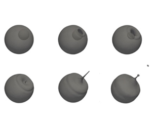
Figure 8 shows instantaneous images of the droplet morphology at different times. A bubble was initialized next to the droplet interface at a distance of  $50\ \mathrm {\mu }{\rm m}$. The bubble was expected to form by the evaporation of butanol as it was the more volatile component. The initial internal pressure of the bubble was calculated from the Young–Laplace equilibrium equation ( $\Delta P=\sigma /2R$). The bubble temperature was calculated from the pressure by using the SRK EoS. Droplet temperature was set equal to the boiling temperature of tetradecane (527 K) while the external temperature was prescribed at 700 K. The computational set-up adopted here was different from the experiment which used a heating coil below the particle and thus a spatial temperature gradient was expected. However, in the numerical simulation, an arbitrary ambient temperature was set at 700 K. This choice is justified because the time scale explored is short, and the characteristic size of the droplet resulted in negligible temperature gradients in the atmosphere; the difference between liquid and gas temperature generated boiling fluxes directed inward from the droplet to the bubble and outward from the droplet to the external atmosphere. A three-dimensional orthogonal mesh was used to simulate the reported cases. Each side of the cubic domain measured 2 mm, having $200\times 200\times 200$ cells. A grid convergence test showed that increased resolution did not substantially improve the results (figure 9).

Figure 8. Numerical simulation of the experiment performed by Rao et al. (Reference Rao, Karmakar and Basu2018) at  $\alpha _r=0.1$.

Figure 9. The numerical error associated with the grid resolution relative to the size of the ejected droplet for the case at  $\alpha =0.2$. The error is calculated as $\varepsilon =|(D_s^{n}-D_s^{e})/D_s^{e}|$, where the superscript $e$ indicates the experimentally measured values. Here $D/\Delta x$ is the ratio between the length of the domain and the side of each volume.
4.5.2. Interface collapse and jet formation
The pressure exerted from the bubble rapidly overcame the surface tension force, leading to a bubble collapse. The bubble collapse left a crater on the droplet's surface while capillary forces tended to re-establish the equilibrium of the droplet by recovering its spherical shape. This step visually agrees with the experimental observation of bubble burst (Lhuissier & Villermaux Reference Lhuissier and Villermaux2012; Gordillo & Rodríguez-Rodríguez Reference Gordillo and Rodríguez-Rodríguez2019). The experiment (Rao et al. Reference Rao, Karmakar and Basu2017) also reported the occurrence of Rayleigh–Taylor instability at the liquid–gas interface due to the density gradient. However, this was not observed in the numerical simulation mainly because it was conducted in microgravity conditions. Some researchers also mentioned the occurrence of evaporation-induced Darrieus–Landau instability at the bubble–droplet interface (Frost & Sturtevant Reference Frost and Sturtevant1986; Miglani, Basu & Kumar Reference Miglani, Basu and Kumar2014; Shinjo et al. Reference Shinjo, Xia, Ganippa and Megaritis2014) when explosive boiling occurred.
The pressure gradient also contributed to the crater shrinkage by pulling the mass of liquid outward. Following the gas ejection, capillary waves started to propagate through the droplet. A liquid ligament arose from the bottom of the crater at approximately  ${400}\ {\mathrm {\mu }{\rm s}}$. The ligament extended progressively, reaching the breakup point when the secondary droplet pinched off. Making use of the theoretical framework provided by Gañán Calvo (Reference Gañán Calvo2017) in his work on bubbles burst, the following correlation between jet velocity ( $V_{jet}$ and radius ( $R$) was used to compare the numerical results with the theory,
 \begin{equation} V_{jet} R_{jet}^{2} \sim R R_{jet}\sqrt{\sigma/(\rho R)}, \end{equation}
where  $R_{jet}$ is the radius of the cavity bottom at incipient jet formation and $R$ is the droplet radius. The numerical simulation scales well with the reported equation. For example, for $R_{jet}\sim R/10$ the jet velocity is estimated to be approximately ${0.2}\ {\rm m}\ {\rm s}^{-1}$, while the simulation predicted $V_{jet} = 0.18\ {\rm m}\ {\rm s}^{-1}$. Therefore, the simulation results agreed with the scaling relation. The jet velocity was calculated from the velocity profile along the axis expected for the ejection. In particular, for this purpose, a new variable was defined as the inner product between $\alpha _1$ and the velocity magnitude along the axis. That variable identified the value of liquid velocity. Plateau–Rayleigh instability was observed to be the dominant mechanism of droplet pinch-off (figure 8 at ${800}\ {\mathrm {\mu }{\rm s}}$), as confirmed by the experimental data. After breakup, the ligament retreated, while the surface continued to oscillate.
4.5.3. Comparison with experiments
A comparison between experimental and numerical results is reported in figures 10 and 11.

Figure 10. Comparison of simulation and experimental data Rao et al. (Reference Rao, Karmakar and Basu2017) for the size of the ejected droplet  $D_s$ as a function of the impact breakup parameter ( $\alpha _r$).

Figure 11. Comparison of simulation and experimental data Rao et al. (Reference Rao, Karmakar and Basu2017) for the breakup time,  $\tau _b$, as a function of impact breakup parameter ( $\alpha _r$). Breakup time is defined as the time occurring between ligament formation and its rupture to form the droplet.
The difference between experimental and numerical results is attributed to uncertainties in the measurements and necessary approximations in the case simulated. Experiments were performed in a suspended droplet facility with the fibre influencing the dynamics of the droplet. On the other hand, the numerical model considers a droplet in the absence of gravity with no fibre present. Another critical limitation is that the internal conditions were estimated from an equilibrium relation that does not hold in a boiling liquid having drastically changing properties. The initial temperature profile and homogeneous species distribution within the droplet were not known, therefore they were assumed uniform. The latter assumption had certainly a role in differentiating the numerical simulation from the experimental results. However, the obtained results demonstrate that the physics is satisfactorily captured from the numerical solver.
Another significant result was that initializing tiny bubbles, having an  $\alpha _r$ lower than 0.01, did not lead to ligament formation. This observation was reported in the work of Rao et al. (Reference Rao, Karmakar and Basu2017) and correctly captured by the present numerical simulation. It is therefore concluded that the geometric advection of the liquid–gas interface and the accurate estimation of the boiling fluxes are the main features required to quantify the degree of breakup of thermally induced atomization on this scale.
5. Results and discussion
The main results in this work are from conducting a series of simulations to predict different regimes of the atomization mechanism of HFO droplets. The fuel properties at  $50\,^{\circ }{\rm C}$ were measured in previous works (Khateeb et al. Reference Khateeb, Elbaz, Guida and Roberts2018; Jiang et al. Reference Jiang, Elbaz, Guida, Al-Noman, AlGhamdi, Saxena and Roberts2019) and are reported in table 1.
Table 1. Physical properties of the HFO used in this work at  $50\,^{\circ }{\rm C}$.

Given the strong temperature gradients within a droplet, temperature-dependent correlations for the physical properties were required. Viscosity was measured experimentally for HFO 380 as a temperature function, and a polynomial correlation was then extrapolated. Since mass transport and evaporation affect the local concentration of species, viscosity was also expected to be a function of mass fractions; however, in this work, the viscosity was assumed to be a function of temperature only. This assumption was necessary because mixing rules for such heavy components were not available, nor was any reasonably accurate chemical characterization of HFOs. The surface tension was calculated using the Riazi correlation (Riazi, Al-Sahhaf & Al-Shammari Reference Riazi, Al-Sahhaf and Al-Shammari1998) for petroleum fractions.
A series of simplifying assumptions used in the present simulations and relative justifications are summarized as follows.
(i) Microgravity was imposed. The Eötvös (Bond) number, defined as the ratio between gravitational and surface tension forces, is less than one for the cases analysed in this work. For example, an HFO droplet with a radius of 1 mm, surface tension of
${0.05}\ {\rm N}\ {\rm m}^{-1}$, a radius of curvature of 0.5 mm and density gradient of $1000\ {\rm kg}\ {\rm m}^{-3}$, has an Eötvös number of 0.05. This also explains the fact that HFO droplets maintain their spherical shape throughout the experiments when atomization does not occur (Khateeb et al. Reference Khateeb, Elbaz, Guida and Roberts2018; Jiang et al. Reference Jiang, Elbaz, Guida, Al-Noman, AlGhamdi, Saxena and Roberts2019).(ii) The presence of a thermocouple/fibre was neglected. The thermocouple is expected to trigger bubble nucleation through a heterogeneous nucleation mechanism. Its influence also affects the droplet temperature profile because its surface with high conductivity is easily heated by the external environment. However, since both temperature and bubble size were prescribed, and the simulations were performed in a short time, the role of the thermocouple may be considered negligible.
(iii) The HFO composition was simplified as a binary mixture, whose light fraction has the physical properties of diesel, and the heavy fraction has those of vacuum residue (VR).


A series of experiments preceded the computational campaign. The behaviour of HFO droplets exposed at high temperatures was tested on a suspended droplet facility. Details regarding the experimental set-up and the results obtained are reported elsewhere (Khateeb et al. Reference Khateeb, Elbaz, Guida and Roberts2018; Jiang et al. Reference Jiang, Elbaz, Guida, Al-Noman, AlGhamdi, Saxena and Roberts2019; Guida et al. Reference Guida, Saxena and Roberts2021). Figure 12 shows three photographs obtained from the experiments reported in a previous work (Guida et al. Reference Guida, Saxena and Roberts2021). The binary image in figure 12(a) demonstrates droplet ejection during puffing. The second snapshot reported in figure 12(b) represents the formation of the crater, while figure 12(c) shows the deformation of the droplet as a consequence of a microexplosion.

Figure 12. Binary images of experimental data (left) compared with the simulation at the matched condition (right). Thermocouple was removed from the picture during the post-processing. Experimental tests were performed on HFO droplets with a diameter of 1 mm exposed at a temperature of  $650\,^{\circ }{\rm C}$. Temperatures corresponding to the snapshots reported are (a) $315\,^{\circ }{\rm C}$, (b) $317\,^{\circ }{\rm C}$ and (c) $323\,^{\circ }{\rm C}$.
These instantaneous images were selected because ejection happened to be in a direction perpendicular to the camera. These three shapes also represent the typical characteristics of what the HFO droplet undergoes during the evaporation. As in the previous case, simulation was limited to the time during which atomization occurred. The total integration time was therefore set to 0.5 ms although the critical aspects of the atomization process were generally captured within 0.1 ms.
5.1. Case set-up
In the following parametric simulations, a droplet of HFO with a diameter of 1 mm was suspended in the absence of gravity (figure 13). The temperature of the ambient gas was kept constant at  $650\,^{\circ }{\rm C}$. The initial temperature of the liquid phase was assumed to be uniform at $380\,^{\circ }{\rm C}$, as measured by the thermocouple at the incipient breakup in the experiments. The evolution of the HFO droplet was studied for $\alpha _{r}$ coefficients ranging from 0.01 to 0.7.

Figure 13. Schematics of a case set-up. Ambient and droplet pressure are assumed to be equal:  $P_a=P_d=101.325\ {\rm Pa}$. Ambient temperature was $T_a= 650\,^{\circ }{\rm C}$ while temperature of droplet and bubble were assumed to be equal: $T_d=T_b= 300\,^{\circ }{\rm C}$. The mesh resolution is specified for each case. The boundaries are open, therefore a Neumann boundary condition is imposed by assuming the derivative of the variables with respect to the space equal to zero across the interface.
The bubble was assumed to be formed entirely by diesel fuel while the liquid was approximated as VR 60 % and diesel 40 % by mass. The critical properties adopted in the SRK EoS were evaluated using the correlations from Riazi et al. (Reference Riazi, Al-Sahhaf and Al-Shammari1998) for the VR, while the critical properties of n-eicosane ( ${\rm C}_{20}{\rm H}_{42}$) were used for diesel. Mass diffusivity and thermal conductivity were calculated according to empirical correlations as reported by Hentelä et al. (Reference Hentelä, Kaario, Garaniya, Goldsworthy and Larmi2017) for VR and on the Yaws (Reference Yaws2008) for diesel.
The breakup process followed different dynamics than in the benchmark case in § 4. Although the initial conditions were comparable, the physical properties of the fuels were substantially different because HFO presented higher surface tension and viscosity than butanol and tetradecane.
To quantify the increase in surface area of the droplet at different bubble sizes, a non-dimensional parameter called the breakup degree,  $B_d$, is defined as
 \begin{equation} B_d=\frac{S_{max}}{S_0}, \end{equation}
where  $S_{max}$ is the maximum surface area obtained and $S_0$ is the initial surface area. Figure 14 reports the results in terms of the breakup degree of five tests performed with different volume ratios, $\alpha _{r}$, defined in (1.5), where the volume of the droplet at incipient breakup is in the denominator.

Figure 14. Degree of breakup as a function of  $\alpha _r$.
Three distinct atomization mechanisms were identified depending on  $\alpha _r$. A small bubble ( $\alpha _r \sim 0.01$) resulted in simple ejection of vapours. At $\alpha _r \sim 0.1 - 0.6$, puffing was observed following a mechanism slightly different from that described by Rao et al. (Reference Rao, Karmakar and Basu2017). At $\alpha _r\sim 0.7$, microexplosion occurred, resulting in a much larger secondary surface area of approximately twice the initial size. These cases are described in detail in the following subsections, with particular attention devoted to the analysis of the interface collapse at incipient breakup.
5.2. Vapour ejection
At low  $\alpha _r$ ( ${\sim }0.01$), a rapid vapour ejection occurs. This is not a desirable condition in terms of atomization since it does not achieve the effective breakup of the droplet. At this condition, bubbles present high internal pressure concentrated in a small area, resulting in intense stress on the liquid meniscus that separates internal vapours and atmosphere. The curvature-driven drainage in the cap film was accelerated by the boiling process, which generated a mass flux directed both inward to the bubble centre and outward to the atmosphere. However, the boiling-flux contribution within the time scale in the conditions under investigation was negligible. A schematic representation of the physical phenomenon is shown in figure 15, where a cross-section of the droplet is reported. The geometric variables involved in the process are highlighted in a magnified snapshot.

Figure 15. Two-dimensional representation cross-section of the bubble representing the liquid meniscus before collapse. Letters indicating meniscus thickness (h), pinched region length (l) and pinching thickness ( $\delta$) recall the nomenclature adopted by Lhuissier & Villermaux (Reference Lhuissier and Villermaux2012).
The mass balance across the bubble cap is expressed by the following equation (Lhuissier & Villermaux Reference Lhuissier and Villermaux2012):
 \begin{equation} S\frac{{\rm d}h}{{\rm d}t}\sim Phu-\frac{\dot{m}_{v}}{\rho_l}, \end{equation}
where  $S$ and $P$ indicate the surface area and the perimeter of the bubble cap, while $h$,
$h$,  $u$ and $\dot {m}_{v}$ indicate, respectively, the cap thickness, the velocity component parallel to the bubble cap and the phase change flux. The values of $h$,
$h$,  $u$,
$u$,  $P$ and $S$, as well as the boiling flux $\dot {m}_{vap}$, were calculated from the simulation reported in figure 16. Considering an instant at which thickening occurred, the bubble cap thickness was approximately $h\sim 0.1\ {\rm mm}$, with a rate of ${\rm d}h/{\rm d}t \sim 0.1\ {\rm m}\ {\rm s}^{-1}$, and the ratio between perimeter and surface of the bubble cap was $P/S\sim 8\ {\rm mm}^{-1}$. The value of the velocity calculated from the numerical simulation was $u \sim 0.15\ {\rm m}\ {\rm s}^{-1}$. On the right-hand side of (5.2), the first term was therefore larger than the second term by two orders of magnitude; in fact, the boiling contribution was $\dot {m}_{vap}/(\rho _lS)\sim 2\ {\rm mm}\ {\rm s}^{-1}$. This implies that the mechanism that drove pinching at the bubble cap was curvature-driven drainage following the mechanism discussed by Lhuissier & Villermaux (Reference Lhuissier and Villermaux2012) in their work on the bursting of surface bubbles. Note that the velocity also scales well with the curvature-driven cap drainage velocity formulation proposed by Lhuissier & Villermaux (Reference Lhuissier and Villermaux2012),
 \begin{equation} u\sim{-}A\frac{\sigma}{\mu}\left(\frac{h}{R}\right)^{3/2} \end{equation}
where the coefficient  $A$ was found to be approximately 1.5.

Figure 16. Microgravity HFO droplet simulation at  $\alpha _r=0.01$.
In the numerical simulations with  $\alpha _r=0.01$, the collapse occurred through puncturing at the centre of the bubble (16). Once the liquid membrane collapsed, the pressure gradient led to a rapid gas ejection. The velocity of ejected gases was approximately $5\ {\rm m}\ {\rm s}^{-1}$. The droplet re-established its spherical shape through the effect of surface tension, generating capillary waves travelling across the surface.
5.3. Puffing
The second simulation case represents the puffing mode of atomization. Puffing is distinguished from the first mode in that a secondary droplet is ejected as a consequence of the rupture of the bubble cap. The bubble, initialized next to the interface ( $50\ \mathrm {\mu }{\rm m}$), expanded due to boiling flux coming from the liquid mixture of diesel and VR, which experienced an increasing temperature due to the hotter surrounding atmosphere. The size of the bubble cap was larger than the previous case, resulting in the formation of a pinching zone along a circular perimeter where the film of liquid connected to the rest of the droplet. The appearance of wrinkles at the interface anticipated the creation of a defined pinching region.
Figure 17 shows the fluctuations of the normalized magnitude of the radial component of the velocity from a top view, highlighting the formation and propagation of a crest that followed the disruption of the bubble cap. Wrinkles on the surface propagated and collapsed. The oscillations observed on the surface may be attributed to the Darrieus–Landau instability mechanism as suggested by previous studies (Shepherd & Sturtevant Reference Shepherd and Sturtevant1982; Frost & Sturtevant Reference Frost and Sturtevant1986; Shinjo et al. Reference Shinjo, Xia, Ganippa and Megaritis2014; Miglani et al. Reference Miglani, Basu and Kumar2014; Rao et al. Reference Rao, Karmakar and Basu2017). The Darrieus–Landau instability is triggered by the evaporative fluxes making the grooves of the liquid–atmosphere interface grow over time. The velocity gradients resulted in the formation of vortices forming in the gas phase above the bubble cap. The initial instability was dampened by surface tension, which played a significant role in the case of bubble eruption from heavy fuels.

Figure 17. Normalized velocity profile along a volume fraction isocontour ( $\alpha _r=0.42$); top view.
The structure of the bubble–droplet system after the initial instability corresponds to the condition observed in the previous case. However, the pinching zone was not confined to a single location, but was rather along the perimeter of the bubble cap, resembling the case of bursting surface bubbles. The numerical results were therefore compared again with the scaling proposed by Lhuissier & Villermaux (Reference Lhuissier and Villermaux2012). The following equation determines the relation between viscous dissipation and the pressure loss across the pinching region,
 \begin{equation} \frac{\mu{u}}{\delta^{2}}\sim\frac{\sigma}{R{l}}. \end{equation}
In the test simulation, the value of viscosity and surface tension were, respectively,  $\mu \sim 0.0325\ {\rm Pa}\ {\rm m}$ and $\sigma \sim 0.032\ {\rm N}\ {\rm m}^{-1}$, while velocity, radius and length of the pinching region were $\delta \sim 0.09\ {\rm mm}$, $R\sim 0.5\ {\rm mm}$ and $l\sim 0.2\ {\rm mm}$, resulting in a velocity approximately equal to $u\sim 0.1\ {\rm m}\ {\rm s}^{-1}$, in good agreement with the theory.
Figure 18 reports a three-dimensional representation of the puffing dynamics. The main difference in the vapour ejection here was that the fluid motion in the case of puffing proceeded in two directions, one towards the liquid meniscus and another directed to the centre of the bubble cap. The amount of liquid above the bubble increased as the pinching region shrunk until collapse occurred. This phenomenon is schematically shown in figure 19 as a two-dimensional projection of an isoalpha contour. The breakup process is clearly demonstrated by the truncation of the liquid meniscus and the formation of the droplet suspended above the cavity.

Figure 18. Microgravity HFO droplet puffing simulation with an  $\alpha _r=0.125$.

Figure 19. Two-dimensional projected interface evolution of microgravity HFO droplet at  $\alpha _r=0.42$.
The rupture of the liquid layer, after  $200\ \mathrm {\mu }{\rm s}$ in figure 18 following the stabilization of the pinching zone, accompanied a vapour jet formation. The fracture along the bubble cap perimeter formed a droplet in the shape of a prolate spheroid, suspended above the high-pressure cavity, which once consisted of the bubble. The vapour pushes the secondary particle away from the parent droplet while leaving the crater. The secondary droplet proceeded in its surface-tension-driven oscillatory dynamics following what was observed in the second benchmark case of nonlinear oscillations (figure 12a). When the bubble coalesced with the atmosphere, a capillary wave propagated through the bottom of the cavity. Edge regression re-established the spherical shape of the secondary droplet while a large jet arose from the cavity. Given that the size of the parent droplet was eventually of the same order of magnitude as the bubble, the jet drove the remaining fuel to deform the parent droplet itself (figure 12a).
The shape assumed by the droplet in figure 18 after  ${700}\ {\mathrm {\mu }}{\rm s}$ captures the experimental observation at similar conditions (figure 12b). The size of the jet radius was of the same order of magnitude as the bubble radius, therefore substantially more prominent than the case reported by Rao et al. (Reference Rao, Karmakar and Basu2017). The jet did not create any secondary droplet in the HFO droplets’ breakup due to pinching off of the liquid jet.
Gordillo & Rodríguez-Rodríguez (Reference Gordillo and Rodríguez-Rodríguez2019) stated that the jet velocity increases with the  $Oh$ number until a critical value ( $Oh_c$) is reached, after which the jet velocity becomes inversely proportional to the $Oh$ number. To clarify whether the case under study presented similar behaviour, a series of 4000 simulations at different $Oh$ values were executed. Figure 20 shows the scatter plot of the dataset, confirming the trend reported by Gordillo & Rodríguez-Rodríguez (Reference Gordillo and Rodríguez-Rodríguez2019) for microgravity droplet secondary breakup. A peak in $V_{jet}$ is found at approximately $Oh=0.03$, which is close to that found by Gordillo & Rodríguez-Rodríguez (Reference Gordillo and Rodríguez-Rodríguez2019). The transition point for the dependence of $V_{jet}$ on $Oh$ was found to depend on the initial size of the droplet, because the bubble size scales with the droplet size. The jet velocity decreased after the critical value, and together with the velocity decrease, the radius of the jet was expected to increase.

Figure 20. Jet velocity  $V_{jet}$ normalized with the capillary velocity for a series of 4000 simulations at different $Oh$ number and initial droplet size. The size of the droplet was in the range typical of sprays.
When the jet retracted into the parent droplet, a second capillary wave propagated, leading surface oscillations until a spherical shape was recovered. Puffing increased the exposed surface area by approximately 20 %–40 % of the initial surface and improved evaporation.
5.4. Microexplosions
The third and last case represented a microexplosion event. The expansion of a large bubble ( $\alpha _r=0.7$) resulted in simultaneously forming multiple ejection locations. The presence of more than one ejection site did not preclude the formation of a ligament in the parent droplet following a mechanism similar to single-site puffing. Figure 21 shows representative images during the atomization event and the evolution of the parent droplet. At $260\ \mathrm {\mu }{\rm s}$ a vapour jet arising from the bottom of the cavity drove a number of small ejected droplets. The simulation successfully reproduces the experimental observations made by the shadowgraph technique (figure 12c).

Figure 21. Microexplosion of HFO droplet at  $\alpha _r=0.7$.
Microexplosions represent the most favourable atomization mode with an increase in surface area of approximately two times for the conditions described above. The breakup degree  $B_d$ calculated on a large dataset (4000 simulations) is reported in figure 22. Cases that experienced microexplosions occurred at the low $Oh$ number and large initial diameters as indicated in the plot. The parametric study confirmed that larger bubbles resulted in more disruptive events, as observed in the complete simulations and in the experimental works.

Figure 22. Breakup degree  $B_{d}$ of a series of 4000 simulations at different $Oh$ number and initial droplet size $r_0$. Size of the droplet was kept in the size range typical of sprays.
6. Conclusions
A comprehensive high-fidelity computational simulation method was developed and implemented to predict and describe the complex physical phenomena associated with thermally induced secondary atomization of multicomponent liquids, allowing a realization of physically accurate behaviour for a wide range of parametric conditions, with accurate predictions of the secondary droplets size and breakup time scale. The present study demonstrated the role of simulations in complementing experimental limitations, allowing quantitative description of key observables, thus providing insights into underlying physical mechanisms.
Based on the OpenFOAM framework, a geometric VoF solver was improved to include the description of the phase change resulting from thermally induced evaporation and concentration-based mass diffusion. The PLIC–RDF reconstruction was adopted for accurate determination of the advection of the interface as well as the phase change source term and surface tension contribution, to our knowledge for the first time. The solver was validated against analytical solutions of various model problems, confirming that the solver can reproduce experiments reported in the literature.
The developed simulation tool was used to describe the physical behaviour of HFO droplets exposed to a high temperature, as a relevant practical application to showcase the capability of the advanced models. The fuel was described as a binary mixture of light (diesel) and heavy (VR) components. The code successfully predicted distinct phenomena observed in HFO atomization for different parametric regimes, consistent with the experimental findings (Khateeb et al. Reference Khateeb, Elbaz, Guida and Roberts2018; Jiang et al. Reference Jiang, Elbaz, Guida, Al-Noman, AlGhamdi, Saxena and Roberts2019; Guida et al. Reference Guida, Saxena and Roberts2021).
Note that the simulations in the present work were entirely deterministic. Nucleation, which is inherently a stochastic event, was thus not attempted. Previous studies (Klausner, Mei & Zeng Reference Klausner, Mei and Zeng1997; Liu & Dinh Reference Liu and Dinh2002; Mikami & Kojima Reference Mikami and Kojima2002) proposed a mathematical framework to describe the nucleation process, which may be adopted for future improvements
When available, the numerical simulation results were compared with the theoretical analysis, such as the bubble burst from a flat surface in term of the pinching mechanism (Lhuissier & Villermaux Reference Lhuissier and Villermaux2012), and jet formation (Gañán Calvo Reference Gañán Calvo2017) with the predicted scaling behaviour of relevant quantities (bubble cap thickening velocity ( $dh/dt$) and jet velocity ( $V_{jet}$)). The simulation also correctly reproduced the distinct jet velocity scaling with the Ohnesorge number below and above the critical value ( $Oh_c$), consistent with previous studies (Gordillo & Rodríguez-Rodríguez Reference Gordillo and Rodríguez-Rodríguez2019).
The present study also highlighted the differences between puffing in liquids with high and low surface tension. In the case of fuel having low surface tension (Rao et al. Reference Rao, Karmakar and Basu2017, Reference Rao, Karmakar and Basu2018), the droplet was formed from pinching the jet tip, following an instability of the Plateau–Rayleigh type. The atomization mechanism for HFO droplets was found to be different, in that the bubble cap drainage left a droplet on the surface, which was pushed outward from the gas trapped in the bubble. The initial mechanism of corrugation of the surface was explained as a manifestation of the Landau–Darrieus instability induced by the boiling fluxes at the liquid–atmosphere interface.
The parametric simulations demonstrated that the three distinct breakup regimes for the HFO droplet were accurately predicted depending on the ratio between bubble volume and droplet volume ( $\alpha _r$): a vapour ejection ( $\alpha _r< 0.015$); large bubbles and puffing ( $\alpha _r = 0.42$); and microexplosion ( $\alpha _r> 0.7$). Such a high level of fidelity allows the simulations to be a valuable design tool in predicting atomization behaviour of complex blend fuels consisting of heavy components for industrial applications.
Acknowledgements
The work was sponsored by the Clean Combustion Research Center at King Abdullah University of Science and Technology (KAUST). Computational resources were provided by the KAUST Supercomputing Laboratory (KSL).
Declaration of interests
The authors report no conflict of interest.
Appendix A. EoS
The SRK (Soave Reference Soave1972) equation was used to determine the fugacity coefficient of the mixture. The formula that allows to calculate the fugacity coefficient is the following:
 \begin{equation} \ln(\phi)=(Z-1)B_i/B-\ln(Z-B)-\frac{A}{2\sqrt{2}B}\left(\frac{2\sum x_iA_{i,j}}{A}- \frac{B_i}{B}\right)\ln\left(\frac{Z+(1+\sqrt(2)B}{Z+(1-\sqrt(2)B}\right) \end{equation}
where  $\phi$ is the fugacity coefficient, $Z$ is the compressibility factor and the coefficients $A$ and $B$ are
 \begin{gather} A_i=0.45724\frac{P_{r,i}}{T_{r,i}^{2}}, \end{gather}
 \begin{gather}A_{i,j}=(A_iA_j)^{1/2}, \end{gather}
 \begin{gather}B_i=0.0778\frac{P_{r,i}}{T_{r,i}}, \end{gather}
 \begin{gather}A=\sum^{NS}_{i=1}\sum^{NS}_{j=1}{x_ix_jA_{i,j}}, \end{gather}
 \begin{gather}B=\sum^{NS}_{i=1}{x_iB_i} \end{gather}
and the compressibility factor comes from the solution of the following equation:
 \begin{equation} Z^{3}+(1-B)Z^{2}+(A-3B^{2}-2B)Z+(B^{2}-AB+B^{3})=0. \end{equation}
The reduced temperatures  $T_{r,i}$ and $P_{r,i}$ are defined as $T_{r,i}=T/T_{c,i}$ and $P_{r,i}=P/P_{c,i}$. The subscript $i$ and $j$ indicate the different species while $x$ indicates the molar fractions in either liquid or gas phase.
Appendix B. Mixing rules
The mixing rules adopted are reported here for completeness. The thermal conductivity of the liquid mixture was calculated with the correlation proposed by Li (Reference Li1976),
 \begin{equation} k=\sum_{i=1}^{NS}\sum_{j=1}^{NS}\phi_i\phi_jk_{i,j} \end{equation}
where
 \begin{equation} \phi_i=\frac{x_iV_i}{\displaystyle\sum_{j=1}^{NS}x_jV_j} \end{equation}
and  $V_i$ is the molar volume of the ith component. The parameter $k_{i,j}$ was calculated as
 \begin{equation} k_{i,j}=\frac{2}{1/k_i+1/k_j}. \end{equation}
The mixing rule for viscosity was elaborated by Kendall & Monroe (Reference Kendall and Monroe1917) as follows:
 \begin{equation} \mu=\left(\sum_{i=1}^{NS}{x_i\mu_i^{1/3}}\right)^{3}, \end{equation}
where  $\mu _i$ is the viscosity of the ith component and $x_i$ its molar fraction. If not specified, a simple molar or mass average was used.


 Open access