


1. Introduction
1.1. Existence of transfer functions for time-varying base flows?
In the early stages of ‘natural’ (i.e. caused by small-amplitude two-dimensional Tollmien–Schlichting waves) laminar–turbulent transition of an incompressible flow on a smooth flat plate, the flow may be safely assumed to respond to perturbations in a linear time-invariant (LTI) fashion. Otherwise, the response of open shear flows to external excitations, even infinitesimal ones, is generally more complex. Turbulent flows certainly are not time-invariant, but neither are idealistic two-dimensional flows like the ones behind a backward-facing step or in the wake of one or a few cylinders at moderate Reynolds numbers. Even at very low Reynolds number, unsteadiness may set in as a result of noise amplification or intrinsic instability. Hence infinitesimal extrinsic perturbations interact not with a steady base flow but with a time-evolving one.
However, for feedback control using modern robust control techniques, an LTI model of the input–output dynamics is generally required. In the frequency domain, LTI dynamics indicates the existence of transfer functions, hence the question: how can we define transfer functions for time-varying, statistically steady base flows?
1.2. Option A: ‘dynamic linearity’, i.e. using small-amplitude harmonic forcings
Some authors have used harmonic forcings to identify transfer functions on simulations of statistically steady flows (Dahan, Morgans & Lardeau Reference Dahan, Morgans and Lardeau2012; Dalla Longa, Morgans & Dahan Reference Dalla Longa, Morgans and Dahan2017; Evstafyeva, Morgans & Dalla Longa Reference Evstafyeva, Morgans and Dalla Longa2017) that are either laminar or turbulent, and possess either peaked or broadband spectra. For sufficiently low forcing amplitude, the authors evaluate a frequency response by taking the ratio of the complex amplitudes of the output and input at the forcing frequency (the concept of nonlinear transfer function (Noiray et al. Reference Noiray, Durox, Schuller and Candel2008) is not relevant here due to the choice of low amplitude of the forcing). This observation hints at the existence of a transfer function in situations where it should not exist theoretically, given the time-varying nature of the base flow. The authors use the term ‘dynamic linearity’ to characterize this interesting behaviour, but no theoretical arguments seem available currently to understand it.
1.3. Option B: linearizing about the mean flow
A second option consists in assuming that the linear response  $\boldsymbol {u}$ to infinitesimal forcing $\boldsymbol {f}$ is characterized by the Jacobian matrix ${{\boldsymbol{\mathsf{J}}}}_{\bar {\boldsymbol {U}}}$ evaluated about the mean flow $\bar {\boldsymbol {U}}$, i.e.
 \begin{equation} \mathrm{d}_t\boldsymbol{u}={{\boldsymbol{\mathsf{J}}}}_{\bar{\boldsymbol{U}}}\boldsymbol{u}+\boldsymbol{f}.\end{equation}
As should be clear from (1.1), we adopt in this paper (except in Appendix C) a spatially discrete framework. The flow will be assumed incompressible and discretized over  $N$ degrees of freedom. The resolvent operator about the mean flow,
 \begin{equation} {{\boldsymbol{\mathsf{R}}}}_{\bar{\boldsymbol{U}}}(s)=(s{{\boldsymbol{\mathsf{I}}}}-{{\boldsymbol{\mathsf{J}}}}_{\bar{\boldsymbol{U}}})^{{-}1}, \end{equation}
then describes an LTI input–output dynamics in the frequency domain ( $s$ being the Laplace variable), and has been used successfully for open-loop (Moarref & Jovanović Reference Moarref and Jovanović2012; Luhar, Sharma & McKeon Reference Luhar, Sharma and McKeon2014; Toedtli, Luhar & McKeon Reference Toedtli, Luhar and McKeon2019; Yeh & Taira Reference Yeh and Taira2019; Liu et al. Reference Liu, Sun, Yeh, Ukeiley, Cattafesta and Taira2021) and closed-loop (Leclercq et al. Reference Leclercq, Demourant, Poussot-Vassal and Sipp2019) control of statistically steady flows. However, such an input–output model remains only empirically validated so far, and there is no clear justification for its use, since the mean flow is not an invariant solution of the nonlinear unforced system. The use of such a model is, however, motivated by a large body of literature devoted to linear analysis about a time-averaged mean flow, with clear predictive power.
Indeed, modal analysis of  ${{\boldsymbol{\mathsf{J}}}}_{\bar {\boldsymbol {U}}}$ yields accurate predictions of both the dominant oscillation frequency in the wake of a cylinder (Hammond & Redekopp Reference Hammond and Redekopp1997; Pier Reference Pier2002; Barkley Reference Barkley2006; Sipp & Lebedev Reference Sipp and Lebedev2007; Mittal Reference Mittal2008) and the associated coherent vortical structures. The growth rate of the leading eigenvalue, whose real part predicts the frequency, is nearly neutral, a property often called real zero imaginary frequency (RZIF; Turton, Tuckerman & Barkley Reference Turton, Tuckerman and Barkley2015; Bengana & Tuckerman Reference Bengana and Tuckerman2019, Reference Bengana and Tuckerman2021; Bengana et al. Reference Bengana, Loiseau, Robinet and Tuckerman2019), in a context that is now broader than just cylinder wake flow. This powerful property has been used to build self-consistent models (Mantič-Lugo, Arratia & Gallaire Reference Mantič-Lugo, Arratia and Gallaire2014, Reference Mantič-Lugo, Arratia and Gallaire2015; Meliga Reference Meliga2017; Bengana & Tuckerman Reference Bengana and Tuckerman2021) successfully mimicking the nonlinear flow with the simplest ingredients. The idea of marginal stability of the mean flow is not recent (Malkus Reference Malkus1956) but may be justified only under specific conditions, i.e. weak nonlinearity (Noack et al. Reference Noack, Afanasiev, Morzyński, Tadmor and Thiele2003; Sipp & Lebedev Reference Sipp and Lebedev2007), monochromatic oscillations (Mezić (Reference Mezić2013), criterion (b) of § 3.5; Turton et al. Reference Turton, Tuckerman and Barkley2015) or weak unsteadiness relative to the mean flow (Mezić (Reference Mezić2013), criterion (a) of § 3.5).
In the case of linearly stable flows, or noise-amplifiers, the resolvent operator about the turbulent mean flow has been used extensively to predict second-order statistics (Jovanovic & Bamieh Reference Jovanovic and Bamieh2001; Jovanovic & Georgiou Reference Jovanovic and Georgiou2010; Moarref et al. Reference Moarref, Jovanović, Tropp, Sharma and McKeon2014; Beneddine et al. Reference Beneddine, Sipp, Arnault, Dandois and Lesshafft2016; Zare, Jovanović & Georgiou Reference Zare, Jovanović and Georgiou2017; Towne, Lozano-Durán & Yang Reference Towne, Lozano-Durán and Yang2020) and in particular coherent flow structures characterized by spectral proper orthogonal decomposition (POD) modes (Semeraro et al. Reference Semeraro, Jaunet, Jordan, Cavalieri and Lesshafft2016a,Reference Semeraro, Lesshafft, Jaunet and Jordanb; Beneddine et al. Reference Beneddine, Sipp, Arnault, Dandois and Lesshafft2016; Schmidt et al. Reference Schmidt, Towne, Rigas, Colonius and Brès2018; Towne, Schmidt & Colonius Reference Towne, Schmidt and Colonius2018). The resolvent operator has also been used to obtain deterministic reduced-order models of unsteady flows from measurements of the mean flow and a few local probes (Gómez et al. Reference Gómez, Blackburn, Rudman, Sharma and McKeon2016; Beneddine et al. Reference Beneddine, Yegavian, Sipp and Leclaire2017; Symon, Sipp & McKeon Reference Symon, Sipp and McKeon2019). The input–output framework is also particularly fruitful for elucidating receptivity mechanisms through the analysis of the optimal forcing modes associated with the resolvent modes (Hwang & Cossu Reference Hwang and Cossu2010; Garnaud et al. Reference Garnaud, Lesshafft, Schmid and Huerre2013; Sartor, Mettot & Sipp Reference Sartor, Mettot and Sipp2015; Jeun, Nichols & Jovanović Reference Jeun, Nichols and Jovanović2016; Semeraro et al. Reference Semeraro, Lesshafft, Jaunet and Jordan2016b).
The intuition that coherent structures must extract their energy from the mean flow dates back to the contributions of Lee, Kim & Moin (Reference Lee, Kim and Moin1990), Butler & Farrell (Reference Butler and Farrell1993), Del Álamo & Jimenez (Reference Del Álamo and Jimenez2006), Cossu, Pujals & Depardon (Reference Cossu, Pujals and Depardon2009), Pujals et al. (Reference Pujals, García-Villalba, Cossu and Depardon2009) and McKeon & Sharma (Reference McKeon and Sharma2010) among others. However, despite the unchallenged efficacy of resolvent and modal analyses about the mean flow for modelling purposes, a clear justification for these procedures is still lacking (Beneddine et al. Reference Beneddine, Sipp, Arnault, Dandois and Lesshafft2016; Jovanović Reference Jovanović2021). As said already, the first difficulty in terms of interpretation arises from linearizing about a quantity, the mean flow, that is not an invariant solution of the governing equations. In the input–output framework of McKeon & Sharma (Reference McKeon and Sharma2010), the resolvent operator  ${{\boldsymbol{\mathsf{R}}}}_{\bar {\boldsymbol {U}}}$ is forced by a finite-amplitude internal forcing arising from nonlinear interactions of the perturbations. Although this framework is an exact reformulation of the Navier–Stokes equations, with no approximation involved, the procedure remains ad hoc in the sense that alternative formulations may be obtained by decomposing the flow about any alternative reference state, for instance the steady base flow. One practical reason for the popularity of this particular formulation is the recurrent observation that for energetic frequencies of the flow, the matrix ${{\boldsymbol{\mathsf{R}}}}_{\bar {\boldsymbol {U}}}(\mathrm {i}\omega )$ is often nearly rank 1, and the leading spectral POD mode is often well-approximated by the leading resolvent mode (Beneddine et al. Reference Beneddine, Sipp, Arnault, Dandois and Lesshafft2016; Towne et al. Reference Towne, Schmidt and Colonius2018). The clear advantage in this situation is that coherent flow structures may be predicted without having to consider the unknown nonlinear forcing term.
However, it is also increasingly clear that incorporating information about the nonlinear forcing into the linear operator, either in the form of an eddy viscosity (Illingworth, Monty & Marusic Reference Illingworth, Monty and Marusic2018; Morra et al. Reference Morra, Semeraro, Henningson and Cossu2019; Madhusudanan, Illingworth & Marusic Reference Madhusudanan, Illingworth and Marusic2019; Pickering et al. Reference Pickering, Rigas, Schmidt, Sipp and Colonius2021; Symon et al. Reference Symon, Sipp and McKeon2019), or through a low-rank state-feedback operator (Zare et al. Reference Zare, Jovanović and Georgiou2017), may significantly enhance its predictive power. For instance, the alignment between the leading resolvent mode and leading spectral POD mode may increase from 0.4 to nearly 0.9 by tuning the effective viscosity above the molecular viscosity (Pickering et al. Reference Pickering, Rigas, Schmidt, Sipp and Colonius2021). All these recent contributions confirm that  ${{\boldsymbol{\mathsf{R}}}}_{\bar {\boldsymbol {U}}}$ is a useful, yet suboptimal linear input–output representation. Worse still, (Karban et al. Reference Karban, Bugeat, Martini, Towne, Cavalieri, Lesshafft, Agarwal, Jordan and Colonius2020) showed recently that resolvent analysis about a mean flow is in general ill-posed as the poles of the operator depend on an arbitrary choice of formulation for the governing equations. In the case of a supersonic heated jet, discrepancies of up to $40\,\%$ were noted in the optimal gain at energetic frequencies, depending on the choice between the use of conservative versus primitive variables.
All these observations motivate the search for a new input–output operator, (i) incorporating information about the nonlinear forcings, (ii) which should be optimal in some sense, and (iii) which definition should be intrinsic. As we will see, the new operator will help us to understand the ‘dynamic linearity’ phenomenon and provide a physical interpretation to  ${{\boldsymbol{\mathsf{R}}}}_{\bar {\boldsymbol {U}}}$. Its poles will also exactly verify the RZIF property in the periodic case, whereas ${{\boldsymbol{\mathsf{R}}}}_{\bar {\boldsymbol {U}}}$ does so only approximately.
1.4. Option C: averaging the time-varying linear response
In this paper, we will not make the ad hoc hypothesis of linearity about the mean flow. We will keep only the assumption of linearity, which remains valid as long as the forcing amplitude is low enough, but now the base flow is an exact time-varying solution of the Navier–Stokes equations. Until § 4, the base flow will be assumed to be periodic with period  $T$ corresponding to a fundamental angular frequency $\omega _0:=2{\rm \pi} /T$. We represent in figure 1 the response $\boldsymbol {u}$ to an infinitesimal forcing signal $\boldsymbol {f}$ started at time $\tau _0$ relative to an arbitrary origin of time $\tau =0$ on the base flow trajectory $\tilde {\boldsymbol {U}}(\tau )$. Because the base flow is not steady but periodic, the linear response to forcing is not unique but parametrized by the phase $0\leqslant \phi <2{\rm \pi}$ of the limit cycle when the forcing starts. This key parameter for our analysis is defined such that
 \begin{equation} \omega_0\tau_0=\phi\text{ mod }2{\rm \pi}. \end{equation}
Indeed, the input–output dynamics is now characterized by a linear time-periodic (LTP) system
 \begin{equation} \mathrm{d}_t\boldsymbol{u}={{\boldsymbol{\mathsf{J}}}}(t;\phi)\,\boldsymbol{u}+\boldsymbol{f},\quad {{\boldsymbol{\mathsf{J}}}}(t+T;\phi)={{\boldsymbol{\mathsf{J}}}}(t;\phi),\end{equation}
with a periodic Jacobian itself parametrized by the phase  $\phi$ through the base flow $\boldsymbol {U}(t;\phi )={\tilde {\boldsymbol {U}}(\tau =t+\tau _0)}$. For $\phi$ distributed uniformly in $[0,2{\rm \pi} )$, there is in fact a distribution of time series $\boldsymbol {u}(t;\phi )$ corresponding to a given input $\boldsymbol {f}(t)$. The statistically optimal LTI approximation of this LTP system should predict a single output $\boldsymbol {v}(t)$ minimizing the mean error with respect to $\boldsymbol {u}(t;\phi )$, i.e.
 \begin{equation} \boldsymbol{v}(t)=\textrm{argmin}_{\tilde{\boldsymbol{v}}(t)}\lim_{T'\to\infty}\dfrac{1}{T'}\int_0^{T'} \langle\|\boldsymbol{u}(t;\phi)-\tilde{\boldsymbol{v}}(t)\|^2\rangle_\phi\,\mathrm{d}t, \end{equation}
where  $\langle \cdot \rangle _\phi$ denotes an ensemble average with respect to $\phi$. This output is obviously the mean response $\boldsymbol {v}(t)=\langle \boldsymbol {u}(t)\rangle _\phi$. We define the mean resolvent operator ${{\boldsymbol{\mathsf{R}}}}_0$ (the notation will become clear in § C.2) as the operator predicting the mean response, in the frequency domain, for any given input:
 \begin{equation} \boxed{\text{mean resolvent }{{\boldsymbol{\mathsf{R}}}}_0: \boldsymbol{f}(s)\mapsto\langle \boldsymbol{u}(s)\rangle_\phi}.\end{equation}
This transfer function is well-defined because the relationship between the input  $\boldsymbol {f}$ and the output $\langle \boldsymbol {u}\rangle _\phi$ is by construction causal, linear and time-invariant (i.e. independent of $\phi$).

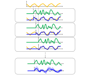
Figure 1. (a) Periodic base flow  $\tilde {\boldsymbol {U}}(\tau )$ for an arbitrarily defined origin of time $\tau =0$. (b) Linear responses $\boldsymbol {u}(t;\phi _i)$ to the same infinitesimal forcing $\boldsymbol {f}(t)$ started at different instants $\tau =\tau ^i_0$. Like the underlying base flow $\boldsymbol {U}(t;\phi _i)={\tilde {\boldsymbol {U}}(\tau =t+\tau ^i_0)}$, the responses are parametrized by the phase $\phi =\phi _i$ of the periodic base flow at $t=0$, such that $\omega _0\tau _0=\phi \text { mod }2{\rm \pi}$. (c) The response to linear forcing being a distribution, the statistically optimal LTI model is obtained by computing the mean response $\langle \boldsymbol {u}(t)\rangle _\phi$.
We see that in option C, the order of operations is reversed compared to option B: we linearize then average instead of averaging then linearizing. In option A, linearization is involved as well, but there is no averaging at all. Instead, a very specific form of input is chosen, which is harmonic in time. The three options are summarized in figure 2.

Figure 2. Three ways of defining an LTI operator for a periodic base flow.
1.5. Goal and outline of the paper
The aim of this paper is to investigate option C and establish connections with options A and B. In particular, we will show that option A is a specific way to evaluate  ${{\boldsymbol{\mathsf{R}}}}_0$, while ${{\boldsymbol{\mathsf{R}}}}_{\bar {\boldsymbol {U}}}$ is a (reduced-order) approximation of ${{\boldsymbol{\mathsf{R}}}}_0$, under appropriate conditions.
In §§ 2 and 3, we will continue to focus on incompressible periodic base flows. In § 2, we will perform a numerical experiment on the fluidic pinball in a periodic regime of oscillations at  $Re=100$, in order to compare options B and C, namely mean resolvent versus resolvent about the mean flow. In § 3, we will study the properties of the mean resolvent operator, with the goal to elucidate the observations made in § 2 and draw connections with the resolvent operator about the mean flow and ‘dynamic linearity’. Connections with the Koopman operator (§ 3.3), the RZIF property (§ 3.6) and model reduction (§ 3.5) will also be made. In § 4, we perform the same numerical experiment as in § 2 but for more complex base flows, i.e. quasi-periodic, chaotic and stochastic. We will consider the fluidic pinball at $Re=110$ and $Re=120$ as well as the backward-facing step flow (with exogenous stochastic forcing) at $Re=500$. The goal is to stress the strong connection between mean resolvent and resolvent about the mean flow in all these dynamically distinct cases. No computations are done in a compressible case, but in § 4.3 we indicate the implications of our theoretical analysis in § 3 to such situations. A theoretical extension of § 3 is proposed for the quasi-periodic case in Appendix D. We summarize our findings in § 5.
2. Resolvent about the mean flow versus mean resolvent: fluidic pinball at  $Re=100$

In this section, we perform a numerical experiment on the case of the incompressible two-dimensional fluidic pinball in a periodic regime at  $Re=100$. The goal is to compare transfer functions based on options B and C, i.e. average then linearize versus linearize then average. The precise configuration consists in the the numerical setting of Deng et al. (Reference Deng, Noack, Morzyński and Pastur2020). We define the unit length to be the diameter $D$ of each cylinder, and the (convective) time unit to be $D/U_\infty$, where $U_\infty$ is the upstream velocity norm. The Reynolds number is defined as $Re:=U_\infty D/\nu$, where $\nu$ is the kinematic viscosity. The centres of the ‘front’, ‘top’ and ‘bottom’ triangles are respectively located at $(x_f,y_f)=(-1.5\cos ({\rm \pi} /6),0)$, $(x_t,y_t)=(0,0.75)$ and $(x_b,y_b)=(0,-0.75)$, hence forming an equilateral triangle of side length $1.5$. Instead of measuring the full input–output relation between $N$-dimensional inputs and outputs, we will focus in this section on the single-input single-output (SISO) transfer between an actuator signal $u$ and a measurement $y$ such that
 \begin{equation} \boldsymbol{f}(t)=\boldsymbol{B}\,u(t),\quad y(t;\phi)=\boldsymbol{C}^T\,\boldsymbol{u}(t;\phi).\end{equation}
The SISO viewpoint is more practical for the numerical experiment that we perform, and it is also relevant in the context of flow control. More specifically, we will consider three probes  $\boldsymbol {C}$ extracting the $y$ velocity component in the wake of the ‘top’ cylinder at $y=y_t$ and respectively $x=2,4,8$ (white dots in figure 3). Measurements of the periodic base flow will be denoted $Y=\boldsymbol {C}^T\boldsymbol {U}$. When necessary, the index $a$,
$a$,  $b$ or $c$ will be used to specify which sensor we are referring to. The quantity $\boldsymbol {B}$ is a discretized Gaussian volume force field $\mathcal {B}(x,y;x_0,y_0,\sigma _x,\sigma _y)$ located at the ‘top’ of the ‘top’ cylinder:
 \begin{equation} \mathcal{B}(x,y;x_0,y_0,\sigma_x,\sigma_y)=\left[0,\exp\left({-\dfrac{(x-x_0)^2}{2\sigma_x^2}-\dfrac{(y-y_0)^2}{2\sigma_y^2}}\right)\right]^{\rm T},\end{equation}
with  $\sigma _x=0.01$, $\sigma _y=0.1$, and the centre $(x_0,y_0)$ of the Gaussian (white triangle in figure 3) relative to the centre $(x_t,y_t)$ of the cylinder being given by $(x_0-x_t,y_0-y_t)=(0,0.55)$.

Figure 3. Fluidic pinball at  $Re=100$, periodic behaviour: (a) mean velocity norm and streamlines, and(b) phase portraits using $y$ velocity sensors $Y_{b}$ and $Y_{c}$.
Numerical discretization details (computational domain, mesh, spatial and temporal schemes) are provided in Appendix A.
2.1. Unsteady base flow
In figure 3(a), we plot the streamlines and isocontours of velocity norm for the mean flow. We notice that it is asymmetric, as noted by Deng et al. (Reference Deng, Noack, Morzyński and Pastur2020). In figure 3(b), we plot the phase portrait of the flow, using the vertical velocity probes ‘b’ and ‘c’: it is a closed curve, which confirms the periodic nature of the dynamics at  $Re=100$. Fourier spectra are shown in row (i) of figure 5 for the three sensors (a–c) located in the wake of the cylinders. These spectra confirm the periodic nature of the flow since they are discrete with a single fundamental frequency at $\omega _0=0.73$ and harmonics. Higher frequencies are more energetic in the far wake than in the near wake. Indeed, perturbations amplify while being convected, causing stronger nonlinear energy transfers downstream.
2.2. Estimating mean transfer functions from input-output data
The resolvent operator about the mean flow  ${{\boldsymbol{\mathsf{R}}}}_{\bar {\boldsymbol {U}}}$ and the mean resolvent operator ${{\boldsymbol{\mathsf{R}}}}_0$ are both multiple-input multiple-output (MIMO) transfer functions with $N$-dimensional inputs and outputs. SISO transfer functions between any time-invariant actuator-sensor pair $(\boldsymbol {C},\boldsymbol {B})$ may be derived from these operators using
 \begin{equation} G_{\bar{\boldsymbol{U}}}(s):=\boldsymbol{C}^T{{\boldsymbol{\mathsf{R}}}}_{\bar{\boldsymbol{U}}}(s)\,\boldsymbol{B}\quad\text{and}\quad\langle G(s)\rangle_\phi:=\boldsymbol{C}^T{{\boldsymbol{\mathsf{R}}}}_0(s)\,\boldsymbol{B}. \end{equation}
In order to estimate the mean transfer function  $\langle G(s)\rangle _\phi$ from input–output data, we introduce ‘frequency response realizations’
 \begin{equation} G(s;\phi,u):=\dfrac{y(s;\phi)}{u(s)}, \end{equation}
which are obtained by taking the ratio between the Laplace transforms of the input  $u$ and the output $y$. The quantity $G$ is not associated directly with a transfer function since the linear response to forcing about a time-varying base flow is not time-invariant; hence the dependence on the phase $\phi$ and the input signal $u$. However, upon averaging with respect to $\phi$ (we recall that $\phi$ is assumed to be uniformly distributed in $[0,2{\rm \pi} )$), the linear input–output dynamics becomes time-invariant, and the dependence disappears. We then recover the mean transfer function based on the mean resolvent
 \begin{equation} \langle G(s)\rangle_\phi=\langle G(s;\phi,u)\rangle_\phi. \end{equation}
 For any complex frequency  $s$ and input signal $u$, the variance $\mathrm {Var}_\phi \,G(s;u)$ of the complex random variable $G(s;\phi,u)$ may be computed as
 \begin{align} \mathrm{Var}_\phi \,G&:=\langle |G -\langle G \rangle_\phi|^2\rangle_\phi\nonumber\\ &\phantom{:}= \langle |G|^2 \rangle_\phi - |\langle G \rangle_\phi|^2, \end{align}
and the ratio
 \begin{equation} \eta(s;u):=\dfrac{\sqrt{\mathrm{Var}_\phi\,{G}}}{|\langle G\rangle_\phi|}\end{equation}
may be interpreted as the inverse of a ‘signal-to-noise’ ratio, allowing us to quantify the validity of the time invariance hypothesis. The system is nearly LTI at a given frequency  $s$ if $\eta \ll 1$ for any choice of $u$. A geometric interpretation of $\eta$ will be proposed in figure 4.

Figure 4. Geometric interpretation of the ratio  $\eta$ for the three cases (a) $\eta \ll 1$, (b) $1<\eta <\sqrt {N_s}$ and (c) $\sqrt {N_s}\ll \eta$ of table 1; see main text for description.
The ratio  $\eta$ is also useful to evaluate the convergence of the mean estimate $\langle G\rangle _{\phi,N_s}$ to the true mean $\langle G\rangle _{\phi }$, using $N_s\gg 1$ realizations of $G$. Since all realizations are independent and identically distributed random variables of variance $\mathrm {Var}_\phi \,G$, the mean estimate is, by the central limit theorem, a normal random variable of variance
 \begin{equation} \mathrm{Var}_\phi\,\langle G\rangle_{\phi,N_s}=\dfrac{\mathrm{Var}_\phi\,G}{N_s}.\end{equation}
The convergence criterion  $\sqrt {\mathrm {Var}_\phi \,\langle G\rangle _{\phi,N_s} }\ll |\langle G \rangle _\phi |$ for the mean estimate therefore translates into the condition $\eta \ll \sqrt {N_s}$ for the given choice of $u$ and $s$.
$s$.
2.3. Procedure
The nonlinear simulation is initialized at  $\tau =0$ with the steady base flow (fixed point) perturbed by $\boldsymbol {B}$ (to quickly reach the limit cycle). After an initial transient of more than 1000 convective time units, the flow converges to a periodic regime of self-sustained oscillations.
This periodic base flow is then perturbed linearly using impulsive forcings  $u(t)=\delta (t)$ by simply initializing the perturbation field with the actuator, i.e. $\boldsymbol {u}(0)=\boldsymbol {B}$. Other choices of input signals may be made for estimating mean transfer functions, which will be discussed later, in §§ 3.2.2 and 3.2.3. Following impulsive forcing, both nonlinear (for the periodic base flow) and linear (for the perturbation) simulations are run for over more than 1000 convective time units. We compute $N_s=140$ impulse responses, by uniformly distributing the relative initial time $\tau _0$ over a period $T=8.64$ of the underlying limit cycle, i.e. $\Delta \tau _0=T/N_s$. This amounts to uniformly distributing the initial phase $\phi$ over $[0,2{\rm \pi} )$, as required.
Note that since impulse responses never decay, we can compute only frequency responses shifted in the right half-plane, i.e. obtained for  $s=\mathrm {i}\omega +\sigma$ with $\sigma >0$. This is indeed mandatory for convergence of the Laplace transform. The value $\sigma =0.01$ is chosen such that the mean impulse response modulated by $\mathrm {e}^{-\sigma t}$ reaches negligible values towards the end of the time window of 1000 convective time units. The Fourier transform of the exponentially modulated signal, estimated via the discrete Fourier transform, then yields the Laplace transform of the impulse over the shifted imaginary axis. The frequency response over $\mathrm {i}\mathbb {R}$ (minus the singularities) may then be retrieved by analytic continuation, but this is not done here.
The present analysis may remind the reader of the work by Yeh & Taira (Reference Yeh and Taira2019), who performed resolvent analysis about the mean flow on a shifted imaginary axis with  $\sigma >0$.
2.4. Results
First, a geometric interpretation of the ratio  $\eta$ is proposed in figure 4, where three cases are considered: (a) $\eta \ll 1$, (b) $1\leqslant \eta <\sqrt {N_s}$ and (c) $\sqrt {N_s} \ll \eta$, corresponding to the $\{\text {probe},\text {frequency}\}$ pairs of table 1. For a given value of $s$, the locus of $G(s;\phi )$ is represented by a closed blue curve in the complex plane as $\phi$ varies between 0 and $2{\rm \pi}$. The red dot indicates the barycentre of the curve, which is the estimated mean transfer $\langle G\rangle _{\phi,N_s}$. The length of the red arrow approximates $|\langle G\rangle _\phi |$. There are two dashed circles centred on the red dot: a black circle with radius approximating $\sqrt {\mathrm {Var}_\phi G}$ (length of black arrow), and a green circle with radius equal to $\sqrt {\mathrm {Var}_\phi \langle G\rangle _{\phi,N_s}}$ (length of green arrow). In figure 4(a), the radius of the black circle is much smaller compared to the red arrow, and the entire blue distribution may therefore be approximated by its red barycentre: the dynamics is quasi-time-invariant for that $\{\text {probe},\text {frequency}\}$ pair. In figure 4(b), the black arrow is twice the size of the red arrow, hence replacing the entire blue distribution by the single red dot is a very crude approximation: the dynamics is not quasi-time-invariant. However, the green arrow is still much smaller than the red arrow (see inset), which means that the estimation of the mean transfer function is converged. But in figure 4(c), not only is the black arrow much larger than the red arrow (dynamics not time-invariant), but the green arrow is also much larger than the red arrow (see inset), so there are not enough samples to estimate confidently the mean transfer function. We finally recall that only the exact mean $\langle G\rangle _\phi$ is independent from the forcing signal, while all other quantities (blue curve and its variance, mean transfer estimate and its variance) depend on the specific choice of $u(t)$.
Table 1. Values of the ratio  $\eta$ evaluated from $N_s=140$ impulses for three $\{\text {probe},\text {frequency}\}$ pairs.

We then proceed to a more systematic examination of  $\eta$ for $u(t)=\delta (t)$ in row (ii) of figure 5, for the three probes (a–c) over the frequency range $0\leqslant \omega \leqslant 10$. The threshold $\eta =1$ is indicated with a dashed black line, while the ratio $\eta =\sqrt {N_s}$ is indicated with a green dashed line. The value of $\eta$ with respect to these two critical values is also indicated in the Bode diagrams of the mean transfer function $\langle G\rangle _\phi$ represented in rows (iii) and (iv), for the gain and phase, respectively. No shading corresponds to a frequency range where $\eta < 1$, i.e. the dynamics is quasi-LTI; light-grey shading corresponds to $1\leqslant \eta <\sqrt {Ns}$, i.e. dynamics not LTI but mean estimate converged; and dark-grey shading corresponds to $\sqrt {N_s}\leqslant \eta$, i.e. mean estimate not even converged.

Figure 5. Fluidic pinball in the periodic regime at  $Re=100$. The labels (a)–(c) correspond to the three sensor positions. (i) Fourier spectrum of measurement $Y$ of the periodic base flow. The spectrum is discrete and no averaging is done, so a single Hann window is applied over the entire signal of more than 1000 time units. (ii) Ratio $\eta$ (defined in (2.7)) for $N_s=140$ impulsive forcings $u(t)=\delta (t)$. The black dashed line indicates the threshold $\eta =1$ far below which the system is nearly LTI (with respect to $u=\delta$). The green dashed line indicates the threshold $\eta =\sqrt {N_s}$ far below which the estimate of the mean transfer function is converged. Gain (iii) and phase (iv) of mean frequency response $\langle G\rangle _{\phi,N_s}$ (solid blue) and frequency response about the mean flow $G_{\bar {\boldsymbol {U}}}$ (dashed red). Light-grey shading indicates frequency ranges where $1< \eta <\sqrt {Ns}$, and dark-grey shading corresponds to $\eta \geqslant \sqrt {N_s}$. In the phase plots, the two black-dotted curves indicate a shift of $+/-{\rm \pi}$ with respect to the phase of $G_{\bar {\boldsymbol {U}}}$. For rows (ii), (iii) and (iv), all quantities are evaluated on the shifted imaginary axis $\sigma +\mathrm {i}\omega$, with $\sigma =0.01$.
The first remark is that the ratio  $\eta$ becomes larger as the probe moves downstream. As a result, converging the mean transfer estimate requires more samples downstream than upstream (see greater extent of dark-grey regions). Correlatively, the frequency range of validity of the quasi-time-invariant region shrinks as the probe moves downstream. Both observations seem correlated with the fact that the unsteady fluctuations are more energetic downstream than upstream (see power spectra in row (i) of figure 5). The ratio $\eta$ is also greater near resonance frequencies for the same reason: the base flow fluctuations are greater near these frequencies. It is interesting to note, however, that for all probe positions, the LTI approximation is valid in some frequency range near the maximum gain (but excluding resonances).
Whether or not  $\eta$ is small compared to 1, we always observe a qualitative agreement between the Bode diagrams of $G_{\bar {\boldsymbol {U}}}$ and $\langle G\rangle _{\phi }$, as long as the mean estimate is converged. For probe a, the two diagrams are nearly indistinguishable from one another, and the deviation remains very small for probe b as well, except near resonant frequencies $k\omega _0$. For probe c, though, the deviation becomes noticeable, even when $\eta <1$.
Only the fundamental frequency leads to a resonance peak in  $G_{\bar {\boldsymbol {U}}}$, whereas higher-order harmonics are also visible in $\langle G\rangle _\phi$. These extra peaks are indicative of the presence of poles at $s=\mathrm {i}k\omega _0$ in the mean transfer function, but the amplitude of the peaks decreases rapidly with $k$ and as the probe moves upstream.
In § 3, we will attempt to elucidate the aforementioned observations. (i) Why are  $\langle G\rangle _\phi$ and $G_{\bar {\boldsymbol {U}}}$ generally so similar? (ii) Why does the quality of the LTI approximation deteriorate downstream? (iii) Why are there poles at $s=\mathrm {i}k\omega _0$ in the mean transfer function? (iv) Why are higher-order resonances weaker and noticeable only downstream?
3. Theory for incompressible periodic base flows
In this theoretical section, we come back to the more general MIMO viewpoint between an  $N$-dimensional forcing $\boldsymbol {f}(t)$ and an $N$-dimensional response $\boldsymbol {u}(t;\phi )$.
3.1. Phase-dependent frequency response of an LTP system
Denote by  $\boldsymbol {\varPhi }(t,t';\phi )$ the propagator from $t'$ to $t$ of the linear time-periodic system (1.4a,b), such that
 \begin{equation} \boldsymbol{u}(t;\phi)=\boldsymbol{\varPhi}(t,0;\phi)\,\boldsymbol{u}_0+\int_{0}^t \boldsymbol{\varPhi}(t,t';\phi)\,\boldsymbol{f}(t')\,\mathrm{d}t',\end{equation}
where  $\boldsymbol {u}_0$ is the initial condition on $\boldsymbol {u}$, regardless of $\phi$. By Floquet's theorem (Magruder, Gugercin & Beattie Reference Magruder, Gugercin and Beattie2018), we know that there exists a real $T$-periodic matrix ${{\boldsymbol{\mathsf{P}}}}(t;\phi )$, invertible at all times $t$, and a constant complex matrix ${{\boldsymbol{\mathsf{K}}}}$ such that $\boldsymbol {\varPhi }(t,t';\phi )={{\boldsymbol{\mathsf{P}}}}(t;\phi )\,\mathrm {e}^{{{\boldsymbol{\mathsf{K}}}}(t-t')}\,{{\boldsymbol{\mathsf{P}}}}^{-1}(t';\phi )$. There are multiple possible determinations of the matrix ${{\boldsymbol{\mathsf{K}}}}=(1/T)\log (\boldsymbol {\varPhi }(T,0))$ depending on the definition of the logarithm. Assuming ${{\boldsymbol{\mathsf{K}}}}$ to be diagonalizable, ${{\boldsymbol{\mathsf{K}}}}={{\boldsymbol{\mathsf{S}}}}\boldsymbol {\varLambda }{{\boldsymbol{\mathsf{S}}}}^{-1}$, and choosing the principal determination for the logarithm, all the eigenvalues fall into the fundamental strip $-\omega _0/2<\mathrm {Im}(\lambda _i)\leqslant \omega _0/2$, $i=1,\dots,N$. These are called the principal Floquet exponents, and they may be ranked in decreasing order of growth rate, i.e. $\mathrm {Re}(\lambda _1)\geqslant \mathrm {Re}(\lambda _2) \geqslant \cdots \geqslant \mathrm {Re}(\lambda _N)$. Other determinations of the logarithm lead to eigenvalues $s_{ij}=\lambda _i+\mathrm {i}j\omega _0$ which are Floquet exponents as well, located in complementary strips $\omega _0(j-1/2)<\mathrm {Im}(s_{ij})\leqslant \omega _0(j+1/2)$ in the complex plane. The direct Floquet modes $\boldsymbol {v}^i$ are the columns of the $T$-periodic complex matrix ${{\boldsymbol{\mathsf{V}}}}(t;\phi ):={{\boldsymbol{\mathsf{P}}}}(t;\phi ){{\boldsymbol{\mathsf{S}}}}$. The adjoint Floquet modes $\boldsymbol {w}^i$, such that $(\boldsymbol {w}^i,\boldsymbol {v}^j)=\delta _{ij}$ for the canonical inner product $(\boldsymbol {a},\boldsymbol {b})=1/T\int _0^T\boldsymbol {a}^H\boldsymbol {b}\,\mathrm {d}t$ on the space of periodic functions in $\mathbb {C}^N$ (where $^H$ denotes the complex transpose), are the columns of the matrix ${{\boldsymbol{\mathsf{W}}}}(t;\phi )$ such that ${{\boldsymbol{\mathsf{W}}}}^H{{\boldsymbol{\mathsf{V}}}}={{\boldsymbol{\mathsf{I}}}}$ at all times (and phases $\phi$). Using this eigendecomposition, the propagator reads
 \begin{equation} \boldsymbol{\varPhi}(t,t';\phi)={{\boldsymbol{\mathsf{V}}}}(t;\phi)\,\mathrm{e}^{\boldsymbol{\varLambda} (t-t')}\, {{\boldsymbol{\mathsf{W}}}}^H(t';\phi).\end{equation}
We may now expand the direct and adjoint Floquet modes as Fourier series. If the  $j\text {th}$ Fourier coefficient of ${{\boldsymbol{\mathsf{V}}}}$ is proportional to $\mathrm {e}^{\mathrm {i}j\phi }$, then so is the $j\text {th}$ Fourier coefficient of ${{\boldsymbol{\mathsf{W}}}}$ since ${{\boldsymbol{\mathsf{W}}}}^H{{\boldsymbol{\mathsf{V}}}}={{\boldsymbol{\mathsf{I}}}}$ at all times. Therefore, we can write the following Fourier series:
 \begin{equation} {{\boldsymbol{\mathsf{V}}}}(t;\phi)=\sum_j \hat{{{\boldsymbol{\mathsf{V}}}}}_j \exp({\mathrm{i}j(\omega_0 t+\phi)}),\quad {{\boldsymbol{\mathsf{W}}}}(t';\phi)=\sum_j \hat{{{\boldsymbol{\mathsf{W}}}}}_j \exp({\mathrm{i}j(\omega_0 t'+\phi)}). \end{equation}
Injecting (3.2) and (3.3a,b) in (3.1) and assuming  $\boldsymbol {u}_0=\boldsymbol {0}$, we have
 \begin{align}
&\boldsymbol{u}(t;\phi)\nonumber\\ &\quad=\int_{0}^t
{{\boldsymbol{\mathsf{V}}}}(t;\phi)\exp({\boldsymbol{\varLambda}
(t-t')})\,
{{\boldsymbol{\mathsf{W}}}}^H(t';\phi)\,\boldsymbol{f}(t')\,\mathrm{d}t'\nonumber\\
&\quad=\int_{0}^t \left[\sum_j
\hat{{{\boldsymbol{\mathsf{V}}}}}_j\exp({\mathrm{i}j(\omega_0t\,{+}\,\phi)})\right]
\exp({\boldsymbol{\varLambda}(t\,{-}\,t')})\left[\sum_l
\hat{{{\boldsymbol{\mathsf{W}}}}}^H_l\exp({-\mathrm{i}l(\omega_0t'\,{+}\,\phi)})\right]
\boldsymbol{f}(t')\,\mathrm{d}t'\nonumber\\
&\quad=\sum_{j,l}\exp({\mathrm{i}(j-l)\phi})\int_{0}^t\left[
\hat{{{\boldsymbol{\mathsf{V}}}}}_j
\exp({(\boldsymbol{\varLambda}+\mathrm{i}j\omega_0{{\boldsymbol{\mathsf{I}}}})(t-t')})\,
\hat{{{\boldsymbol{\mathsf{W}}}}}^H_l\right]\left[\exp({\mathrm{i}(j-l)\omega_0
t'})\,\boldsymbol{f}(t')\right]\mathrm{d}t'\nonumber\\
&\quad=\sum_{n}\exp({\mathrm{i}n\phi})\int_{0}^t\left[\sum_{j}\hat{{{\boldsymbol{\mathsf{V}}}}}_j
\exp({(\boldsymbol{\varLambda}+\mathrm{i}j\omega_0{{\boldsymbol{\mathsf{I}}}})(t-t')})\,
\hat{{{\boldsymbol{\mathsf{W}}}}}^H_{j-n}\right]\left[\exp({\mathrm{i}n\omega_0
t'})\,\boldsymbol{f}(t')\right]\mathrm{d}t'.
\end{align}
\begin{align}
&\boldsymbol{u}(t;\phi)\nonumber\\ &\quad=\int_{0}^t
{{\boldsymbol{\mathsf{V}}}}(t;\phi)\exp({\boldsymbol{\varLambda}
(t-t')})\,
{{\boldsymbol{\mathsf{W}}}}^H(t';\phi)\,\boldsymbol{f}(t')\,\mathrm{d}t'\nonumber\\
&\quad=\int_{0}^t \left[\sum_j
\hat{{{\boldsymbol{\mathsf{V}}}}}_j\exp({\mathrm{i}j(\omega_0t\,{+}\,\phi)})\right]
\exp({\boldsymbol{\varLambda}(t\,{-}\,t')})\left[\sum_l
\hat{{{\boldsymbol{\mathsf{W}}}}}^H_l\exp({-\mathrm{i}l(\omega_0t'\,{+}\,\phi)})\right]
\boldsymbol{f}(t')\,\mathrm{d}t'\nonumber\\
&\quad=\sum_{j,l}\exp({\mathrm{i}(j-l)\phi})\int_{0}^t\left[
\hat{{{\boldsymbol{\mathsf{V}}}}}_j
\exp({(\boldsymbol{\varLambda}+\mathrm{i}j\omega_0{{\boldsymbol{\mathsf{I}}}})(t-t')})\,
\hat{{{\boldsymbol{\mathsf{W}}}}}^H_l\right]\left[\exp({\mathrm{i}(j-l)\omega_0
t'})\,\boldsymbol{f}(t')\right]\mathrm{d}t'\nonumber\\
&\quad=\sum_{n}\exp({\mathrm{i}n\phi})\int_{0}^t\left[\sum_{j}\hat{{{\boldsymbol{\mathsf{V}}}}}_j
\exp({(\boldsymbol{\varLambda}+\mathrm{i}j\omega_0{{\boldsymbol{\mathsf{I}}}})(t-t')})\,
\hat{{{\boldsymbol{\mathsf{W}}}}}^H_{j-n}\right]\left[\exp({\mathrm{i}n\omega_0
t'})\,\boldsymbol{f}(t')\right]\mathrm{d}t'.
\end{align}
We recognize convolution products of causal functions on the right-hand side, hence it is easy to take the Laplace transform, yielding the linear time-periodic input–output relation
 \begin{equation} \boxed{ \boldsymbol{u}(s;\phi)=\sum_n \mathrm{e}^{\mathrm{i}n\phi}\,{{\boldsymbol{\mathsf{R}}}}_n(s)\,\boldsymbol{f}(s-\mathrm{i}n\omega_0)},\end{equation}
with the operators
 \begin{equation} \boxed{ {{\boldsymbol{\mathsf{R}}}}_n(s)=\sum_j \sum_{k=1}^N\dfrac{ \hat{\boldsymbol{v}} ^k_j{(\hat{\boldsymbol{w}}^k_{j-n})^H} }{s-(\lambda_k+\mathrm{i}j\omega_0)}},\end{equation}
where  $\hat {\boldsymbol {v}}^k_j$ and $\hat {\boldsymbol {w}}^k_j$ designate the $k\text {th}$ columns of $\hat {{{\boldsymbol{\mathsf{V}}}}}_j$ and $\hat {{{\boldsymbol{\mathsf{W}}}}}_j$. Unlike in LTI systems, the output at frequency $s$ depends on the input at an infinite number of frequencies $s-\mathrm {i}n\omega _0$. The output depends explicitly on the phase $\phi$ through the cross-frequency transfers $\mathrm {e}^{\mathrm {i}n\phi }\,{{\boldsymbol{\mathsf{R}}}}_n(s)$ for $n\neq 0$. The poles of the ${{\boldsymbol{\mathsf{R}}}}_n$ are exactly the Floquet exponents of the LTP system. The adjoint Floquet modes characterize receptivity to forcing of the corresponding direct Floquet modes.
3.2. Mean resolvent operator
We now seek the operator that predicts the mean output  $\langle \boldsymbol {u}(s)\rangle _\phi$ for a given input $\boldsymbol {f}(s)$, by averaging (3.5) with respect to $\phi$. By doing so, all the cross-frequency transfers vanish, and the only remaining transfer is ${{\boldsymbol{\mathsf{R}}}}_0$:
 \begin{equation} \boxed{ \langle \boldsymbol{u}(s)\rangle_\phi={{\boldsymbol{\mathsf{R}}}}_0(s)\,\boldsymbol{f}(s)}, \end{equation}
which is consistent with our initial choice of notation for the mean resolvent in the Introduction.
3.2.1. Resonances at natural frequencies
Next, we note that since the periodic base flow  $\boldsymbol {U}(t)$ is self-sustained (no external forcing is required), there is a zero Floquet exponent in the LTP system with associated Floquet mode equal to $\mathrm {d}_t \boldsymbol {U}$ (see Appendix B). If we restrict our attention to the case where the periodic base flow is linearly stable, then the zero Floquet exponent is the leading one, i.e. $\lambda _1=0$ and $\boldsymbol {v}^1=\mathrm {d}_t \boldsymbol {U}$ (in case of instability $\lambda _1>0$ but there is still a zero exponent $\lambda _j=0$ for some $j>1$), so that $\hat {\boldsymbol {v}}^1_j=\mathrm {i}j\omega _0\hat {\boldsymbol {U}}_j$, where $\hat {\boldsymbol {U}}_j$ denotes the $j\text {th}$ harmonic of the Fourier decomposition of $\boldsymbol {U}(t)$. Therefore, using expression (3.6), the mean resolvent reads
 \begin{equation} \boxed{ {{\boldsymbol{\mathsf{R}}}}_0(s)=\sum_{j\neq0}\dfrac{ \mathrm{i}j\omega_0\,{\hat{\boldsymbol{U}}}_j(\hat{\boldsymbol{w}}^1_j)^H }{s-\mathrm{i}j\omega_0}+\sum_j\sum_{k=2}^N\dfrac{ \hat{\boldsymbol{v}} ^k_j(\hat{\boldsymbol{w}}^k_j)^H }{s-(\lambda_k+\mathrm{i}j\omega_0)}}. \end{equation}
We see immediately that there are purely imaginary poles at  $s=\mathrm {i}j\omega _0$, as expected from the numerical experiment on the fluidic pinball. The coefficients associated with these poles in the expansion, also called the residuals
 \begin{equation} \mathrm{Res}_{\mathrm{i}j\omega_0}\,{{\boldsymbol{\mathsf{R}}}}_0(s)=\mathrm{i}j\omega_0\,{\hat{\boldsymbol{U}}}_j(\hat{\boldsymbol{w}}^1_j)^H, \end{equation}
tend very rapidly to 0 in the operator norm as  $|j|\to \infty$, because the $j\text {th}$ Fourier harmonics of both $\boldsymbol {U}$ and $\boldsymbol {w}^1$ are involved (the decay is $o(1/j^m)$ for any integer $m$ if we consider $\mathcal {C}^\infty$ periodic structures). This explains why resonance peaks caused by imaginary poles in figure 5(ii) become decreasingly visible as $|j|$ increases. The fact that the residuals depend on $\hat {\boldsymbol {U}}_j$ also explains why resonances at high frequencies are, however, more visible downstream than upstream. Indeed, larger oscillation amplitude in the far wake causes more pronounced nonlinear energy transfers to higher harmonics (see base flow spectra in figure 5(i)), hence a better observability $|\boldsymbol {C}^T\hat {\boldsymbol {U}}_j|$ of high-order harmonics $\hat {\boldsymbol {U}}_j$ as the sensor moves downstream.
3.2.2. System identification using frequency-rich inputs
The upside of using frequency-rich signals for system identification is that it allows us to identify the dynamics for multiple frequencies at once. The downside, though, is that many realizations of the same input signal may be necessary to converge the mean response prior to identification, as we have seen in § 2 (in particular row (iv) in figure 5). The number of realizations necessary to converge the mean is very dependent on the input signal chosen. This dependence can be made explicit, using (3.5) and the definition of the variance:
 \begin{equation} \mathrm{Var}_\phi\,\boldsymbol{u}(s)=\sum_{n\neq 0}\|\boldsymbol{f}(s-\mathrm{i}n\omega_0)\|_{{{\boldsymbol{\mathsf{R}}}}_n^H{{\boldsymbol{\mathsf{R}}}}_n}^2,\end{equation}
where  $\|\boldsymbol {a}\|_{{{\boldsymbol{\mathsf{M}}}}}=(\boldsymbol {a}^H{{\boldsymbol{\mathsf{M}}}}\boldsymbol {a})^{1/2}$ is the norm induced by the positive-definite matrix ${{\boldsymbol{\mathsf{M}}}}$. A convenient choice of input signal is one that minimizes the variance, allowing for a minimal amount of realizations. Clearly, an input signal with a broadband spectrum like an impulse $\boldsymbol {f}(t)=\boldsymbol {B}\,\delta (t)$ (for which $\delta (s)=1$ for all $s$) is likely to generate a lot of output variance and is not necessarily a favourable choice for identification. An alternative to frequency-rich inputs is to use non-resonant harmonic forcings for identification, as we will see in the next subsubsection.
Another advantage of using a broadband input signal for identification is that if the ratio  $\eta$ is very small compared to 1 for such an input signal, then the ratio is likely to be very small for any input signal, hence the LTI approximation based on the mean response is likely to be meaningful. Expression (3.10) also explains why the quality of the LTI approximation deteriorates as the sensor moves downstream in figure 5(iv) for $u(t)=\delta (t)$. Indeed,
 \begin{equation} \mathrm{Var}_\phi\,G(s;u=\delta)=\sum_{n\neq 0} | \boldsymbol{C}^T{{\boldsymbol{\mathsf{R}}}}_n(s)\,\boldsymbol{B}|^2, \end{equation}
which, according to (3.6), increases downstream since the observability  $|\boldsymbol {C}^T\hat {\boldsymbol {v}}_j^k|$ of the Floquet modes probably grows downstream (this is obvious for the first Floquet mode since $\hat {\boldsymbol {v}}^1_j=\mathrm {i}j\omega _0\hat {\boldsymbol {U}}_j$).
3.2.3. System identification using harmonic inputs: ‘dynamic linearity’
The Laplace transform of harmonic forcings of the form  $\boldsymbol {f}(t)=\boldsymbol {B}\,\mathrm {e}^{\mathrm {i}\omega t}$ is given by
 \begin{equation} \boldsymbol{f}(s)=\dfrac{\boldsymbol{B}}{s-\mathrm{i}\omega}. \end{equation}
Plugging this expression into the input–output relation (3.5) leads to
 \begin{equation} \boldsymbol{u}(s;\phi)=\sum_n \mathrm{e}^{\mathrm{i}n\phi}\,\dfrac{{{\boldsymbol{\mathsf{R}}}}_n(s)\,\boldsymbol{B}}{s-\mathrm{i}(\omega+n\omega_0)}.\end{equation}
The temporal response may now be evaluated by inverting the Laplace transform. For the linearly stable limit cycle considered here, the decaying Floquet exponents lead to a transient response, while all the purely imaginary poles in the right-hand side of (3.13), in either the transfer operators or the forcing, lead to a permanent contribution. For non-resonant forcing frequencies  $\omega \neq n\omega _0$, we have
 \begin{align} \boldsymbol{u}(t;\phi)&=\mathrm{transient}\nonumber\\ &\quad+{{\boldsymbol{\mathsf{R}}}}_0(\mathrm{i}\omega)\,\boldsymbol{B}\exp({\mathrm{i}\omega t})+\sum_{j\neq 0}\mathrm{i}j\omega_0\,\hat{\boldsymbol{U}}_j(\hat{\boldsymbol{w}}_j^1)^H\boldsymbol{B} \exp({\mathrm{i}j\omega_0t})\nonumber\\ &\quad+\sum_{n\neq 0}\exp({\mathrm{i}n\phi})\left[\vphantom{\sum_{n\neq 0}} {{\boldsymbol{\mathsf{R}}}}_n(\mathrm{i}(\omega+n\omega_0))\,\boldsymbol{B} \exp({\mathrm{i}(\omega+n\omega_0)t})\right.\nonumber\\ &\quad \left.+\sum_{j\neq 0}\mathrm{i}j\omega_0\, \hat{\boldsymbol{U}}_j(\hat{\boldsymbol{w}}_{j-n}^1)^H\boldsymbol{B} \exp({\mathrm{i}j\omega_0t})\right]. \end{align}
The first line of (3.14) collects the transient contributions, and the second line gathers terms that are phase-independent, while the third line is phase-dependent and vanishes upon averaging. However, the point here is not to take an average but to notice that the Fourier coefficient at the forcing frequency, which may be obtained using a harmonic average
 \begin{equation} \hat{\boldsymbol{u}}(\omega;\phi)=\lim_{T'\to \infty}\dfrac{1}{T'}\int_0^{T'} \boldsymbol{u}(t;\phi)\,\mathrm{e}^{-\mathrm{i}\omega t}\,\mathrm{d}t, \end{equation}
is phase-independent and given exactly by the product of the input amplitude  $\hat {\boldsymbol {f}}(\omega )=\boldsymbol {B}$ by the mean resolvent operator evaluated at $s=\mathrm {i}\omega$:
 \begin{equation} \boxed{\hat{\boldsymbol{u}}(\omega)={{\boldsymbol{\mathsf{R}}}}_0(\mathrm{i}\omega)\,\hat{\boldsymbol{f}}(\omega) }. \end{equation}
 In other terms, using small-amplitude harmonic forcings, it is possible to obtain frequency samples of the mean transfer function  $\langle G\rangle _\phi =\boldsymbol {C}^T{{\boldsymbol{\mathsf{R}}}}_0\boldsymbol {B}$ without the need to carry out an ensemble average over several realizations. This is in essence the ‘dynamic linearity’ phenomenon described by Dahan et al. (Reference Dahan, Morgans and Lardeau2012), Dalla Longa et al. (Reference Dalla Longa, Morgans and Dahan2017) and Evstafyeva et al. (Reference Evstafyeva, Morgans and Dalla Longa2017), and used therein for LTI system identification on time-varying base flows.
In principle, using a superposition of harmonic forcings
 \begin{equation} \boldsymbol{f}(t)=\boldsymbol{B}(A_1\,\mathrm{e}^{\mathrm{i}\omega_1 t}+A_2\,\mathrm{e}^{\mathrm{i}\omega_2 t}+\cdots), \end{equation}
it should even be possible to sample the mean transfer function at all input frequencies at once, using a single input realization, as long as  $\omega _i-\omega _j\neq n\omega _0$ and $\omega _i\neq n\omega _0$ for any $i,j >0$.
3.3. Connection with the Koopman operator
The propagator from  $t'=0$ to $t$,
$t$,
 \begin{equation} \boldsymbol{\varPhi}(t,t'=0;\phi)=\sum_j\sum_{k=1}^N \hat{\boldsymbol{v}} ^k_j\exp({(\lambda_k+\mathrm{i}j\omega_0)t}) \exp({\mathrm{i}j\phi})\,(\boldsymbol{w}^k(0;\phi))^H, \end{equation}
corresponds to the Koopman operator associated with the full-state observable  $\boldsymbol {u}$ in the case of linear dynamics about the time-periodic base flow (Mezić & Surana Reference Mezić and Surana2016). The $\hat {\boldsymbol {v}} ^k_j$ are the Koopman modes, the Floquet exponents $\lambda _k+\mathrm {i}j\omega _0$ are the Koopman eigenvalues, and $\boldsymbol {u}_0\mapsto \mathrm {e}^{\mathrm {i}j\phi }(\boldsymbol {w}^k(0;\phi ))^H\boldsymbol {u}_0$ are the phase-dependent Koopman eigenfunctions.
Averaging the propagator with respect to  $\phi$ leads to the mean propagator
 \begin{equation} \langle\boldsymbol{\varPhi}(t,0)\rangle_\phi=\sum_j\sum_{k=1}^N \hat{\boldsymbol{v}} ^k_j\exp({(\lambda_k+\mathrm{i}j\omega_0)t})\,{(\hat{\boldsymbol{w}}^k_j)^H}\end{equation}
based on the phase-averaged Koopman eigenfunctions  $\boldsymbol {u}_0\mapsto \langle \mathrm {e}^{\mathrm {i}j\phi }(\boldsymbol {w}^k(0;\phi ))^H\boldsymbol {u}_0\rangle _\phi ={(\hat {\boldsymbol {w}}^k_j)}^H\boldsymbol {u}_0$.
By comparing (3.19) and (3.6) for  $n=0$, we see that the mean resolvent operator is the frequency domain representation of the mean propagator from $0$ to $t$, i.e. of the mean Koopman operator for the full-state observable of the LTP system
 \begin{equation} \boxed{ {{\boldsymbol{\mathsf{R}}}}_0(s)=\mathcal{L}[\langle \boldsymbol{\varPhi}(t,0)\rangle_\phi]}, \end{equation}
where  $\mathcal {L}[\cdot ]$ denotes the Laplace transform.
3.4. Connection with LTI dynamics about the mean flow
3.4.1. Connection with the harmonic transfer operator
Evaluating (3.5) at various output frequencies  $s+\mathrm {i}k\omega _0$, it is possible to introduce the harmonic transfer operator $\underline {{{\boldsymbol{\mathsf{H}}}}}(s;\phi )$ such that
 \begin{align}
&\underbrace{\begin{pmatrix}\vdots \\\boldsymbol{u}(s-\mathrm{i}\omega_0)\\\boldsymbol{u}(s)\\
\boldsymbol{u}(s+\mathrm{i}\omega_0)\\\vdots\end{pmatrix}}_{\underline{\boldsymbol{u}}(s;\phi)}\nonumber\\
&\quad =\underbrace{\begin{pmatrix} \ddots & \ddots &
\ddots & \ddots & \ddots\\ \ddots &
{{\boldsymbol{\mathsf{R}}}}_{0}(s-\mathrm{i}\omega_0) &
{{\boldsymbol{\mathsf{R}}}}_{{-}1}(s-\mathrm{i}\omega_0)\,\mathrm{e}^{-\mathrm{i}\phi}
& {{\boldsymbol{\mathsf{R}}}}_{{-}2}(s-\mathrm{i}\omega_0)\,\mathrm{e}^{{-}2\mathrm{i}\phi}
& \ddots\\ \ddots & {{\boldsymbol{\mathsf{R}}}}_{1}(s)\,\mathrm{e}^{\mathrm{i}\phi} &
{{\boldsymbol{\mathsf{R}}}}_{0}(s) &
{{\boldsymbol{\mathsf{R}}}}_{{-}1}(s)\,\mathrm{e}^{-\mathrm{i}\phi} &
\ddots\\ \ddots &
{{\boldsymbol{\mathsf{R}}}}_{2}(s+\mathrm{i}\omega_0)\,\mathrm{e}^{2\mathrm{i}\phi}
& {{\boldsymbol{\mathsf{R}}}}_{1}(s+\mathrm{i}\omega_0)\,\mathrm{e}^{\mathrm{i}\phi}
& {{\boldsymbol{\mathsf{R}}}}_{0}(s+\mathrm{i}\omega_0) & \ddots\\
\ddots & \ddots & \ddots & \ddots & \ddots
\end{pmatrix}}_{\underline{{{\boldsymbol{\mathsf{H}}}}}(s;\phi)} \nonumber\\
&\qquad\times \underbrace{\begin{pmatrix}\vdots
\\\boldsymbol{f}(s-\mathrm{i}\omega_0)\\\boldsymbol{f}(s)\\
\boldsymbol{f}(s+\mathrm{i}\omega_0)\\\vdots\end{pmatrix}}_{\underline{\boldsymbol{f}}(s)}.
\end{align}
\begin{align}
&\underbrace{\begin{pmatrix}\vdots \\\boldsymbol{u}(s-\mathrm{i}\omega_0)\\\boldsymbol{u}(s)\\
\boldsymbol{u}(s+\mathrm{i}\omega_0)\\\vdots\end{pmatrix}}_{\underline{\boldsymbol{u}}(s;\phi)}\nonumber\\
&\quad =\underbrace{\begin{pmatrix} \ddots & \ddots &
\ddots & \ddots & \ddots\\ \ddots &
{{\boldsymbol{\mathsf{R}}}}_{0}(s-\mathrm{i}\omega_0) &
{{\boldsymbol{\mathsf{R}}}}_{{-}1}(s-\mathrm{i}\omega_0)\,\mathrm{e}^{-\mathrm{i}\phi}
& {{\boldsymbol{\mathsf{R}}}}_{{-}2}(s-\mathrm{i}\omega_0)\,\mathrm{e}^{{-}2\mathrm{i}\phi}
& \ddots\\ \ddots & {{\boldsymbol{\mathsf{R}}}}_{1}(s)\,\mathrm{e}^{\mathrm{i}\phi} &
{{\boldsymbol{\mathsf{R}}}}_{0}(s) &
{{\boldsymbol{\mathsf{R}}}}_{{-}1}(s)\,\mathrm{e}^{-\mathrm{i}\phi} &
\ddots\\ \ddots &
{{\boldsymbol{\mathsf{R}}}}_{2}(s+\mathrm{i}\omega_0)\,\mathrm{e}^{2\mathrm{i}\phi}
& {{\boldsymbol{\mathsf{R}}}}_{1}(s+\mathrm{i}\omega_0)\,\mathrm{e}^{\mathrm{i}\phi}
& {{\boldsymbol{\mathsf{R}}}}_{0}(s+\mathrm{i}\omega_0) & \ddots\\
\ddots & \ddots & \ddots & \ddots & \ddots
\end{pmatrix}}_{\underline{{{\boldsymbol{\mathsf{H}}}}}(s;\phi)} \nonumber\\
&\qquad\times \underbrace{\begin{pmatrix}\vdots
\\\boldsymbol{f}(s-\mathrm{i}\omega_0)\\\boldsymbol{f}(s)\\
\boldsymbol{f}(s+\mathrm{i}\omega_0)\\\vdots\end{pmatrix}}_{\underline{\boldsymbol{f}}(s)}.
\end{align}
The block  $\underline {{{\boldsymbol{\mathsf{H}}}}}_{jk}$ of this infinite matrix operator characterizes the transfer from the frequency $s+\mathrm {i}k\omega _0$ of the input $\boldsymbol {f}$ to the frequency $s+\mathrm {i}j\omega _0$ of the output $\boldsymbol {u}$ (Wereley & Hall Reference Wereley and Hall1990, Reference Wereley and Hall1991; Zhou & Hagiwara Reference Zhou and Hagiwara2002; Zhou Reference Zhou2008). The mean resolvent operator appears along the diagonal of the harmonic transfer operator, as it characterizes the phase-independent transfer from any frequency of the input to the same frequency at the output. In particular, we have
 \begin{equation} \boxed{{{\boldsymbol{\mathsf{R}}}}_0(s)=\underline{{{\boldsymbol{\mathsf{H}}}}}_{00}(s)}.\end{equation}
3.4.2. The harmonic transfer operator as a feedback loop
Decompose the Jacobian as a mean  $\bar{\boldsymbol{\mathsf{J}}}$ and a periodic perturbation ${{\boldsymbol{\mathsf{J}}}}'(t;\phi )$, which we expand as a Fourier series
 \begin{equation}
{{\boldsymbol{\mathsf{J}}}}(t;\phi)=\bar{\boldsymbol{\mathsf{J}}}+
\underbrace{\sum_{j} \hat{\boldsymbol{\mathsf{J}}}'_j
\exp({\mathrm{i}j(\omega_0
t+{\phi})})}_{{{\boldsymbol{\mathsf{J}}}}'(t;\phi)}.\end{equation}
\begin{equation}
{{\boldsymbol{\mathsf{J}}}}(t;\phi)=\bar{\boldsymbol{\mathsf{J}}}+
\underbrace{\sum_{j} \hat{\boldsymbol{\mathsf{J}}}'_j
\exp({\mathrm{i}j(\omega_0
t+{\phi})})}_{{{\boldsymbol{\mathsf{J}}}}'(t;\phi)}.\end{equation}
Because  ${{\boldsymbol{\mathsf{J}}}}'(t;\phi )$ is real, the harmonics have Hermitian symmetry, i.e. $\hat {{{\boldsymbol{\mathsf{J}}}}}'_{-j}=\hat {{{\boldsymbol{\mathsf{J}}}}}'^{*}_{j}$, where $(\cdot )^*$ denotes the complex conjugate (not the conjugate transpose $(\cdot )^H$). Moreover, we also obviously have $\hat {{{\boldsymbol{\mathsf{J}}}}}'_0={{\boldsymbol{\mathsf{0}}}}$. Since we are considering the incompressible Navier–Stokes equations, the nonlinearity is quadratic, hence the mean Jacobian is equal to the Jacobian operator about the mean flow:
 \begin{equation} \bar{{{\boldsymbol{\mathsf{J}}}}}={{\boldsymbol{\mathsf{J}}}}_{\bar{\boldsymbol{U}}}.\end{equation}
Assuming  $\boldsymbol {u}^0=0$, taking the Laplace transform of (1.4a,b) and plugging (3.23)-(3.24) yields
 \begin{equation} s\,\boldsymbol{u}(s;\phi)={{\boldsymbol{\mathsf{J}}}}_{\bar{\boldsymbol{U}}}\boldsymbol{u}(s;\phi)+\sum_{j}\hat{{{\boldsymbol{\mathsf{J}}}}}'_j\,\mathrm{e}^{\mathrm{i}j\phi}\boldsymbol{u}(s-\mathrm{i}j\omega_0;\phi)+\boldsymbol{f}(s), \end{equation}
which in turn leads, through harmonic balance (Khalil Reference Khalil2002), to an alternative form of the harmonic transfer operator, also referred to as the harmonic resolvent operator (Padovan, Otto & Rowley Reference Padovan, Otto and Rowley2020; Franceschini et al. Reference Franceschini, Sipp, Marquet, Moulin and Dandois2022):
 \begin{equation} \underline{{{\boldsymbol{\mathsf{H}}}}}(s;\phi)=(\underline{{{\boldsymbol{\mathsf{D}}}}}(s)-\underline{{{\boldsymbol{\mathsf{T}}}}}(\phi))^{{-}1}.\end{equation}
 The infinite matrix  $\underline {{{\boldsymbol{\mathsf{D}}}}}(s)$ is block-diagonal, while $\underline {{{\boldsymbol{\mathsf{T}}}}}(\phi )$ is block-Laurent (Kumar & Kulkarni Reference Kumar and Kulkarni2015) with zero blocks on the diagonal:
 $$\begin{gather} \underline{{{\boldsymbol{\mathsf{D}}}}}(s)= \begin{pmatrix} \ddots & \ddots & \ddots & \ddots & \ddots\\ \ddots & (s-\mathrm{i}\omega_0){{\boldsymbol{\mathsf{I}}}}-{{\boldsymbol{\mathsf{J}}}}_{\bar{\boldsymbol{U}}} & {{\boldsymbol{\mathsf{0}}}} & {{\boldsymbol{\mathsf{0}}}} & \ddots\\ \ddots & {{\boldsymbol{\mathsf{0}}}} & s{{\boldsymbol{\mathsf{I}}}}-{{\boldsymbol{\mathsf{J}}}}_{\bar{\boldsymbol{U}}} & {{\boldsymbol{\mathsf{0}}}} & \ddots\\ \ddots & {{\boldsymbol{\mathsf{0}}}} & {{\boldsymbol{\mathsf{0}}}} & (s+\mathrm{i}\omega_0){{\boldsymbol{\mathsf{I}}}}-{{\boldsymbol{\mathsf{J}}}}_{\bar{\boldsymbol{U}}} & \ddots\\ \ddots & \ddots & \ddots & \ddots & \ddots \end{pmatrix}, \end{gather}$$
 $$\begin{gather}\underline{{{\boldsymbol{\mathsf{T}}}}}(\phi)= \begin{pmatrix} \ddots & \ddots & \ddots & \ddots & \ddots\\ \ddots & {{\boldsymbol{\mathsf{0}}}} & \hat{{{\boldsymbol{\mathsf{J}}}}}_1'^{*}\,\mathrm{e}^{-\mathrm{i}\phi} & \hat{{{\boldsymbol{\mathsf{J}}}}}_2'^{*}\,\mathrm{e}^{{-}2\mathrm{i}\phi} & \ddots\\ \ddots & \hat{{{\boldsymbol{\mathsf{J}}}}}'_1\,\mathrm{e}^{\mathrm{i}\phi} & {{\boldsymbol{\mathsf{0}}}} & \hat{{{\boldsymbol{\mathsf{J}}}}}_1'^{*}\,\mathrm{e}^{-\mathrm{i}\phi} & \ddots\\ \ddots & \hat{{{\boldsymbol{\mathsf{J}}}}}'_2\,\mathrm{e}^{2\mathrm{i}\phi} & \hat{{{\boldsymbol{\mathsf{J}}}}}'_1\,\mathrm{e}^{\mathrm{i}\phi} & {{\boldsymbol{\mathsf{0}}}} & \ddots\\ \ddots & \ddots & \ddots & \ddots & \ddots \end{pmatrix}. \end{gather}$$
By recasting (3.26) in the form
 \begin{equation} \underline{{{\boldsymbol{\mathsf{H}}}}}(s;\phi)= (\underline{{{\boldsymbol{\mathsf{I}}}}}-\underline{{{\boldsymbol{\mathsf{D}}}}}^{{-}1}(s)\,\underline{{{\boldsymbol{\mathsf{T}}}}}(\phi))^{{-}1}\,\underline{{{\boldsymbol{\mathsf{D}}}}}^{{-}1}(s),\end{equation}
the operator may be interpreted as a feedback loop between the two blocks  $\underline {{{\boldsymbol{\mathsf{D}}}}}^{-1}(s)$ and $\underline {{{\boldsymbol{\mathsf{T}}}}}(\phi )$, as illustrated in figure 6.

Figure 6. Block representation of the harmonic transfer operator  $\underline {{{\boldsymbol{\mathsf{H}}}}}(s;\phi )$ as a feedback loop between two blocks: $\underline {{{\boldsymbol{\mathsf{D}}}}}^{-1}(s)$ accounts for interactions with the mean flow, and $\underline {{{\boldsymbol{\mathsf{T}}}}}(\phi )$ accounts for interactions with the harmonics of the periodic Jacobian.
A parallel may be drawn with the describing function methodology (Gelb & Vander Velde Reference Gelb and Vander Velde1968), which applies to oscillating systems composed of an LTI block in feedback loop with a nonlinear time-invariant block, instead of a linear time-varying one as here. The describing function methodology may be used to obtain transfer functions parametrized by the forcing amplitude (Noiray et al. Reference Noiray, Durox, Schuller and Candel2008), whereas the present methodology yields transfer functions parametrized by the phase  $\phi$. The two approaches are not mutually exclusive, and one may extend the present framework by adding a nonlinear time-invariant block as well to consider the effect of forcing amplitude for harmonic inputs.
The operator  $\underline {{{\boldsymbol{\mathsf{D}}}}}^{-1}(s)$ is block-diagonal hence does not transfer energy from one frequency to another. Physically, this block represents interactions of the perturbation with the mean flow, and this process is independent of the phase $\phi$. This block takes a forcing at the input and delivers a velocity at the output. The feedback block does the opposite and corresponds to interactions with the fluctuating part of the periodic base flow. It contains only off-diagonal terms associated to the various harmonics of the periodic perturbation flow $\boldsymbol {U}'$, meaning that it can only transfer energy from one frequency to another, and this process is phase-dependent. This alternative interpretation of the harmonic transfer operator is key to understanding the connection of the mean resolvent operator to the resolvent operator about the mean flow, as we will see next.
3.4.3. The resolvent about the mean flow approximates the mean resolvent
The inverse  $(\underline {{{\boldsymbol{\mathsf{I}}}}}- \underline {{{\boldsymbol{\mathsf{D}}}}}^{-1}(s)\,\underline {{{\boldsymbol{\mathsf{T}}}}}(\phi ))^{-1}$ in (3.29) may be expanded as a Neumann series $\sum _{k\geqslant 0}(\underline {{{\boldsymbol{\mathsf{D}}}}}^{-1}(s)\,\underline {{{\boldsymbol{\mathsf{T}}}}}(\phi ))^k$ such that
 \begin{align} \underline{{{\boldsymbol{\mathsf{H}}}}}(s;\phi)=\underbrace{\underline{{{\boldsymbol{\mathsf{D}}}}}^{{-}1}(s)}_{\underline{{{\boldsymbol{\mathsf{H}}}}}^0(s)}+\underbrace{\underline{{{\boldsymbol{\mathsf{D}}}}}^{{-}1}(s)\,\underline{{{\boldsymbol{\mathsf{T}}}}}(\phi)\,\underline{{{\boldsymbol{\mathsf{D}}}}}^{{-}1}(s)}_{\underline{{{\boldsymbol{\mathsf{H}}}}}^1(s;\phi)}+\underbrace{\underline{{{\boldsymbol{\mathsf{D}}}}}^{{-}1}(s)\,\underline{{{\boldsymbol{\mathsf{T}}}}}(\phi)\,\underline{{{\boldsymbol{\mathsf{D}}}}}^{{-}1}(s)\,\underline{{{\boldsymbol{\mathsf{T}}}}}(\phi)\,\underline{{{\boldsymbol{\mathsf{D}}}}}^{{-}1}(s)}_{\underline{{{\boldsymbol{\mathsf{H}}}}}^2(s;\phi)}+\cdots.\end{align}
The series converges if  $\|\underline {{{\boldsymbol{\mathsf{D}}}}}^{-1}(s)\,\underline {{{\boldsymbol{\mathsf{T}}}}}(\phi )\|_2<1$ (here, $\|\cdot \|_2$ denotes the spectral norm, i.e. maximum singular value, not the $H_2$ norm.). Assume $\mathrm {Im}(s)=:\sigma >\sigma _{max}$, where $\sigma _{max}\geqslant 0$ is the maximum growth rate among the poles of $\underline {{{\boldsymbol{\mathsf{D}}}}}^{-1}$ and $\underline {{{\boldsymbol{\mathsf{H}}}}}$. Then the series converges if (a) base flow unsteadiness is sufficiently weak or (b) $\sigma$ is sufficiently large (see § C.1). Each contribution $\underline {{{\boldsymbol{\mathsf{H}}}}}^i(s;\phi )$ corresponds to going $i$ times around the loop, i.e. interacting $i$ times with the unsteady part of the base flow.
Expansion (3.30) on the harmonic transfer operator leads to a similar expansion on the mean resolvent operator since the latter operator is a sub-block of the former according to (3.22), i.e.
 \begin{equation} {{\boldsymbol{\mathsf{R}}}}_0=\underline{{{\boldsymbol{\mathsf{H}}}}}^0_{00}+\underline{{{\boldsymbol{\mathsf{H}}}}}^1_{00}+\underline{{{\boldsymbol{\mathsf{H}}}}}^2_{00}+\cdots.\end{equation}
This expansion may be interpreted in the following way:  $\underline {{{\boldsymbol{\mathsf{H}}}}}^i_{00}$ collects contributions of $\underline {{{\boldsymbol{\mathsf{H}}}}}$, which deliver an output at the same frequency as the input, after interacting $i$ times with the fluctuating part of the base flow. Using the general terms
 $$\begin{gather} \underline{{{\boldsymbol{\mathsf{D}}}}}_{jk}^{{-}1}(s):={{\boldsymbol{\mathsf{R}}}}_{\bar{\boldsymbol{U}}}(s+\mathrm{i}j\omega_0)\delta_{jk}, \end{gather}$$
 $$\begin{gather}\underline{{{\boldsymbol{\mathsf{T}}}}}_{jk}(\phi):=\hat{{{\boldsymbol{\mathsf{J}}}}}'_{j-k}\,\mathrm{e}^{\mathrm{i}(j-k)\phi}, \end{gather}$$
we find
 $$\begin{gather} \underline{{{\boldsymbol{\mathsf{H}}}}}^0_{00}={{\boldsymbol{\mathsf{R}}}}_{\bar{\boldsymbol{U}}}, \end{gather}$$
 $$\begin{gather}\underline{{{\boldsymbol{\mathsf{H}}}}}^1_{00}={{\boldsymbol{\mathsf{0}}}}, \end{gather}$$
 $$\begin{gather}\underline{{{\boldsymbol{\mathsf{H}}}}}^2_{00}=\sum_j {{\boldsymbol{\mathsf{R}}}}_{\bar{\boldsymbol{U}}}(s)\, \hat{{{\boldsymbol{\mathsf{J}}}}}'^{*}_{j}\,{{\boldsymbol{\mathsf{R}}}}_{\bar{\boldsymbol{U}}}(s+\mathrm{i}j\omega_0)\,\hat{{{\boldsymbol{\mathsf{J}}}}}'_{j}\,{{\boldsymbol{\mathsf{R}}}}_{\bar{\boldsymbol{U}}}(s), \end{gather}$$
 $$\begin{gather}\underline{{{\boldsymbol{\mathsf{H}}}}}^3_{00}=\sum_{j,k}{{\boldsymbol{\mathsf{R}}}}_{\bar{\boldsymbol{U}}}(s)\,\hat{{{\boldsymbol{\mathsf{J}}}}}'^{*}_{j}\,{{\boldsymbol{\mathsf{R}}}}_{\bar{\boldsymbol{U}}}(s+\mathrm{i}j\omega_0)\, \hat{{{\boldsymbol{\mathsf{J}}}}}'_{j-k}\,{{\boldsymbol{\mathsf{R}}}}_{\bar{\boldsymbol{U}}}(s+\mathrm{i}k\omega_0)\,\hat{{{\boldsymbol{\mathsf{J}}}}}'_{k}\,{{\boldsymbol{\mathsf{R}}}}_{\bar{\boldsymbol{U}}}(s),\\ \vdots \nonumber \end{gather}$$
The order 0 term is equal to the resolvent operator about the mean flow, which corresponds to interacting 0 times with the fluctuating Jacobian. The order 1 term is exactly 0, because it is impossible to interact just once with the fluctuating Jacobian and come out of the loop at the same frequency as the input. The first correction to the resolvent operator about the mean flow then arises at order 2, when successive interactions with  $\hat {{{\boldsymbol{\mathsf{J}}}}}'_k$ and its complex conjugate $\hat {{{\boldsymbol{\mathsf{J}}}}}'^{*}_{k}=\hat {{{\boldsymbol{\mathsf{J}}}}}'_{-k}$ occur, allowing the output to be at the same frequency as the input.
Expansion (3.31) may be used to bound the absolute and relative differences between  ${{\boldsymbol{\mathsf{R}}}}_0$ and ${{\boldsymbol{\mathsf{R}}}}_{\bar {\boldsymbol {U}}}$. Introduce the system norm
 \begin{equation} \|{{\boldsymbol{\mathsf{G}}}}\|_{\infty,\sigma}:=\sup_{\omega\in\mathbb{R}}\|{{\boldsymbol{\mathsf{G}}}}(\sigma+\mathrm{i}\omega)\|_2,\end{equation}
and, for  $\sigma >\sigma _{max}$, the small parameter
 \begin{equation} \epsilon_\sigma:=\sum_k\|{{\boldsymbol{\mathsf{R}}}}_{\bar{\boldsymbol{U}}}\hat{{{\boldsymbol{\mathsf{J}}}}}'_k\|_{\infty,\sigma},\end{equation}
characterizing the ( $\sigma$-dependent) loop gain associated with the feedback interconnection of $\underline {{{\boldsymbol{\mathsf{D}}}}}^{-1}(s)$ and $\underline {{{\boldsymbol{\mathsf{T}}}}}(\phi )$, averaged with respect to $\phi$. Using (3.31) and the definition (3.39) of $\epsilon _\sigma$, we may write
 \begin{align} \|{{\boldsymbol{\mathsf{R}}}}_0-{{\boldsymbol{\mathsf{R}}}}_{\bar{\boldsymbol{U}}}\|_2(s)&\leqslant\|{{\boldsymbol{\mathsf{R}}}}_{\bar{\boldsymbol{U}}}\|_2(s)\, (\epsilon_\sigma^2 + \epsilon_\sigma^3+\cdots)\nonumber\\ &= \|{{\boldsymbol{\mathsf{R}}}}_{\bar{\boldsymbol{U}}}\|_2(s)\,\dfrac{\epsilon_\sigma^2}{1- \epsilon_\sigma}. \end{align}
The geometric series  $\sum _{k=0}^\infty \epsilon _\sigma ^k$ converges to $(1-\epsilon _\sigma )^{-1}$ if and only if $\epsilon _\sigma <1$, which occurs if either (a) base flow unsteadiness is sufficiently weak or (b) $\sigma$ is large enough (see § C.2). Since $\|{{\boldsymbol{\mathsf{R}}}}_{\bar {\boldsymbol {U}}}\|_2(s)\to 0$ as either $\sigma \to \infty$ at fixed $\omega$ or $|\omega |\to \infty$ at fixed $\sigma$, the absolute difference in (3.40) also tends to zero in these limits, i.e. $\|{{\boldsymbol{\mathsf{R}}}}_0-{{\boldsymbol{\mathsf{R}}}}_{\bar {\boldsymbol {U}}}\|_2(s)\to 0$. Moreover, the relative error at fixed $s$,
$s$,
 \begin{equation} \boxed{ \dfrac{\|{{\boldsymbol{\mathsf{R}}}}_0-{{\boldsymbol{\mathsf{R}}}}_{\bar{\boldsymbol{U}}}\|_2(s)}{\|{{\boldsymbol{\mathsf{R}}}}_{\bar{\boldsymbol{U}}}\|_2(s)}=O(\epsilon_\sigma^2)},\end{equation}
is order 2, hence vanishes very quickly with the small parameter  $\epsilon _\sigma$. As said already, there are two independent ways to make $\epsilon _\sigma$ small. Taking large $\sigma$ (option (b)) allows for low relative difference between the two operators even in strongly unsteady base flows. But in this case, using an LTI approximation of the input–output dynamics becomes insufficient (see ratio $\eta$ introduced in § 2.2). Therefore, we argue that the key reason why ${{\boldsymbol{\mathsf{R}}}}_{\bar {\boldsymbol {U}}}$ is a physically relevant operator in incompressible flows is because it approximates ${{\boldsymbol{\mathsf{R}}}}_0$ when base flow unsteadiness is weak (option (a)). The fact that the relative error is order 2 with respect to base flow unsteadiness may explain the robust agreement observed between the two operators. In the case of the fluidic pinball (see Bode diagrams in figures 5(iii,iv)), agreement was observed for a low value of $\sigma =0.01$, indicating small amplification of the perturbations by the unsteady part of the base flow.
It is interesting to note that the small correction to  ${{\boldsymbol{\mathsf{R}}}}_{\bar {\boldsymbol {U}}}$ involves the unsteady part of the Jacobian operator, which indirectly incorporates information about the endogenous nonlinear forcings of McKeon & Sharma (Reference McKeon and Sharma2010) into the linear operator ${{\boldsymbol{\mathsf{R}}}}_0$. Indeed, the fluctuating part of the Jacobian is aware of the harmonic balance between the various Fourier components of the nonlinear base flow. In this regard, the present work may be seen as an extension of the recent contributions seeking to incorporate information about nonlinear forcings into the linear operator through either a turbulent viscosity (Morra et al. Reference Morra, Semeraro, Henningson and Cossu2019; Pickering et al. Reference Pickering, Rigas, Schmidt, Sipp and Colonius2021) or a state-feedback operator (Zare et al. Reference Zare, Jovanović and Georgiou2017).
3.5. Reduced-order models of the mean resolvent
Another way to write the mean resolvent is in the form
 \begin{equation} \boxed{ {{\boldsymbol{\mathsf{R}}}}_0(s)=\underline{{{\boldsymbol{\mathsf{C}}}}}(s\underline{{{\boldsymbol{\mathsf{I}}}}}-\underline{\boldsymbol{\varLambda}})^{{-}1}\underline{{{\boldsymbol{\mathsf{B}}}}}},\end{equation}
where
 $$\begin{gather} \underline{{{\boldsymbol{\mathsf{C}}}}}=[\dots,\hat{{{\boldsymbol{\mathsf{V}}}}}_{{-}1},\hat{{{\boldsymbol{\mathsf{V}}}}}_0,\hat{{{\boldsymbol{\mathsf{V}}}}}_{1}\dots], \end{gather}$$
 $$\begin{gather}\underline{{{\boldsymbol{\mathsf{B}}}}}=[\dots,\hat{{{\boldsymbol{\mathsf{W}}}}}_{{-}1},\hat{{{\boldsymbol{\mathsf{W}}}}}_0,\hat{{{\boldsymbol{\mathsf{W}}}}}_{1}\dots]^H, \end{gather}$$
 $$\begin{gather}\underline{{{\boldsymbol{\mathsf{I}}}}}_{jk}={{\boldsymbol{\mathsf{I}}}}\delta_{jk}, \end{gather}$$
 $$\begin{gather}\underline{\boldsymbol{\varLambda}}_{jk}=(\boldsymbol{\varLambda}+\mathrm{i}j\omega_0{{\boldsymbol{\mathsf{I}}}})\delta_{jk}. \end{gather}$$
The input (resp. output) matrix  $\underline {{{\boldsymbol{\mathsf{B}}}}}$ (resp. $\underline {{{\boldsymbol{\mathsf{C}}}}}$) has $N$ columns (resp. rows) and an infinite number of rows (resp. columns), while the diagonal state matrix $\underline {\boldsymbol {\varLambda }}$ is infinite-dimensional. Expression (3.42) is associated with a state space representation
 $$\begin{gather} \mathrm{d}_t \underline{\boldsymbol{x}} = \underline{\boldsymbol{\varLambda}}\,\underline{\boldsymbol{x}} + \underline{{{\boldsymbol{\mathsf{B}}}}}\,\boldsymbol{f}, \end{gather}$$
 $$\begin{gather}\langle\boldsymbol{u}\rangle_\phi = \underline{{{\boldsymbol{\mathsf{C}}}}}\, \underline{\boldsymbol{x}}, \end{gather}$$
where the internal state  $\underline {\boldsymbol {x}}=[\dots,\boldsymbol {x}_{-1},\boldsymbol {x}_0,\boldsymbol {x}_1,\dots ]^{\rm T}$ is an infinite column vector, even though the input $\boldsymbol {f}$ and the output $\langle \boldsymbol {u}\rangle _\phi$ both have a finite dimension $N$. However, for large enough $|j|$, the residuals of the poles $\lambda _k+\mathrm {i}j\omega _0$ in $\underline {\boldsymbol {\varLambda }}$ become negligible, as they involve the Fourier coefficients $\hat {{{\boldsymbol{\mathsf{W}}}}}_j$ in $\underline {{{\boldsymbol{\mathsf{B}}}}}$, and $\hat {{{\boldsymbol{\mathsf{V}}}}}_j$ in $\underline {{{\boldsymbol{\mathsf{C}}}}}$ (for $\mathcal {C}^\infty$ functions, the decay is $o(1/j^m)$ for any positive integer $m$). Hence the infinite-dimensional state vector $\underline {\boldsymbol {x}}$ may be projected onto a finite-dimensional one by simply eliminating high-frequency poles based on some cutoff value for the residual norm.
The resolvent operator about the mean flow approximates  ${{\boldsymbol{\mathsf{R}}}}_0$ and it has only $N$ poles; it may therefore be interpreted as a reduced-order model of order $N$ of the mean resolvent. Even though the approximation is good for weakly unsteady flows, the operator ${{\boldsymbol{\mathsf{R}}}}_{\bar {\boldsymbol {U}}}$ does not take into account the fluctuating part of the Jacobian, hence the model may not be optimal for the fixed order $N$. Moreover, there is no reason a priori to choose a model order equal to $N$; in model reduction, the order is fixed by the minimal number of poles necessary to capture the input–output dynamics up to a given precision. The appropriate order may therefore be chosen smaller or greater than $N$ depending on the desired precision.
3.6. The RZIF property
We recall that  $\lambda _1=0$ (see § 3.2.1 and Appendix B), therefore $s=\mathrm {i}j\omega _0$ are Koopman eigenvalues of the mean propagator satisfying exactly the so-called RZIF property discussed originally in the context of mean flow stability analysis (Turton et al. Reference Turton, Tuckerman and Barkley2015). Since $\boldsymbol {v}^1=\mathrm {d}_t\boldsymbol {U}$, the associated Koopman modes $\hat {\boldsymbol {v}}_j^1=\mathrm {i}j\omega _0\hat {\boldsymbol {U}}_j$ are parallel to the Fourier components $\hat {\boldsymbol {U}}_j$ of the periodic base flow. This is only approximately true in the case of eigenvectors of the mean Jacobian associated with RZIF eigenvalues, unless the oscillations of the periodic base flow are monochromatic (Mezić Reference Mezić2013; Turton et al. Reference Turton, Tuckerman and Barkley2015), or the dynamics is weakly nonlinear (Noack et al. Reference Noack, Afanasiev, Morzyński, Tadmor and Thiele2003; Sipp & Lebedev Reference Sipp and Lebedev2007) or weakly unsteady Mezić (Reference Mezić2013). Therefore, the proposed framework appears to be more generic than linear analysis about a mean flow, as the poles of ${{\boldsymbol{\mathsf{R}}}}_0$ and associated modes satisfy the RZIF property exactly, while this is only approximately true for ${{\boldsymbol{\mathsf{R}}}}_{\bar {\boldsymbol {U}}}$.
Finally, we add that the RZIF property is also verified for unstable periodic base flows, but in this case the zero Floquet exponent does not correspond to the leading one, i.e.  $\lambda _1\neq 0$, which has a strictly positive growth rate (see Appendix B).
4. Towards more complex base flows
The previous sections were concerned with only periodic base flows, but the definition (1.6) of the mean resolvent  ${{\boldsymbol{\mathsf{R}}}}_0$ may be generalized easily to any other statistically steady base flow. Instead of taking the mean output with respect to the phase $\phi$, more generally we may take the mean output with respect to the relative time $\tau _0$ at which the forcing signal is released:
 \begin{equation} \boxed{ \text{mean resolvent } {{\boldsymbol{\mathsf{R}}}}_0: \boldsymbol{f}(s)\mapsto \langle\boldsymbol{u}(s)\rangle_{\tau_0}}. \end{equation}
For such a definition to hold, we assume that the single trajectory  $\tilde {\boldsymbol {U}}(\tau )$ of the unsteady base flow, about which we linearize the dynamics, covers the entire dynamical attractor. Otherwise, an average over multiple base flow realizations also needs to be performed.
We start by performing numerical experiments similar to those in § 2, but for more complex incompressible two-dimensional base flows. The numerical procedure explained in § 2.3 is repeated, but now varying the time  $\tau _0$ at which the impulse is triggered, rather than the phase $\phi$, which is no longer defined. The definitions introduced in § 2.2 are extended by replacing $\langle \cdot \rangle _\phi$ with $\langle \cdot \rangle _{\tau _0}$, since now ‘frequency response realizations’ are parametrized by $\tau _0$.
In § 4.1, we consider the fluidic pinball in the quasi-periodic and chaotic regimes by increasing the Reynolds number to respectively  $Re=110$ and $Re=120$ (Deng et al. Reference Deng, Noack, Morzyński and Pastur2020). For the quasi-periodic case, an extension of the periodic theory is possible and reported in Appendix D. Next, in § 4.2, we consider the stochastic flow past a backward-facing step at $Re=500$, as in Hervé et al. (Reference Hervé, Sipp, Schmid and Samuelides2012). Two values are considered for the variance $\sigma _w$ of the stochastic forcing needed to sustain unsteadiness in the base flow.
By considering these extra cases, we cover all possible signs of the maximum Lyapunov exponent (MLE), which is the maximal growth rate associated with the linearized dynamics about a statistically steady base flow. The MLE may be estimated from the mean impulse response according to
 \begin{equation} \mathrm{MLE} = \lim_{t\to\infty}\dfrac{1}{t}\ln \dfrac{\|\langle\boldsymbol{u}(t)\rangle_{\tau_0}\|}{\|\langle \boldsymbol{u}(0)\rangle_{\tau_0}\|}.\end{equation}
In the periodic case, it is equivalent to take the ensemble average with respect to  $\tau _0$ or $\phi$, and the MLE corresponds to $\mathrm {Re}(\lambda _1)=0$. In the quasi-periodic case, we also have $\mathrm {MLE}=0$, for the chaotic regime $\mathrm {MLE}>0$, and for the stochastic regime $\mathrm {MLE}<0$ (results of these computations are reported in Appendix E). The goal is to provide numerical evidence of the strong connection between the mean resolvent and the resolvent about the mean flow in all these cases, even though our theory applies to only the periodic and quasi-periodic cases.
Finally, in § 4.3, we discuss implications of our previous theoretical analysis for the case of compressible flows.
4.1. Quasi-periodic and chaotic flows: fluidic pinball at $Re=110$ and $Re=120$


The numerical set-up is identical to that of § 2 (with more details in Appendix A) for  $Re=100$.
4.1.1. Unsteady base flow
In figure 7(a), we plot the streamlines and velocity norm isocontours for the mean flow in the quasi-periodic case and chaotic cases. We notice that the mean flow is asymmetric in the quasi-periodic case, but symmetric in the chaotic case. The recirculation zone is more extended downstream in the latter case.

Figure 7. Fluidic pinball in different regimes: (i) quasi-periodic at  $Re=110$, and (ii) chaotic at $Re=120$.(a) Mean velocity norm and streamlines. (b) Phase portraits using $y$ velocity sensors $Y_{b}$ and $Y_{c}$.
In figure 7(b), we plot the phase portrait of the flow, using the vertical velocity probes 2 and 3. The amplitude of the fluctuations increases with the Reynolds number. The phase portrait is well-structured in the quasi-periodic case, but it is impossible to infer the dimensionality of the torus from this two-dimensional projection of the attractor. The complex structure of the phase portrait in figure 7(b-ii) is typical of chaotic dynamics.
Fourier spectra are shown in row (i) of figures 8 and 9 for each flow at each probe location (a–c). These confirm the qualitatively different dynamics of the flows: the spectrum is discrete in the quasi-periodic case, while it is continuous in the chaotic case, despite the apparent presence of peaks. In the latter case, the peaks possess an intrinsic non-zero bandwidth, unlike in the periodic and quasi-periodic cases, where the ‘thickness’ of the peak arises only from the estimation error of the discrete Fourier transform. It is not possible to infer directly the number of basic incommensurate frequencies in the quasi-periodic case by examining the spectra, but clearly there is energy in a much greater number of frequencies compared to the periodic case (see figure 5(i) for comparison).

Figure 8. Fluidic pinball in the quasi-periodic regime at  $Re=110$. The labels (a)–(c) correspond to the three sensor positions. (i) Fourier spectrum of measurement of the unsteady base flow $Y$. The spectrum is discrete, and no averaging is done, so a single Hann window is applied over the entire signal of more than 1000 time units. (ii) Ratio $\eta$ (defined in (2.7)) for $N_s=204$ impulsive forcings $u(t)=\delta (t)$. The black dashed line indicates the threshold $\eta =1$ far below which the system is nearly LTI (with respect to $u=\delta$). The green dashed line indicates the threshold $\eta =\sqrt {N_s}$ far below which the estimate of the mean transfer function is converged. Gain (iii) and phase (iv) of mean frequency response estimate $\langle G\rangle _{\tau _0,N_s}$ (solid blue) and frequency response about the mean flow $G_{\bar {\boldsymbol {U}}}$ (dashed red). Light-grey shading indicates frequency ranges where $1< \eta <\sqrt {N_s}$, and dark-grey shading corresponds to $\eta \geqslant \sqrt {N_s}$. In the phase plots, the two black-dotted curves indicate a shift of $+/-{\rm \pi}$ with respect to the phase of $G_{\bar {\boldsymbol {U}}}$. For rows (ii), (iii) and (iv), all quantities are evaluated on the shifted imaginary axis $\sigma +\mathrm {i}\omega$, with $\sigma =0.01$.

Figure 9. Same as figure 8 for the chaotic regime at  $Re=120$, with $N_s=204$ samples and $\sigma =0.03$.
4.1.2. Procedure
In both the quasi-periodic and chaotic cases,  $N_s=204$ impulse responses are computed over more than 1000 convective time units, each starting 2 convective time units after the preceding one, i.e. $\Delta \tau _0=2$. We assumed that this procedure allowed us to sample a representative part of these attractors with a single realization of $\tilde {\boldsymbol {U}}(\tau )$. We recall that $\sigma >\mathrm {MLE}$ is necessary for convergence of the Laplace transform of the linear impulse response. In the quasi-periodic case, the shifted frequency response is evaluated for $\sigma =0.01$ since $\mathrm {MLE}=0$. For the chaotic case, we choose $\sigma =0.03$ since $\mathrm {MLE}=0.02$ (see Appendix E).
4.1.3. Results
Results are reported respectively in figures 8 and 9 for  $Re=110$ and 120, and they are qualitatively very similar to the periodic case in figure 5. The ratio $\eta$ increases as the probe moves downstream, and as a consequence, the assumption of time-invariant input–output dynamics is quite poor for probes b and c, whereas it is quite good for probe a. Unlike for $Re=100$, the ratio $\eta$ is never smaller than 1 for probe c at $Re=110$ and 120, even when the mean estimate is converged. The convergence of the mean estimate is also slower downstream than upstream, and the number of samples $N_s=204$ is insufficient at almost all frequencies for probe c using impulsive forcings $u(t)=\delta (t)$.
Good overall agreement between the Bode diagrams of  $G_{\bar {\boldsymbol {U}}}$ and $\langle G\rangle _{\tau _0}$ is observed for the two flow regimes. For probe a, the Bode diagrams of the two transfer functions are nearly undistinguishable from one another in both cases, except in the vicinity of some energetic peaks in the power spectrum of the base flow (see row (i)). For some high enough frequencies $\omega >4$, there are also noticeable differences between the two transfer functions at probes b and c, even when $\eta <\sqrt {N_s}$. However, mean estimate convergence is ensured only when $\eta \ll \sqrt {N_s}$, so it is difficult to conclude on these deviations.
In the quasi-periodic case, we notice the presence of resonance peaks in the mean transfer functions, at natural frequencies of the unsteady base flow, which are not visible in  $G_{\bar {\boldsymbol {U}}}$. Resonances at high frequencies are not visible in the near wake and manifest only at sensors b and c in the far wake. The observations made for the quasi-periodic case are similar to the periodic case, and the same justification may be provided in both cases (see Appendix D for an extension of the theory developed in § 3 to the quasi-periodic case). It is interesting to note that the close agreement between $\langle G\rangle _{\tau _0}$ and $G_{\bar {\boldsymbol {U}}}$ carries over to the chaotic regime, even though we do not have a theory for base flows with a continuous power spectrum.
4.2. Stochastic flow: backward-facing step at $Re=500$

The numerical set-up and code for the nonlinear flow are identical to that of Hervé et al. (Reference Hervé, Sipp, Schmid and Samuelides2012) and Sipp & Schmid (Reference Sipp and Schmid2016). The mesh has 63 902 triangles, 32 792 vertices and  $N=258\,970$ velocity degrees of freedom. The length unit corresponds to the height $h$ of the step, while the (convective) time unit corresponds to $h/U_\infty$. The time step is ${\mathrm {d}t=0.002}$. The main difference compared with the fluidic pinball is that the steady base flow is linearly stable hence requires constant forcing in order to reach a statistically stationary unsteady state. The forcing is chosen to be of the form $\boldsymbol {F}(t)=\boldsymbol {B}_w\,w(t)$, with $w$ a Gaussian white noise, and $\boldsymbol {B}_w$ a discretized Gaussian volume force $\mathcal {B}(x,y;x_0,y_0,\sigma _x,\sigma _y)$ with $(x_0,y_0)=(-0.5,0.25)$ and $\sigma _x=\sigma _y=0.1$ (see (2.2) for the definition of $\mathcal {B}$ and the white squares centred at $(x_0,y_0)$ in figures 10a,b). Two noise variances are considered: $\sigma _w=\sqrt {10}$ and $\sigma _w=10$, respectively representing weakly and strongly nonlinear dynamics as in Hervé et al. (Reference Hervé, Sipp, Schmid and Samuelides2012).

Figure 10. Isocontours of mean velocity norm and streamlines for the backward-facing step flow at  $Re=500$: (a) $\sigma _w=\sqrt {10}$, (b) $\sigma _w=10$, where $\sigma _w$ is the root-mean-square of the amplitude $w(t)$ multiplying the external noise field $\boldsymbol {B}_w$ (white square), such that $\boldsymbol {F}(t)=\boldsymbol {B}_w w(t)$. The actuator is $\boldsymbol {B}$ (white triangle), and $y$ velocity probes are placed at locations a and b in the shear layer (white dots), while a friction measurement (white rectangle) is taken at c. (c) Time series of $Y_{a}$ for $\sigma _w=\sqrt {10}$ (dashed black line) and $\sigma _w=10$ (blue solid line).
Linear perturbations about the time-varying base flow are solved in a similar fashion to the case of the fluidic pinball (see Appendix A). Note that the forcing  $\boldsymbol {F}$ produces the nonlinear base flow $\tilde {\boldsymbol {U}}$ and should not be confused with $\boldsymbol {f}=\boldsymbol {B}u$, which produces the linear response $\boldsymbol {u}$ about $\tilde {\boldsymbol {U}}$. The actuator $\boldsymbol {B}$ is a discretized version of $\mathcal {B}$ with $(x_0,y_0)=(-0.05,0.01)$ and $(\sigma _x,\sigma _y)=(0.01,0.1)$ (see the white triangles in figures 10a,b). We again use three probes to monitor the flow response: two $y$ velocity probes in the shear layer at $(2.5,0)$ and $(5,0)$, and a friction sensor at $12.5\leqslant x\leqslant 12.9$ on the lower wall, behind reattachment (see the white dots and rectangles in figures 10a,b). The perturbation and base flow measurements will also be denoted $y=\boldsymbol {C}^T\boldsymbol {u}$ and $Y=\boldsymbol {C}^T\boldsymbol {U}$, with index a, b or c when necessary.
4.2.1. Unsteady base flow
The effect of the noise variance on the mean flow is quite visible in figure 10(a) for  $\sigma _w=\sqrt {10}$ and figure 10(b) for $\sigma _w=10$. For stronger perturbations, the recirculation region shrinks, with a reattachment point at $x=10.7$ in the first case, and $x=8.3$ in the second case. Time series of sensor a are also shown in figure 10(c): the signals are clearly stochastic, and the fluctuation amplitude is consistent with $\sigma _w$. The Fourier spectra are shown in row (i) of figures 11 and 12 for the two values of $\sigma _w$ and the three probes (a–c). The spectra are broadband, and there is more perturbation energy at higher $\sigma _w$, as expected. Also, perturbation energy increases further downstream, from sensor a to sensor c. At sensor a, the spectrum for $\sigma _w=10$ is roughly equal to that for $\sigma _w=\sqrt {10}$, multiplied by a frequency-independent factor of $\sqrt {10}$, which is indicative of quasi-linear behaviour. The signature of strong nonlinear effects is visible downstream, as the spectra for both values of $\sigma _w$ no longer have the same overall shape: saturation occurs at $\omega \approx 1$, where linear amplification mechanisms dominate.

Figure 11. Same as figure 5 for the backward-facing step flow at  $\sigma _w=\sqrt {10}$ (low-noise case), with $N_s=308$ samples. Unlike for the fluidic pinball, the frequency response is on the imaginary axis, with no shift since $\mathrm {MLE}<0$. The continuous power spectrum is obtained by averaging over Hann windows of 86 convective times each, with $50\,\%$ overlap, for a total signal length of 860 time units.

Figure 12. Same as figure 11 for the high-noise case  $\sigma _w=10$, with $N_s=308$ samples.
4.2.2. Procedure
Again, we use a single realization of  $\tilde {\boldsymbol {U}}(\tau )$ corresponding to a single random time series $w(\tau )$, but vary the relative time $\tau _0$ of linear impulsive forcing to obtain various impulse responses. The nonlinear flow is initialized with the steady base solution (fixed point), and after a transient of more than 150 time units, it is considered statistically stationary and linear impulses are then performed. The time lag $\Delta \tau _0$ between two impulses is of 2 convective time units, as in the quasi-periodic and chaotic flows. We run $N_s=308$ linearized impulse responses, over 220 time units only. Indeed, while impulse responses never decay for the fluidic pinball since $\mathrm {MLE}\geqslant 0$, they do for the backward-facing step flow since $\text {MLE}<0$ (see Appendix E), and reach negligible amplitude over that period of time, making shorter integration possible. Since $\mathrm {MLE}<0$, the Laplace transform may be evaluated directly on the imaginary axis.
4.2.3. Results
Results for the stochastic case are presented in figures 11 and 12, respectively corresponding to low  $\sigma _w=\sqrt {10}$ and high $\sigma _w=10$ noise variance. Interestingly, the results are qualitatively very similar to those for the fluidic pinball, even though the nature of the dynamics is quite different. The main difference is that there are no longer sharp variations in the gain and phase at very specific frequencies, in accordance with the absence of resonance peak in the base flow spectrum (see row (i)).
The value of  $\eta$ increases downstream, slowing down the convergence of the mean estimate, and progressively invalidating the time-invariant approximation. This is correlated to spatial perturbation growth in the streamwise direction. Similarly, increasing the noise variance $\sigma _w$ has a negative impact on $\eta$, as unsteady perturbations become stronger. For probes a and b, there is a region where the time-invariant approximation is satisfactory, i.e. $\eta <1$, which is located around the maximum gain, for both values of $\sigma _w$. The frequency of maximum linear amplification of $u$ coincides with that of maximum nonlinear amplification of the white noise $w$ (see the base flow power spectrum in row (i)).
4.3. Strongly compressible flows
It was pointed out recently by Karban et al. (Reference Karban, Bugeat, Martini, Towne, Cavalieri, Lesshafft, Agarwal, Jordan and Colonius2020) that resolvent analysis about the mean flow is ill-posed in the case of strongly compressible flows, where large discrepancies in the optimal gains are observed depending on the formulation of the Navier–Stokes equations, whether in primitive or conservative variables. The inconsistency was attributed to the fact that the mean flow eigenvalues are not conserved under a nonlinear coordinate change. Numerical experiments have not been carried out here for compressible cases, but we wish to highlight the potential of the mean resolvent to resolve this issue, since we showed that the poles of the operator correspond to Floquet exponents (and Koopman eigenvalues) of the system in the LTP case (see §§ 3.1 and 3.3), which are invariant under a nonlinear coordinate change (see Appendix F).
Another point that we want to stress is the assumption (3.24) that we made early on in § 3.4 that the mean Jacobian is equal to the Jacobian operator about the mean flow. This is no longer true for cubic nonlinearities found in the compressible Navier–Stokes equations written in either primitive or conservative formulation. However, we may still use expansion (3.34)–(3.37) if we replace  ${{\boldsymbol{\mathsf{R}}}}_{\bar {\boldsymbol {U}}}$ with
 \begin{equation} {{\boldsymbol{\mathsf{R}}}}_{\bar{{{\boldsymbol{\mathsf{J}}}}}}(s)=(s{{\boldsymbol{\mathsf{I}}}}-\bar{{{\boldsymbol{\mathsf{J}}}}})^{{-}1}, \end{equation}
which we may call the resolvent operator about the mean Jacobian. Alternatively, a quadratic formulation of the compressible Navier–Stokes equations may be used (Vigo Reference Vigo1998; Iollo, Lanteri & Désidéri Reference Iollo, Lanteri and Désidéri2000), even though this form may not handle shock discontinuities easily due to its non-conservative form.
5. Conclusions and outlook
This paper is concerned with the definition of a time-invariant operator best characterizing linear input–output behaviour in statistically steady flows. Rather than making the ad hoc assumption that the governing equations should be linearized about a time-invariant mean flow, we force the time-varying tangent system about unsteady trajectories on the attractor and collect the responses to the same input signal for various realizations of the unsteady base flow (this is done by varying the relative time  $\tau _0$ at which the input is triggered on a single base flow trajectory). We then consider the ensemble average of responses produced by the given input to obtain a mean transfer function. By considering two-dimensional incompressible configurations, the fluidic pinball and the backward-facing step flow, we investigated four possible dynamical regimes: periodic, quasi-periodic, chaotic and stochastic. Inverting the order between the linearization and averaging steps led to interesting findings.
First, our framework allows us to quantify the validity of the time-invariant hypothesis for a given input signal and probe, frequency by frequency. The ratio  $\eta$ between the standard deviation and the module of the mean quantifies the uncertainty associated with the mean frequency response and may be used for robust controller design. In all flows considered, the frequency response based on ${{\boldsymbol{\mathsf{R}}}}_{\bar {\boldsymbol {U}}}$ appears to approximate the mean frequency response very well, but the two objects are not identical. In particular, for the periodic case, extra resonance peaks at exact multiples of the fundamental frequency (or frequencies) are visible in the mean transfer function.
We were able to explain these observations in the periodic and quasi-periodic cases, by averaging the harmonic transfer operator (Wereley & Hall Reference Wereley and Hall1990, Reference Wereley and Hall1991; Padovan et al. Reference Padovan, Otto and Rowley2020; Franceschini et al. Reference Franceschini, Sipp, Marquet, Moulin and Dandois2022) with respect to the relative initial time of forcing  $\tau _0$, or simply phase $\omega _0 \tau _0=\phi \text { mod }2{\rm \pi}$ in the periodic case. Mean transfer functions based on the resulting mean resolvent operator ${{\boldsymbol{\mathsf{R}}}}_0$, may be identified from input–output data without the need for averaging over several input realizations if harmonic forcings are used, even though the linearized system is not time-invariant. This justifies the principle of ‘dynamic linearity’ put forward by Dahan et al. (Reference Dahan, Morgans and Lardeau2012), Dalla Longa et al. (Reference Dalla Longa, Morgans and Dahan2017) and Evstafyeva et al. (Reference Evstafyeva, Morgans and Dalla Longa2017) in the context of flow control.
We then showed that the poles of  ${{\boldsymbol{\mathsf{R}}}}_0$ correspond to (quasi-)Floquet exponents of the LT(Q)P system, which may also be interpreted as Koopman eigenvalues. As a result, these poles are invariant under a nonlinear coordinate change, i.e. do not depend on an arbitrary choice of formulation for the Navier–Stokes equation. This strong property may help to solve the ambiguity of classical resolvent analysis about a mean flow noted recently by Karban et al. (Reference Karban, Bugeat, Martini, Towne, Cavalieri, Lesshafft, Agarwal, Jordan and Colonius2020), which is particularly noticeable in strongly compressible flows. There is also a set of marginally stable poles at multiples of the fundamental frequency, which causes the resonance peaks in the mean transfer functions. This so-called RZIF property (Turton et al. Reference Turton, Tuckerman and Barkley2015), which is only approximate when considering the poles of ${{\boldsymbol{\mathsf{R}}}}_{\bar {\boldsymbol {U}}}$, appears to be exact when considering the poles of ${{\boldsymbol{\mathsf{R}}}}_0$.
Next, we further investigated the connection between  ${{\boldsymbol{\mathsf{R}}}}_{\bar {\boldsymbol {U}}}$ and ${{\boldsymbol{\mathsf{R}}}}_0$, and found that the former operator approximates the latter in the incompressible case (the link is lost for cubic nonlinearities) within the weakly unsteady limit, where amplification by the unsteady part of the base flow is small compared to amplification due to the mean flow. The relative difference between the two operators also vanishes for large positive growth rates (and the absolute difference vanishes for large frequencies). There are, however, two key differences between the two operators. One is that ${{\boldsymbol{\mathsf{R}}}}_0$ indirectly incorporates information about the endogenous nonlinear forcing term of McKeon & Sharma (Reference McKeon and Sharma2010), which is not taken into account by ${{\boldsymbol{\mathsf{R}}}}_{\bar {\boldsymbol {U}}}$, unless turbulent viscosity (Morra et al. Reference Morra, Semeraro, Henningson and Cossu2019; Pickering et al. Reference Pickering, Rigas, Schmidt, Sipp and Colonius2021) or state-feedback (Zare et al. Reference Zare, Jovanović and Georgiou2017) is introduced. The missing information is embedded in the fluctuating part of the Jacobian, which is aware of the nonlinear equilibrium between the various Fourier components of the base flow. The other difference is that ${{\boldsymbol{\mathsf{R}}}}_0$ has an infinite-dimensional internal state, while ${{\boldsymbol{\mathsf{R}}}}_{\bar {\boldsymbol {U}}}$ has a finite-dimensional one. However, only a finite number of poles make a significant contribution to ${{\boldsymbol{\mathsf{R}}}}_0$, explaining why a finite-dimensional approximation of this operator, in terms of internal state, is possible.
The definition of a new resolvent operator  ${{\boldsymbol{\mathsf{R}}}}_0$ is intended to extend that of the usual resolvent operator ${{\boldsymbol{\mathsf{R}}}}_{\bar {\boldsymbol {U}}}$ about the mean flow, therefore any analysis that may be done with ${{\boldsymbol{\mathsf{R}}}}_{\bar {\boldsymbol {U}}}$ (reduced-order modelling, data assimilation of second-order statistics, input–output analysis, flow control, etc.) may, in principle, also be done with (improved) ${{\boldsymbol{\mathsf{R}}}}_0$, using yet to be defined numerical methods. For instance, a compelling prospect would be to compute the singular modes of ${{\boldsymbol{\mathsf{R}}}}_0$ and compare them with the spectral POD modes to see if they align better than the singular modes of ${{\boldsymbol{\mathsf{R}}}}_{\bar {\boldsymbol {U}}}$. It is hoped that the new operator may help us to understand and overcome the observed shortcomings of the classical resolvent operator, i.e. modelling of nonlinear forcings and compressibility effects. However, it is important to note that the present paper does not address turbulent or compressible flows directly, and future work needs to be done to confirm the relevance of ${{\boldsymbol{\mathsf{R}}}}_0$ to these flows.
From a theoretical standpoint, an interesting perspective would be to extend the present formalism to the case of continuous or mixed spectra characteristic of chaotic, stochastic and turbulent flows. Koopman operator theory may be key to this endeavour (Črnjarić-Žic, Maćešić & Mezić Reference Črnjarić-Žic, Maćešić and Mezić2020). From a methodological standpoint, a key question would be to find an optimal way to compress the infinite state of the mean resolvent operator into a finite one. Since the mean resolvent is related to the mean Koopman operator, this problem may perhaps be tackled using extensions of the dynamic mode decomposition method (Schmid Reference Schmid2010; Williams, Kevrekidis & Rowley Reference Williams, Kevrekidis and Rowley2015; Herrmann et al. Reference Herrmann, Baddoo, Semaan, Brunton and McKeon2021). Recent papers enhancing the predictive power of  ${{\boldsymbol{\mathsf{R}}}}_{\bar {\boldsymbol {U}}}$ using optimization techniques (Zare et al. Reference Zare, Jovanović and Georgiou2017; Pickering et al. Reference Pickering, Rigas, Schmidt, Sipp and Colonius2021) may possibly bear connections with this compression problem.
Declaration of interests
The authors report no conflict of interest.
Appendix A. Fluidic pinball: discretization and numerical methods
As in Deng et al. (Reference Deng, Noack, Morzyński and Pastur2020), the computational domain extends over  $-6\leqslant x\leqslant 20$ and $-6\leqslant y\leqslant 6$, with the same Dirichlet boundary condition $\tilde {\boldsymbol {U}}=(1,0)$ at the inflow $x=-6$, ‘top’ $y=6$ and ‘bottom’ $y=-6$ boundary conditions. A standard outflow boundary condition $\tilde {P}\boldsymbol {n}-Re^{-1}\,\boldsymbol {\nabla }\tilde {\boldsymbol {U}}\boldsymbol {\cdot } \boldsymbol {n}=\boldsymbol {0}$ is used at $x=20$, which is similar to the stress-free boundary condition of Deng et al. (Reference Deng, Noack, Morzyński and Pastur2020). The boundary condition on the cylinders is obviously no-slip and impermeability, i.e. $\tilde {\boldsymbol {U}}=\boldsymbol {0}$. The freely available software FreeFem $++$ (Hecht Reference Hecht2012) is used to time march the incompressible Navier–Stokes equations discretized on Taylor–Hood finite elements, with $P2$ for velocity components and forcings, and $P1$ for pressure. The mesh comprises 66 668 triangles and 33 739 vertices, and the total number of velocity degrees of freedom, including both components, is $N=268\,296$.
In order to validate spatial resolution, we produce four meshes,  $M1$–
$M1$– $M4$, of variable refinement, and compute the lift and drag coefficients for the asymmetric steady base flow at $Re=75$ and $Re=100$. The coefficients are based on the total force by unit length exerted on all three cylinders normalized by $1/2\rho U_\infty ^2 D$, where $\rho$ denotes density. The results are given in table 2 and justify our choice of mesh $M2$ for the present study. Note that the values provided here do not match those of Deng et al. (Reference Deng, Noack, Morzyński and Pastur2020) as the authors did not include the viscous contribution to the forces (private communication). For completeness, we provide in figure 13 the temporal evolution of the lift coefficient in the periodic regimes at $Re=6\,875\,100$ analysed by Deng et al. (Reference Deng, Noack, Morzyński and Pastur2020), using the usual definition of the coefficients. This may be useful for validation purposes in future studies on this configuration.
Table 2. Resolution tests on lift and drag coefficients  $C_L$ and $C_D$ for asymmetric base flow at $Re=75$ and $Re=100$.


Figure 13. Time-delay embedded plot of lift coefficient for the periodic regimes at (a)  $Re=68$, (b) $Re=75$, and (c) $Re=100$.
The solvers are based on a sequential open-source code without time splitting (https://github.com/denissipp/AMR_Sipp_Schmid_2016; Sipp & Schmid Reference Sipp and Schmid2016). Code parallelization was found unnecessary for this study, which requires multiple realizations of impulsive forcings that can be run in parallel indeed. The nonlinear problem is solved in perturbative form with respect to the time-invariant base flow  $\tilde {\boldsymbol {U}}_b$ (i.e. fixed point), after computing the latter using a Newton method. The time stepping is semi-implicit: the diffusion term and interaction of the perturbation $\tilde {\boldsymbol {U}}'':=\tilde {\boldsymbol {U}}-\tilde {\boldsymbol {U}}_b$ with $\tilde {\boldsymbol {U}}_b$ are implicit, while the interaction of $\tilde {\boldsymbol {U}}''$ with itself is explicit (Adams–Bashforth). The linear non-autonomous problem about the time-varying base flow is also solved semi-implicitly: the diffusion term and interaction of the perturbation $\boldsymbol {u}$ with $\tilde {\boldsymbol {U}}_b$ are implicit, while the interaction of $\boldsymbol {u}$ with $\tilde {\boldsymbol {U}}''$ is explicit (also Adams–Bashforth). The time stepping scheme is second order for both problems; however, we found the latter to be more sensitive to step size than the former. Temporal resolution tests were carried out for linear impulses about the quasi-periodic flow at $Re=110$. Figure 14 shows a portion of an impulse response for the three values $\mathrm {d}t=0.01,0.05,0.0025$, indicating convergence for the lower value ${\mathrm {d}t=0.0025}$ on all three probes. Finally, the linearized time stepping code was validated by computing the impulse response about the time-averaged mean flow. The corresponding ‘frequency response realization’ (shifted in the right half-plane, as specified in § 2.3) was obtained by taking the Laplace transform of the impulse response and then compared with frequency samples computed using the resolvent operator about the mean flow (on the same shifted axis).

Figure 14. Realization of linear impulse response about quasi-periodic flow at  $Re=110$ for $\mathrm {d}t=0.01$ (solid red), $\mathrm {d}t=0.005$ (dashed blue) and ${\mathrm {d}t=0.0025}$ (dotted black), on all three probes (a–c).
Appendix B. Marginal Floquet exponents for self-sustained periodic base flow
We find it useful to include a proof of this classical result. The periodic base flow  $\boldsymbol {U}$ is a solution of the unforced discretized incompressible Navier–Stokes equations projected onto the space of solenoidal velocity fields,
 \begin{equation} \mathrm{d}_t\boldsymbol{U}=\boldsymbol{F}(\boldsymbol{U}), \end{equation}
and by differentiating with respect to time
 \begin{equation} \mathrm{d}_t (\mathrm{d}_t\boldsymbol{U})=\underbrace{\boldsymbol{\nabla}_{\boldsymbol{U}(t)} \boldsymbol{F}}_{{{\boldsymbol{\mathsf{J}}}}(t)}\,\mathrm{d}_t\boldsymbol{U}. \end{equation}
Since  $\mathrm {d}_t\boldsymbol {U}$ is a solution of the unforced LTP system, its evolution from $t'$ to $t$ is governed by the propagator
 \begin{align} \mathrm{d}_t\boldsymbol{U}(t)&=\boldsymbol{\varPhi}(t,t')\,\mathrm{d}_t\boldsymbol{U}(t')\nonumber\\ &={{\boldsymbol{\mathsf{V}}}}(t)\,\mathrm{e}^{\boldsymbol{\varLambda}(t-t')}\,{{\boldsymbol{\mathsf{W}}}}^H(t')\,\mathrm{d}_t\boldsymbol{U}(t'). \end{align}
For  $t'=t-T$, using the periodicity of $\mathrm {d}_t\boldsymbol {U}(t)$ and the Floquet modes, we have
 \begin{equation}
[ \boldsymbol{\mathsf{I}} - \boldsymbol{\mathsf{V}}(t) \mathrm{e}^{\boldsymbol{\varLambda} T} \boldsymbol{\mathsf{W}}^H(t)] \mathrm{d}_t\boldsymbol{U}(t) = \mathbf{0},~\forall t.
\end{equation}
\begin{equation}
[ \boldsymbol{\mathsf{I}} - \boldsymbol{\mathsf{V}}(t) \mathrm{e}^{\boldsymbol{\varLambda} T} \boldsymbol{\mathsf{W}}^H(t)] \mathrm{d}_t\boldsymbol{U}(t) = \mathbf{0},~\forall t.
\end{equation}
Clearly,  $\mathrm {d}_t\boldsymbol {U}(t)$ is a Floquet mode associated with the fundamental Floquet exponent $0$ (and copies $\mathrm {i}j\omega _0$ in complementary strips). Since the periodic base flow is stable and Floquet exponents are ranked in decreasing order of growth rate, we have $\lambda _1=0$ and $\boldsymbol {v}^1=\mathrm {d}_t\boldsymbol {U}$. Note that if the base flow is an unstable periodic orbit of the unforced system, then there is still a zero Floquet exponent, but it will no longer be the leading one since the MLE has to be strictly positive.
Appendix C. Convergence of operator expansions
In this appendix, we consider operators acting on continuous functions of space, and replace fonts accordingly; for instance, the Jacobian matrix  $\hat {{{\boldsymbol{\mathsf{J}}}}}_i'$ is replaced by the operator $\hat {\mathcal {J}}_i'$. For simplicity, we will consider the specific case of spatially periodic $\mathcal {C}^\infty$ functions in an infinite one-dimensional domain with period $L$, such that
 $$\begin{gather} \mathcal{R}_{\bar{U}}(s)=\left[s\mathcal{I}-(-\bar{U}\partial_x+Re^{{-}1}\,\partial^2_{xx})\right]^{{-}1}, \end{gather}$$
 $$\begin{gather}\hat{\mathcal{J}}'_i={-}\hat{U}_i'\partial_x, \end{gather}$$
where  $\bar {U}$ and $\hat {U}_i'$ are scalar constants (homogeneous base flow along $x$) and $\mathcal {I}$ is the identity. The fundamental wavenumber $2{\rm \pi} /L$ is denoted $k_L$. In this functional space, Fourier modes $\{e_n:x\mapsto \mathrm {e}^{\mathrm {i}n k_L x},\ n\in \mathbb {Z}\}$ form an orthonormal basis for the canonical inner product $(a,b)_{\mathrm {H}}:=({1}/{L})\int _{0}^L a^*(x)\,b(x)\,\mathrm {d}\kern 0.06em x$.
C.1. Harmonic transfer operator
The continuous-in-space version of series (3.30) converges if and only if the spectral radius  $\rho (\underline {\mathcal {L}})$ of the operator $\underline {\mathcal {L}}(s;\phi ):=\underline {\mathcal {D}}^{-1}(s)\,\underline{\mathcal {T}}(\phi )$ is strictly less than 1 (Suzuki Reference Suzuki1976). The operator $\underline {\mathcal {L}}$ is an infinite matrix of operators $\underline {\mathcal {L}}=(\underline {\mathcal {L}}_{jl})_{j,l\in \mathbb {Z}}$, where $\underline {\mathcal {L}}_{jl}=\mathcal {R}_{\bar {U}}(s+\mathrm {i}j\omega _0)\hat {\mathcal {J}}'_{j-l}\exp ({\mathrm {i}(j-l)\phi })$. Introduce $\underline {e}^n$, the infinite diagonal matrix of operators such that $\underline {e}_{j,l}^n=e_n\delta _{jl}$. The columns of this matrix are orthonormal with respect to the inner product $[\underline {a},\underline {b}]=\sum _j (\underline {a}_j,\underline {b}_j)_{H}$. The operator $\underline {\mathcal {L}}$ is said to be block-diagonal because it leaves invariant the subspaces $V_n$ generated by the columns of $\underline {e}^n$ (and these subspaces are in a direct sum). More specifically, for every $n$, we may represent the operator $\underline {\mathcal {L}}|_{V_n}$ as an infinite matrix $\underline {{{\boldsymbol{\mathsf{L}}}}}^n$, i.e. $\underline {\mathcal {L}}\underline {e}^n=\underline {e}^n\underline {{{\boldsymbol{\mathsf{L}}}}}^n$, where (for values of $s$ that do not cancel the denominator; it suffices that $\sigma =\mathrm {Im}(s)>0$)
 \begin{equation} \underline{{{\boldsymbol{\mathsf{L}}}}}^n_{jl}={-}\dfrac{\hat{U}_{j-l}'\,\mathrm{e}^{\mathrm{i}(j-l)\phi}\,\mathrm{i}nk_L}{s+\mathrm{i}j\omega_0+\bar{U}\mathrm{i}nk_L+Re^{{-}1}\,n^2k^2_L}, \end{equation}
therefore the operator norm is
 \begin{equation} \|\underline{\mathcal{L}}\|=\sup_n \|\underline{{{\boldsymbol{\mathsf{L}}}}}^n\| \end{equation}
(see Conway Reference Conway1990, p. 30). Moreover,  $\rho (\underline {\mathcal {L}})\leqslant \|\underline {\mathcal {L}}\|$ so it is sufficient to show that $\sup _n \|\underline {{{\boldsymbol{\mathsf{L}}}}}^n\|<1$ in appropriate conditions. For any given $n$, we have $\underline {{{\boldsymbol{\mathsf{L}}}}}^n=\mathrm {i}nk_L\,\underline {{{\boldsymbol{\mathsf{r}}}}}^n(s)\,\underline {{{\boldsymbol{\mathsf{u}}}}}'$, where
 $$\begin{gather} \underline{{{\boldsymbol{\mathsf{r}}}}}^n_{jl}(s)=(s+\mathrm{i}j\omega_0+\bar{U}\mathrm{i}nk_L+Re^{{-}1}\,n^2k^2_L)^{{-}1}\delta_{jl}, \end{gather}$$
 $$\begin{gather}\underline{{{\boldsymbol{\mathsf{u}}}}}'_{jl}=\hat{U}'_{j-l}\,\mathrm{e}^{\mathrm{i}(j-l)\phi}, \end{gather}$$
are respectively a diagonal matrix and a Laurent matrix of Fourier coefficients of  $U'(t;\phi )$. The operator norm being submultiplicative, we have $\|{{\boldsymbol{\mathsf{L}}}}^n\|\leqslant |n|\,k_L\,\|\underline {{{\boldsymbol{\mathsf{r}}}}}^n\|\,\|\underline {{{\boldsymbol{\mathsf{u}}}}}'\|$. For $\sigma >0$, we have $\|\underline {{{\boldsymbol{\mathsf{r}}}}}^n(s)\|\leqslant (\sigma +Re^{-1}\,n^2k_L^2)^{-1}$. Moreover, $\|\underline {{{\boldsymbol{\mathsf{u}}}}}'\|\leqslant \|U'\|_\infty =\max _t |U'(t)|$ (see chapter III in Gohberg, Kaashoek & Spitkovsky Reference Gohberg, Kaashoek and Spitkovsky2003), therefore
 \begin{align} \|{\underline{\mathcal{L}}(s)}\|&\leqslant k_L\,\|U'\|_\infty \max_n \dfrac{n}{\sigma+Re^{{-}1}\,n^2k_L^2} \end{align}
 \begin{align} &\leqslant \dfrac{\|U'\|_\infty}{2k_L}\,\sqrt{\dfrac{Re}{\sigma}} \end{align}
(evaluating the maximum over the set of real numbers). Interestingly, there are two independent ways to make the norm of  $\mathcal {L}(s)$ small: either (a) weak base flow unsteadiness $\|U'\|_\infty$, or (b) large $\sigma$.
To check the bound (C8) numerically, we choose  $U'(t;\phi ):=2\sum _{j=1}^\infty \mathrm {e}^{-j}\cos [j(\omega _0 t+\phi )]$ such that $\hat {U}'_j=\mathrm {e}^{-|j|}$ and $\|U'\|_\infty =2/(\mathrm {e}-1)\approx 1.16$. We also choose $Re=k_L=\bar {U}=1$ and $\omega _0={\rm \pi}$. For each value of $n$, we define the finite-dimensional approximation ${{\boldsymbol{\mathsf{L}}}}^{n,m}:=(\underline {{{\boldsymbol{\mathsf{L}}}}}^n)_{-m\leqslant i,j\leqslant m}$ of $\underline {{{\boldsymbol{\mathsf{L}}}}}^n$. We may then approximate the operator $\underline {\mathcal {L}}$ by the finite block-diagonal matrix ${{\boldsymbol{\mathsf{L}}}}^{m}:=\mathrm {blkdiag}[{{\boldsymbol{\mathsf{L}}}}^{-m,m},\dots,{{\boldsymbol{\mathsf{L}}}}^{0,m},\dots,{{\boldsymbol{\mathsf{L}}}}^{m,m}]$. For such finite-dimensional matrices, we simply have $\rho ({{\boldsymbol{\mathsf{L}}}}^m)=\max _n\rho ({{\boldsymbol{\mathsf{L}}}}^{n,m})$ and $\|{{\boldsymbol{\mathsf{L}}}}^m\|_2=\max _n\|{{\boldsymbol{\mathsf{L}}}}^{n,m}\|_2$. The results are plotted in figure 15(a) where we fix $s=0.1+\mathrm {1i}$ and vary $0\leqslant m \leqslant 250$, and in figure 15(b) where we fix $m=250$ and $\omega =1$, and vary $-1\leqslant \log _{10}(\sigma )\leqslant 4$. Figure 15(a) confirms that $m=250$ is large enough to converge the spectral radius and norm of $\underline {\mathcal {L}}(s)$ for the $s$ considered (we verified that this the case for all values of $\sigma$ in figure 15(b) as well). Figure 15(b) confirms expression (C8) for the bound and the decrease of the spectral norm as $O(\sigma ^{-1/2})$, which guarantees that the Neumann series (3.30) converges at any $\omega$ for large enough $\sigma >0$.

Figure 15. (a) Evolution of the spectral norm/radius of the finite-dimensional approximation  ${{\boldsymbol{\mathsf{L}}}}^m$ of $\underline {\mathcal {L}}(s)$ with $m$ for $s=0.1+\mathrm {i}$. (b) Evolution of the spectral norm/radius of ${{\boldsymbol{\mathsf{L}}}}^{250}$ for $s=\sigma +\mathrm {i}$ versus $\sigma$, with boundfrom (C8).
C.2. Mean resolvent operator
Since the mean resolvent is a sub-block of the harmonic transfer operator, the convergence of the Neumann series (3.30) implies the convergence of expansion (3.31) for the mean resolvent. Moreover, similarly to (C8), it may be shown that for any integer  $j$,
$j$,
 \begin{equation} \|\mathcal{R}_{\bar{U}}\mathcal{J}'_j\|_{\infty,\sigma}\leqslant \dfrac{|\hat{U}_j'|}{2k_L}\,\sqrt{\dfrac{Re}{\sigma}}, \end{equation}
where  $\|\cdot \|_{\infty,\sigma }$ is the maximum value of the operator norm over all real frequencies $\omega$, for a given value of $\sigma >0$. Since $U'(t)$ is $\mathcal {C}^\infty$, $\hat {U}'_j=o(1/j^m)$ for any integer $m$, and in particular for $m\geqslant 2$, therefore the quantity $\sum _j |\hat {U}'_j|$ is well-defined, and so is $\epsilon _\sigma :=\sum _j\|\mathcal {R}_{\bar {U}}\hat {\mathcal {J}}'_j\|_{\infty,\sigma }$ (continuous version of definition (3.39)).
Again, it is interesting to note that there are two independent ways to make  $\epsilon _\sigma$ small: (a) by reducing $\sum _j |\hat {U}'_j|$, which is a measure of base flow unsteadiness; (b) by increasing $\sigma$.
Appendix D. Extension of theory to quasi-periodic flows
The theory presented in § 3 appears to extend to quasi-periodic flows. Indeed,  $m$-tori possess $m$ basic incommensurate frequencies $\boldsymbol {\varOmega }=[\omega _0,\omega _1,\dots,\omega _{m-1}]^{\rm T}$, hence their discrete Fourier spectrum is indexed by $\mathbb {Z}^m$ instead of $\mathbb {Z}$. By simply introducing a bijection $\boldsymbol {b}$ from $\mathbb {Z}$ to $\mathbb {Z}^m$ such that $\boldsymbol {b}(0)=(0,\dots,0)$, it seems that we can reuse the same formalism as in § 3.4.2. Using this bijection, the Fourier expansion of the quasi-periodic Jacobian reads
 \begin{equation} {{\boldsymbol{\mathsf{J}}}}(t;\tau_0)={{\boldsymbol{\mathsf{J}}}}_{\bar{\boldsymbol{U}}}+\sum_{k} \hat{{{\boldsymbol{\mathsf{J}}}}}'_{k}\exp({\mathrm{i}\,\boldsymbol{b}(k)\boldsymbol{\cdot} \boldsymbol{\varOmega}(t+\tau_0)}),\end{equation}
and the random phase  $\phi \in [0,2{\rm \pi} )$ is now replaced with a random relative initial time $\tau _0$ at which point the linear forcing is switched on. The hatted quantities are now defined as harmonic averages (Arbabi & Mezić Reference Arbabi and Mezić2017):
 \begin{equation} \hat{{{\boldsymbol{\mathsf{J}}}}}'_k:=\lim_{T\to\infty} \frac{1}{T}\int_{0}^T {{\boldsymbol{\mathsf{J}}}}'(t;\tau_0) \exp({-\mathrm{i}\,\boldsymbol{b}(k)\boldsymbol{\cdot} \boldsymbol{\varOmega} (t+\tau_0)})\,\mathrm{d}t. \end{equation}
In general,  $\boldsymbol {b}$ is not odd, i.e. $\boldsymbol {b}(k)\neq -\boldsymbol {b}(-k)$ for $k\neq 0$, hence we do not have Hermitian symmetry, i.e. $\hat {{{\boldsymbol{\mathsf{J}}}}}'_{-k}\neq \hat {{{\boldsymbol{\mathsf{J}}}}}'^{*}_k$. However, since ${{\boldsymbol{\mathsf{J}}}}'$ is real, for all $k\neq 0$ there must exist $p$ such that $\hat {{{\boldsymbol{\mathsf{J}}}}}'_{p}= \hat {{{\boldsymbol{\mathsf{J}}}}}^{'*}_k$. We now provide an example of a bijection from $\mathbb {Z}$ to $\mathbb {Z}^m$. Cantor's pairing function ${\rm \pi} (\alpha _1,\alpha _2):=\frac {1}{2}(\alpha _1+\alpha _2)(1+\alpha _1+\alpha _2)+\alpha _2$ defines a well-known bijection from $\mathbb {N}^2$ to $\mathbb {N}$. It may be generalized by recurrence over $m\geqslant 2$, using ${\rm \pi} _m(\alpha _1,\dots,\alpha _m):={\rm \pi} ({\rm \pi} _{m-1}(\alpha _1,\dots,\alpha _{m-1}),\alpha _m)$ and ${\rm \pi} _1:=\mathrm {Id}$; the ${\rm \pi} _m$ are called Cantor tuple functions and represent bijections from $\mathbb {N}^m$ to $\mathbb {N}$. A well-known bijection from $\mathbb {Z}$ to $\mathbb {N}$ is provided by the function $f$ such that $f(\alpha )=2\alpha$ if $\alpha \geqslant 0$, and $f(\alpha )=-2\alpha -1$ otherwise. By composing $f$ and ${\rm \pi} _m$, a bijection $\boldsymbol {b}$ from $\mathbb {Z}$ to $\mathbb {Z}^m$ may be formed, which satisfies the condition $\boldsymbol {b}(0)=(0,\dots,0)$.
Using this bijection, we recover an equivalent of the harmonic transfer operator in the quasi-periodic regime. The block  $\underline {{{\boldsymbol{\mathsf{H}}}}}_{jk}$ maps the input $\boldsymbol {f}$ at frequency $s+\mathrm {i}\,\boldsymbol {b}(k)\boldsymbol {\cdot }\boldsymbol {\varOmega }$ to the output $\boldsymbol {u}$ at frequency $s+\mathrm {i}\,\boldsymbol {b}(j)\boldsymbol {\cdot }\boldsymbol {\varOmega }$. For $j,k\in \mathbb {Z}$, the general terms of the two infinite block matrices $\underline {{{\boldsymbol{\mathsf{D}}}}}(s)$ and $\underline {{{\boldsymbol{\mathsf{T}}}}}(\phi )$ simply change to
 $$\begin{gather} \underline{{{\boldsymbol{\mathsf{D}}}}}_{jk}(s):=[(s+\mathrm{i}\,\boldsymbol{b}(j)\boldsymbol{\cdot}\boldsymbol{\varOmega}){{\boldsymbol{\mathsf{I}}}}-{{\boldsymbol{\mathsf{J}}}}_{\bar{\boldsymbol{U}}}]\delta_{jk}, \end{gather}$$
 $$\begin{gather}\underline{{{\boldsymbol{\mathsf{T}}}}}_{jk}(\tau_0):=\hat{{{\boldsymbol{\mathsf{J}}}}}'_{j-k} \exp({\mathrm{i}(\boldsymbol{b}(j)-\boldsymbol{b}(k))\boldsymbol{\cdot} \boldsymbol{\varOmega} \tau_0}). \end{gather}$$
We conclude, as in the periodic case, that the resolvent operator  ${{\boldsymbol{\mathsf{R}}}}_{\bar {\boldsymbol {U}}}$ about the mean Jacobian approximates the mean resolvent operator ${{\boldsymbol{\mathsf{R}}}}_0$, and that corrective terms are of order 2 with respect to $\epsilon _\sigma$.
Following Mezić (Reference Mezić2020), an equivalent to Floquet's theorem in the quasi-periodic regime, due to Sell (Reference Sell1978), may also be formulated: under appropriate conditions, there exists a quasi-periodic transformation  ${{\boldsymbol{\mathsf{P}}}}(t;\tau _0)$ and a constant matrix ${{\boldsymbol{\mathsf{K}}}}$ such that the system (1.4a,b) admits a propagator of the form $\boldsymbol {\varPhi }(t,t';\tau _0)={{\boldsymbol{\mathsf{P}}}}(t;\tau _0)\,\mathrm {e}^{{{\boldsymbol{\mathsf{K}}}}(t-t')}\,{{\boldsymbol{\mathsf{P}}}}^{-1}(t';\tau _0)$. Direct and adjoint quasi-Floquet modes ${{\boldsymbol{\mathsf{V}}}}(t;\tau _0)$ and ${{\boldsymbol{\mathsf{W}}}}(t;\tau _0)$ may be defined in the same way as before, but they are now quasi-periodic instead of periodic, and adjoint with respect to the inner product $(\boldsymbol {a},\boldsymbol {b}):=\lim _{T\to \infty }(1/T)\int _0^T \boldsymbol {a}^H \boldsymbol {b}\,\mathrm {d}t$. The propagator may then be written as
 \begin{equation} \boldsymbol{\varPhi}(t,t';\tau_0)={{\boldsymbol{\mathsf{V}}}}(t;\tau_0)\exp({\boldsymbol{\varLambda} (t-t')})\, {{\boldsymbol{\mathsf{W}}}}^H(t';\tau_0),\end{equation}
with
 \begin{equation} {{\boldsymbol{\mathsf{V}}}}(t;\tau_0)=\sum_{k} \hat{{{\boldsymbol{\mathsf{V}}}}}_{k}\exp({\mathrm{i}\,\boldsymbol{b}(k)\boldsymbol{\cdot} \boldsymbol{\varOmega}(t+\tau_0)}),\quad {{\boldsymbol{\mathsf{W}}}}(t;\tau_0)=\sum_{k} \hat{{{\boldsymbol{\mathsf{W}}}}}_{k}\exp({\mathrm{i}\,\boldsymbol{b}(k)\boldsymbol{\cdot} \boldsymbol{\varOmega}(t+\tau_0)}),\end{equation}
and  $\boldsymbol {\varLambda }$ a diagonal matrix of quasi-Floquet exponents. We therefore arrive at an expression similar to (3.5):
 \begin{equation} \boldsymbol{u}(s;\phi)=\sum_n \exp({\mathrm{i}\,\boldsymbol{b}(n)\boldsymbol{\cdot} \boldsymbol{\varOmega}\tau_0}) \,{{\boldsymbol{\mathsf{R}}}}_n(s)\,\boldsymbol{f}(s-\mathrm{i}\,\boldsymbol{b}(n)\boldsymbol{\cdot}\boldsymbol{\varOmega}), \end{equation}
with the operators
 \begin{equation} {{\boldsymbol{\mathsf{R}}}}_n(s)=\sum_j\sum_{k=1}^N\dfrac{ \hat{\boldsymbol{v}}^k_j(\hat{\boldsymbol{w}}^k_{j-n})^H }{s-(\lambda_k+\mathrm{i}\,\boldsymbol{b}(j)\boldsymbol{\cdot}\boldsymbol{\varOmega})}. \end{equation}
Just as before,
 \begin{equation} \langle \boldsymbol{u}(s)\rangle_{\tau_0}={{\boldsymbol{\mathsf{R}}}}_0(s)\,\boldsymbol{f}(s). \end{equation}
Appendix E. Maximum Lyapunov exponent in various configurations
The MLE (4.2) is evaluated from the partial-state measurement  $\boldsymbol {y}=[y_{a},y_{b},y_{c}]^{\rm T}$ as
 \begin{equation} \mathrm{MLE} = \lim_{t\to\infty}\dfrac{1}{t}\ln \dfrac{\|\langle\boldsymbol{y}(t)\rangle_{\tau_0}\|}{\|\langle \boldsymbol{y}(0)\rangle_{\tau_0}\|}. \end{equation}
In the periodic case, taking an ensemble average with respect to  $\tau _0$ is equivalent to taking an ensemble average with respect to $\phi$. Results are shown in figure 16 for the five cases considered. Even though the time series are not long enough to reach full convergence of the $\mathrm {MLE}$, they clearly demonstrate the three sought behaviours: (a) $\mathrm {MLE}<0$, (b) $\mathrm {MLE}=0$, (c) $\mathrm {MLE}>0$. The noise amplifier has negative MLE that depends on the noise intensity: the larger $\sigma _w$, the larger $|\mathrm {MLE}|$. Both the periodic and quasi-periodic regimes have null MLE. In the quasi-periodic case, the number of zero Lyapunov exponents provides the dimensionality of the torus (Oteski et al. Reference Oteski, Duguet, Pastur and Le Quéré2015), i.e. the number of basic incommensurate frequencies, but here we computed only the maximum one. In the chaotic case (fluidic pinball at $Re=120$), we find $\mathrm {MLE} \approx 0.02$.

Figure 16. Estimation of MLE for the five simulations, based on the mean impulse response:(a) backward-facing step flow for (a-i)  $\sigma _w=\sqrt {10}$ and (a-ii) $\sigma _w=10$; fluidic pinball at (b-i) $Re=100$, (b-ii) $Re=110$ and (c-ii) $Re=120$.
Appendix F. Invariance of the Floquet exponents to a coordinate change
Consider the bijective nonlinear coordinate change  $\boldsymbol {h}$ on the base flow
 \begin{equation} \boldsymbol{U}_{\boldsymbol{h}}=\boldsymbol{h}(\boldsymbol{U}). \end{equation}
The invertible periodic matrix
 \begin{equation} {{\boldsymbol{\mathsf{N}}}}(t;\phi)=\boldsymbol{\nabla}_{\boldsymbol{U}(t;\phi)}\boldsymbol{h} \end{equation}
characterizes the change of coordinate of the linear variables
 \begin{equation} \boldsymbol{u}_{\boldsymbol{h}}={{\boldsymbol{\mathsf{N}}}}(t;\phi)\,\boldsymbol{u},\quad \boldsymbol{f}_{\boldsymbol{h}}={{\boldsymbol{\mathsf{N}}}}(t;\phi)\,\boldsymbol{f}. \end{equation}
The propagator of the LTP system for the new input–output variables is simply given by
 \begin{equation} {\boldsymbol{\varPhi}_{\boldsymbol{h}}(t,t';\phi)={{\boldsymbol{\mathsf{V}}}}_{\boldsymbol{h}}(t;\phi) \exp({\boldsymbol{\varLambda}(t-t')})\,{{\boldsymbol{\mathsf{W}}}}_{\boldsymbol{h}}^{H}(t';\phi)}, \end{equation}
where direct/adjoint Floquet modes change basis
 \begin{equation} {{\boldsymbol{\mathsf{V}}}}_{\boldsymbol{h}}(t;\phi)={{\boldsymbol{\mathsf{N}}}}(t;\phi)\,{{\boldsymbol{\mathsf{V}}}}(t;\phi),\quad {{\boldsymbol{\mathsf{W}}}}_{\boldsymbol{h}}(t';\phi)={{\boldsymbol{\mathsf{N}}}}(t';\phi)\,{{\boldsymbol{\mathsf{W}}}}(t';\phi), \end{equation}
but Floquet exponents in the fundamental strip remain characterized by the samematrix  $\boldsymbol {\varLambda }$.


