


1 Introduction
Answer Set Programming (ASP; Lifschitz Reference Lifschitz2002) allows us to address knowledge-intense search and optimization problems in a greatly declarative way due to its integrated modeling, grounding, and solving workflow (Gebser and Schaub Reference Gebser and Schaub2016; Kaufmann et al. Reference Kaufmann, Leone, Perri and Schaub2016). Problems are modeled in a rule-based logical language featuring variables, function symbols, recursion, and aggregates, among others. Moreover, the underlying semantics allows us to express defaults and reachability in an easy way. A corresponding logic program is then turned into a propositional format by systematically replacing all variables by variable-free terms. This process is called grounding. Finally, the actual ASP solver takes the resulting propositional version of the original program and computes its answer sets.
Given that both grounding and solving constitute the computational cornerstones of ASP, it is surprising that the importance of grounding has somehow been eclipsed by that of solving. This is nicely reflected by the unbalanced number of implementations. With lparse (Syrjänen Reference Syrjänen2001b), (the grounder in) dlv (Faber et al. Reference Faber, Leone and Perri2012), and gringo (Gebser et al. Reference Gebser, Kaminski, König, Schaub and Notes2011), three grounder implementations face dozens of solver implementations, among them smodels (Simons et al. Reference Simons, Niemelä and Soininen2002), (the solver in) dlv (Leone et al. Reference Leone, Pfeifer, Faber, Eiter, Gottlob, Perri and Scarcello2006), assat (Lin and Zhao Reference Lin and Zhao2004), cmodels (Giunchiglia et al. Reference Giunchiglia, Lierler and Maratea2006), clasp (Gebser et al. Reference Gebser, Kaufmann and Schaub2012), wasp (Alviano et al. Reference Alviano, Faber and Gebser2015) just to name the major ones. What caused this imbalance? One reason may consist in the high expressiveness of ASP’s modeling language and the resulting algorithmic intricacy (Gebser et al. Reference Gebser, Kaminski, König, Schaub and Notes2011). Another may lie in the popular viewpoint that grounding amounts to database materialization, and thus that most fundamental research questions have been settled. And finally the semantic foundations of full-featured ASP modeling languages have been established only recently (Harrison et al. Reference Harrison, Lifschitz and Yang2014; Gebser et al. Reference Gebser, Harrison, Kaminski, Lifschitz and Schaub2015a), revealing the semantic gap to the just mentioned idealized understanding of grounding. In view of this, research on grounding focused on algorithm and system design (Faber et al. Reference Faber, Leone and Perri2012; Gebser et al. Reference Gebser, Kaminski, König, Schaub and Notes2011) and the characterization of language fragments guaranteeing finite propositional representations (Syrjänen Reference Syrjänen2001b; Gebser et al. Reference Gebser, Schaub and Thiele2007; Lierler and Lifschitz Reference Lierler and Lifschitz2009; Calimeri et al. Reference Calimeri, Cozza, Ianni and Leone2008).
As a consequence, the theoretical foundations of grounding are much less explored than those of solving. While there are several alternative ways to characterize the answer sets of a logic program (Lifschitz Reference Lifschitz2008), and thus the behavior of a solver, we still lack indepth formal characterizations of the input–output behavior of ASP grounders. Although we can describe the resulting propositional program up to semantic equivalence, we have no formal means to delineate the actual set of rules.
To this end, grounding involves some challenging intricacies. First of all, the entire set of systematically instantiated rules is infinite in the worst – yet not uncommon – case. For a simple example, consider the program:
 \begin{align*}p(a) & \\p(X) & \leftarrow p(f(X)).\end{align*}
This program induces an infinite set of variable-free terms, viz. a, f(a), $f(f(a)),\dots$
, that leads to an infinite propositional program by systematically replacing variable X by all these terms in the second rule, viz.
$f(f(a)),\dots$
, that leads to an infinite propositional program by systematically replacing variable X by all these terms in the second rule, viz.
 \begin{align*}p(a),\quad p(a) \leftarrow p(f(a)),\quad p(f(a)) \leftarrow p(f(f(a))),\quad p(f(f(a))) \leftarrow p(f(f(f(a)))),\quad\dots\end{align*}
On the other hand, modern grounders only produce the fact p(a) and no instances of the second rule, which is semantically equivalent to the infinite program. As well, ASP’s modeling language comprises (possibly recursive) aggregates, whose systematic grounding may be infinite in itself. To illustrate this, let us extend the above program with the rule
 \begin{align}q & \leftarrow \#\mathit{count}\{X\mathrel{:}p(X)\}=1\end{align}
deriving q when the number of satisfied instances of p is one. Analogous to above, the systematic instantiation of the aggregate’s element results in an infinite set, viz.
 \begin{align*}\{a\mathrel{:}p(a),f(a)\mathrel{:}p(f(a)),f(f(a))\mathrel{:}p(f(f(a))),\ \ldots\}.\end{align*}
Again, a grounder is able to reduce the rule in Equation (1) to the fact q since only p(a) is obtained in our example. That is, it detects that the set amounts to the singleton $\{a\mathrel{:}p(a)\}$
, which satisfies the aggregate. After removing the rule’s (satisfied) antecedent, it produces the fact q. In fact, a solver expects a finite set of propositional rules including aggregates over finitely many objects only. Hence, in practice, the characterization of the grounding result boils down to identifying a finite yet semantically equivalent set of rules (whenever possible). Finally, in practice, grounding involves simplifications whose application depends on the ordering of rules in the input. In fact, shuffling a list of propositional rules only affects the order in which a solver enumerates answer sets, whereas shuffling a logic program before grounding may lead to different though semantically equivalent sets of rules. To see this, consider the program:
$\{a\mathrel{:}p(a)\}$
, which satisfies the aggregate. After removing the rule’s (satisfied) antecedent, it produces the fact q. In fact, a solver expects a finite set of propositional rules including aggregates over finitely many objects only. Hence, in practice, the characterization of the grounding result boils down to identifying a finite yet semantically equivalent set of rules (whenever possible). Finally, in practice, grounding involves simplifications whose application depends on the ordering of rules in the input. In fact, shuffling a list of propositional rules only affects the order in which a solver enumerates answer sets, whereas shuffling a logic program before grounding may lead to different though semantically equivalent sets of rules. To see this, consider the program:
 \begin{align*}p(X) & \leftarrow \neg q(X) \wedge u(X) & u(1) \quad & u(2) \\q(X) & \leftarrow \neg p(X) \wedge v(X) & & v(2) \quad v(3).\end{align*}
This program has two answer sets; both contain p(1) and q(3), while one contains q(2) and the other p(2). Systematically grounding the program yields the obvious four rules. However, depending upon the order, in which the rules are passed to a grounder, it already produces either the fact p(1) or q(3) via simplification. Clearly, all three programs are distinct but semantically equivalent in sharing the above two answer sets.
Our elaboration of the foundations of ASP grounding rests upon the semantics of ASP’s modeling language (Harrison et al. Reference Harrison, Lifschitz and Yang2014; Gebser et al. Reference Gebser, Harrison, Kaminski, Lifschitz and Schaub2015a), which captures the two aforementioned sources of infinity by associating non-ground logic programs with infinitary propositional formulas (Truszczyński Reference Truszczyński2012). Our main result shows that the stable models of a non-ground input program coincide with the ones of the ground output program returned by our grounding algorithm upon termination. In formal terms, this means that the stable models of the infinitary formula associated with the input program coincide with the ones of the resulting ground program. Clearly, the resulting program must be finite and consist of finitary subformulas only. A major part of our work is thus dedicated to equivalence preserving transformations between ground programs. In more detail, we introduce a formal characterization of grounding algorithms in terms of (fixed point) operators. A major role is played by specific well-founded operators whose associated models provide semantic guidance for delineating the result of grounding. More precisely, we show how to obtain a finitary propositional formula capturing a logic program whenever the corresponding well-founded model is finite, and notably how this transfers to building a finite propositional program from an input program during grounding. The two key instruments accomplishing this are dedicated forms of program simplification and aggregate translation, each addressing one of the two sources of infinity in the above example. In practice, however, all these concepts are subject to approximation, which leads to the order-dependence observed in the last example.
We address an expressive class of logic programs that incorporates recursive aggregates and thus amounts to the scope of existing ASP modeling languages (Gebser et al. Reference Gebser, Kaminski, Kaufmann, Lindauer, Ostrowski, Romero, Schaub and Thiele2015b). This is accompanied with an algorithmic framework detailing the grounding of recursive aggregates. The given grounding algorithms correspond essentially to the ones used in the ASP grounder gringo (Gebser et al. Reference Gebser, Kaminski, König, Schaub and Notes2011). In this way, our framework provides a formal characterization of one of the most widespread grounding systems. In fact, modern grounders like (the one in) dlv (Faber et al. Reference Faber, Leone and Perri2012) or gringo (Gebser et al. Reference Gebser, Kaminski, König, Schaub and Notes2011) are based on database evaluation techniques (Ullman Reference Ullman1988; Abiteboul et al. Reference Abiteboul, Hull and Vianu1995). The instantiation of a program is seen as an iterative bottom-up process starting from the program’s facts while being guided by the accumulation of variable-free atoms possibly derivable from the rules seen so far. During this process, a ground rule is produced if its positive body atoms belong to the accumulated atoms, in which case its head atom is added as well. This process is repeated until no further such atoms can be added. From an algorithmic perspective, we show how a grounding framework (relying upon database evaluation techniques) can be extended to incorporate recursive aggregates.
Our paper is organized as follows.
Section 2 lays the basic foundations of our approach. We start in Section 2.1 by recalling definitions of (monotonic) operators on lattices; they constitute the basic building blocks of our characterization of grounding algorithms. We then review infinitary formulas along with their stable and well-founded semantics in Section 2.2, 2.3 and 2.4 respectively. In this context, we explore several operators and define a class of infinitary logic programs that allows us to capture full-featured ASP languages with (recursive) aggregates. Interestingly, we have to resort to concepts borrowed from id-logic (Bruynooghe et al. Reference Bruynooghe, Denecker and Truszczyński2016; Truszczyński Reference Truszczyński2012) to obtain monotonic operators that are indispensable for capturing iterative algorithms. Notably, the id-well-founded model can be used for approximating regular stable models. Finally, we define in Section 2.5 our concept of program simplification and elaborate upon its semantic properties. The importance of program simplification can be read off two salient properties. First, it results in a finite program whenever the interpretation used for simplification is finite. And second, it preserves all stable models when simplified with the id-well-founded model of the program.
Section 3 is dedicated to the formal foundations of component-wise grounding. As mentioned, each rule is instantiated in the context of all atoms being possibly derivable up to this point. In addition, grounding has to take subsequent atom definitions into account. To this end, we extend well-known operators and resulting semantic concepts with contextual information, usually captured by two- and four-valued interpretations, respectively, and elaborate upon their formal properties that are relevant to grounding. In turn, we generalize the contextual operators and semantic concepts to sequences of programs in order to reflect component-wise grounding. The major emerging concept is essentially a well-founded model for program sequences that takes backward and forward contextual information into account. We can then iteratively compute this model to approximate the well-founded model of the entire program. This model-theoretic concept can be used for governing an ideal grounding process.
Section 4 turns to logic programs with variables and aggregates. We align the semantics of such aggregate programs with the one of Ferraris (Reference Ferraris2011) but consider infinitary formulas (Harrison et al. Reference Harrison, Lifschitz and Yang2014). In view of grounding aggregates, however, we introduce an alternative translation of aggregates that is strongly equivalent to that of Ferraris but provides more precise well-founded models. In turn, we refine this translation to be bound by an interpretation so that it produces finitary formulas whenever this interpretation is finite. Together, the program simplification introduced in Section 2.5 and aggregate translation provide the basis for turning programs with aggregates into semantically equivalent finite programs with finitary subformulas.
Section 5 further refines our semantic approach to reflect actual grounding processes. To this end, we define the concept of an instantiation sequence based on rule dependencies. We then use the contextual operators of Section 3 to define approximate models of instantiation sequences. While approximate models are in general less precise than well-founded ones, they are better suited for on-the-fly grounding along an instantiation sequence. Nonetheless, they are strong enough to allow for completely evaluating stratified programs.
Section 6 lays out the basic algorithms for grounding rules, components, and entire programs and characterizes their output in terms of the semantic concepts developed in the previous sections. Of particular interest is the treatment of aggregates, which are decomposed into dedicated normal rules before grounding, and reassembled afterward. This allows us to ground rules with aggregates by means of grounding algorithms for normal rules. Finally, we show that our grounding algorithm guarantees that an obtained finite ground program is equivalent to the original non-ground program.
The previous sections focus on the theoretical and algorithmic cornerstones of grounding. Section 7 refines these concepts by further detailing aggregate propagation, algorithm specifics, and the treatment of language constructs from gringo’s input language.
We relate our contributions to the state of the art in Section 8 and summarize it in Section 9.
Although the developed approach is implemented in gringo series 4 and 5, their high degree of sophistication make it hard to retrace the algorithms from Section 6. Hence, to ease comprehensibility, we have moreover implemented the presented approach in $\mu$
-gringo
Footnote 1
in a transparent way and equipped it with means for retracing the developed concepts during grounding. This can thus be seen as the practical counterpart to the formal elaboration given below. Also, this system may enable some readers to construct and to experiment with own grounder extensions.
$\mu$
-gringo
Footnote 1
in a transparent way and equipped it with means for retracing the developed concepts during grounding. This can thus be seen as the practical counterpart to the formal elaboration given below. Also, this system may enable some readers to construct and to experiment with own grounder extensions.
This paper draws on material presented during an invited talk at the third workshop on grounding, transforming, and modularizing theories with variables (Gebser et al. Reference Gebser, Kaminski and Schaub2015c).
2 Foundations
2.1 Operators on lattices
This section recalls basic concepts on operators on complete lattices.
A complete lattice is a partially ordered set $(L,\leq)$
in which every subset
$(L,\leq)$
in which every subset $S \subseteq L$
has a greatest lower bound and a least upper bound in
$S \subseteq L$
has a greatest lower bound and a least upper bound in $(L,\leq)$
.
$(L,\leq)$
.
An operator O on lattice $(L,\leq)$
is a function from L to L. It is monotone if
$(L,\leq)$
is a function from L to L. It is monotone if $x \leq y$
implies
$x \leq y$
implies ${{O}(x)} \leq {{O}(y)}$
for each
${{O}(x)} \leq {{O}(y)}$
for each $x,y \in L$
; and it is antimonotone if
$x,y \in L$
; and it is antimonotone if $x \leq y$
implies
$x \leq y$
implies ${{O}(y)} \leq {{O}(x)}$
for each
${{O}(y)} \leq {{O}(x)}$
for each $x,y \in L$
.
$x,y \in L$
.
Let O be an operator on lattice $(L,\leq)$
. A prefixed point of O is an
$(L,\leq)$
. A prefixed point of O is an $x \in L$
such that
$x \in L$
such that ${{O}(x)} \leq x$
. A postfixed point of O is an
${{O}(x)} \leq x$
. A postfixed point of O is an $x \in L$
such that
$x \in L$
such that $x \leq {{O}(x)}$
. A fixed point of O is an
$x \leq {{O}(x)}$
. A fixed point of O is an $x \in L$
such that
$x \in L$
such that $x = {{O}(x)}$
, that is, it is both a prefixed and a postfixed point.
$x = {{O}(x)}$
, that is, it is both a prefixed and a postfixed point.
Theorem 1. (Knaster-Tarski; Tarski Reference Tarski1955) Let O be a monotone operator on complete lattice $(L,\leq)$
. Then, we have the following properties:
$(L,\leq)$
. Then, we have the following properties:
-
(a) Operator O has a least fixed and prefixed point which are identical.
-
(b) Operator O has a greatest fixed and postfixed point which are identical.
-
(c) The fixed points of O form a complete lattice.
2.2 Formulas and interpretations
We begin with a propositional signature ${\Sigma}$
consisting of a set of atoms. Following Truszczyński (Reference Truszczyński2012), we define the sets
${\Sigma}$
consisting of a set of atoms. Following Truszczyński (Reference Truszczyński2012), we define the sets ${\mathcal{F}}_0,{\mathcal{F}}_1, \ldots$
of formulas as follows:
${\mathcal{F}}_0,{\mathcal{F}}_1, \ldots$
of formulas as follows:
- ${\mathcal{F}}_0$
is the set of all propositional atoms in
${\Sigma}$
,
${\mathcal{F}}_0$
is the set of all propositional atoms in
${\Sigma}$
, -
${\mathcal{F}}_{i+1}$
is the set of all elements of
${\mathcal{F}}_i$
, all expressions
${\mathcal{H}}^\wedge$
and
${\mathcal{H}}^\vee$
with
${\mathcal{H}} \subseteq {\mathcal{F}}_i$
, and all expressions
$F \rightarrow G$
with
$F,G\in{\mathcal{F}}_i$
.


The set ${\mathcal{F}} = \bigcup_{i=0}^\infty{\mathcal{F}}_i$
contains all (infinitary propositional) formulas over
${\mathcal{F}} = \bigcup_{i=0}^\infty{\mathcal{F}}_i$
contains all (infinitary propositional) formulas over ${\Sigma}$
.
${\Sigma}$
.
In the following, we use the shortcuts
-
$\top = \emptyset^\wedge$
and
$\bot = \emptyset^\vee$
,
-
${\neg} F = F \rightarrow \bot$
where F is a formula, and
-
$F \wedge G = {\{ F, G \}}^\wedge$
and
$F \vee G = {\{ F, G \}}^\vee$
where F and G are formulas.


We say that a formula is finitary, if it has a finite number of subformulas.
An occurrence of a subformula in a formula is called positive, if the number of implications containing that occurrence in the antecedent is even, and strictly positive if that number is zero; if that number is odd the occurrence is negative. The sets ${{F}^+}$
and
${{F}^+}$
and ${{F}^-}$
gather all atoms occurring positively or negatively in formula F, respectively; if applied to a set of formulas, both expressions stand for the union of the respective atoms in the formulas. Also, we define
${{F}^-}$
gather all atoms occurring positively or negatively in formula F, respectively; if applied to a set of formulas, both expressions stand for the union of the respective atoms in the formulas. Also, we define ${{F}^\pm}={{F}^+}\cup{{F}^-}$
as the set of all atoms occurring in F.
${{F}^\pm}={{F}^+}\cup{{F}^-}$
as the set of all atoms occurring in F.
A two-valued interpretation over signature ${\Sigma}$
is a set I of propositional atoms such that
${\Sigma}$
is a set I of propositional atoms such that $I \subseteq {\Sigma}$
. Atoms in an interpretation I are considered true and atoms in
$I \subseteq {\Sigma}$
. Atoms in an interpretation I are considered true and atoms in ${\Sigma} \setminus I$
as false. The set of all interpretations together with the
${\Sigma} \setminus I$
as false. The set of all interpretations together with the $\subseteq$
relation forms a complete lattice.
$\subseteq$
relation forms a complete lattice.
The satisfaction relation between interpretations and formulas is defined as follows:
-
$I \models a$
for atoms a if
$a \in I$
,
-
$I \models {\mathcal{H}}^\wedge$
if
$I \models F$
for all
$F \in {\mathcal{H}}$
,
-
$I \models {\mathcal{H}}^\vee$
if
$I \models F$
for some
$F \in {\mathcal{H}}$
, and
-
$I \models F \rightarrow G$
if
$I \not\models F$
or
$I \models G$
.


An interpretation I is a model of a set ${\mathcal{H}}$
of formulas, written
${\mathcal{H}}$
of formulas, written $I \models {\mathcal{H}}$
, if it satisfies each formula in the set.
$I \models {\mathcal{H}}$
, if it satisfies each formula in the set.
In the following, all atoms, formulas, and interpretations operate on the same (implicit) signature, unless mentioned otherwise.
2.3 Logic programs and stable models
Our terminology in this section keeps following the one of Truszczyński (Reference Truszczyński2012).
The reduct ${F^{I}}$
of a formula F w.r.t. an interpretation I is defined as:
${F^{I}}$
of a formula F w.r.t. an interpretation I is defined as:
-
$\bot$
if
$I \not\models F$
,
-
a if
$I \models F$
and
$F = a\in{\mathcal{F}}_0$
, -
${\{ {G^{I}} \mid G \in {\mathcal{H}}\}}^\wedge$
if
$I \models F$
and
$F = {\mathcal{H}}^\wedge$
,
-
${\{ {G^{I}} \mid G \in {\mathcal{H}}\}}^\vee$
if
$I \models F$
and
$F = {\mathcal{H}}^\vee$
, and
-
${G^{I}} \rightarrow {H^{I}}$
if
$I \models F$
and
$F = G \rightarrow H$
.


An interpretation I is a stable model of a formula F if it is among the (set inclusion) minimal models of ${F^{I}}$
.
${F^{I}}$
.
Note that the reduct removes (among other unsatisfied subformulas) all occurrences of atoms that are false in I. Thus, the satisfiability of the reduct does not depend on such atoms, and all minimal models of ${F^{I}}$
are subsets of I. Hence, if I is a stable model of F, then it is the only minimal model of
${F^{I}}$
are subsets of I. Hence, if I is a stable model of F, then it is the only minimal model of ${F^{I}}$
.
${F^{I}}$
.
Sets $\mathcal{H}_1$
and
$\mathcal{H}_1$
and $\mathcal{H}_2$
of infinitary formulas are equivalent if they have the same stable models and classically equivalent if they have the same models; they are strongly equivalent if, for any set
$\mathcal{H}_2$
of infinitary formulas are equivalent if they have the same stable models and classically equivalent if they have the same models; they are strongly equivalent if, for any set $\mathcal{H}$
of infinitary formulas,
$\mathcal{H}$
of infinitary formulas, $\mathcal{H}_1\cup\mathcal{H}$
and
$\mathcal{H}_1\cup\mathcal{H}$
and $\mathcal{H}_2\cup\mathcal{H}$
are equivalent. As shown by Harrison et al. (Reference Harrison, Lifschitz, Pearce and Valverde2017), this also allows for replacing a part of any formula with a strongly equivalent formula without changing the set of stable models.
$\mathcal{H}_2\cup\mathcal{H}$
are equivalent. As shown by Harrison et al. (Reference Harrison, Lifschitz, Pearce and Valverde2017), this also allows for replacing a part of any formula with a strongly equivalent formula without changing the set of stable models.
In the following, we consider implications with atoms as consequent and formulas as antecedent. As common in logic programming, they are referred to as rules, heads, and bodies, respectively, and denoted by reversing the implication symbol. More precisely, an ${\mathcal{F}}$
-program is set of rules of form
${\mathcal{F}}$
-program is set of rules of form $h \leftarrow F$
where
$h \leftarrow F$
where $h \in {\mathcal{F}}_0$
and
$h \in {\mathcal{F}}_0$
and $F\in{\mathcal{F}}$
. We use
$F\in{\mathcal{F}}$
. We use ${H(h \leftarrow F)} = h$
to refer to rule heads and
${H(h \leftarrow F)} = h$
to refer to rule heads and ${B(h \leftarrow F)} = F$
to refer to rule bodies. We extend this by letting
${B(h \leftarrow F)} = F$
to refer to rule bodies. We extend this by letting ${H(P)}\ = \{ {H(r)} \mid r \in P \}$
and
${H(P)}\ = \{ {H(r)} \mid r \in P \}$
and ${B(P)}\ = \{ {B(r)} \mid r \in P \}$
for any program P.
${B(P)}\ = \{ {B(r)} \mid r \in P \}$
for any program P.
An interpretation I is a model of an ${\mathcal{F}}$
-program P, written
${\mathcal{F}}$
-program P, written $I \models P$
, if
$I \models P$
, if $I \models {B(r)} \rightarrow {H(r)}$
for all
$I \models {B(r)} \rightarrow {H(r)}$
for all $r \in P$
. The latter is also written as
$r \in P$
. The latter is also written as $I \models r$
. We define the reduct of P w.r.t. I as
$I \models r$
. We define the reduct of P w.r.t. I as ${P^{I}} = \{ {r^{I}} \mid r \in P \}$
where
${P^{I}} = \{ {r^{I}} \mid r \in P \}$
where ${r^{I}} = {H(r)} \leftarrow {{B(r)}^{I}}$
. As above, an interpretation I is a stable model of P if I is among the minimal models of
${r^{I}} = {H(r)} \leftarrow {{B(r)}^{I}}$
. As above, an interpretation I is a stable model of P if I is among the minimal models of ${P^{I}}$
. Just like the original definition of Gelfond and Lifschitz (Reference Gelfond and Lifschitz1988), the reduct of such programs leaves rule heads intact and only reduces rule bodies. (This feature fits well with the various operators defined in the sequel.)
${P^{I}}$
. Just like the original definition of Gelfond and Lifschitz (Reference Gelfond and Lifschitz1988), the reduct of such programs leaves rule heads intact and only reduces rule bodies. (This feature fits well with the various operators defined in the sequel.)
This program-oriented reduct yields the same stable models as obtained by applying the full reduct to the corresponding infinitary formula.
Proposition 2 Let P be an ${\mathcal{F}}$
-program.
${\mathcal{F}}$
-program.
Then, the stable models of formula ${\{ {B(r)} \rightarrow {H(r)} \mid r \in P \}}^\wedge$
are the same as the stable models of program P.
${\{ {B(r)} \rightarrow {H(r)} \mid r \in P \}}^\wedge$
are the same as the stable models of program P.
For programs, Truszczyński (Reference Truszczyński2012) introduces in an alternative reduct, replacing each negatively occurring atom with $\bot$
, if it is falsified, and with
$\bot$
, if it is falsified, and with $\top$
, otherwise. More precisely, the so-called id-reduct
$\top$
, otherwise. More precisely, the so-called id-reduct ${F_{I}}$
of a formula F w.r.t. an interpretation I is defined as
${F_{I}}$
of a formula F w.r.t. an interpretation I is defined as
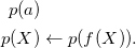
 \begin{align*}{a_{I}} & = a &{a_{\overline{I}}} & = \top \text{ if } a \in I \\& &{a_{\overline{I}}} & = \bot \text{ if } a \notin I \\{{\mathcal{H}}^{\wedge}_{I}} & = {\{ {F_{I}} \mid F \in {\mathcal{H}} \}}^\wedge &{{\mathcal{H}}^{\wedge}_{\overline{I}}} & = {\{ {F_{\overline{I}}} \mid F \in {\mathcal{H}} \}}^\wedge \\{{\mathcal{H}}^{\vee}_{I}} & = {\{ {F_{I}} \mid F \in {\mathcal{H}} \}}^\vee &{{\mathcal{H}}^{\vee}_{\overline{I}}} & = {\{ {F_{\overline{I}}} \mid F \in {\mathcal{H}} \}}^\vee \\{{(F \rightarrow G)}_{I}} & = {F_{\overline{I}}} \rightarrow {G_{I}} &{{(F \rightarrow G)}_{\overline{I}}} & = {F_{I}} \rightarrow {G_{\overline{I}}},\end{align*}
where a is an atom, ${\mathcal{H}}$
a set of formulas, and F and G are formulas.
${\mathcal{H}}$
a set of formulas, and F and G are formulas.
The id-reduct of an ${\mathcal{F}}$
-program P w.r.t. an interpretation I is
${\mathcal{F}}$
-program P w.r.t. an interpretation I is ${P_{I}} = \{ {r_{I}} \mid r \in P \}$
where
${P_{I}} = \{ {r_{I}} \mid r \in P \}$
where ${r_{I}} = {H(r)} \leftarrow {{B(r)}_{I}}$
. As with
${r_{I}} = {H(r)} \leftarrow {{B(r)}_{I}}$
. As with ${r^{I}}$
, the transformation of r into
${r^{I}}$
, the transformation of r into ${r_{I}}$
leaves the head of r unaffected.
${r_{I}}$
leaves the head of r unaffected.
Example 1 Consider the program containing the single rule
 \begin{align*}p & \leftarrow {\neg} {\neg} p.\end{align*}
We get the following reduced programs w.r.t. interpretations $\emptyset$
and
$\emptyset$
and $\{p\}$
:
$\{p\}$
:
 \begin{align*}{\{p \leftarrow {\neg} {\neg} p \}^{\emptyset}}&=\{p \leftarrow \bot\} &{\{p \leftarrow {\neg} {\neg} p \}^{\{p\}}}&=\{p \leftarrow {\neg} \bot\}\\{\{p \leftarrow {\neg} {\neg} p \}_{\emptyset}}&=\{p \leftarrow {\neg} {\neg} p\}\qquad=&{\{p \leftarrow {\neg} {\neg} p \}_{\{p\}}}&=\{p \leftarrow {\neg} {\neg} p\}\end{align*}
Note that both reducts leave the rule’s head intact.
Extending the definition of positive occurrences, we define a formula as (strictly) positive if all its atoms occur (strictly) positively in the formula. We define an ${\mathcal{F}}$
-program as (strictly) positive if all its rule bodies are (strictly) positive.
${\mathcal{F}}$
-program as (strictly) positive if all its rule bodies are (strictly) positive.
For example, the program in Example 1 is positive but not strictly positive because the only body atom p appears in the scope of two antecedents within the rule body ${\neg} {\neg} p$
.
${\neg} {\neg} p$
.
As put forward by van Emden and Kowalski (Reference van Emden and Kowalski1976), we may associate with each program P its one-step provability operator ${{T}_{P}}$
, defined for any interpretation X as
${{T}_{P}}$
, defined for any interpretation X as
 \begin{align*}{{{T}_{P}}(X)} &= \{ {H(r)} \mid r \in P, X \models {B(r)} \}.\end{align*}
Proposition 3 (Truszczyński Reference Truszczyński2012) Let P be a positive ${\mathcal{F}}$
-program.
${\mathcal{F}}$
-program.
Then, the operator ${{T}_{P}}$
is monotone.
${{T}_{P}}$
is monotone.
Fixed points of ${{T}_{P}}$
are models of P guaranteeing that each contained atom is supported by some rule in P; prefixed points of
${{T}_{P}}$
are models of P guaranteeing that each contained atom is supported by some rule in P; prefixed points of ${{T}_{P}}$
correspond to the models of P. According to Theorem 1(a), the
${{T}_{P}}$
correspond to the models of P. According to Theorem 1(a), the ${{T}_{P}}$
operator has a least fixed point for positive
${{T}_{P}}$
operator has a least fixed point for positive ${\mathcal{F}}$
-programs. We refer to this fixed point as the least model of P and write it as
${\mathcal{F}}$
-programs. We refer to this fixed point as the least model of P and write it as ${\mathit{LM}(P)}$
.
${\mathit{LM}(P)}$
.
Observing that the id-reduct replaces all negative occurrences of atoms, any id-reduct ${P_{I}}$
of a program w.r.t. an interpretation I is positive and thus possesses a least model
${P_{I}}$
of a program w.r.t. an interpretation I is positive and thus possesses a least model ${\mathit{LM}({P_{I}})}$
. This gives rise to the following definition of a stable operator (Truszczyński Reference Truszczyński2012): Given an
${\mathit{LM}({P_{I}})}$
. This gives rise to the following definition of a stable operator (Truszczyński Reference Truszczyński2012): Given an ${\mathcal{F}}$
-program P, its id-stable operator is defined for any interpretation I as
${\mathcal{F}}$
-program P, its id-stable operator is defined for any interpretation I as
 \[{{{S}_{P}}(I)} = {\mathit{LM}({P_{I}})}.\]
The fixed points of ${{S}_{P}}$
are the id-stable models of P.
${{S}_{P}}$
are the id-stable models of P.
Note that neither the program reduct ${P^{I}}$
nor the formula reduct
${P^{I}}$
nor the formula reduct ${F^{I}}$
guarantee (least) models. Also, stable models and id-stable models do not coincide in general.
${F^{I}}$
guarantee (least) models. Also, stable models and id-stable models do not coincide in general.
Example 2 Reconsider the program from Example 1, comprising rule
 \begin{align*}p & \leftarrow {\neg} {\neg} p.\end{align*}
This program has the two stable models $\emptyset$
and
$\emptyset$
and $\{p\}$
, but the empty model is the only id-stable model.
$\{p\}$
, but the empty model is the only id-stable model.
Proposition 4 (Truszczyński Reference Truszczyński2012) Let P be an ${\mathcal{F}}$
-program.
${\mathcal{F}}$
-program.
Then, the id-stable operator ${{S}_{P}}$
is antimonotone.
${{S}_{P}}$
is antimonotone.
No analogous antimonotone operator is obtainable for ${\mathcal{F}}$
-programs by using the program reduct
${\mathcal{F}}$
-programs by using the program reduct ${P^{I}}$
(and for general theories with the formula reduct
${P^{I}}$
(and for general theories with the formula reduct ${F^{I}}$
). To see this, reconsider Example 2 along with its two stable models
${F^{I}}$
). To see this, reconsider Example 2 along with its two stable models $\emptyset$
and
$\emptyset$
and $\{p\}$
. Given that both had to be fixed points of such an operator, it would behave monotonically on
$\{p\}$
. Given that both had to be fixed points of such an operator, it would behave monotonically on $\emptyset$
and
$\emptyset$
and $\{p\}$
.
$\{p\}$
.
In view of this, we henceforth consider exclusively id-stable operators and drop the prefix “id”. However, we keep the distinction between stable and id-stable models.
Truszczyński (Reference Truszczyński2012) identifies in a class of programs for which stable models and id-stable models coincide. The set ${\mathcal{N}}$
consists of all formulas F such that any implication in F has
${\mathcal{N}}$
consists of all formulas F such that any implication in F has $\bot$
as consequent and no occurrences of implications in its antecedent. An
$\bot$
as consequent and no occurrences of implications in its antecedent. An ${\mathcal{N}}$
-program consists of rules of form
${\mathcal{N}}$
-program consists of rules of form $ h \leftarrow F $
where
$ h \leftarrow F $
where $h \in {\mathcal{F}}_0$
and
$h \in {\mathcal{F}}_0$
and $F \in {\mathcal{N}}$
.
$F \in {\mathcal{N}}$
.
Proposition 5 (Truszczyński Reference Truszczyński2012) Let P be an ${\mathcal{N}}$
-program.
${\mathcal{N}}$
-program.
Then, the stable and id-stable models of P coincide.
Note that a positive ${\mathcal{N}}$
-program is also strictly positive.
${\mathcal{N}}$
-program is also strictly positive.
2.4 Well-founded models
Our terminology in this section follows the one of Truszczyński (Reference Truszczyński, Kifer and Liu2018) and traces back to the early work of Belnap (Reference Belnap1977) and Fitting (Reference Fitting2002). Footnote 2
We deal with pairs of sets and extend the basic set relations and operations accordingly. Given sets I’, I, J’, J, and X, we define:
-
$(I',J') \mathrel{\bar{\prec}} (I,J)$
if
$I' \prec I$
and
$J' \prec J$
for
$(\bar{\prec}, \prec) \in \{ (\sqsubset, \subset), (\sqsubseteq, \subseteq) \}$
-
$(I',J') \mathrel{\bar{\circ}} (I,J) = (I' \circ I, J' \circ J)$
for
$(\bar{\circ}, \circ) \in \{ (\sqcup, \cup), (\sqcap, \cap), (\smallsetminus,\setminus) \}$
-
$(I,J) \mathrel{\bar{\circ}} X = (I,J) \mathrel{\bar{\circ}} (X,X)$
for
$\bar{\circ} \in \{ \sqcup, \sqcap, \smallsetminus \}$


A four-valued interpretation over signature ${\Sigma}$
is represented by a pair
${\Sigma}$
is represented by a pair $(I,J) \sqsubseteq ({\Sigma}, {\Sigma})$
where I stands for certain and J for possible atoms. Intuitively, an atom that is
$(I,J) \sqsubseteq ({\Sigma}, {\Sigma})$
where I stands for certain and J for possible atoms. Intuitively, an atom that is
-
certain and possible is true,
-
certain but not possible is inconsistent,
-
not certain but possible is unknown, and
-
not certain and not possible is false.
A four-valued interpretation (I’,J’) is more precise than a four-valued interpretation (I,J), written $(I,J) \leq_p (I',J')$
, if
$(I,J) \leq_p (I',J')$
, if $I \subseteq I'$
and
$I \subseteq I'$
and $J' \subseteq J$
. The precision ordering also has an intuitive reading: the more atoms are certain or the fewer atoms are possible, the more precise is an interpretation. The least precise four-valued interpretation over
$J' \subseteq J$
. The precision ordering also has an intuitive reading: the more atoms are certain or the fewer atoms are possible, the more precise is an interpretation. The least precise four-valued interpretation over ${\Sigma}$
is
${\Sigma}$
is $(\emptyset,{\Sigma})$
. As with two-valued interpretations, the set of all four-valued interpretations over a signature
$(\emptyset,{\Sigma})$
. As with two-valued interpretations, the set of all four-valued interpretations over a signature ${\Sigma}$
together with the relation
${\Sigma}$
together with the relation $\leq_p$
forms a complete lattice. A four-valued interpretation is called inconsistent if it contains an inconsistent atom; otherwise, it is called consistent. It is total whenever it makes all atoms either true or false. Finally, (I,J) is called finite whenever both I and J are finite.
$\leq_p$
forms a complete lattice. A four-valued interpretation is called inconsistent if it contains an inconsistent atom; otherwise, it is called consistent. It is total whenever it makes all atoms either true or false. Finally, (I,J) is called finite whenever both I and J are finite.
Following Truszczyński (Reference Truszczyński, Kifer and Liu2018), we define the id-well-founded operator of an ${\mathcal{F}}$
-program P for any four-valued interpretation (I,J) as
${\mathcal{F}}$
-program P for any four-valued interpretation (I,J) as
 \[{{{W}_{P}}(I,J)} = ({{{S}_{P}}(J)}, {{{S}_{P}}(I)}).\]
This operator is monotone w.r.t. the precision ordering $\leq_p$
. Hence, by Theorem 1(b),
$\leq_p$
. Hence, by Theorem 1(b), ${{W}_{P}}$
has a least fixed point, which defines the id-well-founded model of P, also written as
${{W}_{P}}$
has a least fixed point, which defines the id-well-founded model of P, also written as ${\mathit{WM}(P)}$
. In what follows, we drop the prefix “id” and simply refer to the id-well-founded model of a program as its well-founded model. (We keep the distinction between stable and id-stable models.)
${\mathit{WM}(P)}$
. In what follows, we drop the prefix “id” and simply refer to the id-well-founded model of a program as its well-founded model. (We keep the distinction between stable and id-stable models.)
Any well-founded model (I,J) of an ${\mathcal{F}}$
-program P satisfies
${\mathcal{F}}$
-program P satisfies $I \subseteq J$
.
$I \subseteq J$
.
Lemma 6 Let P be an ${\mathcal{F}}$
-Program.
${\mathcal{F}}$
-Program.
Then, the well-founded model ${\mathit{WM}(P)}$
of P is consistent.
${\mathit{WM}(P)}$
of P is consistent.
Example 3 Consider program ${{P}_{3}}$
consisting of the following rules:
${{P}_{3}}$
consisting of the following rules:
 \begin{align*}a & \\b & \leftarrow a \\c & \leftarrow {\neg} b \\d & \leftarrow c \\e & \leftarrow {\neg} d.\end{align*}
We compute the well-founded model of ${{P}_{3}} $
in four iterations starting from
${{P}_{3}} $
in four iterations starting from $(\emptyset,{\Sigma})$
:
$(\emptyset,{\Sigma})$
:
The left and right column reflect the certain and possible atoms computed at each iteration, respectively. We reach a fixed point at Step 4. Accordingly, the well-founded model of ${{P}_{3}}$
is
${{P}_{3}}$
is $(\{a, b, e\}, \{a, b, e\})$
.
$(\{a, b, e\}, \{a, b, e\})$
.
Unlike general ${\mathcal{F}}$
-programs, the class of
${\mathcal{F}}$
-programs, the class of ${\mathcal{N}}$
-programs warrants the same stable and id-stable models for each of its programs. Unfortunately,
${\mathcal{N}}$
-programs warrants the same stable and id-stable models for each of its programs. Unfortunately, ${\mathcal{N}}$
-programs are too restricted for our purpose (for instance, for capturing aggregates in rule bodies
Footnote 3
). To this end, we define a more general class of programs and refer to them as
${\mathcal{N}}$
-programs are too restricted for our purpose (for instance, for capturing aggregates in rule bodies
Footnote 3
). To this end, we define a more general class of programs and refer to them as ${\mathcal{R}}$
-programs. Although id-stable models of
${\mathcal{R}}$
-programs. Although id-stable models of ${\mathcal{R}}$
-programs may differ from their stable models (see below), their well-founded models encompass both stable and id-stable models. Thus, well-founded models can be used for characterizing stable model-preserving program transformations. In fact, we see in Section 2.5 that the restriction of
${\mathcal{R}}$
-programs may differ from their stable models (see below), their well-founded models encompass both stable and id-stable models. Thus, well-founded models can be used for characterizing stable model-preserving program transformations. In fact, we see in Section 2.5 that the restriction of ${\mathcal{F}}$
- to
${\mathcal{F}}$
- to ${\mathcal{R}}$
-programs allows us to provide tighter semantic characterizations of program simplifications.e define
${\mathcal{R}}$
-programs allows us to provide tighter semantic characterizations of program simplifications.e define ${\mathcal{R}}$
to be the set of all formulas F such that implications in F have no further occurrences of implications in their antecedents. Then, an
${\mathcal{R}}$
to be the set of all formulas F such that implications in F have no further occurrences of implications in their antecedents. Then, an ${\mathcal{R}}$
-program consists of rules of form
${\mathcal{R}}$
-program consists of rules of form $h \leftarrow F$
where
$h \leftarrow F$
where $h \in {\mathcal{F}}_0$
and
$h \in {\mathcal{F}}_0$
and $F \in {\mathcal{R}}$
. As with
$F \in {\mathcal{R}}$
. As with ${\mathcal{N}}$
-programs, a positive
${\mathcal{N}}$
-programs, a positive ${\mathcal{R}}$
-program is also strictly positive.
${\mathcal{R}}$
-program is also strictly positive.
Our next result shows that (id-)well-founded models can be used for approximating (regular) stable models of ${\mathcal{R}}$
-programs.
${\mathcal{R}}$
-programs.
Theorem 7 Let P be an ${\mathcal{R}}$
-program and (I,J) be the well-founded model of P.
${\mathcal{R}}$
-program and (I,J) be the well-founded model of P.
If X is a stable model of P, then $I \subseteq X \subseteq J$
.
$I \subseteq X \subseteq J$
.
Example 4 Consider the ${\mathcal{R}}$
-program
${\mathcal{R}}$
-program ${{P}_{4}}$
:
Footnote 4
${{P}_{4}}$
:
Footnote 4
 \begin{align*}c & \leftarrow (b \rightarrow a) &a & \leftarrow b \\a & \leftarrow c &b & \leftarrow a.\end{align*}
Observe that $\{a, b, c\}$
is the only stable model of
$\{a, b, c\}$
is the only stable model of ${{P}_{4}}$
, the program does not have any id-stable models, and the well-founded model of
${{P}_{4}}$
, the program does not have any id-stable models, and the well-founded model of ${{P}_{4}}$
is
${{P}_{4}}$
is $(\emptyset,\{a,b,c\})$
. In accordance with Theorem 7, the stable model of
$(\emptyset,\{a,b,c\})$
. In accordance with Theorem 7, the stable model of ${{P}_{4}}$
is enclosed in the well-founded model.
${{P}_{4}}$
is enclosed in the well-founded model.
Note that the id-reduct handles $b \rightarrow a$
the same way as
$b \rightarrow a$
the same way as ${\neg} b \vee a$
. In fact, the program obtained by replacing
${\neg} b \vee a$
. In fact, the program obtained by replacing
 \begin{align*}c & \leftarrow (b \rightarrow a)\end{align*}
with
 \begin{align*}c & \leftarrow {\neg} b \vee a\end{align*}
is an ${\mathcal{N}}$
-program and has neither stable nor id-stable models.
${\mathcal{N}}$
-program and has neither stable nor id-stable models.
Further, note that the program in Example 2 is not an ${\mathcal{R}}$
-program, whereas the one in Example 3 is an
${\mathcal{R}}$
-program, whereas the one in Example 3 is an ${\mathcal{R}}$
-program.
${\mathcal{R}}$
-program.
2.5 Program simplification
In this section, we define a concept of program simplification relative to a four-valued interpretation and show how its result can be characterized by the semantic means from above. This concept has two important properties. First, it results in a finite program whenever the interpretation used for simplification is finite. And second, it preserves all (regular) stable models of ${\mathcal{R}}$
-programs when simplified with their well-founded models.
${\mathcal{R}}$
-programs when simplified with their well-founded models.
Definition 1 Let P be an ${\mathcal{F}}$
-program, and (I,J) be a four-valued interpretation.
${\mathcal{F}}$
-program, and (I,J) be a four-valued interpretation.
We define the simplification of P w.r.t. (I,J) as
 \begin{align*}{P^{(I,J)}} & = \{ r \in P \mid J \models {{B(r)}_{I}} \}.\end{align*}
For simplicity, we drop parentheses and we write ${P^{I,J}}$
instead of
${P^{I,J}}$
instead of ${P^{(I,J)}}$
whenever clear from context.
${P^{(I,J)}}$
whenever clear from context.
The program simplification ${P^{I,J}}$
acts as a filter eliminating inapplicable rules that fail to satisfy the condition
${P^{I,J}}$
acts as a filter eliminating inapplicable rules that fail to satisfy the condition $J \models {{B(r)}_{I}}$
. That is, first, all negatively occurring atoms in B(r) are evaluated w.r.t. the certain atoms in I and replaced accordingly by
$J \models {{B(r)}_{I}}$
. That is, first, all negatively occurring atoms in B(r) are evaluated w.r.t. the certain atoms in I and replaced accordingly by $\bot$
and
$\bot$
and $\top$
, respectively. Then, it is checked whether the reduced body
$\top$
, respectively. Then, it is checked whether the reduced body ${{B(r)}_{I}}$
is satisfiable by the possible atoms in J. Only in this case, the rule is kept in
${{B(r)}_{I}}$
is satisfiable by the possible atoms in J. Only in this case, the rule is kept in $P^{I,J}$
. No simplifications are applied to the remaining rules. This is illustrated in Example 5 below.
$P^{I,J}$
. No simplifications are applied to the remaining rules. This is illustrated in Example 5 below.
Note that ${P^{I,J}}$
is finite whenever (I,J) is finite.
${P^{I,J}}$
is finite whenever (I,J) is finite.
Observe that for an ${\mathcal{F}}$
-program P the head atoms in
${\mathcal{F}}$
-program P the head atoms in ${{P^{I,J}}}$
correspond to the result of applying the provability operator of program
${{P^{I,J}}}$
correspond to the result of applying the provability operator of program ${P_{I}}$
to the possible atoms in J, that is,
${P_{I}}$
to the possible atoms in J, that is, ${H({P^{I,J}})} = {{{T}_{{P_{I}}}}(J)}$
.
${H({P^{I,J}})} = {{{T}_{{P_{I}}}}(J)}$
.
Our next result shows that programs simplified with their well-founded model maintain this model.
Theorem 8 Let P be an ${\mathcal{F}}$
-program and (I,J) be the well-founded model of P.
${\mathcal{F}}$
-program and (I,J) be the well-founded model of P.
Then, P and ${P^{I,J}}$
have the same well-founded model.
${P^{I,J}}$
have the same well-founded model.
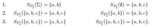
Example 5 In Example 3, we computed the well-founded model $(\{a, b, e\}, \{a, b, e\})$
of
$(\{a, b, e\}, \{a, b, e\})$
of ${{P}_{3}}$
. With this, we obtain the simplified program
${{P}_{3}}$
. With this, we obtain the simplified program ${{P}_{3}'} = {{{P}_{3}}^{\{a, b, e\}, \{a, b, e\}}}$
after dropping
${{P}_{3}'} = {{{P}_{3}}^{\{a, b, e\}, \{a, b, e\}}}$
after dropping $c \leftarrow {\neg} b$
and
$c \leftarrow {\neg} b$
and $d \leftarrow c$
:
$d \leftarrow c$
:
 \begin{align*}a & \\b & \leftarrow a \\e & \leftarrow {\neg} d.\end{align*}
Next, we check that the well-founded model of ${{P}_{3}'}$
corresponds to the well-founded model of
${{P}_{3}'}$
corresponds to the well-founded model of ${{P}_{3}}$
:
${{P}_{3}}$
:
We observe that it takes two applications of the well-founded operator to obtain the well-founded model. This could be reduced to one step if atoms false in the well-founded model would be removed from the negative bodies by the program simplification. Keeping them is a design decision with the goal to simplify notation in the following.
The next series of results further elaborates on semantic invariants guaranteed by our concept of program simplification. The first result shows that it preserves all stable models between the sets used for simplification.
Theorem 9 Let P be an ${\mathcal{F}}$
-program, and I, J, and X be two-valued interpretations.
${\mathcal{F}}$
-program, and I, J, and X be two-valued interpretations.
If $I \subseteq X \subseteq J$
, then X is a stable model of P iff X is a stable model of
$I \subseteq X \subseteq J$
, then X is a stable model of P iff X is a stable model of ${P^{I,J}}$
.
${P^{I,J}}$
.
As a consequence, we obtain that ${\mathcal{R}}$
-programs simplified with their well-founded model also maintain stable models.
${\mathcal{R}}$
-programs simplified with their well-founded model also maintain stable models.
Corollary 10 Let P be an ${\mathcal{R}}$
-program and (I,J) be the well-founded model of P.
${\mathcal{R}}$
-program and (I,J) be the well-founded model of P.
Then, P and ${P^{I,J}}$
have the same stable models.
${P^{I,J}}$
have the same stable models.
For instance, the ${\mathcal{R}}$
-program in Example 3 and its simplification in Example 5 have the same stable model. Unlike this, the program from Example 2 consisting of rule
${\mathcal{R}}$
-program in Example 3 and its simplification in Example 5 have the same stable model. Unlike this, the program from Example 2 consisting of rule $p \leftarrow {\neg} {\neg} p$
induces two stable models, while its simplification w.r.t. its well-founded model
$p \leftarrow {\neg} {\neg} p$
induces two stable models, while its simplification w.r.t. its well-founded model $(\emptyset,\emptyset)$
yields an empty program admitting the empty stable model only.
$(\emptyset,\emptyset)$
yields an empty program admitting the empty stable model only.
Note that given an ${\mathcal{R}}$
-program with a finite well-founded model, we obtain a semantically equivalent finite program via simplification. As detailed in the following sections, grounding algorithms only compute approximations of the well-founded model. However, as long as the approximation is finite, we still obtain semantically equivalent finite programs. This is made precise by the next two results showing that any program between the original and its simplification relative to its well-founded model preserves the well-founded model, and that this extends to all stable models for
${\mathcal{R}}$
-program with a finite well-founded model, we obtain a semantically equivalent finite program via simplification. As detailed in the following sections, grounding algorithms only compute approximations of the well-founded model. However, as long as the approximation is finite, we still obtain semantically equivalent finite programs. This is made precise by the next two results showing that any program between the original and its simplification relative to its well-founded model preserves the well-founded model, and that this extends to all stable models for ${\mathcal{R}}$
-programs.
${\mathcal{R}}$
-programs.
Theorem 11 Let P and Q be ${\mathcal{F}}$
-programs, and (I,J) be the well-founded model of P.
${\mathcal{F}}$
-programs, and (I,J) be the well-founded model of P.
If ${P^{I,J}} \subseteq Q \subseteq P$
, then P and Q have the same well-founded models.
${P^{I,J}} \subseteq Q \subseteq P$
, then P and Q have the same well-founded models.
Corollary 12 Let P and Q be ${\mathcal{R}}$
-programs, and (I,J) be the well-founded model of P.
${\mathcal{R}}$
-programs, and (I,J) be the well-founded model of P.
If ${P^{I,J}} \subseteq Q \subseteq P$
, then P and Q are equivalent.
${P^{I,J}} \subseteq Q \subseteq P$
, then P and Q are equivalent.
3 Splitting
One of the first steps during grounding is to group rules into components suitable for successive instantiation. This amounts to splitting a logic program into a sequence of subprograms. The rules in each such component are then instantiated with respect to the atoms possibly derivable from previous components, starting with some component consisting of facts only. In other words, grounding is always performed relative to a set of atoms that provide a context. Moreover, atoms found to be true or false can be used for on-the-fly simplifications.
Accordingly, this section parallels the above presentation by extending the respective formal concepts with contextual information provided by atoms in a two- and four-valued setting. We then assemble the resulting concepts to enable their consecutive application to sequences of subprograms. Interestingly, the resulting notion of splitting allows for more fine-grained splitting than the traditional concept (Lifschitz and Turner Reference Lifschitz and Turner1994) since it allows us to partition rules in an arbitrary way. In view of grounding, we show that once a program is split into a sequence of programs, we can iteratively compute an approximation of the well-founded model by considering in turn each element in the sequence.
In what follows, we append letter “C” to names of interpretations having a contextual nature.
To begin with, we extend the one-step provability operator accordingly.
Definition 2 Let P be an ${\mathcal{F}}$
-program and
${\mathcal{F}}$
-program and ${\mathit{I\!{C}}}$
be a two-valued interpretation.
${\mathit{I\!{C}}}$
be a two-valued interpretation.
For any two-valued interpretation I, we define the one-step provability operator of P relative to ${\mathit{I\!{C}}}$
as
${\mathit{I\!{C}}}$
as
 \begin{align*}{{{T}_{P}^{{\mathit{I\!{C}}}}}(I)} &= {{{T}_{P}}({\mathit{I\!{C}}} \cup I)}.\end{align*}
A prefixed point of ${{T}_{P}^{{\mathit{I\!{C}}}}}$
is a also a prefixed point of
${{T}_{P}^{{\mathit{I\!{C}}}}}$
is a also a prefixed point of ${{T}_{P}}$
. Thus, each prefixed point of
${{T}_{P}}$
. Thus, each prefixed point of ${{T}_{P}^{{\mathit{I\!{C}}}}}$
is a model of P but not vice versa.
${{T}_{P}^{{\mathit{I\!{C}}}}}$
is a model of P but not vice versa.
To see this, consider program $P=\{a \leftarrow b\}$
. We have
$P=\{a \leftarrow b\}$
. We have ${{{T}_{P}}(\emptyset)} = \emptyset$
and
${{{T}_{P}}(\emptyset)} = \emptyset$
and ${{{T}_{P}^{\{b\}}}(\emptyset)} = \{a\}$
. Hence,
${{{T}_{P}^{\{b\}}}(\emptyset)} = \{a\}$
. Hence, $\emptyset$
is a (pre)fixed point of
$\emptyset$
is a (pre)fixed point of ${{T}_{P}}$
but not of
${{T}_{P}}$
but not of ${{T}_{P}^{\{b\}}}$
since
${{T}_{P}^{\{b\}}}$
since $\{a\} \not\subseteq \emptyset$
. The set
$\{a\} \not\subseteq \emptyset$
. The set $\{a\}$
is a prefixed point of both operators.
$\{a\}$
is a prefixed point of both operators.
Proposition 13 Let P be a positive program, and ${\mathit{I\!{C}}}$
and J be two valued interpretations.
${\mathit{I\!{C}}}$
and J be two valued interpretations.
Then, the operators ${{T}_{P}^{{\mathit{I\!{C}}}}}$
and
${{T}_{P}^{{\mathit{I\!{C}}}}}$
and ${{{T}_{P}^{\,\boldsymbol{\cdot}}}(J)}$
are both monotone.
${{{T}_{P}^{\,\boldsymbol{\cdot}}}(J)}$
are both monotone.
We use Theorems 1 and 13 to define a contextual stable operator.
Definition 3 Let P be an ${\mathcal{F}}$
-program and
${\mathcal{F}}$
-program and ${\mathit{I\!{C}}}$
be a two-valued interpretation.
${\mathit{I\!{C}}}$
be a two-valued interpretation.
For any two-valued interpretation J, we define the stable operator relative to ${\mathit{I\!{C}}}$
, written
${\mathit{I\!{C}}}$
, written ${{{S}_{P}^{{\mathit{I\!{C}}}}}(J)}$
, as the least fixed point of
${{{S}_{P}^{{\mathit{I\!{C}}}}}(J)}$
, as the least fixed point of ${{T}_{{P_{J}}}^{{\mathit{I\!{C}}}}}$
.
${{T}_{{P_{J}}}^{{\mathit{I\!{C}}}}}$
.
While the operator is antimonotone w.r.t. its argument J, it is monotone regarding its parameter ${\mathit{I\!{C}}}$
.
${\mathit{I\!{C}}}$
.
Proposition 14 Let P be an ${\mathcal{F}}$
-program, and
${\mathcal{F}}$
-program, and ${\mathit{I\!{C}}}$
and J be two-valued interpretations.
${\mathit{I\!{C}}}$
and J be two-valued interpretations.
Then, the operators ${{S}_{P}^{{\mathit{I\!{C}}}}}$
and
${{S}_{P}^{{\mathit{I\!{C}}}}}$
and ${{{S}_{P}^{\,\boldsymbol{\cdot}}}(J)}$
are antimonotone and monotone, respectively.
${{{S}_{P}^{\,\boldsymbol{\cdot}}}(J)}$
are antimonotone and monotone, respectively.
By building on the relative stable operator, we next define its well-founded counterpart. Unlike above, the context is now captured by a four-valued interpretation.
Definition 4 Let P be an ${\mathcal{F}}$
-program and
${\mathcal{F}}$
-program and $({\mathit{I\!{C}}},{\mathit{J\!{C}}})$
be a four-valued interpretation.
$({\mathit{I\!{C}}},{\mathit{J\!{C}}})$
be a four-valued interpretation.
For any four-valued interpretation (I,J), we define the well-founded operator relative to $({\mathit{I\!{C}}},{\mathit{J\!{C}}})$
as
$({\mathit{I\!{C}}},{\mathit{J\!{C}}})$
as
 \begin{align*}{{{W}_{P}^{({\mathit{I\!{C}}},{\mathit{J\!{C}}})}}(I,J)} = ({{{S}_{P}^{{\mathit{I\!{C}}}}}(J \cup {\mathit{J\!{C}}})}, {{{S}_{P}^{{\mathit{J\!{C}}}}}(I \cup {\mathit{I\!{C}}})}).\end{align*}
As above, we drop parentheses and simply write ${{W}_{P}^{I,J}}$
instead of
${{W}_{P}^{I,J}}$
instead of ${{W}_{P}^{(I,J)}}$
. Also, we keep refraining from prepending the prefix “id” to the well-founded operator along with all concepts derived from it below.
${{W}_{P}^{(I,J)}}$
. Also, we keep refraining from prepending the prefix “id” to the well-founded operator along with all concepts derived from it below.
Unlike the stable operator, the relative well-founded one is monotone on both its argument and parameter.
Proposition 15 Let P be an ${\mathcal{F}}$
-program, and (I,J) and
${\mathcal{F}}$
-program, and (I,J) and $({\mathit{I\!{C}}},{\mathit{J\!{C}}})$
be four-valued interpretations.
$({\mathit{I\!{C}}},{\mathit{J\!{C}}})$
be four-valued interpretations.
Then, the operators ${{W}_{P}^{{\mathit{I\!{C}}},{\mathit{J\!{C}}}}}$
and
${{W}_{P}^{{\mathit{I\!{C}}},{\mathit{J\!{C}}}}}$
and ${{{W}_{P}^{\,\boldsymbol{\cdot}}}(I,J)}$
are both monotone w.r.t. the precision ordering.
${{{W}_{P}^{\,\boldsymbol{\cdot}}}(I,J)}$
are both monotone w.r.t. the precision ordering.
From Theorems 1 and 15, we get that the relative well-founded operator has a least fixed point.
Definition 5 Let P be an ${\mathcal{F}}$
-program and
${\mathcal{F}}$
-program and $({\mathit{I\!{C}}},{\mathit{J\!{C}}})$
be a four-valued interpretation.
$({\mathit{I\!{C}}},{\mathit{J\!{C}}})$
be a four-valued interpretation.
We define the well-founded model of P relative to $({\mathit{I\!{C}}},{\mathit{J\!{C}}})$
, written
$({\mathit{I\!{C}}},{\mathit{J\!{C}}})$
, written ${\mathit{WM}^{({\mathit{I\!{C}}},{\mathit{J\!{C}}})}(P)}$
, as the least fixed point of
${\mathit{WM}^{({\mathit{I\!{C}}},{\mathit{J\!{C}}})}(P)}$
, as the least fixed point of ${{W}_{P}^{{\mathit{I\!{C}}},{\mathit{J\!{C}}}}}$
.
${{W}_{P}^{{\mathit{I\!{C}}},{\mathit{J\!{C}}}}}$
.
Whenever clear from context, we keep dropping parentheses and simply write ${\mathit{WM}^{I,J}(P)}$
instead of
${\mathit{WM}^{I,J}(P)}$
instead of ${\mathit{WM}^{(I,J)}(P)}$
.
${\mathit{WM}^{(I,J)}(P)}$
.
In what follows, we use the relativized concepts defined above to delineate the semantics and resulting simplifications of the sequence of subprograms resulting from a grounder’s decomposition of the original program. For simplicity, we first present a theorem capturing the composition under the well-founded operation, before we give the general case involving a sequence of programs.
Just like suffix C, we use the suffix E (and similarly letter E further below) to indicate atoms whose defining rules are yet to come.
As in traditional splitting, we begin by differentiating a bottom and a top program. In addition to the input atoms (I,J) and context atoms in $({\mathit{I\!{C}}},{\mathit{J\!{C}}})$
, we moreover distinguish a set of external atoms,
$({\mathit{I\!{C}}},{\mathit{J\!{C}}})$
, we moreover distinguish a set of external atoms, $({\mathit{I\!{E}}},{\mathit{J\!{E}}})$
, which occur in the bottom program but are defined in the top program. Accordingly, the bottom program has to be evaluated relative to
$({\mathit{I\!{E}}},{\mathit{J\!{E}}})$
, which occur in the bottom program but are defined in the top program. Accordingly, the bottom program has to be evaluated relative to $({\mathit{I\!{C}}},{\mathit{J\!{C}}}) \sqcup ({\mathit{I\!{E}}},{\mathit{J\!{E}}})$
(and not just
$({\mathit{I\!{C}}},{\mathit{J\!{C}}}) \sqcup ({\mathit{I\!{E}}},{\mathit{J\!{E}}})$
(and not just $({\mathit{I\!{C}}},{\mathit{J\!{C}}})$
as above) to consider what could be derived by the top program. Also, observe that our notion of splitting aims at computing well-founded models rather than stable models.
$({\mathit{I\!{C}}},{\mathit{J\!{C}}})$
as above) to consider what could be derived by the top program. Also, observe that our notion of splitting aims at computing well-founded models rather than stable models.
Theorem 16 Let ${\mathit{P\!{B}}}$
and
${\mathit{P\!{B}}}$
and ${\mathit{P\!{T}}}$
be
${\mathit{P\!{T}}}$
be ${\mathcal{F}}$
-programs,
${\mathcal{F}}$
-programs, $({\mathit{I\!{C}}},{\mathit{J\!{C}}})$
be a four-valued interpretation,
$({\mathit{I\!{C}}},{\mathit{J\!{C}}})$
be a four-valued interpretation, $(I,J) = {\mathit{WM}^{{\mathit{I\!{C}}},{\mathit{J\!{C}}}}({\mathit{P\!{B}}} \cup {\mathit{P\!{T}}})}$
,
$(I,J) = {\mathit{WM}^{{\mathit{I\!{C}}},{\mathit{J\!{C}}}}({\mathit{P\!{B}}} \cup {\mathit{P\!{T}}})}$
, $({\mathit{I\!{E}}},{\mathit{J\!{E}}}) = (I, J) \sqcap ({{{B({\mathit{P\!{B}}})}}^\pm} \cap {H({\mathit{P\!{T}}})})$
,
$({\mathit{I\!{E}}},{\mathit{J\!{E}}}) = (I, J) \sqcap ({{{B({\mathit{P\!{B}}})}}^\pm} \cap {H({\mathit{P\!{T}}})})$
, $({\mathit{I\!{B}}},{\mathit{J\!{B}}}) = {\mathit{WM}^{({\mathit{I\!{C}}}, {\mathit{J\!{C}}}) \sqcup ({\mathit{I\!{E}}},{\mathit{J\!{E}}})}({\mathit{P\!{B}}})}$
, and
$({\mathit{I\!{B}}},{\mathit{J\!{B}}}) = {\mathit{WM}^{({\mathit{I\!{C}}}, {\mathit{J\!{C}}}) \sqcup ({\mathit{I\!{E}}},{\mathit{J\!{E}}})}({\mathit{P\!{B}}})}$
, and $({{\mathit{I\!{T}}}},{{\mathit{J\!{T}}}}) = {\mathit{WM}^{({\mathit{I\!{C}}}, {\mathit{J\!{C}}}) \sqcup ({\mathit{I\!{B}}},{\mathit{J\!{B}}})}({\mathit{P\!{T}}})}$
.
$({{\mathit{I\!{T}}}},{{\mathit{J\!{T}}}}) = {\mathit{WM}^{({\mathit{I\!{C}}}, {\mathit{J\!{C}}}) \sqcup ({\mathit{I\!{B}}},{\mathit{J\!{B}}})}({\mathit{P\!{T}}})}$
.
Then, we have $(I,J) = ({\mathit{I\!{B}}},{\mathit{J\!{B}}}) \sqcup ({{\mathit{I\!{T}}}},{{\mathit{J\!{T}}}})$
.
$(I,J) = ({\mathit{I\!{B}}},{\mathit{J\!{B}}}) \sqcup ({{\mathit{I\!{T}}}},{{\mathit{J\!{T}}}})$
.
Partially expanding the statements of the two previous result nicely reflects the decomposition of the application of the well-founded founded model of a program:
 \begin{align*}{\mathit{WM}^{{\mathit{I\!{C}}},{\mathit{J\!{C}}}}({\mathit{P\!{B}}} \cup {\mathit{P\!{T}}})} &= {\mathit{WM}^{({\mathit{I\!{C}}}, {\mathit{J\!{C}}}) \sqcup ({\mathit{I\!{E}}},{\mathit{J\!{E}}})}({\mathit{P\!{B}}})} \sqcup {\mathit{WM}^{({\mathit{I\!{C}}}, {\mathit{J\!{C}}}) \sqcup ({\mathit{I\!{B}}},{\mathit{J\!{B}}})}({\mathit{P\!{T}}})}.\end{align*}
Note that the formulation of the theorem forms the external interpretation $({\mathit{I\!{E}}},{\mathit{J\!{E}}})$
, by selecting atoms from the overarching well-founded model (I,J). This warrants the correspondence of the overall interpretations to the union of the bottom and top well-founded model. This global approach is dropped below (after the next example) and leads to less precise composed models.
$({\mathit{I\!{E}}},{\mathit{J\!{E}}})$
, by selecting atoms from the overarching well-founded model (I,J). This warrants the correspondence of the overall interpretations to the union of the bottom and top well-founded model. This global approach is dropped below (after the next example) and leads to less precise composed models.
Example 6 Let us illustrate the above approach via the following program:
 \begin{align}a &\end{align}
 \begin{align}b &\end{align}
 \begin{align}c & \leftarrow a\end{align}
 \begin{align}d & \leftarrow {\neg} b.\end{align}
The well-founded model of this program relative to $({\mathit{I\!{C}}},{\mathit{J\!{C}}})=(\emptyset, \emptyset)$
is
$({\mathit{I\!{C}}},{\mathit{J\!{C}}})=(\emptyset, \emptyset)$
is
 \[(I,J) = (\{a,b,c\},\{a,b,c\}).\]
First, we partition the four rules of the program into ${\mathit{P\!{B}}}$
and
${\mathit{P\!{B}}}$
and ${\mathit{P\!{T}}}$
as given above. We get
${\mathit{P\!{T}}}$
as given above. We get $({\mathit{I\!{E}}},{\mathit{J\!{E}}})= (\emptyset,\emptyset)$
since
$({\mathit{I\!{E}}},{\mathit{J\!{E}}})= (\emptyset,\emptyset)$
since ${{{B({\mathit{P\!{B}}})}}^\pm} \cap {H({\mathit{P\!{T}}})}=\emptyset$
. Let us evaluate
${{{B({\mathit{P\!{B}}})}}^\pm} \cap {H({\mathit{P\!{T}}})}=\emptyset$
. Let us evaluate ${\mathit{P\!{B}}}$
before
${\mathit{P\!{B}}}$
before ${\mathit{P\!{T}}}$
. The well-founded model of
${\mathit{P\!{T}}}$
. The well-founded model of ${\mathit{P\!{B}}}$
relative to
${\mathit{P\!{B}}}$
relative to $({\mathit{I\!{C}}},{\mathit{J\!{C}}}) \sqcup ({\mathit{I\!{E}}},{\mathit{J\!{E}}})$
is
$({\mathit{I\!{C}}},{\mathit{J\!{C}}}) \sqcup ({\mathit{I\!{E}}},{\mathit{J\!{E}}})$
is
 \[({\mathit{I\!{B}}},{\mathit{J\!{B}}}) = (\{a,b\},\{a,b\}).\]
With this, we calculate the well-founded model of ${\mathit{P\!{T}}}$
relative to
${\mathit{P\!{T}}}$
relative to $({\mathit{I\!{C}}},{\mathit{J\!{C}}}) \sqcup ({\mathit{I\!{B}}},{\mathit{J\!{B}}})$
:
$({\mathit{I\!{C}}},{\mathit{J\!{C}}}) \sqcup ({\mathit{I\!{B}}},{\mathit{J\!{B}}})$
:
 \[({\mathit{I\!{T}}},{\mathit{J\!{T}}}) = (\{c\},\{c\}).\]
We see that the union of $({\mathit{I\!{B}}},{\mathit{J\!{B}}}) \sqcup ({\mathit{I\!{T}}},{\mathit{J\!{T}}})$
is the same as the well-founded model of
$({\mathit{I\!{B}}},{\mathit{J\!{B}}}) \sqcup ({\mathit{I\!{T}}},{\mathit{J\!{T}}})$
is the same as the well-founded model of ${\mathit{P\!{B}}} \cup {\mathit{P\!{T}}}$
relative to
${\mathit{P\!{B}}} \cup {\mathit{P\!{T}}}$
relative to $({\mathit{I\!{C}}},{\mathit{J\!{C}}})$
.
$({\mathit{I\!{C}}},{\mathit{J\!{C}}})$
.
This corresponds to standard splitting in the sense that $\{a,b\}$
is a splitting set for
$\{a,b\}$
is a splitting set for ${\mathit{P\!{B}}}\cup {\mathit{P\!{T}}}$
and
${\mathit{P\!{B}}}\cup {\mathit{P\!{T}}}$
and ${\mathit{P\!{B}}}$
is the “bottom” and
${\mathit{P\!{B}}}$
is the “bottom” and ${\mathit{P\!{T}}}$
is the “top” (Lifschitz and Turner Reference Lifschitz and Turner1994).
${\mathit{P\!{T}}}$
is the “top” (Lifschitz and Turner Reference Lifschitz and Turner1994).
Example 7 For a complement, let us reverse the roles of programs ${\mathit{P\!{B}}}$
and
${\mathit{P\!{B}}}$
and ${\mathit{P\!{T}}}$
in Example 6. Unlike above, body atoms in
${\mathit{P\!{T}}}$
in Example 6. Unlike above, body atoms in ${\mathit{P\!{B}}}$
now occur in rule heads of
${\mathit{P\!{B}}}$
now occur in rule heads of ${\mathit{P\!{T}}}$
, that is,
${\mathit{P\!{T}}}$
, that is, ${{{B({\mathit{P\!{B}}})}}^\pm} \cap {{H({\mathit{P\!{T}}})}} = \{a,b\}$
. We thus get
${{{B({\mathit{P\!{B}}})}}^\pm} \cap {{H({\mathit{P\!{T}}})}} = \{a,b\}$
. We thus get $({\mathit{I\!{E}}},{\mathit{J\!{E}}})= (\{a,b\}, \{a, b\})$
. The well-founded model of
$({\mathit{I\!{E}}},{\mathit{J\!{E}}})= (\{a,b\}, \{a, b\})$
. The well-founded model of ${\mathit{P\!{B}}}$
relative to
${\mathit{P\!{B}}}$
relative to $({\mathit{I\!{C}}},{\mathit{J\!{C}}}) \sqcup ({\mathit{I\!{E}}},{\mathit{J\!{E}}})$
is
$({\mathit{I\!{C}}},{\mathit{J\!{C}}}) \sqcup ({\mathit{I\!{E}}},{\mathit{J\!{E}}})$
is
 \begin{align*}({\mathit{I\!{B}}},{\mathit{J\!{B}}}) & = (\{c\}, \{c\}).\end{align*}
And the well-founded model of ${\mathit{P\!{T}}}$
relative to
${\mathit{P\!{T}}}$
relative to $({\mathit{I\!{C}}},{\mathit{J\!{C}}}) \sqcup ({\mathit{I\!{B}}},{\mathit{J\!{B}}})$
is
$({\mathit{I\!{C}}},{\mathit{J\!{C}}}) \sqcup ({\mathit{I\!{B}}},{\mathit{J\!{B}}})$
is
 \begin{align*}({\mathit{I\!{T}}},{\mathit{J\!{T}}}) & = (\{a,b\}, \{a,b\}).\end{align*}
Again, we see that the union of both models is identical to (I,J).
This decomposition has no direct correspondence to standard splitting (Lifschitz and Turner Reference Lifschitz and Turner1994) since there is no splitting set.
Next, we generalize the previous results from two programs to sequences of programs. For this, we let $\mathbb{I}$
be a well-ordered index set and direct our attention to sequences
$\mathbb{I}$
be a well-ordered index set and direct our attention to sequences ${({{P}_{i}})}_{i \in \mathbb{I}}$
of
${({{P}_{i}})}_{i \in \mathbb{I}}$
of ${\mathcal{F}}$
-programs.
${\mathcal{F}}$
-programs.
Definition 6 Let ${({{P}_{i}})}_{i \in \mathbb{I}}$
be a sequence of
${({{P}_{i}})}_{i \in \mathbb{I}}$
be a sequence of ${\mathcal{F}}$
-programs.
${\mathcal{F}}$
-programs.
We define the well-founded model of ${({{P}_{i}})}_{i \in \mathbb{I}}$
as
${({{P}_{i}})}_{i \in \mathbb{I}}$
as
 \begin{align}{\mathit{WM}({({{P}_{i}})}_{i \in \mathbb{I}})} & = \bigsqcup_{i \in \mathbb{I}} ({I_{i}},{J_{i}}),\end{align}
where
 \begin{align}{E_{i}} & = {{{B({{P}_{i}})}}^\pm} \cap \bigcup_{i < j} {H({{P}_{j}})},\end{align}
 \begin{align}({{\mathit{I\!{C}}}_{i}},{{\mathit{J\!{C}}}_{i}}) & = \bigsqcup_{j < i} ({I_{j}},{J_{j}})\text{, and}\end{align}
 \begin{align}({I_{i}},{J_{i}}) & = {\mathit{WM}^{({{\mathit{I\!{C}}}_{i}},{{\mathit{J\!{C}}}_{i}}) \sqcup (\emptyset,{E_{i}})}({{P}_{i}})}.\end{align}
The well-founded model of a program sequence is itself assembled in (2) from a sequence of well-founded models of the individual subprograms in (5). This provides us with semantic guidance for successive program simplification, as shown below. In fact, proceeding along the sequence of subprograms reflects the iterative approach of a grounding algorithm, one component is grounded at a time. At each stage $i \in \mathbb{I}$
, this takes into account the truth values of atoms instantiated in previous iterations, viz.
$i \in \mathbb{I}$
, this takes into account the truth values of atoms instantiated in previous iterations, viz. $({{\mathit{I\!{C}}}_{i}},{{\mathit{J\!{C}}}_{i}})$
, as well as dependencies to upcoming components in
$({{\mathit{I\!{C}}}_{i}},{{\mathit{J\!{C}}}_{i}})$
, as well as dependencies to upcoming components in ${E_{i}}$
. Note that unlike Proposition 16, the external atoms in
${E_{i}}$
. Note that unlike Proposition 16, the external atoms in ${E_{i}}$
are identified purely syntactically, and the interpretation
${E_{i}}$
are identified purely syntactically, and the interpretation $(\emptyset,{E_{i}})$
treats them as unknown. Grounding is thus performed under incomplete information and each well-founded model in (5) can be regarded as an over-approximation of the actual one. This is enabled by the monotonicity of the well-founded operator in Proposition 15 that only leads to a less precise result when overestimating its parameter.
$(\emptyset,{E_{i}})$
treats them as unknown. Grounding is thus performed under incomplete information and each well-founded model in (5) can be regarded as an over-approximation of the actual one. This is enabled by the monotonicity of the well-founded operator in Proposition 15 that only leads to a less precise result when overestimating its parameter.
Accordingly, the next theorem shows that once we split a program into a sequence of ${\mathcal{F}}$
-programs, we can iteratively compute an approximation of the well-founded model by considering in turn each element in the sequence.
${\mathcal{F}}$
-programs, we can iteratively compute an approximation of the well-founded model by considering in turn each element in the sequence.
Theorem 17 Let ${({{P}_{i}})}_{i \in \mathbb{I}}$
be a sequence of
${({{P}_{i}})}_{i \in \mathbb{I}}$
be a sequence of ${\mathcal{F}}$
-programs.
${\mathcal{F}}$
-programs.
Then, ${\mathit{WM}({({{P}_{i}})}_{i \in \mathbb{I}})} \leq_p {\mathit{WM}(\bigcup_{i \in \mathbb{I}}{{P}_{i}})}$
.
${\mathit{WM}({({{P}_{i}})}_{i \in \mathbb{I}})} \leq_p {\mathit{WM}(\bigcup_{i \in \mathbb{I}}{{P}_{i}})}$
.
The next two results transfer Theorem 17 to program simplification by successively simplifying programs with the respective well-founded models of the previous programs.
Theorem 18 Let ${({{P}_{i}})}_{i \in \mathbb{I}}$
be a sequence of
${({{P}_{i}})}_{i \in \mathbb{I}}$
be a sequence of ${\mathcal{F}}$
-programs,
${\mathcal{F}}$
-programs, $(I,J)={\mathit{WM}({({{P}_{i}})}_{i \in \mathbb{I}})}$
, and
$(I,J)={\mathit{WM}({({{P}_{i}})}_{i \in \mathbb{I}})}$
, and ${E_{i}}$
,
${E_{i}}$
, $({{\mathit{I\!{C}}}_{i}},{{\mathit{J\!{C}}}_{i}})$
, and
$({{\mathit{I\!{C}}}_{i}},{{\mathit{J\!{C}}}_{i}})$
, and $({I_{i}},{J_{i}})$
be defined as in (3)–(5).
$({I_{i}},{J_{i}})$
be defined as in (3)–(5).
Then, ${{{P}_{k}}^{I,J}} \subseteq {{{P}_{k}}^{({{\mathit{I\!{C}}}_{k}},{{\mathit{J\!{C}}}_{k}}) \sqcup ({I_{k}},{J_{k}}) \sqcup (\emptyset,{E_{k}})}} \subseteq {{P}_{k}} $
for all
${{{P}_{k}}^{I,J}} \subseteq {{{P}_{k}}^{({{\mathit{I\!{C}}}_{k}},{{\mathit{J\!{C}}}_{k}}) \sqcup ({I_{k}},{J_{k}}) \sqcup (\emptyset,{E_{k}})}} \subseteq {{P}_{k}} $
for all $k\in\mathbb{I}$
.
$k\in\mathbb{I}$
.
Corollary 19 Let ${({{P}_{i}})}_{i \in \mathbb{I}}$
be a sequence of
${({{P}_{i}})}_{i \in \mathbb{I}}$
be a sequence of ${\mathcal{R}}$
-programs, and
${\mathcal{R}}$
-programs, and ${E_{i}}$
,
${E_{i}}$
, $({{\mathit{I\!{C}}}_{i}},{{\mathit{J\!{C}}}_{i}})$
, and
$({{\mathit{I\!{C}}}_{i}},{{\mathit{J\!{C}}}_{i}})$
, and $({I_{i}},{J_{i}})$
be defined as in Equation (3)–(5).
$({I_{i}},{J_{i}})$
be defined as in Equation (3)–(5).
Then, $\bigcup_{i \in \mathbb{I}}{{{P}_{i}}}$
and
$\bigcup_{i \in \mathbb{I}}{{{P}_{i}}}$
and $\bigcup_{i \in \mathbb{I}}{{{P}_{i}}^{({{\mathit{I\!{C}}}_{i}},{{\mathit{J\!{C}}}_{i}}) \sqcup({I_{i}},{J_{i}}) \sqcup (\emptyset,{E_{i}})}}$
have the same well-founded and stable models.
$\bigcup_{i \in \mathbb{I}}{{{P}_{i}}^{({{\mathit{I\!{C}}}_{i}},{{\mathit{J\!{C}}}_{i}}) \sqcup({I_{i}},{J_{i}}) \sqcup (\emptyset,{E_{i}})}}$
have the same well-founded and stable models.
Let us mention that the previous result extends to sequences of ${\mathcal{F}}$
-programs and their well-founded models but not their stable models.
${\mathcal{F}}$
-programs and their well-founded models but not their stable models.
Example 8 To illustrate Theorem 17, let us consider the following programs, ${{P}_{1}}$
and
${{P}_{1}}$
and ${{P}_{2}}$
:
${{P}_{2}}$
:
 \begin{align}a & \leftarrow {\neg} c\end{align}
 \begin{align}b & \leftarrow {\neg} d\end{align}
 \begin{align}c & \leftarrow {\neg} b\end{align}
 \begin{align}d & \leftarrow e.\end{align}
The well-founded model of ${{P}_{1}} \cup {{P}_{2}}$
is
${{P}_{1}} \cup {{P}_{2}}$
is
 \[(I,J) = (\{a,b\},\{a,b\}).\]
Let us evaluate ${{P}_{1}}$
before
${{P}_{1}}$
before ${{P}_{2}}$
. While no head literals of
${{P}_{2}}$
. While no head literals of ${{P}_{2}}$
occur positively in
${{P}_{2}}$
occur positively in ${{P}_{1}}$
, the head literals c and d of
${{P}_{1}}$
, the head literals c and d of ${{P}_{2}}$
occur negatively in rule bodies of
${{P}_{2}}$
occur negatively in rule bodies of ${{P}_{1}}$
. Hence, we get
${{P}_{1}}$
. Hence, we get ${E_{1}} = \{c,d\}$
and treat both atoms as unknown while calculating the well-founded model of
${E_{1}} = \{c,d\}$
and treat both atoms as unknown while calculating the well-founded model of ${{P}_{1}}$
relative to
${{P}_{1}}$
relative to $(\emptyset, \{c,d\})$
:
$(\emptyset, \{c,d\})$
:
 \[({I_{1}},{J_{1}}) = (\emptyset,\{a,b\}).\]
We obtain that both a and b are unknown. With this and ${E_{2}} = \emptyset$
, we can calculate the well-founded model of
${E_{2}} = \emptyset$
, we can calculate the well-founded model of ${{P}_{2}}$
relative to
${{P}_{2}}$
relative to $({I_{1}},{J_{1}})$
:
$({I_{1}},{J_{1}})$
:
 \[({I_{2}},{J_{2}}) = (\emptyset,\{c\}).\]
We see that because a is unknown, we have to derive c as unknown, too. And because there is no rule defining e, we cannot derive d. Hence, $({I_{1}},{J_{1}}) \sqcup ({I_{2}},{J_{2}})$
is less precise than (I,J) because, when evaluating
$({I_{1}},{J_{1}}) \sqcup ({I_{2}},{J_{2}})$
is less precise than (I,J) because, when evaluating ${{P}_{1}}$
, it is not yet known that c is true and d is false.
${{P}_{1}}$
, it is not yet known that c is true and d is false.
Next, we illustrate the simplified programs according to Theorem 18:
 \begin{align}a & \leftarrow {\neg} c & a & \leftarrow {\neg} c\end{align}
 \begin{align}b & \leftarrow {\neg} d & b & \leftarrow {\neg} d\end{align}
 \begin{align}& & c & \leftarrow {\neg} b.\end{align}
The left column contains the simplification of ${{P}_{1}} \cup {{P}_{2}}$
w.r.t. (I,J) and the right column the simplification of
${{P}_{1}} \cup {{P}_{2}}$
w.r.t. (I,J) and the right column the simplification of ${{P}_{1}}$
w.r.t.
${{P}_{1}}$
w.r.t. $({I_{1}},{J_{1}})$
and
$({I_{1}},{J_{1}})$
and ${{P}_{2}}$
w.r.t.
${{P}_{2}}$
w.r.t. $({I_{1}},{J_{1}}) \sqcup ({I_{2}},{J_{2}})$
. Note that
$({I_{1}},{J_{1}}) \sqcup ({I_{2}},{J_{2}})$
. Note that $d \leftarrow e$
has been removed in both columns because e is false in both (I,J) and
$d \leftarrow e$
has been removed in both columns because e is false in both (I,J) and $({I_{1}},{J_{1}}) \sqcup ({I_{2}},{J_{2}})$
. But we can only remove
$({I_{1}},{J_{1}}) \sqcup ({I_{2}},{J_{2}})$
. But we can only remove $c \leftarrow {\neg} b$
from the left column because, while b is false in (I,J), it is unknown in
$c \leftarrow {\neg} b$
from the left column because, while b is false in (I,J), it is unknown in $({I_{1}},{J_{1}}) \sqcup ({I_{2}},{J_{2}})$
.
$({I_{1}},{J_{1}}) \sqcup ({I_{2}},{J_{2}})$
.
Finally, observe that in accordance with Theorem 9 and Corollaries 10 and 20, the program ${{P}_{1}} \cup {{P}_{2}}$
and the two simplified programs have the same stable and well-founded models.
${{P}_{1}} \cup {{P}_{2}}$
and the two simplified programs have the same stable and well-founded models.
Clearly, the best simplifications are obtained when simplifying with the actual well-founded model of the overall program. This can be achieved for a sequence as well whenever ${E_{i}}$
is empty, that is, if there is no need to approximate the impact of upcoming atoms.
${E_{i}}$
is empty, that is, if there is no need to approximate the impact of upcoming atoms.
Corollary 20 Let ${({{P}_{i}})}_{i \in \mathbb{I}}$
be a sequence of
${({{P}_{i}})}_{i \in \mathbb{I}}$
be a sequence of ${\mathcal{F}}$
-programs and
${\mathcal{F}}$
-programs and ${E_{i}}$
be defined as in (3).
${E_{i}}$
be defined as in (3).
If ${E_{i}} = \emptyset$
for all
${E_{i}} = \emptyset$
for all $i \in \mathbb{I}$
then
$i \in \mathbb{I}$
then ${\mathit{WM}({({{P}_{i}})}_{i \in \mathbb{I}})} = {\mathit{WM}(\bigcup_{i \in \mathbb{I}}{{P}_{i}})}$
.
${\mathit{WM}({({{P}_{i}})}_{i \in \mathbb{I}})} = {\mathit{WM}(\bigcup_{i \in \mathbb{I}}{{P}_{i}})}$
.
Corollary 21 Let ${({{P}_{i}})}_{i \in \mathbb{I}}$
be a sequence of
${({{P}_{i}})}_{i \in \mathbb{I}}$
be a sequence of ${\mathcal{F}}$
-programs,
${\mathcal{F}}$
-programs, $(I,J) = {\mathit{WM}({({{P}_{i}})}_{i \in \mathbb{I}})}$
, and
$(I,J) = {\mathit{WM}({({{P}_{i}})}_{i \in \mathbb{I}})}$
, and ${E_{i}}$
,
${E_{i}}$
, $({{\mathit{I\!{C}}}_{i}},{{\mathit{J\!{C}}}_{i}})$
, and
$({{\mathit{I\!{C}}}_{i}},{{\mathit{J\!{C}}}_{i}})$
, and $({I_{i}},{J_{i}})$
be defined as in (3)–(5).
$({I_{i}},{J_{i}})$
be defined as in (3)–(5).
If ${E_{i}} = \emptyset$
for all
${E_{i}} = \emptyset$
for all $i \in \mathbb{I}$
, then
$i \in \mathbb{I}$
, then ${{{P}_{k}}^{I,J}} = {{{P}_{k}}^{({{\mathit{I\!{C}}}_{k}},{{\mathit{J\!{C}}}_{k}}) \sqcup ({I_{k}},{J_{k}})}}$
for all
${{{P}_{k}}^{I,J}} = {{{P}_{k}}^{({{\mathit{I\!{C}}}_{k}},{{\mathit{J\!{C}}}_{k}}) \sqcup ({I_{k}},{J_{k}})}}$
for all $k\in\mathbb{I}$
.
$k\in\mathbb{I}$
.
Example 9 Next, let us illustrate Corollary 20 on an example. We take the same rules as in Example 8 but use a different sequence:
 \begin{align}d & \leftarrow e\end{align}
 \begin{align}b & \leftarrow {\neg} d\end{align}
 \begin{align}c & \leftarrow {\neg} b\end{align}
 \begin{align}a & \leftarrow {\neg} c.\end{align}
Observe that the head literals of ${{P}_{2}}$
do not occur in the bodies of
${{P}_{2}}$
do not occur in the bodies of ${{P}_{1}}$
, that is,
${{P}_{1}}$
, that is, ${E_{1}} = {{{B({{P}_{1}})}}^\pm} \cap {{H({{P}_{2}})}} = \emptyset$
. The well-founded model of
${E_{1}} = {{{B({{P}_{1}})}}^\pm} \cap {{H({{P}_{2}})}} = \emptyset$
. The well-founded model of ${{P}_{1}}$
is
${{P}_{1}}$
is
 \begin{align*}({I_{1}},{J_{1}}) & = (\{b\}, \{b\}).\end{align*}
And the well-founded model of ${{P}_{2}}$
relative to
${{P}_{2}}$
relative to $(\{b\}, \{b\})$
is
$(\{b\}, \{b\})$
is
 \begin{align*}({I_{2}},{J_{2}}) & = (\{a\}, \{a\}).\end{align*}
Hence, the union of both models is identical to the well-founded model of ${{P}_{1}} \cup {{P}_{2}}$
.
${{P}_{1}} \cup {{P}_{2}}$
.
Next, we investigate the simplified program according to Corollary 21:
 \begin{align}b & \leftarrow {\neg} d\end{align}
 \begin{align}a & \leftarrow {\neg} c.\end{align}
As in Example 8, we delete rule $d \leftarrow e$
because e is false in
$d \leftarrow e$
because e is false in $({I_{1}},{J_{1}})$
. But this time, we can also remove rule
$({I_{1}},{J_{1}})$
. But this time, we can also remove rule $c \leftarrow {\neg} b$
because b is true in
$c \leftarrow {\neg} b$
because b is true in $({I_{1}},{J_{1}}) \sqcup ({I_{2}},{J_{2}})$
.
$({I_{1}},{J_{1}}) \sqcup ({I_{2}},{J_{2}})$
.
4 Aggregate programs
We now turn to programs with aggregates and, at the same time, to programs with variables. That is, we now deal with finite nonground programs whose instantiation may lead to infinite ground programs including infinitary subformulas. This is made precise by Harrison et al. (Reference Harrison, Lifschitz and Yang2014) and Gebser et al. (Reference Gebser, Harrison, Kaminski, Lifschitz and Schaub2015a) where aggregate programs are associated with infinitary propositional formulas (Truszczyński Reference Truszczyński2012). However, the primary goal of grounding is to produce a finite set of ground rules with finitary subformulas only. In fact, the program simplification introduced in Section 2.5 allows us to produce an equivalent finite ground program whenever the well-founded model is finite. The source of infinitary subformulas lies in the instantiation of aggregates. We address this below by introducing an aggregate translation bound by an interpretation that produces finitary formulas whenever this interpretation is finite. Together, our concepts of program simplification and aggregate translation provide the backbone for turning programs with aggregates into semantically equivalent finite programs with finitary subformulas.
Our concepts follow the ones of Gebser et al. (Reference Gebser, Harrison, Kaminski, Lifschitz and Schaub2015a); the semantics of aggregates is aligned with that of Ferraris (Reference Ferraris2011) yet lifted to infinitary formulas (Truszczyński Reference Truszczyński2012; Harrison et al. Reference Harrison, Lifschitz and Yang2014).
We consider a signature ${\Sigma}=({\mathcal{F}},{\mathcal{P}},{\mathcal{V}})$
consisting of sets of function, predicate, and variable symbols. The sets of variable and function symbols are disjoint. Function and predicate symbols are associated with non-negative arities. For short, a predicate symbol p of arity n is also written as
${\Sigma}=({\mathcal{F}},{\mathcal{P}},{\mathcal{V}})$
consisting of sets of function, predicate, and variable symbols. The sets of variable and function symbols are disjoint. Function and predicate symbols are associated with non-negative arities. For short, a predicate symbol p of arity n is also written as $p/n$
. In the following, we use lower case strings for function and predicate symbols, and upper case strings for variable symbols. Also, we often drop the term ‘symbol’ and simply speak of functions, predicates, and variables.
$p/n$
. In the following, we use lower case strings for function and predicate symbols, and upper case strings for variable symbols. Also, we often drop the term ‘symbol’ and simply speak of functions, predicates, and variables.
As usual, terms over ${\Sigma}$
are defined inductively as follows:
${\Sigma}$
are defined inductively as follows:
-
$v \in {\mathcal{V}}$
is a term and
-
$f(t_1,\dots,t_n)$
is a term if
$f \in {\mathcal{F}}$
is a function symbol of arity n and each
$t_i$
is a term over
${\Sigma}$
.


Parentheses for terms over function symbols of arity 0 are omitted.
Unless stated otherwise, we assume that the set of (zero-ary) functions includes a set of numeral symbols being in a one-to-one correspondence to the integers. For simplicity, we drop this distinction and identify numerals with the respective integers.
An atom over signature ${\Sigma}$
has form
${\Sigma}$
has form $p(t_1,\dots,t_n)$
where
$p(t_1,\dots,t_n)$
where $p \in {\mathcal{P}}$
is a predicate symbol of arity n and each
$p \in {\mathcal{P}}$
is a predicate symbol of arity n and each $t_i$
is a term over
$t_i$
is a term over ${\Sigma}$
. As above, parentheses for atoms over predicate symbols of arity 0 are omitted. Given an atom a over
${\Sigma}$
. As above, parentheses for atoms over predicate symbols of arity 0 are omitted. Given an atom a over ${\Sigma}$
, a literal over
${\Sigma}$
, a literal over ${\Sigma}$
is either the atom itself or its negation
${\Sigma}$
is either the atom itself or its negation ${\neg} a$
. A literal without negation is called positive, and negative otherwise.
${\neg} a$
. A literal without negation is called positive, and negative otherwise.
A comparison over ${\Sigma}$
has form
${\Sigma}$
has form
 \begin{align}t_1 \prec t_2,\end{align}
where $t_1$
and
$t_1$
and $t_2$
are terms over
$t_2$
are terms over ${\Sigma}$
and
${\Sigma}$
and $\prec$
is a relation symbol among
$\prec$
is a relation symbol among $<$
,
$<$
, $\leq$
,
$\leq$
, $>$
,
$>$
, $\geq$
,
$\geq$
, $=$
, and
$=$
, and $\neq$
.
$\neq$
.
An aggregate element over ${\Sigma}$
has form
${\Sigma}$
has form
 \begin{align}t_1, \dots, t_m & : a_1 \wedge \dots \wedge a_n,\end{align}
where $t_i$
is a term and
$t_i$
is a term and $a_j$
is an atom, both over
$a_j$
is an atom, both over ${\Sigma}$
for
${\Sigma}$
for $0 \leq i \leq m$
and
$0 \leq i \leq m$
and $0 \leq j\leq n$
. The terms
$0 \leq j\leq n$
. The terms $t_1, \dots, t_m$
are seen as a tuple, which is empty for
$t_1, \dots, t_m$
are seen as a tuple, which is empty for $m=0$
; the conjunction
$m=0$
; the conjunction $a_1 \wedge \dots \wedge a_n$
is called the condition of the aggregate element. For an aggregate element e of form (7), we use
$a_1 \wedge \dots \wedge a_n$
is called the condition of the aggregate element. For an aggregate element e of form (7), we use ${H(e)} = (t_1, \dots, t_m)$
and
${H(e)} = (t_1, \dots, t_m)$
and ${B(e)} = \{ a_1, \dots, a_n\}$
. We extend both to sets of aggregate elements in the straightforward way, that is,
${B(e)} = \{ a_1, \dots, a_n\}$
. We extend both to sets of aggregate elements in the straightforward way, that is, ${H(E)} = \{{H(e)}\mid e\in E\}$
and
${H(E)} = \{{H(e)}\mid e\in E\}$
and ${B(E)} = \{{B(e)}\mid e\in E\}$
.
${B(E)} = \{{B(e)}\mid e\in E\}$
.
An aggregate atom over ${\Sigma}$
has form
${\Sigma}$
has form
 \begin{align}& f \{ e_1, \dots, e_n \} \prec s,\end{align}
where $n \geq 0$
, f is an aggregate name among #count, #sum,
$n \geq 0$
, f is an aggregate name among #count, #sum, ${\mathrm{\#sum}^+}$
, and
${\mathrm{\#sum}^+}$
, and ${\mathrm{\#sum}^-}$
, each
${\mathrm{\#sum}^-}$
, each $e_i$
is an aggregate element,
$e_i$
is an aggregate element, $\prec$
is a relation symbol among
$\prec$
is a relation symbol among $<$
,
$<$
, $\leq$
,
$\leq$
, $>$
,
$>$
, $\geq$
,
$\geq$
, $=$
, and
$=$
, and $\neq$
(as above), and s is a term representing the aggregate’s bound.
$\neq$
(as above), and s is a term representing the aggregate’s bound.
Without loss of generality, we refrain from introducing negated aggregate atoms. Footnote 5 We often refer to aggregate atoms simply as aggregates.
An aggregate program over ${\Sigma}$
is a finite set of aggregate rules of form
${\Sigma}$
is a finite set of aggregate rules of form
 \begin{align*}h & \leftarrow b_1 \wedge \dots \wedge b_n,\end{align*}
where $n \geq 0$
, h is an atom over
$n \geq 0$
, h is an atom over ${\Sigma}$
and each
${\Sigma}$
and each $b_i$
is either a literal, a comparison, or an aggregate over
$b_i$
is either a literal, a comparison, or an aggregate over ${\Sigma}$
. We refer to
${\Sigma}$
. We refer to $b_1, \dots, b_n$
as body literals, and extend functions H(r) and B(r) to any aggregate rule r.
$b_1, \dots, b_n$
as body literals, and extend functions H(r) and B(r) to any aggregate rule r.
Example 10 An example for an aggregate program is shown below, giving an encoding of the Company Controls Problem (Mumick et al. Reference Mumick, Pirahesh and Ramakrishnan1990): A company X controls a company Y if X directly or indirectly controls more than 50% of the shares of Y.
 \begin{align*}{\mathit{controls}}(X,Y) \leftarrow {}& \!\begin{aligned}[t]\mathrm{\#sum}^+ \{& S : {\mathit{owns}}(X,Y,S); \\& S,Z: {\mathit{controls}}(X,Z) \wedge {\mathit{owns}}(Z,Y,S) \} > 50\end{aligned} \\{} \wedge {}& {\mathit{company}}(X) \wedge {\mathit{company}}(Y) \wedge X \neq Y.\end{align*}
The aggregate $\mathrm{\#sum}^+$
implements summation over positive integers. Notably, it takes part in the recursive definition of predicate
$\mathrm{\#sum}^+$
implements summation over positive integers. Notably, it takes part in the recursive definition of predicate ${\mathit{controls}}$
. In the following, we use an instance with ownership relations between four companies:
${\mathit{controls}}$
. In the following, we use an instance with ownership relations between four companies:
 \begin{align*}{\mathit{company}}(c_1) & & {\mathit{company}}(c_2) & & {\mathit{company}}(c_3) & & {\mathit{company}}(c_4) & \\{\mathit{owns}}(c_1,c_2,60) & & {\mathit{owns}}(c_1,c_3,20) & & {\mathit{owns}}(c_2,c_3,35) & & {\mathit{owns}}(c_3,c_4,51). &\end{align*}
We say that an aggregate rule r is normal if its body does not contain aggregates. An aggregate program is normal if all its rules are normal.
A term, literal, aggregate element, aggregate, rule, or program is ground whenever it does not contain any variables.
We assume that all ground terms are totally ordered by a relation $\leq$
, which is used to define the relations
$\leq$
, which is used to define the relations $<$
,
$<$
, $>$
,
$>$
, $\geq$
,
$\geq$
, $=$
, and
$=$
, and $\neq$
in the standard way. For ground terms
$\neq$
in the standard way. For ground terms $t_1,t_2$
and a corresponding relation symbol
$t_1,t_2$
and a corresponding relation symbol $\prec$
, we say that
$\prec$
, we say that $\prec$
holds between
$\prec$
holds between $t_1$
and
$t_1$
and $t_2$
whenever the corresponding relation holds between
$t_2$
whenever the corresponding relation holds between $t_1$
and
$t_1$
and $t_2$
. Furthermore,
$t_2$
. Furthermore, $>$
,
$>$
, $\geq$
, and
$\geq$
, and $\neq$
hold between
$\neq$
hold between $\infty$
and any other term, and
$\infty$
and any other term, and $<$
,
$<$
, $\leq$
, and
$\leq$
, and $\neq$
hold between
$\neq$
hold between $-\infty$
and any other term. Finally, we require that integers are ordered as usual.
$-\infty$
and any other term. Finally, we require that integers are ordered as usual.
For defining sum-based aggregates, we define for a tuple $t = t_1, \dots, t_m$
of ground terms the following weight functions:
$t = t_1, \dots, t_m$
of ground terms the following weight functions:
 \begin{align*}{w(t)} & =\begin{cases}t_1 & \text{if $m > 0$ and $t_1$ is an integer}\\0 & \text{otherwise,}\\\end{cases}\\{w^+(t)} & = \max\{{w(t)}, 0\} \text{, and} \\{w^-(t)} & = \min\{{w(t)}, 0\}.\end{align*}
With this at hand, we now define how to apply aggregate functions to sets of tuples of ground terms in analogy to Gebser et al. (Reference Gebser, Harrison, Kaminski, Lifschitz and Schaub2015a).
Definition 7 Let T be a set of tuples of ground terms.
We define
 \begin{align*}\mathrm{\#count}(T) & =\begin{cases}|T| & \text{if } \boldsymbol{T} \text{is finite}, \\\infty & \text{otherwise},\end{cases}\\\mathrm{\#sum}(T) & =\begin{cases}\Sigma_{t \in T}{w(t)} & \text{if $\{ t \in T \mid {w(t)} \neq 0\}$ is finite,} \\0 & \text{otherwise},\end{cases}\\{\mathrm{\#sum}^+}(T) & =\begin{cases}\Sigma_{t \in T}{w^+(t)} & \text{if $\{ t \in T \mid {w(t)} > 0\}$ is finite,} \\\infty & \text{otherwise, and}\end{cases}\\{\mathrm{\#sum}^-}(T) & =\begin{cases}\Sigma_{t \in T}{w^-(t)} & \text{if $\{ t \in T \mid {w(t)} < 0\}$ is finite,} \\-\infty & \text{otherwise.}\end{cases}\end{align*}
Note that in our setting the application of aggregate functions to infinite sets of ground terms is of theoretical relevance only, since we aim at reducing them to their finite equivalents so that they can be evaluated by a grounder.
A variable is global in
-
a literal if it occurs in the literal,
-
a comparison if it occurs in the comparison,
-
an aggregate if it occurs in its bound, and
-
a rule if it is global in its head atom or in one of its body literals.
For example, the variables X and Y are global in the aggregate rule in Example 10, while Z and S are neither global in the rule nor the aggregate.
Definition 8 Let r be an aggregate rule.
We define r to be safe
-
if all its global variables occur in some positive literal in the body of r and
-
if all its non-global variables occurring in an aggregate element e of an aggregate in the body of r, also occur in some positive literal in the condition of e.
For instance, the aggregate rule in Example 10 is safe.
Note that comparisons are disregarded in the definition of safety. That is, variables in comparisons have to occur in positive body literals. Footnote 6
An aggregate program is safe if all its rules are safe.
An instance of an aggregate rule r is obtained by substituting ground terms for all its global variables. We use ${{\mathrm{Inst}}(r)}$
to denote the set of all instances of r and
${{\mathrm{Inst}}(r)}$
to denote the set of all instances of r and ${{\mathrm{Inst}}(P)}$
to denote the set of all ground instances of rules in aggregate program P. An instance of an aggregate element e is obtained by substituting ground terms for all its variables. We let
${{\mathrm{Inst}}(P)}$
to denote the set of all ground instances of rules in aggregate program P. An instance of an aggregate element e is obtained by substituting ground terms for all its variables. We let ${{\mathrm{Inst}}(E)}$
stand for all instances of aggregate elements in a set E. Note that
${{\mathrm{Inst}}(E)}$
stand for all instances of aggregate elements in a set E. Note that ${{\mathrm{Inst}}(E)}$
consists of ground expressions, which is not necessarily the case for
${{\mathrm{Inst}}(E)}$
consists of ground expressions, which is not necessarily the case for ${{\mathrm{Inst}}(r)}$
. As seen from the first example in the introductory section, both
${{\mathrm{Inst}}(r)}$
. As seen from the first example in the introductory section, both ${{\mathrm{Inst}}(r)}$
and
${{\mathrm{Inst}}(r)}$
and ${{\mathrm{Inst}}(E)}$
can be infinite.
${{\mathrm{Inst}}(E)}$
can be infinite.
A literal, aggregate element, aggregate, or rule is closed if it does not contain any global variables.
For example, the following rule is an instance of the aggregate rule in Example 10.
 \begin{align*}{\mathit{controls}}(c_1,c_2) \leftarrow {}& \!\begin{aligned}[t]{\mathrm{\#sum}^+} \{& S : {\mathit{owns}}(c_1,c_2,S); \\& S,Z: {\mathit{controls}}(c_1,Z), {\mathit{owns}}(Z,c_2,S) \} > 50\end{aligned} \\{} \wedge {}& {\mathit{company}}(c_1) \wedge {\mathit{company}}(c_2) \wedge c_1 \neq c_2.\end{align*}
Note that both the rule and its aggregate are closed. It is also noteworthy to realize that the two elements of the aggregate induce an infinite set of instances, among them
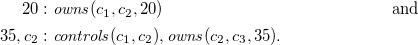 \begin{align*}20 &: {\mathit{owns}}(c_1,c_2,20) & \text{and}\\35,c_2 &: {\mathit{controls}}(c_1,c_2), {\mathit{owns}}(c_2,c_3,35).\end{align*}
We now turn to the semantics of aggregates as introduced by Ferraris (Reference Ferraris2011) but follow its adaptation to closed aggregates by Gebser et al. (Reference Gebser, Harrison, Kaminski, Lifschitz and Schaub2015a): Let a be a closed aggregate of form (8) and E be its set of aggregate elements. We say that a set $D \subseteq {{\mathrm{Inst}}(E)}$
of its elements’ instances justifies a, written
$D \subseteq {{\mathrm{Inst}}(E)}$
of its elements’ instances justifies a, written $D \triangleright a$
, if
$D \triangleright a$
, if $f({H(D)}) \prec s$
holds.
$f({H(D)}) \prec s$
holds.
An aggregate a is monotone whenever $D_1\triangleright a$
implies
$D_1\triangleright a$
implies $D_2\triangleright a$
for all
$D_2\triangleright a$
for all $D_1 \subseteq D_2 \subseteq {{\mathrm{Inst}}(E)}$
, and accordingly a is antimonotone if
$D_1 \subseteq D_2 \subseteq {{\mathrm{Inst}}(E)}$
, and accordingly a is antimonotone if $D_2\triangleright a$
implies
$D_2\triangleright a$
implies $D_1\triangleright a$
for all
$D_1\triangleright a$
for all $D_1 \subseteq D_2 \subseteq {{\mathrm{Inst}}(E)}$
.
$D_1 \subseteq D_2 \subseteq {{\mathrm{Inst}}(E)}$
.
We observe the following monotonicity properties.
Proposition 22 (Harrison et al. Reference Harrison, Lifschitz and Yang2014)
-
Aggregates over functions
${\mathrm{\#sum}^+}$
and #count together with relations
$>$
and
$\geq$
are monotone. -
Aggregates over functions
${\mathrm{\#sum}^+}$
and #count together with relations
$<$
and
$\leq$
are antimonotone. -
Aggregates over function
${\mathrm{\#sum}^-}$
have the same monotonicity properties as
${\mathrm{\#sum}^+}$
aggregates with the complementary relation.


Next, we give the translation ${\tau}$
from aggregate programs to
${\tau}$
from aggregate programs to ${\mathcal{R}}$
-programs, derived from the ones of Ferraris (Reference Ferraris2011) and Harrison et al. (Reference Harrison, Lifschitz and Yang2014):
${\mathcal{R}}$
-programs, derived from the ones of Ferraris (Reference Ferraris2011) and Harrison et al. (Reference Harrison, Lifschitz and Yang2014):
For a closed literal l, we have
 \begin{align*}{{\tau}(l)} & = l\text{,}\end{align*}
for a closed comparison l of form (6), we have
 \begin{align*}{{\tau}(l)} & = \begin{cases}\top & \text{if $\prec$ holds between $t_1$ and $t_2$}\\\bot & \text{otherwise}\end{cases}\end{align*}
and for a set L of closed literals, comparisons and aggregates, we have
 \begin{align*}{{\tau}(L)} &= {\{ {{\tau}(l)} \mid l \in L \}}\text{.}\end{align*}
For a closed aggregate a of form (8) and its set E of aggregate elements, we have
 \begin{align}{{\tau}(a)} & = {\{{{\tau}(D)}^\wedge \rightarrow {{\tau}_{a}(D)}^\vee \mid D \subseteq {{\mathrm{Inst}}(E)}, D \mathrel{\not\triangleright} a \}}^\wedge,\end{align}
where
 \begin{align*}{{\tau}_{a}(D)} & = {{\tau}({{\mathrm{Inst}}(E)} \setminus D)}\text{ for $D \subseteq {{\mathrm{Inst}}(E)}$,}\\[2pt]{{\tau}(D)} & = {\{{{\tau}(e)} \mid e \in D\}}\text{ for $D \subseteq {{\mathrm{Inst}}(E)}$, and}\\[2pt]{{\tau}(e)} & = {{{\tau}({B(e)})}}^\wedge \text{ for $e \in {{\mathrm{Inst}}(E)}$}.\end{align*}
For a closed aggregate rule r, we have
 \begin{align*}{{\tau}(r)} & = {{\tau}({H(r)})} \leftarrow {{\tau}({B(r)})}^\wedge.\end{align*}
For an aggregate program P, we have
 \begin{align}{{\tau}(P)} & = \{{{\tau}(r)} \mid r \in {{\mathrm{Inst}}(P)} \}.\end{align}
While aggregate programs like P are finite sets of (non-ground) rules, ${{\tau}(P)}$
can be infinite and contain (ground) infinitary expressions. Observe that
${{\tau}(P)}$
can be infinite and contain (ground) infinitary expressions. Observe that ${{\tau}(P)}$
is an
${{\tau}(P)}$
is an ${\mathcal{R}}$
-program. In fact, only the translation of aggregates introduces
${\mathcal{R}}$
-program. In fact, only the translation of aggregates introduces ${\mathcal{R}}$
-formulas; rules without aggregates form
${\mathcal{R}}$
-formulas; rules without aggregates form ${\mathcal{N}}$
-programs.
${\mathcal{N}}$
-programs.
Example 11 To illustrate Ferraris’ approach to the semantics of aggregates, consider a count aggregate a of form
 \begin{align*}{\mathrm{\#count} \{ {X : p(X)} \} \geq n}.\end{align*}
Since the aggregate is non-ground, the set G of its element’s instances consists of all ${t : p(t)}$
for each ground term t.
${t : p(t)}$
for each ground term t.
The count aggregate cannot be justified by any subset D of G satisfying $|\{t \mid {t : p(t)} \in D\}| < n$
, or
$|\{t \mid {t : p(t)} \in D\}| < n$
, or $D \mathrel{\not\triangleright} a$
for short. Accordingly, we have that
$D \mathrel{\not\triangleright} a$
for short. Accordingly, we have that ${{\tau}(a)}$
is the conjunction of all formulas
${{\tau}(a)}$
is the conjunction of all formulas
 \begin{align}{\{ p(t) \mid {t : p(t)} \in D \}}^\wedge& \rightarrow {\{ p(t) \mid {t : p(t)} \in (G \setminus D) \}}^\vee\end{align}
such that $D \subseteq G$
and
$D \subseteq G$
and $D \mathrel{\not\triangleright} a$
. Restricting the set of ground terms to the numerals 1,2,3 and letting
$D \mathrel{\not\triangleright} a$
. Restricting the set of ground terms to the numerals 1,2,3 and letting $n=2$
results in the formulas
$n=2$
results in the formulas
 \begin{align*}\top & \rightarrow p(1) \vee p(2) \vee p(3),\\p(1) & \rightarrow p(2) \vee p(3),\\\end{align*}
 \begin{align*}p(2) & \rightarrow p(1) \vee p(3), \text{ and }\\p(3) & \rightarrow p(1) \vee p(2).\end{align*}
Note that a smaller number of ground terms than n yields an unsatisfiable set of formulas.
However, it turns out that a Ferraris-style translation of aggregates (Ferraris Reference Ferraris2011; Harrison et al. Reference Harrison, Lifschitz and Yang2014) is too weak for propagating monotone aggregates in our id-based setting. That is, when propagating possible atoms (i.e., the second component of the well-founded model), an id-reduct may become satisfiable although the original formula is not. So, we might end up with too many possible atoms and a well-founded model that is not as precise as it could be. To see this, consider the following example.
Example 12 For some $m,n \geq 0$
, the program
$m,n \geq 0$
, the program ${{P}_{m,n}}$
consists of the following rules:
${{P}_{m,n}}$
consists of the following rules:
 \begin{align*}p(i) & \leftarrow {\neg} q(i) & & \text{ for } 1 \leq i \leq m\\[3pt]q(i) & \leftarrow {\neg} p(i) & & \text{ for } 1 \leq i \leq m\\[3pt]r & \leftarrow {\mathrm{\#count} \{ {X : p(X)} \} \geq n}.\end{align*}
Given the ground instances G of the aggregate’s elements and some two-valued interpretation I, observe that
 \begin{align*}& {{{\tau}({\mathrm{\#count} \{ {X : p(X)} \} \geq n})}_{I}}\end{align*}
is classically equivalent to
 \begin{align}& {{{\tau}({\mathrm{\#count} \{ {X : p(X)} \} \geq n})}_{I}} \vee {\{ p(t) \in {B(G)} \mid p(t) \notin I \}}^\vee.\end{align}
To see this, observe that the formula obtained via ${\tau}$
for the aggregate in the last rule’s body consists of positive occurrences of implications of the form
${\tau}$
for the aggregate in the last rule’s body consists of positive occurrences of implications of the form $\mathcal{G}^\wedge \rightarrow \mathcal{H}^\vee$
where either
$\mathcal{G}^\wedge \rightarrow \mathcal{H}^\vee$
where either $p(t) \in \mathcal{G}$
or
$p(t) \in \mathcal{G}$
or $p(t) \in \mathcal{H}$
. The id-reduct makes all such implications with some
$p(t) \in \mathcal{H}$
. The id-reduct makes all such implications with some $p(t) \in \mathcal{G}$
such that
$p(t) \in \mathcal{G}$
such that $p(t) \notin I$
true because their antecedent is false. All of the remaining implications in the id-reduct are equivalent to
$p(t) \notin I$
true because their antecedent is false. All of the remaining implications in the id-reduct are equivalent to $\mathcal{H}^\vee$
where
$\mathcal{H}^\vee$
where $\mathcal{H}$
contains all
$\mathcal{H}$
contains all $p(t) \notin I$
. Thus, we can factor out the formula on the right-hand side of (12).
$p(t) \notin I$
. Thus, we can factor out the formula on the right-hand side of (12).
Next, observe that for $1 \leq m < n$
, the four-valued interpretation
$1 \leq m < n$
, the four-valued interpretation $(I,J) = (\emptyset, {H({{\tau}({{P}_{m,n}})})})$
is the well-founded model of
$(I,J) = (\emptyset, {H({{\tau}({{P}_{m,n}})})})$
is the well-founded model of ${{P}_{m,n}}$
:
${{P}_{m,n}}$
:
 \begin{align*}{{{S}_{{{\tau}({{P}_{m,n}})}}}(J)} & = I\text{ and}\\[3pt]{{{S}_{{{\tau}({{P}_{m,n}})}}}(I)} & = J.\end{align*}
Ideally, atom r should not be among the possible atoms because it can never be in a stable model. Nonetheless, it is due to the second disjunct in (12).
Note that not just monotone aggregates exhibit this problem. In general, we get for a closed aggregate a with elements E and an interpretation I that
 \begin{align*}{{{\tau}(a)}_{I}} \text{ is classically equivalent to } {{{\tau}(a)}_{I}} \vee {\{c \in {B({{\mathrm{Inst}}(E)})} \mid I \not\models c\}}^\vee.\end{align*}
The second disjunct is undesirable when propagating possible atoms.
To address this shortcoming, we augment the aggregate translation so that it provides stronger propagation. The result of the augmented translation is strongly equivalent to that of the original translation (cf. Proposition 23). Thus, even though we get more precise well-founded models, the stable models are still contained in them.
Definition 9 We define ${\pi}$
as the translation obtained from
${\pi}$
as the translation obtained from ${\tau}$
by replacing the case of closed aggregates in (9) by the following:
${\tau}$
by replacing the case of closed aggregates in (9) by the following:
For a closed aggregate a of form (8) and its set E of aggregate elements, we have
 \begin{align*}{{\pi}(a)} & = {\{ {{{\tau}(D)}}^\wedge \rightarrow {{{\pi}_{a}}(D)}^\vee \mid D \subseteq {{\mathrm{Inst}}(E)}, D \mathrel{\not\triangleright} a \}}^\wedge,\\\end{align*}
where
 \begin{align*}{{{\pi}_{a}}(D)} & = \{ {{{\tau}(C)}}^\wedge \mid C \subseteq {{\mathrm{Inst}}(E)} \setminus D, C \cup D \triangleright a \}\text{ for } D \subseteq {{\mathrm{Inst}}(E)}.\end{align*}
Note that just as ${\tau}$
also
${\tau}$
also ${\pi}$
is recursively applied to the whole program.
${\pi}$
is recursively applied to the whole program.
Let us illustrate the modified translation by revisiting Example 11.
Example 13 Let us reconsider the count aggregate a:
 \begin{align*}{\mathrm{\#count} \{ {X : p(X)} \} \geq n}.\end{align*}
As with ${{\tau}(a)}$
in Example 11,
${{\tau}(a)}$
in Example 11, ${{\pi}(a)}$
yields a conjunction of formulas, one conjunct for each set
${{\pi}(a)}$
yields a conjunction of formulas, one conjunct for each set $D\subseteq {{\mathrm{Inst}}(E)}$
satisfying
$D\subseteq {{\mathrm{Inst}}(E)}$
satisfying $D\mathrel{\not\triangleright} a$
of the form:
$D\mathrel{\not\triangleright} a$
of the form:
 \begin{align}{\{ {B(e)} \mid e \in D\}}^\wedge\rightarrow{\big\{ {\{ {B(e)} \mid e \in (C \setminus D) \}}^\wedge \mid C \triangleright a, D \subseteq C \subseteq {{\mathrm{Inst}}(E)} \big\}}^\vee.\end{align}
Restricting again the set of ground terms to the numerals 1,2,3 and letting $n=2$
results now in the formulas
$n=2$
results now in the formulas
 \begin{align*}\top & \rightarrow (p(1) \wedge p(2)) \vee (p(1) \wedge p(3)) \vee (p(2)\wedge p(3))\vee(p(1)\wedge p(2)\wedge p(3)),\\p(1) & \rightarrow p(2) \vee p(3) \vee (p(2) \wedge p(3)),\\p(2) & \rightarrow p(1) \vee p(3) \vee (p(1) \wedge p(3)), \text{ and }\\p(3) & \rightarrow p(1) \vee p(2) \vee (p(1) \wedge p(2)).\end{align*}
Note that the last disjunct can be dropped from each rule’s consequent. And as above, a smaller number of ground terms than n yields an unsatisfiable set of formulas.
The next result ensures that ${{\tau}(P)}$
and
${{\tau}(P)}$
and ${{\pi}(P)}$
have the same stable models for any aggregate program P.
${{\pi}(P)}$
have the same stable models for any aggregate program P.
Proposition 23 Let a be a closed aggregate.
Then, ${{\tau}(a)}$
and
${{\tau}(a)}$
and ${{\pi}(a)}$
are strongly equivalent.
${{\pi}(a)}$
are strongly equivalent.
The next example illustrates that we get more precise well-founded models using the strongly equivalent refined translation.
Example 14 Reconsider Program ${{P}_{m,n}}$
from Example 12.
${{P}_{m,n}}$
from Example 12.
As above, we apply the well-founded operator to program ${{P}_{m,n}}$
for
${{P}_{m,n}}$
for $m < n$
and four-valued interpretation
$m < n$
and four-valued interpretation $(I,J) = (\emptyset, {H({{\pi}({{P}_{m,n}})})})$
:
$(I,J) = (\emptyset, {H({{\pi}({{P}_{m,n}})})})$
:
 \begin{align*}{{{S}_{{{\pi}({{P}_{m,n}})}}}(J)} & = I \text{ and }\\{{{S}_{{{\pi}({{P}_{m,n}})}}}(I)} & = J \setminus \{ r \}.\end{align*}
Unlike before, r is now found to be false since it does not belong to ${{{S}_{{{\pi}({{P}_{m,n}})}}}(\emptyset)}$
.
${{{S}_{{{\pi}({{P}_{m,n}})}}}(\emptyset)}$
.
To see this, we can take advantage of the following proposition.
Proposition 24 Let a be a closed aggregate.
If a is monotone, then ${{{\pi}(a)}_{I}}$
is classically equivalent to
${{{\pi}(a)}_{I}}$
is classically equivalent to ${{\pi}(a)}$
for any two-valued interpretation I.
${{\pi}(a)}$
for any two-valued interpretation I.
Note that ${{\pi}(a)}$
is a negative formula whenever a is antimonotone; cf. Proposition 36.
${{\pi}(a)}$
is a negative formula whenever a is antimonotone; cf. Proposition 36.
Let us briefly return to Example 14. We now observe that ${{{\pi}(a)}_{I}}={{\pi}(a)}$
for
${{{\pi}(a)}_{I}}={{\pi}(a)}$
for $a={\mathrm{\#count} \{ {X : p(X)} \} \geq} n$
and any interpretation I in view of the last proposition. Hence, our refined translation
$a={\mathrm{\#count} \{ {X : p(X)} \} \geq} n$
and any interpretation I in view of the last proposition. Hence, our refined translation ${\pi}$
avoids the problematic disjunct in Equation (12) on the right. By Proposition 23, we can use
${\pi}$
avoids the problematic disjunct in Equation (12) on the right. By Proposition 23, we can use ${{\pi}({{P}_{m,n}})}$
instead of
${{\pi}({{P}_{m,n}})}$
instead of ${{\tau}({{P}_{m,n}})}$
; both formulas have the same stable models.
${{\tau}({{P}_{m,n}})}$
; both formulas have the same stable models.
Using Proposition 24, we augment the translation ${\pi}$
to replace monotone aggregates a by the strictly positive formula
${\pi}$
to replace monotone aggregates a by the strictly positive formula ${{{\pi}(a)}_{\emptyset}}$
. That is, we only keep the implication with the trivially true antecedent in the aggregate translation (cf. Section 5).
${{{\pi}(a)}_{\emptyset}}$
. That is, we only keep the implication with the trivially true antecedent in the aggregate translation (cf. Section 5).
While ${\pi}$
improves on propagation, it may still produce infinitary
${\pi}$
improves on propagation, it may still produce infinitary ${\mathcal{R}}$
-formulas when applied to aggregates. This issue is addressed by restricting the translation to a set of (possible) atoms.
${\mathcal{R}}$
-formulas when applied to aggregates. This issue is addressed by restricting the translation to a set of (possible) atoms.
Definition 10 Let J be a two-valued interpretation. We define the translation ${{\pi}_{J}}$
as the one obtained from
${{\pi}_{J}}$
as the one obtained from ${\tau}$
by replacing the case of closed aggregates in (9) by the following:
${\tau}$
by replacing the case of closed aggregates in (9) by the following:
For a closed aggregate a of form (8) and its set E of aggregate elements, we have
 \begin{align*}{{{\pi}_{J}}(a)} & = {\{ {{\tau}(D)}^\wedge \rightarrow {{{\pi}_{a,J}}(D)}^\vee \mid D \subseteq {{{\mathrm{Inst}}(E)}|_{J}}, D \mathrel{\not\triangleright} a \}}^\wedge,\end{align*}
where
 \begin{align*}{{{\pi}_{a,J}}(D)} & = {\{ {{\tau}(C)}^\wedge \mid C \subseteq {{{\mathrm{Inst}}(E)}|_{J}} \setminus D, C \cup D \triangleright a \}}\text{ and }\\{{{\mathrm{Inst}}(E)}|_{J}} & = \{ e \in {{\mathrm{Inst}}(E)} \mid {B(e)} \subseteq J \}.\end{align*}
Note that ${{{\pi}_{J}}(a)}$
is a finitary formula whenever J is finite.
${{{\pi}_{J}}(a)}$
is a finitary formula whenever J is finite.
Clearly, ${{\pi}_{J}}$
also conforms to
${{\pi}_{J}}$
also conforms to ${\pi}$
except for the restricted translation for aggregates defined above. The next proposition elaborates this by showing that
${\pi}$
except for the restricted translation for aggregates defined above. The next proposition elaborates this by showing that ${{\pi}_{J}}$
and
${{\pi}_{J}}$
and ${\pi}$
behave alike whenever J limits the set of possible atoms.
${\pi}$
behave alike whenever J limits the set of possible atoms.
Theorem 25 Let a be a closed aggregate, and $I \subseteq J$
and
$I \subseteq J$
and $X \subseteq J$
be two-valued interpretations. Then,
$X \subseteq J$
be two-valued interpretations. Then,
-
(a)
$X \models {{\pi}(a)}$
iff
$X \models {{{\pi}_{J}}(a)}$
, -
(b)
$X \models {{{\pi}(a)}_{I}}$
iff
$X \models {{{{\pi}_{J}}(a)}_{I}}$
, and -
(c)
$X \models {{{\pi}(a)}^{I}}$
iff
$X \models {{{{\pi}_{J}}(a)}^{I}}$
.


In view of Proposition 23, this result extends to Ferraris’ original aggregate translation (Ferraris Reference Ferraris2011; Harrison et al. Reference Harrison, Lifschitz and Yang2014).
The next example illustrates how a finitary formula can be obtained for an aggregate, despite a possibly infinite set of terms in the signature.
Example 15 Let ${{P}_{m,n}}$
be the program from Example 12. The well-founded model (I,J) of
${{P}_{m,n}}$
be the program from Example 12. The well-founded model (I,J) of ${{\pi}({{P}_{m,n}})}$
is
${{\pi}({{P}_{m,n}})}$
is $(\emptyset, {H({{\pi}({{P}_{m,n}})})})$
if
$(\emptyset, {H({{\pi}({{P}_{m,n}})})})$
if $n \leq m$
.
$n \leq m$
.
The translation ${{{\pi}_{J}}({{P}_{3,2}})}$
consists of the rules
${{{\pi}_{J}}({{P}_{3,2}})}$
consists of the rules
 \begin{align*}p(1) & \leftarrow {\neg} q(1), &q(1) & \leftarrow {\neg} p(1), \\[3pt]p(2) & \leftarrow {\neg} q(2), &q(2) & \leftarrow {\neg} p(2), \\[3pt]p(3) & \leftarrow {\neg} q(3), &q(3) & \leftarrow {\neg} p(3), \text{ and }\\[3pt]r & \leftarrow \pi_{J}({\mathrm{\#count} \{ {X : p(X)} \} \geq 2}),\end{align*}
where the aggregate translation corresponds to the conjunction of the formulas in Example 13. Note that the translation ${{\pi}({{P}_{3,2}})}$
depends on the signature whereas the translation
${{\pi}({{P}_{3,2}})}$
depends on the signature whereas the translation ${{{\pi}_{J}}({{P}_{3,2}})}$
is fixed by the atoms in J.
${{{\pi}_{J}}({{P}_{3,2}})}$
is fixed by the atoms in J.
Importantly, Proposition 25 shows that given a finite (approximation of the) well-founded model of an ${\mathcal{R}}$
-program, we can replace aggregates with finitary formulas. Moreover, in this case, Theorem 9 and Proposition 23 together indicate how to turn a program with aggregates into a semantically equivalent finite
${\mathcal{R}}$
-program, we can replace aggregates with finitary formulas. Moreover, in this case, Theorem 9 and Proposition 23 together indicate how to turn a program with aggregates into a semantically equivalent finite ${\mathcal{R}}$
-program with finitary formulas as bodies. That is, given a finite well-founded model of an
${\mathcal{R}}$
-program with finitary formulas as bodies. That is, given a finite well-founded model of an ${\mathcal{R}}$
-program, the program simplification from Definition 1 results in a finite program and the aggregate translation from Definition 10 produces finitary formulas only.
${\mathcal{R}}$
-program, the program simplification from Definition 1 results in a finite program and the aggregate translation from Definition 10 produces finitary formulas only.
This puts us in a position to outline how and when (safe non-ground) aggregate programs can be turned into equivalent finite ground programs consisting of finitary subformulas only. To this end, consider an aggregate program P along with the well-founded model (I,J) of ${{\pi}(P)}$
. We have already seen in Corollary 10 that
${{\pi}(P)}$
. We have already seen in Corollary 10 that ${{\pi}(P)}$
and its simplification
${{\pi}(P)}$
and its simplification ${{{\pi}(P)}^{I,J}}$
have the same stable models, just like
${{{\pi}(P)}^{I,J}}$
have the same stable models, just like ${{{\pi}(P)}^{I,J}}$
and its counterpart
${{{\pi}(P)}^{I,J}}$
and its counterpart ${{{{\pi}_{J}}(P)}^{I,J}}$
in view of Proposition 25.
${{{{\pi}_{J}}(P)}^{I,J}}$
in view of Proposition 25.
Now, if (I,J) is finite, then ${{{\pi}(P)}^{I,J}}$
is finite, too. Seen from the perspective of grounding, the safety of all rules in P implies that all global variables appear in positive body literals. Thus, the number of ground instances of each rule in
${{{\pi}(P)}^{I,J}}$
is finite, too. Seen from the perspective of grounding, the safety of all rules in P implies that all global variables appear in positive body literals. Thus, the number of ground instances of each rule in ${{{\pi}(P)}^{I,J}}$
is determined by the number of possible substitutions for its global variables. Clearly, there are only finitely many possible substitutions such that all positive body literals are satisfied by a finite interpretation J (cf. Definition 1). Furthermore, if J is finite, aggregate translations in
${{{\pi}(P)}^{I,J}}$
is determined by the number of possible substitutions for its global variables. Clearly, there are only finitely many possible substitutions such that all positive body literals are satisfied by a finite interpretation J (cf. Definition 1). Furthermore, if J is finite, aggregate translations in ${{{{\pi}_{J}}(P)}^{I,J}}$
introduce finitary subformulas only. Thus, in this case, we obtain from P a finite set of rules with finitary propositional formulas as bodies, viz.
${{{{\pi}_{J}}(P)}^{I,J}}$
introduce finitary subformulas only. Thus, in this case, we obtain from P a finite set of rules with finitary propositional formulas as bodies, viz. ${{{{\pi}_{J}}(P)}^{I,J}}$
, that has the same stable models as
${{{{\pi}_{J}}(P)}^{I,J}}$
, that has the same stable models as ${{\pi}(P)}$
(as well as
${{\pi}(P)}$
(as well as ${{\tau}(P)}$
, the traditional Ferraris-style semantics of P (Ferraris Reference Ferraris2011; Harrison et al. Reference Harrison, Lifschitz and Yang2014)).
${{\tau}(P)}$
, the traditional Ferraris-style semantics of P (Ferraris Reference Ferraris2011; Harrison et al. Reference Harrison, Lifschitz and Yang2014)).
An example of a class of aggregate programs inducing finite well-founded models as above consists of programs over a signature with nullary function symbols only. Any such program can be turned into an equivalent finite set of propositional rules with finitary bodies.
5 Dependency analysis
We now further refine our semantic approach to reflect actual grounding processes. In fact, modern grounders process programs on-the-fly by grounding one rule after another without storing any rules. At the same time, they try to determine certain, possible, and false atoms. Unfortunately, well-founded models cannot be computed on-the-fly, which is why we introduce below the concept of an approximate model. More precisely, we start by defining instantiation sequences of (non-ground) aggregate programs based on their rule dependencies. We show that approximate models of instantiation sequences are underapproximations of the well-founded model of the corresponding sequence of (ground) ${\mathcal{R}}$
-programs, as defined in Section 3. The precision of both types of models coincides on stratified programs. We illustrate our concepts comprehensively at the end of this section in Example 19 and 20.
${\mathcal{R}}$
-programs, as defined in Section 3. The precision of both types of models coincides on stratified programs. We illustrate our concepts comprehensively at the end of this section in Example 19 and 20.
To begin with, we extend the notion of positive and negative literals to aggregate programs. For atoms a, we define $a^+ = {({\neg} a)}^- = \{a\}$
and
$a^+ = {({\neg} a)}^- = \{a\}$
and $a^- = {({\neg} a)}^+ = \emptyset$
. For comparisons a, we define
$a^- = {({\neg} a)}^+ = \emptyset$
. For comparisons a, we define $a^+ = a^- = \emptyset$
. For aggregates a with elements E, we define positive and negative atom occurrences, using Proposition 24 to refine the case for monotone aggregates:
$a^+ = a^- = \emptyset$
. For aggregates a with elements E, we define positive and negative atom occurrences, using Proposition 24 to refine the case for monotone aggregates:
-
$a^+ = \bigcup_{e \in E} {B(e)}$
,
-
$a^- = \emptyset$
if a is monotone, and
-
$a^- = \bigcup_{e \in E} {B(e)}$
if a is not monotone.


For a set of body literals B, we define $B^+ = \bigcup_{b \in B}b^+$
and
$B^+ = \bigcup_{b \in B}b^+$
and $B^- = \bigcup_{b \in B}b^-$
, as well as
$B^- = \bigcup_{b \in B}b^-$
, as well as $B^\pm=B^+\cup B^-$
.
$B^\pm=B^+\cup B^-$
.
We see in the following, that a special treatment of monotone aggregates yields better approximations of well-founded models. A similar case could be made for antimonotone aggregates but had led to a more involved algorithmic treatment.
Inter-rule dependencies are determined via the predicates appearing in their heads and bodies. We define ${\mathrm{pred}(a)}$
to be the predicate symbol associated with atom a and
${\mathrm{pred}(a)}$
to be the predicate symbol associated with atom a and ${\mathrm{pred}(A)} = \{ {\mathrm{pred}(a)} \mid a \in A \}$
for a set A of atoms. An aggregate rule
${\mathrm{pred}(A)} = \{ {\mathrm{pred}(a)} \mid a \in A \}$
for a set A of atoms. An aggregate rule $r_1$
depends on another aggregate rule
$r_1$
depends on another aggregate rule $r_2$
if
$r_2$
if ${\mathrm{pred}({H(r_2)})} \in {\mathrm{pred}({{B(r_1)}}^\pm)}$
. Rule
${\mathrm{pred}({H(r_2)})} \in {\mathrm{pred}({{B(r_1)}}^\pm)}$
. Rule $r_1$
depends positively or negatively on
$r_1$
depends positively or negatively on $r_2$
if
$r_2$
if ${\mathrm{pred}({H(r_2)})} \in {\mathrm{pred}({B(r_1)}^+)}$
or
${\mathrm{pred}({H(r_2)})} \in {\mathrm{pred}({B(r_1)}^+)}$
or ${\mathrm{pred}({H(r_2)})} \in {\mathrm{pred}({{B(r_2)}}^-)}$
, respectively.
${\mathrm{pred}({H(r_2)})} \in {\mathrm{pred}({{B(r_2)}}^-)}$
, respectively.
For simplicity, we first focus on programs without aggregates in examples and delay a full example with aggregates until the end of the section.
Example 16 Let us consider the following rules from the introductory example:
 \begin{align}u(1) &\end{align}
 \begin{align}p(X) & \leftarrow {\neg} q(X) \wedge u(X)\end{align}
 \begin{align}q(X) & \leftarrow {\neg} p(X) \wedge v(X).\end{align}
We first determine the rule heads and positive and negative atom occurrences in rule bodies:
 \begin{align*}{H(r_1)} & = u(1) &{B(r_1)}^+ & = \emptyset &{B(r_1)}^- & = \emptyset \\{H(r_2)} & = p(X) &{B(r_2)}^+ & = \{ u(X) \} &{B(r_2)}^- & = \{ q(X) \} \\{H(r_3)} & = q(X) &{B(r_3)}^+ & = \{ v(X) \} &{B(r_3)}^- & = \{ p(X) \}.\end{align*}
With this, we infer the corresponding predicates:
 \begin{align*}{\mathrm{pred}({H(r_1)})} & = u/1 &{\mathrm{pred}({B(r_1)}^+)} & = \emptyset &{\mathrm{pred}({B(r_1)}^-)} & = \emptyset \\[2pt]{\mathrm{pred}({H(r_2)})} & = p/1 &{\mathrm{pred}({B(r_2)}^+)} & = \{ u/1 \} &{\mathrm{pred}({B(r_2)}^-)} & = \{ q/1 \} \\[2pt]{\mathrm{pred}({H(r_3)})} & = q/1 &{\mathrm{pred}({B(r_3)}^+)} & = \{ v/1 \} &{\mathrm{pred}({B(r_3)}^-)} & = \{ p/1 \}.\end{align*}
We see that $r_2$
depends positively on
$r_2$
depends positively on $r_1$
and that
$r_1$
and that $r_2$
and
$r_2$
and $r_3$
depend negatively on each other. View Figure 1 in Example 17 for a graphical representation of these inter-rule dependencies.
$r_3$
depend negatively on each other. View Figure 1 in Example 17 for a graphical representation of these inter-rule dependencies.
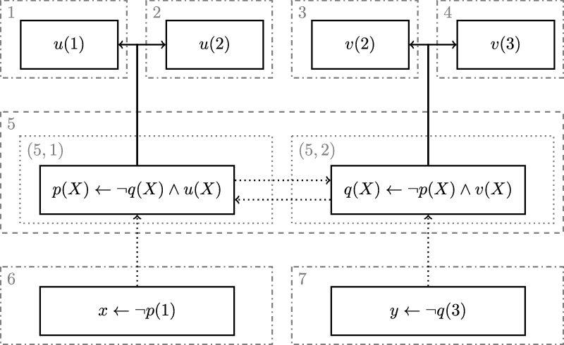
Fig. 1. Rule dependencies for Example 19.
The strongly connected components of an aggregate program P are the equivalence classes under the transitive closure of the dependency relation between all rules in P. A strongly connected component ${{P}_{1}}$
depends on another strongly connected component
${{P}_{1}}$
depends on another strongly connected component ${{P}_{2}}$
if there is a rule in
${{P}_{2}}$
if there is a rule in ${{P}_{1}}$
that depends on some rule in
${{P}_{1}}$
that depends on some rule in ${{P}_{2}}$
. The transitive closure of this relation is antisymmetric.
${{P}_{2}}$
. The transitive closure of this relation is antisymmetric.
A strongly connected component of an aggregate program is unstratified if it depends negatively on itself or if it depends on an unstratified component. A component is stratified if it is not unstratified.
A topological ordering of the strongly connected components is then used to guide grounding.
For example, the sets $\{r_1\}$
and
$\{r_1\}$
and $\{r_2, r_3\}$
of rules from Example 16 are strongly connected components in a topological order. There is only one topological order because
$\{r_2, r_3\}$
of rules from Example 16 are strongly connected components in a topological order. There is only one topological order because $r_2$
depends on
$r_2$
depends on $r_1$
. While the first component is stratified, the second component is unstratified because
$r_1$
. While the first component is stratified, the second component is unstratified because $r_2$
and
$r_2$
and $r_3$
depend negatively on each other.
$r_3$
depend negatively on each other.
Definition 11 We define an instantiation sequence for P as a sequence ${{{({{P}_{i}})}_{i \in \mathbb{I}}}}$
of its strongly connected components such that
${{{({{P}_{i}})}_{i \in \mathbb{I}}}}$
of its strongly connected components such that $i < j$
if
$i < j$
if ${{P}_{j}}$
depends on
${{P}_{j}}$
depends on ${{P}_{i}}$
.
${{P}_{i}}$
.
Note that the components can always be well ordered because aggregate programs consist of finitely many rules.
The consecutive construction of the well-founded model along an instantiation sequence results in the well-founded model of the entire program.
Theorem 26 Let ${{{({{P}_{i}})}_{i \in \mathbb{I}}}}$
be an instantiation sequence for aggregate program P.
${{{({{P}_{i}})}_{i \in \mathbb{I}}}}$
be an instantiation sequence for aggregate program P.
Then, ${\mathit{WM}({{({{\pi}(P_i)})}_{i\in\mathbb{I}}})} = {\mathit{WM}({{\pi}(P)})}$
.
${\mathit{WM}({{({{\pi}(P_i)})}_{i\in\mathbb{I}}})} = {\mathit{WM}({{\pi}(P)})}$
.
Example 17 The following example shows how to split an aggregate program into an instantiation sequence and gives its well-founded model. Let P be the following aggregate program, extending the one from the introductory section:
 \begin{align*}u(1) & &u(2) & \\v(2) & &v(3) & \\p(X) & \leftarrow {\neg} q(X) \wedge u(X) &q(X) & \leftarrow {\neg} p(X) \wedge v(X) \\x & \leftarrow {\neg} p(1) &y & \leftarrow {\neg} q(3).\end{align*}
We have already seen how to determine inter-rule dependencies in Example 16. A possible instantiation sequence for program P is given in Figure 1. Rules are depicted in solid boxes. Solid and dotted edges between such boxes depict positive and negative dependencies between the corresponding rules, respectively. Dashed and dashed/dotted boxes represent components in the instantiation sequence (we ignore dotted boxes for now but turn to them in Example 18). The number in the corner of a component box indicates the index in the corresponding instantiation sequence.
For $F = \{u(1),u(2),v(2),v(3)\}$
, the well-founded model of
$F = \{u(1),u(2),v(2),v(3)\}$
, the well-founded model of ${{\pi}(P)}$
is
${{\pi}(P)}$
is
 \begin{align*}{\mathit{WM}({{\pi}(P)})} &= (\{p(1),q(3)\},\{p(1),p(2),q(2),q(3)\}) \sqcup F.\end{align*}
By Theorem 26, the ground sequence ${{{({{\tau}({{P}_{i}})})}_{i \in \mathbb{I}}}}$
has the same well-founded model as
${{{({{\tau}({{P}_{i}})})}_{i \in \mathbb{I}}}}$
has the same well-founded model as ${{\pi}(P)}$
:
${{\pi}(P)}$
:
 \begin{align*}{\mathit{WM}({{({{\pi}(P)})}_{i\in\mathbb{I}}})} &= (\{p(1),q(3)\},\{p(1),p(2),q(2),q(3)\}) \sqcup F.\end{align*}
Note that the set F comprises the facts derived from stratified components. In fact, for stratified components, the set of external atoms (3) is empty. We can use Corollary 20 to confirm that the well founded model (F,F) of sequence ${{({{\pi}({{P}_{i}})})}_{1 \leq i \leq 4}}$
is total. In fact, each of the intermediate interpretations (5) is total and can be computed with just one application of the stable operator. For example,
${{({{\pi}({{P}_{i}})})}_{1 \leq i \leq 4}}$
is total. In fact, each of the intermediate interpretations (5) is total and can be computed with just one application of the stable operator. For example, ${I_{1}}={J_{1}}=\{u(1)\}$
for component
${I_{1}}={J_{1}}=\{u(1)\}$
for component ${{P}_{1}}$
.
${{P}_{1}}$
.
We further refine instantiation sequences by partitioning each component along its positive dependencies.
Definition 12 Let P be an aggregate program and ${{{({{P}_{i}})}_{i \in \mathbb{I}}}}$
be an instantiation sequence for P. Furthermore, for each
${{{({{P}_{i}})}_{i \in \mathbb{I}}}}$
be an instantiation sequence for P. Furthermore, for each $i \in \mathbb{I}$
, let
$i \in \mathbb{I}$
, let ${{({{P}_{i,j}})}_{j \in \mathbb{I}_i}}$
be an instantiation sequence of
${{({{P}_{i,j}})}_{j \in \mathbb{I}_i}}$
be an instantiation sequence of ${{P}_{i}}$
considering positive dependencies only.
${{P}_{i}}$
considering positive dependencies only.
A refined instantiation sequence for P is a sequence ${{{({{P}_{i,j}})}_{(i,j) \in \mathbb{J}}}}$
where the index set
${{{({{P}_{i,j}})}_{(i,j) \in \mathbb{J}}}}$
where the index set $\mathbb{J} = \{ (i,j) \mid i \in \mathbb{I}, j \in \mathbb{I}_i \}$
is ordered lexicographically.
$\mathbb{J} = \{ (i,j) \mid i \in \mathbb{I}, j \in \mathbb{I}_i \}$
is ordered lexicographically.
We call ${{{({{P}_{i,j}})}_{(i,j) \in \mathbb{J}}}}$
a refinement of
${{{({{P}_{i,j}})}_{(i,j) \in \mathbb{J}}}}$
a refinement of ${{{({{P}_{i}})}_{i \in \mathbb{I}}}}$
.
${{{({{P}_{i}})}_{i \in \mathbb{I}}}}$
.
We define a component ${{P}_{i,j}}$
to be stratified or unstratified if the encompassing component
${{P}_{i,j}}$
to be stratified or unstratified if the encompassing component ${{P}_{i}}$
is stratified or unstratified, respectively.
${{P}_{i}}$
is stratified or unstratified, respectively.
Examples of refined instantiation sequences are given in Figures 1 and 2.
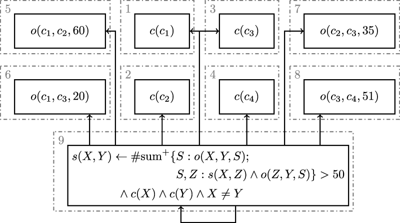
Fig. 2. Rule dependencies for the company controls encoding and instance in Example 10 where $c={\mathit{company}}$
,
$c={\mathit{company}}$
, $o={\mathit{owns}}$
, and
$o={\mathit{owns}}$
, and $s={\mathit{controls}}$
.
$s={\mathit{controls}}$
.
The advantage of such refinements is that they yield better or equal approximations (cf. Theorem 28 and Example 19). On the downside, we do not obtain that ${\mathit{WM}({{{({{P}_{i}})}_{i \in \mathbb{J}}}})}$
equals
${\mathit{WM}({{{({{P}_{i}})}_{i \in \mathbb{J}}}})}$
equals ${\mathit{WM}({{\pi}(P)})}$
for refined instantiation sequences in general.
${\mathit{WM}({{\pi}(P)})}$
for refined instantiation sequences in general.
Example 18 The refined instantiation sequence for program P from Example 17 is given in Figure 1. A dotted box indicates a component in a refined instantiation sequence. Components that cannot be refined further are depicted with a dashed/dotted box. The number or pair in the corner of a component box indicates the index in the corresponding refined instantiation sequence.
Unlike in Example 17, the well-founded model of the refined sequence of ground programs ${{{({{\tau}({{P}_{i,j}})})}_{(i,j) \in \mathbb{J}}}}$
is
${{{({{\tau}({{P}_{i,j}})})}_{(i,j) \in \mathbb{J}}}}$
is
 \begin{align*}{\mathit{WM}({{{({{\tau}({{P}_{i,j}})})}_{(i,j) \in \mathbb{J}}}})} &= (\{q(3)\},\{p(1),p(2),q(2),q(3),x\}) \sqcup F,\end{align*}
which is actually less precise than the well-founded model of P. This is because literals over ${\neg} q(X)$
are unconditionally assumed to be true because their instantiation is not yet available when
${\neg} q(X)$
are unconditionally assumed to be true because their instantiation is not yet available when ${{P}_{5,1}}$
is considered. Thus, we get
${{P}_{5,1}}$
is considered. Thus, we get $({I_{5,1}},{J_{5,1}}) = (\emptyset, \{ p(1), p(2) \})$
for the intermediate interpretation (5). Unlike this, the atom p(3) is false when considering component
$({I_{5,1}},{J_{5,1}}) = (\emptyset, \{ p(1), p(2) \})$
for the intermediate interpretation (5). Unlike this, the atom p(3) is false when considering component ${{P}_{5,2}}$
and q(3) becomes true. In fact, we get
${{P}_{5,2}}$
and q(3) becomes true. In fact, we get $({I_{5,2}},{J_{5,2}}) = (\{q(3)\}, \{ q(2), q(3) \})$
. Observe that
$({I_{5,2}},{J_{5,2}}) = (\{q(3)\}, \{ q(2), q(3) \})$
. Observe that $({I_{5}}, {J_{5}})$
from above is less precise than
$({I_{5}}, {J_{5}})$
from above is less precise than $({I_{5,1}}, {J_{5,1}}) \sqcup ({I_{5,2}}, {J_{5,2}})$
.
$({I_{5,1}}, {J_{5,1}}) \sqcup ({I_{5,2}}, {J_{5,2}})$
.
We continue with this example below and show in Example 19 that refined instantiation sequences can still be advantageous to get better approximations of well-founded models.
We have already seen in Section 3 that external atoms may lead to less precise semantic characterizations. This is just the same in the non-ground case, whenever a component comprises predicates that are defined in a following component of a refined instantiation sequence. This leads us to the concept of an approximate model obtained by overapproximating the extension of such externally defined predicates.
Definition 13 Let P be an aggregate program, $({\mathit{I\!{C}}},{\mathit{J\!{C}}})$
be a four-valued interpretation,
$({\mathit{I\!{C}}},{\mathit{J\!{C}}})$
be a four-valued interpretation, ${\mathcal{E}}$
be a set of predicates, and P’ be the program obtained from P by removing all rules r with
${\mathcal{E}}$
be a set of predicates, and P’ be the program obtained from P by removing all rules r with ${\mathrm{pred}({B(r)}^-)} \cap {\mathcal{E}} \neq \emptyset$
.
${\mathrm{pred}({B(r)}^-)} \cap {\mathcal{E}} \neq \emptyset$
.
We define the approximate model of P relative to $({\mathit{I\!{C}}},{\mathit{J\!{C}}})$
as
$({\mathit{I\!{C}}},{\mathit{J\!{C}}})$
as
 \begin{align*}{\mathit{AM}^{({\mathit{I\!{C}}},{\mathit{J\!{C}}})}_{{\mathcal{E}}}(P)} & = (I,J),\end{align*}
where
 \begin{align*}I &= {{{S}_{{{\pi}(P')}}^{{\mathit{I\!{C}}}}}({\mathit{J\!{C}}})}\text{ and }\\[2pt]J &= {{{S}_{{{\pi}(P)}}^{{\mathit{J\!{C}}}}}({\mathit{I\!{C}}} \cup I)}.\end{align*}
We keep dropping parentheses and simply write ${\mathit{AM}^{{\mathit{I\!{C}}},{\mathit{J\!{C}}}}_{{\mathcal{E}}}(P)}$
instead of
${\mathit{AM}^{{\mathit{I\!{C}}},{\mathit{J\!{C}}}}_{{\mathcal{E}}}(P)}$
instead of ${\mathit{AM}^{({\mathit{I\!{C}}},{\mathit{J\!{C}}})}_{{\mathcal{E}}}(P)}$
.
${\mathit{AM}^{({\mathit{I\!{C}}},{\mathit{J\!{C}}})}_{{\mathcal{E}}}(P)}$
.
The approximate model amounts to an immediate consequence operator, similar to the relative well-founded operator in Definition 4; it refrains from any iterative applications, as used for defining a well-founded model. More precisely, the relative stable operator is applied twice to obtain the approximate model. This is similar to Van Gelder’s alternating transformation (Van Gelder Reference Van Gelder1993). The certain atoms in I are determined by applying the operator to the ground program obtained after removing all rules whose negative body literals comprise externally defined predicates, while the possible atoms J are computed from the entire program by taking the already computed certain atoms in I into account. In this way, the approximate model may result in fewer unknown atoms than the relative well-founded operator when applied to the least precise interpretation (as an easy point of reference). How well we can approximate the certain atoms with the approximate operator depends on the set of external predicates ${\mathcal{E}}$
. When approximating the model of a program P in a sequence, the set
${\mathcal{E}}$
. When approximating the model of a program P in a sequence, the set ${\mathcal{E}}$
comprises all negative predicates occurring in P for which possible atoms have not yet been fully computed. This leads to fewer certain atoms obtained from the reduced program,
${\mathcal{E}}$
comprises all negative predicates occurring in P for which possible atoms have not yet been fully computed. This leads to fewer certain atoms obtained from the reduced program, $P'=\{r \in P\mid {\mathrm{pred}({B(r)}^-)} \cap {\mathcal{E}} = \emptyset\}$
, stripped of all rules from P that have negative body literals whose predicates occur in
$P'=\{r \in P\mid {\mathrm{pred}({B(r)}^-)} \cap {\mathcal{E}} = \emptyset\}$
, stripped of all rules from P that have negative body literals whose predicates occur in ${\mathcal{E}}$
.
${\mathcal{E}}$
.
The next theorem identifies an essential prerequisite for an approximate model of a non-ground program to be an underapproximation of the well-founded model of the corresponding ground program.
Theorem 27 Let P be an aggregate program, ${\mathcal{E}}$
be a set of predicates, and
${\mathcal{E}}$
be a set of predicates, and $({\mathit{I\!{C}}},{\mathit{J\!{C}}})$
be a four-valued interpretation.
$({\mathit{I\!{C}}},{\mathit{J\!{C}}})$
be a four-valued interpretation.
If ${\mathrm{pred}({H(P)})} \cap {\mathrm{pred}({B(P)}^-)} \subseteq {\mathcal{E}}$
then
${\mathrm{pred}({H(P)})} \cap {\mathrm{pred}({B(P)}^-)} \subseteq {\mathcal{E}}$
then ${\mathit{AM}^{{\mathit{I\!{C}}},{\mathit{J\!{C}}}}_{{\mathcal{E}}}(P)} \leq_p {\mathit{WM}^{{\mathit{I\!{C}}},{\mathit{J\!{C}}} \cup {\mathit{E\!{C}}}}({{\pi}(P)})}$
where
${\mathit{AM}^{{\mathit{I\!{C}}},{\mathit{J\!{C}}}}_{{\mathcal{E}}}(P)} \leq_p {\mathit{WM}^{{\mathit{I\!{C}}},{\mathit{J\!{C}}} \cup {\mathit{E\!{C}}}}({{\pi}(P)})}$
where ${\mathit{E\!{C}}}$
is the set of all ground atoms over predicates in
${\mathit{E\!{C}}}$
is the set of all ground atoms over predicates in ${\mathcal{E}}$
.
${\mathcal{E}}$
.
In general, a grounder cannot calculate on-the-fly a well-founded model. Implementing this task efficiently requires an algorithm storing the grounded program, as, for example, implemented in an ASP solver. But modern grounders are able to calculate the stable operator on-the-fly. Thus, an approximation of the well-founded model is calculated. This is where we use the approximate model, which might be less precise than the well-founded model but can be computed more easily.
With the condition of Theorem 27 in mind, we define the approximate model for an instantiation sequence. We proceed similar to Definition 6 but treat in (14) all atoms over negative predicates that have not been completely defined as external.
Definiton 14 Let ${{{({{P}_{i}})}_{i \in \mathbb{I}}}}$
be a (refined) instantiation sequence for P.
${{{({{P}_{i}})}_{i \in \mathbb{I}}}}$
be a (refined) instantiation sequence for P.
Then, the approximate model of ${{{({{P}_{i}})}_{i \in \mathbb{I}}}}$
is
${{{({{P}_{i}})}_{i \in \mathbb{I}}}}$
is
 \begin{align*}{\mathit{AM}({{{({{P}_{i}})}_{i \in \mathbb{I}}}})} &= \bigsqcup_{i \in \mathbb{I}}({I_{i}},{J_{i}}),\end{align*}
where
 \begin{align}{{\mathcal{E}}_{i}} & = {\mathrm{pred}({{{B({{P}_{i}})}}^-})} \cap {\mathrm{pred}(\bigcup_{i \leq j}{H({{P}_{j}})})},\end{align}
 \begin{align}({{\mathit{I\!{C}}}_{i}},{{\mathit{J\!{C}}}_{i}}) & = \bigsqcup_{j < i} ({I_{j}},{J_{j}})\text{, and}\end{align}
 \begin{align}({I_{i}},{J_{i}}) & = {\mathit{AM}^{{{\mathit{I\!{C}}}_{i}},{{\mathit{J\!{C}}}_{i}}}_{{{\mathcal{E}}_{i}}}({{P}_{i}})}.\end{align}
Note that the underlying approximate model removes rules containing negative literals over predicates in ${{{\mathcal{E}}}_{i}}$
when calculating certain atoms. This amounts to assuming all ground instances of atoms over
${{{\mathcal{E}}}_{i}}$
when calculating certain atoms. This amounts to assuming all ground instances of atoms over ${{{\mathcal{E}}}_{i}}$
to be possible.
Footnote 7
Compared to (3), however, this additionally includes recursive predicates in (14). The set
${{{\mathcal{E}}}_{i}}$
to be possible.
Footnote 7
Compared to (3), however, this additionally includes recursive predicates in (14). The set ${{{\mathcal{E}}}_{i}}$
is empty for stratified components.
${{{\mathcal{E}}}_{i}}$
is empty for stratified components.
The next result relies on Theorem 17 to show that an approximate model of an instantiation sequence constitutes an underapproximation of the well-founded model of the translated entire program. In other words, the approximate model of a sequence of aggregate programs (as computed by a grounder) is less precise than the well-founded model of the whole ground program.
Theorem 28 Let ${{{({{P}_{i}})}_{i \in \mathbb{I}}}}$
be an instantiation sequence for aggregate program P and
${{{({{P}_{i}})}_{i \in \mathbb{I}}}}$
be an instantiation sequence for aggregate program P and ${{{({{P}_{j}})}_{j \in \mathbb{J}}}}$
be a refinement of
${{{({{P}_{j}})}_{j \in \mathbb{J}}}}$
be a refinement of ${{{({{P}_{i}})}_{i \in \mathbb{I}}}}$
.
${{{({{P}_{i}})}_{i \in \mathbb{I}}}}$
.
Then, ${\mathit{AM}({{{({{P}_{i}})}_{i \in \mathbb{I}}}})} \leq_p {\mathit{AM}({{{({{P}_{j}})}_{j \in \mathbb{J}}}})} \leq_p {\mathit{WM}({{\pi}(P)})}$
.
${\mathit{AM}({{{({{P}_{i}})}_{i \in \mathbb{I}}}})} \leq_p {\mathit{AM}({{{({{P}_{j}})}_{j \in \mathbb{J}}}})} \leq_p {\mathit{WM}({{\pi}(P)})}$
.
The finer granularity of refined instantiation sequences leads to more precise models. Intuitively, this is because a refinement of a component may result in a series of approximate models, which yield a more precise result than the approximate model of the entire component because in some cases fewer predicates are considered external in (14).
We remark that all instantiation sequences of a program have the same approximate model. However, this does not carry over to refined instantiation sequences because their evaluation is order dependent.
The two former issues are illustrated in Example 19.
The actual value of approximate models for grounding lies in their underlying series of consecutive interpretations delineating each ground program in a (refined) instantiation sequence. In fact, as outlined after Proposition 25, whenever all interpretations $({I_{i}},{J_{i}})$
in (16) are finite so are the
$({I_{i}},{J_{i}})$
in (16) are finite so are the ${\mathcal{R}}$
-programs
${\mathcal{R}}$
-programs ${{{{\pi}_{{{\mathit{J\!{C}}}_{i}} \cup {J_{i}}}}({{P}_{i}})}^{({{\mathit{I\!{C}}}_{i}},{{\mathit{J\!{C}}}_{i}}) \sqcup ({I_{i}},{J_{i}})}}$
obtained from each
${{{{\pi}_{{{\mathit{J\!{C}}}_{i}} \cup {J_{i}}}}({{P}_{i}})}^{({{\mathit{I\!{C}}}_{i}},{{\mathit{J\!{C}}}_{i}}) \sqcup ({I_{i}},{J_{i}})}}$
obtained from each ${{P}_{i}}$
in the instantiation sequence.
${{P}_{i}}$
in the instantiation sequence.
Theorem 29 Let ${{{({{P}_{i}})}_{i \in \mathbb{I}}}}$
be a (refined) instantiation sequence of an aggregate program P, and let
${{{({{P}_{i}})}_{i \in \mathbb{I}}}}$
be a (refined) instantiation sequence of an aggregate program P, and let $({{\mathit{I\!{C}}}_{i}},{{\mathit{J\!{C}}}_{i}})$
and
$({{\mathit{I\!{C}}}_{i}},{{\mathit{J\!{C}}}_{i}})$
and $({I_{i}},{J_{i}})$
be defined as in (15) and (16).
$({I_{i}},{J_{i}})$
be defined as in (15) and (16).
Then, $\bigcup_{i \in \mathbb{I}}{{{{\pi}_{{{\mathit{J\!{C}}}_{i}} \cup {J_{i}}}}({{P}_{i}})}^{({{\mathit{I\!{C}}}_{i}},{{\mathit{J\!{C}}}_{i}}) \sqcup ({I_{i}},{J_{i}})}}$
and
$\bigcup_{i \in \mathbb{I}}{{{{\pi}_{{{\mathit{J\!{C}}}_{i}} \cup {J_{i}}}}({{P}_{i}})}^{({{\mathit{I\!{C}}}_{i}},{{\mathit{J\!{C}}}_{i}}) \sqcup ({I_{i}},{J_{i}})}}$
and ${{\pi}(P)}$
have the same well-founded and stable models.
${{\pi}(P)}$
have the same well-founded and stable models.
Notably, this union of ${\mathcal{R}}$
-programs is exactly the one obtained by the grounding algorithm proposed in the next section (cf. Theorem 34).
${\mathcal{R}}$
-programs is exactly the one obtained by the grounding algorithm proposed in the next section (cf. Theorem 34).
Example 19 We continue Example 18.
The approximate model of the instantiation sequence ${{{({{P}_{i}})}_{i \in \mathbb{I}}}}$
, defined in Definition 14, is less precise than the well-founded model of the sequence, viz.
${{{({{P}_{i}})}_{i \in \mathbb{I}}}}$
, defined in Definition 14, is less precise than the well-founded model of the sequence, viz.
 \begin{align*}{\mathit{AM}({{{({{P}_{i}})}_{i \in \mathbb{I}}}})} &= (\emptyset,\{p(1),p(2),q(2),q(3),x,y\}) \sqcup F.\end{align*}
This is because we have to use ${\mathit{AM}^{F,F}_{{\mathcal{E}}}({{P}_{5}})}$
to approximate the well-founded model of component
${\mathit{AM}^{F,F}_{{\mathcal{E}}}({{P}_{5}})}$
to approximate the well-founded model of component ${{P}_{5}}$
. Here, the set
${{P}_{5}}$
. Here, the set ${\mathcal{E}} = \{ a/1, b/1 \}$
determined by Equation (14) forces us to unconditionally assume instances of
${\mathcal{E}} = \{ a/1, b/1 \}$
determined by Equation (14) forces us to unconditionally assume instances of ${\neg} q(X)$
and
${\neg} q(X)$
and ${\neg} p(X)$
to be true. Thus, we get
${\neg} p(X)$
to be true. Thus, we get $({I_{5}}, {J_{5}}) = (\emptyset, \{p(1),p(2),q(2),q(3)\})$
for the intermediate interpretation in (16). This is also reflected in Definition 13, which makes us drop all rules containing negative literals over predicates in
$({I_{5}}, {J_{5}}) = (\emptyset, \{p(1),p(2),q(2),q(3)\})$
for the intermediate interpretation in (16). This is also reflected in Definition 13, which makes us drop all rules containing negative literals over predicates in ${\mathcal{E}}$
when calculating true atoms.
${\mathcal{E}}$
when calculating true atoms.
In accord with Theorem 28, we approximate the well-founded model w.r.t. the refined instantiation sequence ${{{({{P}_{i,j}})}_{(i,j) \in \mathbb{J}}}}$
and obtain
${{{({{P}_{i,j}})}_{(i,j) \in \mathbb{J}}}}$
and obtain
 \begin{align*}{\mathit{AM}({{{({{P}_{i,j}})}_{(i,j) \in \mathbb{J}}}})} &= (\{q(3)\},\{p(1),p(2),q(2),q(3),x\}) \sqcup F,\end{align*}
which, for this example, is equivalent to the well-founded model of the corresponding ground refined instantiation sequence and more precise than the approximate model of the instantiation sequence.
In an actual grounder implementation the approximate model is only a byproduct, instead, it outputs a program equivalent to the one in Theorem 29:
Note that the rule $y \leftarrow {\neg} q(3)$
is not part of the simplification because q(3) is certain.
$y \leftarrow {\neg} q(3)$
is not part of the simplification because q(3) is certain.
Remark 1 The reason why we use the refined grounding is that we cannot expect a grounding algorithm to calculate the well-founded model for a component without further processing. But at least some consequences should be considered. Gringo is designed to ground on-the-fly without storing any rules, so it cannot be expected to compute all possible consequences but it should at least take all consequences from preceding interpretations into account. With the help of a solver, we could calculate the exact well-founded model of a component after it has been grounded.
Whenever an aggregate program is stratified, the approximate model of its instantiation sequence is total (and coincides with the well-founded model of the entire ground program).
Theorem 30 Let ${{{({{P}_{i}})}_{i \in \mathbb{I}}}}$
be an instantiation sequence of an aggregate program P such that
${{{({{P}_{i}})}_{i \in \mathbb{I}}}}$
be an instantiation sequence of an aggregate program P such that ${{\mathcal{E}}_{i}}=\emptyset$
for each
${{\mathcal{E}}_{i}}=\emptyset$
for each $i \in \mathbb{I}$
as defined in (14).
$i \in \mathbb{I}$
as defined in (14).
Then, ${\mathit{AM}({{{({{P}_{i}})}_{i \in \mathbb{I}}}})}$
is total.
${\mathit{AM}({{{({{P}_{i}})}_{i \in \mathbb{I}}}})}$
is total.
Example 20 The dependency graph of the company controls encoding is given in Figure 2 and follows the conventions in Example 19. Because the encoding only uses positive literals and monotone aggregates, grounding sequences cannot be refined further. Since the program is positive, we can apply Theorem 30. Thus, the approximate model of the grounding sequence is total and corresponds to the well-founded model of the program. We use the same abbreviations for predicates as in Figure 2. The well-founded model is $(F \cup I,F \cup I)$
where
$(F \cup I,F \cup I)$
where
 \begin{align*}F = \{ & c(c_1),c(c_2),c(c_3),c(c_4),\\ & o(c_1,c_2,60),o(c_1,c_3,20),o(c_2,c_3,35), o(c_3,c_4,51) \} \text{ and }\\I = \{ & s(c_1,c_2),s(c_3,c_4),s(c_1,c_3),s(c_1,c_4) \}.\end{align*}
6 Algorithms
This section lays out the basic algorithms for grounding rules, components, and entire programs and characterizes their output in terms of the semantic concepts developed in the previous sections. Of particular interest is the treatment of aggregates, which are decomposed into dedicated normal rules before grounding and reassembled afterward. This allows us to ground rules with aggregates by means of grounding algorithms for normal rules. Finally, we show that our grounding algorithm guarantees that an obtained finite ground program is equivalent to the original non-ground program.
In the following, we refer to terms, atoms, comparisons, literals, aggregate elements, aggregates, or rules as expressions. As in the preceding sections, all expressions, interpretations, and concepts introduced below operate on the same (implicit) signature ${\Sigma}$
unless mentioned otherwise.
${\Sigma}$
unless mentioned otherwise.
A substitution is a mapping from the variables in ${\Sigma}$
to terms over
${\Sigma}$
to terms over ${\Sigma}$
. We use
${\Sigma}$
. We use $\iota$
to denote the identity substitution mapping each variable to itself. A ground substitution maps all variables to ground terms or themselves. The result of applying a substitution
$\iota$
to denote the identity substitution mapping each variable to itself. A ground substitution maps all variables to ground terms or themselves. The result of applying a substitution $\sigma$
to an expression e, written
$\sigma$
to an expression e, written $e\sigma$
, is the expression obtained by replacing each variable v in e by
$e\sigma$
, is the expression obtained by replacing each variable v in e by $\sigma(v)$
. This directly extends to sets E of expressions, that is,
$\sigma(v)$
. This directly extends to sets E of expressions, that is, $E\sigma = \{e\sigma \mid e \in E\}$
.
$E\sigma = \{e\sigma \mid e \in E\}$
.
The composition of substitutions $\sigma$
and
$\sigma$
and $\theta$
is the substitution
$\theta$
is the substitution $\sigma \circ \theta$
where
$\sigma \circ \theta$
where $(\sigma \circ \theta)(v) = \theta(\sigma(v))$
for each variable v.
$(\sigma \circ \theta)(v) = \theta(\sigma(v))$
for each variable v.
A substitution $\sigma$
is a unifier of a set E of expressions if
$\sigma$
is a unifier of a set E of expressions if $e_1 \sigma = e_2\sigma$
for all
$e_1 \sigma = e_2\sigma$
for all $e_1,e_2 \in E$
. In what follows, we are interested in one-sided unification, also called matching. A substitution
$e_1,e_2 \in E$
. In what follows, we are interested in one-sided unification, also called matching. A substitution $\sigma$
matches a non-ground expression e to a ground expression g, if
$\sigma$
matches a non-ground expression e to a ground expression g, if $e\sigma=g$
and
$e\sigma=g$
and $\sigma$
maps all variables not occurring in e to themselves. We call such a substitution the matcher of e to g. Note that a matcher is a unique ground substitution unifying e and g, if it exists. This motivates the following definition.
$\sigma$
maps all variables not occurring in e to themselves. We call such a substitution the matcher of e to g. Note that a matcher is a unique ground substitution unifying e and g, if it exists. This motivates the following definition.
For a (non-ground) expression e and a ground expression g, we define:
 \begin{align*}{\mathtt{Match}(e,g)} = \begin{cases}\{ \sigma \} & \text{if there is a matcher $\sigma$ from } \boldsymbol{e} \text{ to } \boldsymbol{g}\\\emptyset & \text{otherwise}\end{cases}\end{align*}
When grounding rules, we look for matches of non-ground body literals in the possibly derivable atoms accumulated so far. The latter is captured by a four-valued interpretation to distinguish certain atoms among the possible ones. This is made precise in the next definition.
Definition 15 Let $\sigma$
be a substitution, l be a literal or comparison, and (I,J) be a four-valued interpretation.
$\sigma$
be a substitution, l be a literal or comparison, and (I,J) be a four-valued interpretation.
We define the set of matches for l in (I,J) w.r.t. $\sigma$
, written
$\sigma$
, written ${\mathtt{Matches}^{I,J}_{l}(\sigma)}$
,
${\mathtt{Matches}^{I,J}_{l}(\sigma)}$
,
for an atom $l = a$
as
$l = a$
as
 \begin{align*}{\mathtt{Matches}^{I,J}_{a}(\sigma)} &= \{ \sigma \circ \sigma' \mid a' \in J, \sigma' \in {\mathtt{Match}(a\sigma,a')} \}\text{,}\end{align*}
for a ground literal $l={\neg} a$
as
$l={\neg} a$
as
 \begin{align*}{\mathtt{Matches}^{I,J}_{{\neg} a}(\sigma)} &= \{ \sigma \mid a\sigma \not\in I \}\text{, and}\end{align*}
for a ground comparison $l=t_1 \prec t_2$
as in (6) as
$l=t_1 \prec t_2$
as in (6) as
 \begin{align*}{\mathtt{Matches}^{I,J}_{t_1 \prec t_2}(\sigma)} &= \{ \sigma \mid \text{$\prec$ holds between $t_1\sigma$ and $t_2\sigma$} \}.\end{align*}
In this way, positive body literals yield a (possibly empty) set of substitutions, refining the one at hand, while negative and comparison literals are only considered when ground and then act as a test on the given substitution.
Algorithm 1: Grounding Rules
Our function for rule instantiation is given in Algorithm 1. It takes a substitution $\sigma$
and a set L of literals and yields a set of ground instances of a safe normal rule r, passed as a parameter; if called with the identity substitution and the body literals B(r) of r, it yields ground instances of the rule. The other parameters consist of a four-valued interpretation (I,J) comprising the set of possibly derivable atoms along with the certain ones, a two-valued interpretation J’ reflecting the previous value of J, and a Boolean flag f used to avoid duplicate ground rules in consecutive calls to Algorithm 1. The idea is to extend the current substitution in Lines 4–5 until we obtain a ground substitution
$\sigma$
and a set L of literals and yields a set of ground instances of a safe normal rule r, passed as a parameter; if called with the identity substitution and the body literals B(r) of r, it yields ground instances of the rule. The other parameters consist of a four-valued interpretation (I,J) comprising the set of possibly derivable atoms along with the certain ones, a two-valued interpretation J’ reflecting the previous value of J, and a Boolean flag f used to avoid duplicate ground rules in consecutive calls to Algorithm 1. The idea is to extend the current substitution in Lines 4–5 until we obtain a ground substitution $\sigma$
that induces a ground instance
$\sigma$
that induces a ground instance $r\sigma$
of rule r. To this end,
$r\sigma$
of rule r. To this end, ${\mathtt{Select}_{\sigma}(L)}$
picks for each call some literal
${\mathtt{Select}_{\sigma}(L)}$
picks for each call some literal $l \in L$
such that
$l \in L$
such that $l \in L^+$
or
$l \in L^+$
or $l\sigma$
is ground. That is, it yields either a positive body literal or a ground negative or ground comparison literal, as needed for computing
$l\sigma$
is ground. That is, it yields either a positive body literal or a ground negative or ground comparison literal, as needed for computing ${\mathtt{Matches}^{I,J}_{l}(\sigma)}$
. Whenever an application of
${\mathtt{Matches}^{I,J}_{l}(\sigma)}$
. Whenever an application of $\mathtt{Matches}$
for the selected literal in B(r) results in a non-empty set of substitutions, the function is called recursively for each such substitution. The recursion terminates if at least one match is found for each body literal and an instance
$\mathtt{Matches}$
for the selected literal in B(r) results in a non-empty set of substitutions, the function is called recursively for each such substitution. The recursion terminates if at least one match is found for each body literal and an instance $r\sigma$
of r is obtained in Line 8. The set of all such ground instances is returned in Line 6. (Note that we refrain from applying any simplifications to the ground rules and rather leave them intact to obtain more direct formal characterizations of the results of our grounding algorithms.) The test
$r\sigma$
of r is obtained in Line 8. The set of all such ground instances is returned in Line 6. (Note that we refrain from applying any simplifications to the ground rules and rather leave them intact to obtain more direct formal characterizations of the results of our grounding algorithms.) The test ${{{B(r\sigma)}}^+} \nsubseteq J'$
in Line 7 makes sure that no ground rules are generated that were already obtained by previous invocations of Algorithm 1. This is relevant for recursive rules and reflects the approach of semi-naive database evaluation (Abiteboul et al. Reference Abiteboul, Hull and Vianu1995).
${{{B(r\sigma)}}^+} \nsubseteq J'$
in Line 7 makes sure that no ground rules are generated that were already obtained by previous invocations of Algorithm 1. This is relevant for recursive rules and reflects the approach of semi-naive database evaluation (Abiteboul et al. Reference Abiteboul, Hull and Vianu1995).
For characterizing the result of Algorithm 1 in terms of aggregate programs, we need the following definition.
Definition 16 Let P be an aggregate program and (I,J) be a four-valued interpretation.
We define ${{{\mathrm{Inst}}^{I,J}}(P)}\subseteq{{\mathrm{Inst}}(P)}$
as the set of all instances g of rules in P satisfying
${{{\mathrm{Inst}}^{I,J}}(P)}\subseteq{{\mathrm{Inst}}(P)}$
as the set of all instances g of rules in P satisfying $J \models {{{\pi}({B(g)})}^\wedge_{I}}$
.
$J \models {{{\pi}({B(g)})}^\wedge_{I}}$
.
In terms of the program simplification in Definition 1, an instance g belongs to ${{{\mathrm{Inst}}^{I,J}}(P)}$
iff
${{{\mathrm{Inst}}^{I,J}}(P)}$
iff ${H(g)} \leftarrow {{\pi}({B(g)})}^\wedge \in {{{\pi}(r)}^{I,J}}$
. Note that the members of
${H(g)} \leftarrow {{\pi}({B(g)})}^\wedge \in {{{\pi}(r)}^{I,J}}$
. Note that the members of ${{{\mathrm{Inst}}^{I,J}}(P)}$
are not necessarily ground, since non-global variables may remain within aggregates; though they are ground for normal rules.
${{{\mathrm{Inst}}^{I,J}}(P)}$
are not necessarily ground, since non-global variables may remain within aggregates; though they are ground for normal rules.
We use Algorithm 1 to iteratively compute ground instances of a rule w.r.t. an increasing set of atoms. The Boolean flag f and the set of atoms J’ are used to avoid duplicating ground instances in successive iterations. The flag f is initially set to true to not filter any rule instances. In subsequent iterations, duplicates are omitted by setting the flag to false and filtering rules whose positive bodies are a subset of the atoms J’ used in previous iterations. This is made precise in the next result.
Proposition 31 Let r be a safe normal rule and (I,J) be a finite four-valued interpretation.
Then,
-
(a)
${{{\mathrm{Inst}}^{I,J}}(\{r\})} = {\mathtt{GroundRule}^{I, J}_{r, \mathbf{t}, \emptyset}(\iota, {B(r)})}$
and -
(b)
${{{\mathrm{Inst}}^{I,J}}(\{r\})} = {{{\mathrm{Inst}}^{I,J'}}(\{r\})} \cup {\mathtt{GroundRule}^{I, J}_{r, \mathbf{f}, J'}(\iota, {B(r)})}$
for all
$J' \subseteq J$
.


Now, let us turn to the treatment of aggregates. To this end, we define the following translation of aggregate programs to normal programs.
Definition 17 Let P be a safe aggregate program over signature $\Sigma$
.
$\Sigma$
.
Let $\Sigma'$
be the signature obtained by extending
$\Sigma'$
be the signature obtained by extending $\Sigma$
with fresh predicates
$\Sigma$
with fresh predicates
 \begin{align}& {\alpha_{a,r}/{n}}\text{, and}\end{align}
 \begin{align}& {\epsilon_{a,r}/{n}}\end{align}
for each aggregate a occurring in a rule $r \in P$
where n is the number of global variables in a, and fresh predicates
$r \in P$
where n is the number of global variables in a, and fresh predicates
 \begin{align}& {\eta_{e,a,r}/{(m+n)}}\end{align}
for each aggregate element e occurring in aggregate a in rule r where m is the size of the tuple H(e).
We define ${{P}^{\alpha}}$
,
${{P}^{\alpha}}$
, ${{P}^{\epsilon}}$
, and
${{P}^{\epsilon}}$
, and ${{P}^{\eta}}$
as normal programs over
${{P}^{\eta}}$
as normal programs over $\Sigma'$
as follows.
$\Sigma'$
as follows.
-
Program
${{P}^{\alpha}}$
is obtained from P by replacing each aggregate occurrence a in P with (20)where
\begin{align}{\alpha_{a,r}(X_1,\dots,X_n)},\end{align}
${\alpha_{a,r}/{n}}$
is defined as in (17) and
$X_1,\dots,X_n$
are the global variables in a.
-
Program
${{P}^{\epsilon}}$
consists of rules (21)for each predicate
\begin{align}{\epsilon_{a,r}(X_1,\dots,X_n)} & \leftarrow t \prec b \wedge b_1 \wedge \dots \wedge b_l\end{align}
${\epsilon_{a,r}/{n}}$
as in (18) where
$X_1,\dots,X_n$
are the global variables in a, a is an aggregate of form
$f \{ E \} \prec b$
occurring in r,
$t = f(\emptyset)$
is the value of the aggregate function applied to the empty set, and
$b_1,\dots,b_l$
are the body literals of r excluding aggregates.
-
Program
${{P}^{\eta}}$
consists of rules (22)for each predicate
\begin{align}{\eta_{e,a,r}(t_1,\dots,t_m,X_1,\dots,X_n)} & \leftarrow c_1 \wedge \dots \wedge c_k \wedge b_1 \wedge \dots \wedge b_l\end{align}
${\eta_{e,a,r}/{m+n}}$
as in (19) where
$(t_1,\dots,t_m) = {H(e)}$
,
$X_1,\dots,X_n$
are the global variables in a,
$\{c_1,\dots,c_k\} = {B(e)}$
, and
$b_1,\dots,b_l$
are the body literals of r excluding aggregates.


Summarizing the above, we translate an aggregate program P over $\Sigma$
into a normal program
$\Sigma$
into a normal program ${{P}^{\alpha}}$
along with auxiliary normal rules in
${{P}^{\alpha}}$
along with auxiliary normal rules in ${{P}^{\epsilon}}$
and
${{P}^{\epsilon}}$
and ${{P}^{\eta}}$
, all over a signature extending
${{P}^{\eta}}$
, all over a signature extending $\Sigma$
by the special-purpose predicates in (17)–(19). In fact, there is a one-to-one correspondence between the rules in P and
$\Sigma$
by the special-purpose predicates in (17)–(19). In fact, there is a one-to-one correspondence between the rules in P and ${{P}^{\alpha}}$
, so that we get
${{P}^{\alpha}}$
, so that we get $P={{P}^{\alpha}}$
and
$P={{P}^{\alpha}}$
and ${{P}^{\epsilon}}={{P}^{\eta}}=\emptyset$
whenever P is normal.
${{P}^{\epsilon}}={{P}^{\eta}}=\emptyset$
whenever P is normal.
Example 21 We illustrate the translation of aggregate programs on the company controls example in Example 10. We rewrite the rule
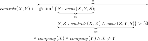 \begin{align}\begin{split}{\mathit{controls}}(X,Y) \leftarrow {}& \!\overbrace{\begin{aligned}[t]\mathrm{\#sum}^+ \{& \underbrace{S : {\mathit{owns}}(X,Y,S)}_{e_1}; \\& \underbrace{S,Z: {\mathit{controls}}(X,Z) \wedge {\mathit{owns}}(Z,Y,S)}_{e_2} \} > 50\end{aligned}}^{a} \\{} \wedge {}& {\mathit{company}}(X) \wedge {\mathit{company}}(Y) \wedge X \neq Y\end{split}\end{align}
containing aggregate a with elements $e_1$
and
$e_1$
and $e_2$
, into rules
$e_2$
, into rules $r_1$
to
$r_1$
to $r_4$
:
$r_4$
:
 \begin{align}\begin{split}{\mathit{controls}}(X,Y) \leftarrow {} & {\alpha_{a,r}(X,Y)}\\{} \wedge {} & {\mathit{company}}(X) \wedge {\mathit{company}}(Y) \wedge X \neq Y,\end{split}\end{align}
 \begin{align}\begin{split}{\epsilon_{a,r}(X,Y)} \leftarrow {} & 0 >50 \\{} \wedge {} & {\mathit{company}}(X) \wedge {\mathit{company}}(Y) \wedge X \neq Y,\end{split}\end{align}
 \begin{align}\begin{split}{\eta_{e_1,a,r}(S,X,Y)} \leftarrow {} & {\mathit{owns}}(X,Y,S) \\{} \wedge {} & {\mathit{company}}(X) \wedge {\mathit{company}}(Y) \wedge X \neq Y,\text{ and }\end{split}\end{align}
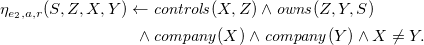 \begin{align}\begin{split}{\eta_{e_2,a,r}(S,Z,X,Y)} \leftarrow {} & {\mathit{controls}}(X,Z) \wedge {\mathit{owns}}(Z,Y,S)\\{} \wedge {} & {\mathit{company}}(X) \wedge {\mathit{company}}(Y) \wedge X \neq Y.\end{split}\end{align}
We have ${{P}^{\alpha}} = \{r_1\}$
,
${{P}^{\alpha}} = \{r_1\}$
, ${{P}^{\epsilon}} = \{ r_2 \}$
, and
${{P}^{\epsilon}} = \{ r_2 \}$
, and ${{P}^{\eta}} = \{ r_3, r_4 \}$
.
${{P}^{\eta}} = \{ r_3, r_4 \}$
.
This example illustrates how possible instantiations of aggregate elements are gathered via the rules in ${{P}^{\eta}}$
. Similarly, the rules in
${{P}^{\eta}}$
. Similarly, the rules in ${{P}^{\epsilon}}$
collect instantiations warranting that the result of applying aggregate functions to the empty set is in accord with the respective bound. In both cases, the relevant variable bindings are captured by the special head atoms of the rules. In turn, groups of corresponding instances of aggregate elements are used in Definition 20 to sanction the derivation of ground atoms of form (20). These atoms are ultimately replaced in
${{P}^{\epsilon}}$
collect instantiations warranting that the result of applying aggregate functions to the empty set is in accord with the respective bound. In both cases, the relevant variable bindings are captured by the special head atoms of the rules. In turn, groups of corresponding instances of aggregate elements are used in Definition 20 to sanction the derivation of ground atoms of form (20). These atoms are ultimately replaced in ${{P}^{\alpha}}$
with the original aggregate contents.
${{P}^{\alpha}}$
with the original aggregate contents.
We next define two functions gathering information from instances of rules in ${{P}^{\epsilon}}$
and
${{P}^{\epsilon}}$
and ${{P}^{\eta}}$
. In particular, we make precise how groups of aggregate element instances are obtained from ground rules in
${{P}^{\eta}}$
. In particular, we make precise how groups of aggregate element instances are obtained from ground rules in ${{P}^{\eta}}$
.
${{P}^{\eta}}$
.
Definition 18 Let P be an aggregate program, and ${{G}^{\epsilon}}$
and
${{G}^{\epsilon}}$
and ${{G}^{\eta}}$
be subsets of ground instances of rules in
${{G}^{\eta}}$
be subsets of ground instances of rules in ${{P}^{\epsilon}}$
and
${{P}^{\epsilon}}$
and ${{P}^{\eta}}$
, respectively. Furthermore, let a be an aggregate occurring in some rule
${{P}^{\eta}}$
, respectively. Furthermore, let a be an aggregate occurring in some rule $r \in P$
and
$r \in P$
and $\sigma$
be a substitution mapping the global variables in a to ground terms.
$\sigma$
be a substitution mapping the global variables in a to ground terms.
We define
 \begin{align*}{\epsilon_{r,a}({{G}^{\epsilon}},\sigma)} & = \bigcup_{g \in {{G}^{\epsilon}}} {\mathtt{Match}(r_a\sigma,g)},\end{align*}
where $r_a$
is a rule of form (21) for aggregate occurrence a, and
$r_a$
is a rule of form (21) for aggregate occurrence a, and
 \begin{align*}{\eta_{r,a}({{G}^{\eta}},\sigma)} & = \{ e\sigma\theta \mid g \in {{G}^{\eta}}, e \in E, \theta \in {\mathtt{Match}(r_e\sigma,g)} \},\end{align*}
where E are the aggregate elements of a and $r_e$
is a rule of form (22) for aggregate element occurrence e in a.
$r_e$
is a rule of form (22) for aggregate element occurrence e in a.
Given that $\sigma$
maps the global variables in a to ground terms,
$\sigma$
maps the global variables in a to ground terms, $r_a\sigma$
is ground whereas
$r_a\sigma$
is ground whereas $r_e\sigma$
may still contain local variables from a. The set
$r_e\sigma$
may still contain local variables from a. The set ${\epsilon_{r,a}({{G}^{\epsilon}},\sigma)}$
has an indicative nature: For an aggregate
${\epsilon_{r,a}({{G}^{\epsilon}},\sigma)}$
has an indicative nature: For an aggregate $a\sigma$
, it contains the identity substitution when the result of applying its aggregate function to the empty set is in accord with its bound, and it is empty otherwise. The construction of
$a\sigma$
, it contains the identity substitution when the result of applying its aggregate function to the empty set is in accord with its bound, and it is empty otherwise. The construction of ${\eta_{r,a}({{G}^{\eta}},\sigma)}$
goes one step further and reconstitutes all ground aggregate elements of
${\eta_{r,a}({{G}^{\eta}},\sigma)}$
goes one step further and reconstitutes all ground aggregate elements of $a\sigma$
from variable bindings obtained by rules in
$a\sigma$
from variable bindings obtained by rules in ${{G}^{\eta}}$
. Both functions play a central role below in defining the function
${{G}^{\eta}}$
. Both functions play a central role below in defining the function $\mathtt{Propagate}$
for deriving ground aggregate placeholders of form (20) from ground rules in
$\mathtt{Propagate}$
for deriving ground aggregate placeholders of form (20) from ground rules in ${{G}^{\epsilon}}$
and
${{G}^{\epsilon}}$
and ${{G}^{\eta}}$
.
${{G}^{\eta}}$
.
Example 22 We show how to extract aggregate elements from ground instances of rules (r3) and (r4) in Example 21.
Let ${{G}^{\epsilon}}$
be empty and
${{G}^{\epsilon}}$
be empty and ${{G}^{\eta}}$
be the program consisting of the following rules:
${{G}^{\eta}}$
be the program consisting of the following rules:
 \begin{align*}{\eta_{e_1,a,r}(60,c_1,c_2)} \leftarrow {} & {\mathit{owns}}(c_1,c_2,60)\\{} \wedge {} & {\mathit{company}}(c_1) \wedge {\mathit{company}}(c_2) \wedge c_1 \neq c_2,\\{\eta_{e_1,a,r}(20,c_1,c_3)} \leftarrow {} & {\mathit{owns}}(c_1,c_3,20)\\{} \wedge {} & {\mathit{company}}(c_1) \wedge {\mathit{company}}(c_3) \wedge c_1 \neq c_3,\\{\eta_{e_1,a,r}(35,c_2,c_3)} \leftarrow {} & {\mathit{owns}}(c_2,c_3,35)\\{} \wedge {} & {\mathit{company}}(c_2) \wedge {\mathit{company}}(c_3) \wedge c_2 \neq c_3,\\{\eta_{e_1,a,r}(51,c_3,c_4)} \leftarrow {} & {\mathit{owns}}(c_3,c_4,51)\\{} \wedge {} & {\mathit{company}}(c_3) \wedge {\mathit{company}}(c_4) \wedge c_3 \neq c_4,\text{ and }\\{\eta_{e_2,a,r}(35,c_2,c_1,c_3)} \leftarrow {} & {\mathit{controls}}(c_1,c_2) \wedge {\mathit{owns}}(c_2,c_3,35)\\{} \wedge {} & {\mathit{company}}(c_1) \wedge {\mathit{company}}(c_3) \wedge c_1 \neq c_3.\end{align*}
Clearly, we have ${\epsilon_{r,a}({{G}^{\epsilon}},\sigma)} = \emptyset$
for any substitution
${\epsilon_{r,a}({{G}^{\epsilon}},\sigma)} = \emptyset$
for any substitution $\sigma$
because
$\sigma$
because ${{G}^{\epsilon}} = \emptyset$
. This means that aggregate a can only be satisfied if at least one of its elements is satisfiable. In fact, we obtain non-empty sets
${{G}^{\epsilon}} = \emptyset$
. This means that aggregate a can only be satisfied if at least one of its elements is satisfiable. In fact, we obtain non-empty sets ${\eta_{r,a}({{G}^{\eta}},\sigma)}$
of ground aggregate elements for four substitutions
${\eta_{r,a}({{G}^{\eta}},\sigma)}$
of ground aggregate elements for four substitutions $\sigma$
:
$\sigma$
:
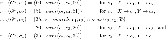 \begin{align*}{\eta_{r,a}({{G}^{\eta}},\sigma_1)} &= \{ 60: {\mathit{owns}}(c_1,c_2,60) \} & \text{ for } & \sigma_1: X \mapsto c_1, Y \mapsto c_2,\\{\eta_{r,a}({{G}^{\eta}},\sigma_2)} &= \{ 51: {\mathit{owns}}(c_3,c_4,51) \} & \text{ for } & \sigma_2: X \mapsto c_3, Y \mapsto c_4,\\{\eta_{r,a}({{G}^{\eta}},\sigma_3)} &= \rlap{$\{ 35, c_2: {\mathit{controls}}(c_1,c_2) \wedge {\mathit{owns}}(c_2,c_3,35)$;}\\&\phantom{{} = \{} 20: {\mathit{owns}}(c_1,c_3,20) \} & \text{ for } & \sigma_3: X \mapsto c_1, Y \mapsto c_3, \text{ and }\\{\eta_{r,a}({{G}^{\eta}},\sigma_4)} &= \{ 35: {\mathit{owns}}(c_2,c_3,35) \} & \text{ for } & \sigma_4: X \mapsto c_2, Y \mapsto c_3.\end{align*}
For capturing the result of grounding aggregates relative to groups of aggregate elements gathered via ${{P}^{\eta}}$
, we restrict their original translation to subsets of their ground elements. That is, while
${{P}^{\eta}}$
, we restrict their original translation to subsets of their ground elements. That is, while ${{\pi}(a)}$
and
${{\pi}(a)}$
and ${{{\pi}_{a}}(\cdot)}$
draw in Definition 9 on all instances of aggregate elements in a, their counterparts
${{{\pi}_{a}}(\cdot)}$
draw in Definition 9 on all instances of aggregate elements in a, their counterparts ${{{\pi}_{G}}(a)}$
and
${{{\pi}_{G}}(a)}$
and ${{{\pi}_{a,G}}(\cdot)}$
are restricted to a subset of such aggregate element instances:
Footnote 8
${{{\pi}_{a,G}}(\cdot)}$
are restricted to a subset of such aggregate element instances:
Footnote 8
Definition 19 Let a be a closed aggregate and of form (8), E be the set of its aggregate elements, and $G \subseteq {{\mathrm{Inst}}(E)}$
be a set of aggregate element instances.
$G \subseteq {{\mathrm{Inst}}(E)}$
be a set of aggregate element instances.
We define the translation ${{{\pi}_{G}}(a)}$
of a w.r.t. G as follows:
${{{\pi}_{G}}(a)}$
of a w.r.t. G as follows:
 \begin{align*}{{{\pi}_{G}}(a)} & = {\{ {{{\tau}(D)}}^\wedge \rightarrow {{{{\pi}_{a,G}}(D)}}^\vee \mid D \subseteq G, D \mathrel{\not\triangleright} a \}}^\wedge,\end{align*}
where
 \begin{align*}{{{\pi}_{a,G}}(D)} & = \{ {{{\tau}(C)}}^\wedge \mid C \subseteq G \setminus D, C \cup D \triangleright a \}.\end{align*}
As before, this translation maps aggregates, possibly including non-global variables, to a conjunction of (ground) ${\mathcal{R}}$
-rules. The resulting
${\mathcal{R}}$
-rules. The resulting ${\mathcal{R}}$
-formula is used below in the definition of functions
${\mathcal{R}}$
-formula is used below in the definition of functions $\mathtt{Propogate}$
and
$\mathtt{Propogate}$
and $\mathtt{Assemble}$
.
$\mathtt{Assemble}$
.
Example 23 We consider the four substitutions $\sigma_1$
to
$\sigma_1$
to $\sigma_4$
together with the sets
$\sigma_4$
together with the sets $G_1 = {\eta_{r,a}({{G}^{\eta}},\sigma_1)}$
to
$G_1 = {\eta_{r,a}({{G}^{\eta}},\sigma_1)}$
to $G_4 = {\eta_{r,a}({{G}^{\eta}},\sigma_4)}$
from Example 22 for aggregate a.
$G_4 = {\eta_{r,a}({{G}^{\eta}},\sigma_4)}$
from Example 22 for aggregate a.
Following the discussion after Proposition 24, we get the formulas
 \begin{align*}{{{\pi}_{G_1}}(a\sigma_1)} & = {\mathit{owns}}(c_1, c_2, 60),\\{{{\pi}_{G_2}}(a\sigma_2)} & = {\mathit{owns}}(c_3, c_4, 51),\\{{{\pi}_{G_3}}(a\sigma_3)} & = {\mathit{controls}}(c_1, c_2) \wedge {\mathit{owns}}(c_2,c_3,35) \wedge {\mathit{owns}}(c_1, c_3, 20)\text{, and }\\{{{\pi}_{G_4}}(a\sigma_4)} & = \bot.\end{align*}
The function $\mathtt{Propogate}$
yields a set of ground atoms of form (20) that are used in Algorithm 2 to ground rules having such placeholders among their body literals. Each such special atom is supported by a group of ground instances of its aggregate elements.
$\mathtt{Propogate}$
yields a set of ground atoms of form (20) that are used in Algorithm 2 to ground rules having such placeholders among their body literals. Each such special atom is supported by a group of ground instances of its aggregate elements.
Definition 20 Let P be an aggregate program, (I,J) be a four-valued interpretation, and ${{G}^{\epsilon}}$
and
${{G}^{\epsilon}}$
and ${{G}^{\eta}}$
be subsets of ground instances of rules in
${{G}^{\eta}}$
be subsets of ground instances of rules in ${{P}^{\epsilon}}$
and
${{P}^{\epsilon}}$
and ${{P}^{\eta}}$
, respectively.
${{P}^{\eta}}$
, respectively.
We define ${\mathtt{Propogate}_{P}^{I,J}({{G}^{\epsilon}},{{G}^{\eta}})}$
as the set of all atoms of form
${\mathtt{Propogate}_{P}^{I,J}({{G}^{\epsilon}},{{G}^{\eta}})}$
as the set of all atoms of form $\alpha\sigma$
such that
$\alpha\sigma$
such that ${\epsilon_{r,a}({{G}^{\epsilon}},\sigma)} \cup G \neq \emptyset$
and
${\epsilon_{r,a}({{G}^{\epsilon}},\sigma)} \cup G \neq \emptyset$
and $J \models {{{{\pi}_{G}}(a\sigma)}_{I}}$
with
$J \models {{{{\pi}_{G}}(a\sigma)}_{I}}$
with $G = {\eta_{r,a}({{G}^{\eta}},\sigma)}$
where
$G = {\eta_{r,a}({{G}^{\eta}},\sigma)}$
where $\alpha$
is an atom of form (20) for aggregate a in rule r and
$\alpha$
is an atom of form (20) for aggregate a in rule r and $\sigma$
is a ground substitution for r mapping all global variables in a to ground terms.
$\sigma$
is a ground substitution for r mapping all global variables in a to ground terms.
An atom $\alpha\sigma$
is only considered if
$\alpha\sigma$
is only considered if $\sigma$
warrants ground rules in
$\sigma$
warrants ground rules in ${{G}^{\epsilon}}$
or
${{G}^{\epsilon}}$
or ${{G}^{\eta}}$
, signaling that the application of
${{G}^{\eta}}$
, signaling that the application of $\alpha$
to the empty set is feasible when applying
$\alpha$
to the empty set is feasible when applying $\sigma$
or that there is a non-empty set of ground aggregate elements of
$\sigma$
or that there is a non-empty set of ground aggregate elements of $\alpha$
obtained after applying
$\alpha$
obtained after applying $\sigma$
, respectively. If this is the case, it is checked whether the set G of aggregate element instances warrants that
$\sigma$
, respectively. If this is the case, it is checked whether the set G of aggregate element instances warrants that ${{{\pi}_{G}}(a\sigma)}$
admits stable models between I and J.
${{{\pi}_{G}}(a\sigma)}$
admits stable models between I and J.
Example 24 We show how to propagate aggregates using the sets $G_1$
to
$G_1$
to $G_4$
and their associated formulas from Example 23. Suppose that
$G_4$
and their associated formulas from Example 23. Suppose that $I = J = F \cup \{ {\mathit{controls}}(c_1,c_2) \}$
using F from Example 20.
$I = J = F \cup \{ {\mathit{controls}}(c_1,c_2) \}$
using F from Example 20.
Observe that $J \models {{{{\pi}_{G_1}}(a\sigma_1)}_{I}}$
,
$J \models {{{{\pi}_{G_1}}(a\sigma_1)}_{I}}$
, $J \models {{{{\pi}_{G_2}}(a\sigma_2)}_{I}}$
,
$J \models {{{{\pi}_{G_2}}(a\sigma_2)}_{I}}$
, $J \models {{{{\pi}_{G_3}}(a\sigma_3)}_{I}}$
, and
$J \models {{{{\pi}_{G_3}}(a\sigma_3)}_{I}}$
, and $J \not\models {{{{\pi}_{G_4}}(a\sigma_4)}_{I}}$
. Thus, we get
$J \not\models {{{{\pi}_{G_4}}(a\sigma_4)}_{I}}$
. Thus, we get ${\mathtt{Propogate}_{P}^{I,J}({{G}^{\epsilon}},{{G}^{\eta}})} = \{ {\alpha_{a,r}(c_1,c_2)}, {\alpha_{a,r}(c_1,c_3)}, {\alpha_{a,r}(c_3,c_4)} \}$
.
${\mathtt{Propogate}_{P}^{I,J}({{G}^{\epsilon}},{{G}^{\eta}})} = \{ {\alpha_{a,r}(c_1,c_2)}, {\alpha_{a,r}(c_1,c_3)}, {\alpha_{a,r}(c_3,c_4)} \}$
.
The function $\mathtt{Assemble}$
yields an
$\mathtt{Assemble}$
yields an ${\mathcal{R}}$
-program in which aggregate placeholder atoms of form (20) have been replaced by their corresponding
${\mathcal{R}}$
-program in which aggregate placeholder atoms of form (20) have been replaced by their corresponding ${\mathcal{R}}$
-formulas.
${\mathcal{R}}$
-formulas.
Definition 21 Let P be an aggregate program, and ${{G}^{\alpha}}$
and
${{G}^{\alpha}}$
and ${{G}^{\eta}}$
be subsets of ground instances of rules in
${{G}^{\eta}}$
be subsets of ground instances of rules in ${{P}^{\alpha}}$
and
${{P}^{\alpha}}$
and ${{P}^{\eta}}$
, respectively.
${{P}^{\eta}}$
, respectively.
We define ${\mathtt{Assemble}({{G}^{\alpha}},{{G}^{\eta}})}$
as the
${\mathtt{Assemble}({{G}^{\alpha}},{{G}^{\eta}})}$
as the ${\mathcal{R}}$
-program obtained from
${\mathcal{R}}$
-program obtained from ${{G}^{\alpha}}$
by replacing
${{G}^{\alpha}}$
by replacing
-
all comparisons by
$\top$
and -
all atoms of form
$\alpha\sigma$
by the corresponding formulas
${{{\pi}_{G}}(a\sigma)}$
with
$G = {\eta_{r,a}({{G}^{\eta}},\sigma)}$
where
$\alpha$
is an atom of form (20) for aggregate a in rule r and
$\sigma$
is a ground substitution for r mapping all global variables in a to ground terms.


Example 25 We show how to assemble aggregates using the sets $G_1$
to
$G_1$
to $G_3$
for aggregate atoms that have been propagated in Example 24. Therefore, let
$G_3$
for aggregate atoms that have been propagated in Example 24. Therefore, let ${{G}^{\alpha}}$
be the program consisting of the following rules:
${{G}^{\alpha}}$
be the program consisting of the following rules:
 \begin{align*}{\mathit{controls}}(c_1,c_2) \leftarrow {} & {\alpha_{a,r}(c_1,c_2)} \wedge {} {\mathit{company}}(c_1) \wedge {\mathit{company}}(c_2) \wedge c_1 \neq c_2,\\{\mathit{controls}}(c_3,c_4) \leftarrow {} & {\alpha_{a,r}(c_3,c_4)} \wedge {} {\mathit{company}}(c_3) \wedge {\mathit{company}}(c_4) \wedge c_3 \neq c_4, \text{ and }\\{\mathit{controls}}(c_1,c_3) \leftarrow {} & {\alpha_{a,r}(c_1,c_3)} \wedge {} {\mathit{company}}(c_1) \wedge {\mathit{company}}(c_3) \wedge c_1 \neq c_3.\end{align*}
Then, program ${\mathtt{Assemble}({{G}^{\alpha}},{{G}^{\eta}})}$
consists of the following rules:
${\mathtt{Assemble}({{G}^{\alpha}},{{G}^{\eta}})}$
consists of the following rules:
 \begin{align*}{\mathit{controls}}(c_1,c_2) \leftarrow {} & {{{\pi}_{G_1}}(a\sigma_1)} \wedge {} {\mathit{company}}(c_1) \wedge {\mathit{company}}(c_2) \wedge \top,\\{\mathit{controls}}(c_3,c_4) \leftarrow {} & {{{\pi}_{G_2}}(a\sigma_2)} \wedge {} {\mathit{company}}(c_3) \wedge {\mathit{company}}(c_4) \wedge \top, \text{ and }\\{\mathit{controls}}(c_1,c_3) \leftarrow {} & {{{\pi}_{G_3}}(a\sigma_3)} \wedge {} {\mathit{company}}(c_1) \wedge {\mathit{company}}(c_3) \wedge \top.\end{align*}
The next result shows how a (non-ground) aggregate program P is transformed into a (ground) ${\mathcal{R}}$
-program
${\mathcal{R}}$
-program ${{{{\pi}_{J}}(P)}^{I,J}}$
in the context of certain and possible atoms (I,J) via the interplay of grounding
${{{{\pi}_{J}}(P)}^{I,J}}$
in the context of certain and possible atoms (I,J) via the interplay of grounding ${{P}^{\epsilon}}$
and
${{P}^{\epsilon}}$
and ${{P}^{\eta}}$
, deriving aggregate placeholders from their ground instances
${{P}^{\eta}}$
, deriving aggregate placeholders from their ground instances ${{G}^{\epsilon}}$
and
${{G}^{\epsilon}}$
and ${{G}^{\eta}}$
, and finally replacing them in
${{G}^{\eta}}$
, and finally replacing them in ${{G}^{\alpha}}$
by the original aggregates’ contents.
${{G}^{\alpha}}$
by the original aggregates’ contents.
Proposition 32 Let P be an aggregate program, (I,J) be a finite four-valued interpretation, ${{G}^{\epsilon}} = {{{\mathrm{Inst}}^{I,J}}({{P}^{\epsilon}})}$
,
${{G}^{\epsilon}} = {{{\mathrm{Inst}}^{I,J}}({{P}^{\epsilon}})}$
, ${{G}^{\eta}} = {{{\mathrm{Inst}}^{I,J}}({{P}^{\eta}})}$
,
${{G}^{\eta}} = {{{\mathrm{Inst}}^{I,J}}({{P}^{\eta}})}$
, ${\mathit{J\!A}} = {\mathtt{Propogate}_{P}^{I,J}({{G}^{\epsilon}},{{G}^{\eta}})}$
, and
${\mathit{J\!A}} = {\mathtt{Propogate}_{P}^{I,J}({{G}^{\epsilon}},{{G}^{\eta}})}$
, and ${{G}^{\alpha}} = {{{\mathrm{Inst}}^{I,J \cup {\mathit{J\!A}}}}({{P}^{\alpha}})}$
.
${{G}^{\alpha}} = {{{\mathrm{Inst}}^{I,J \cup {\mathit{J\!A}}}}({{P}^{\alpha}})}$
.
Then,
-
(a)
${\mathtt{Assemble}({{G}^{\alpha}},{{G}^{\eta}})} = {{{{\pi}_{J}}(P)}^{I,J}}$
and -
(b)
${H({{G}^{\alpha}})} = T_{{{{\pi}(P)}_{I}}}(J)$
.


Property (b) highlights the relation of the possible atoms contributed by ${{G}^{\alpha}}$
to a corresponding application of the immediate consequence operator. In fact, this is the first of three such relationships between grounding algorithms and consequence operators.
${{G}^{\alpha}}$
to a corresponding application of the immediate consequence operator. In fact, this is the first of three such relationships between grounding algorithms and consequence operators.
Algorithm 2: Grounding Components
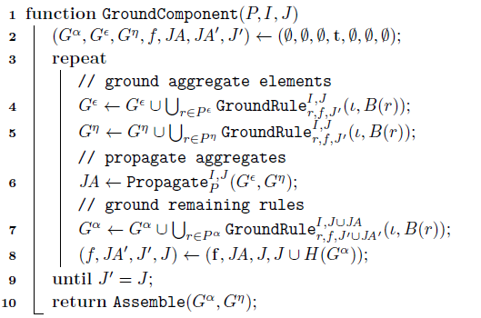
Let us now turn to grounding components of instantiation sequences in Algorithm 2. The function $\mathtt{GroundComponent}$
takes an aggregate program P along with two sets I and J of ground atoms. Intuitively, P is a component in a (refined) instantiation sequence and I and J form a four-valued interpretation (I,J) comprising the certain and possible atoms gathered while grounding previous components (although their roles get reversed in Algorithm 3). After variable initialization,
$\mathtt{GroundComponent}$
takes an aggregate program P along with two sets I and J of ground atoms. Intuitively, P is a component in a (refined) instantiation sequence and I and J form a four-valued interpretation (I,J) comprising the certain and possible atoms gathered while grounding previous components (although their roles get reversed in Algorithm 3). After variable initialization, $\mathtt{GroundComponent}$
loops over consecutive rule instantiations in
$\mathtt{GroundComponent}$
loops over consecutive rule instantiations in ${{P}^{\alpha}}$
,
${{P}^{\alpha}}$
, ${{P}^{\epsilon}}$
, and
${{P}^{\epsilon}}$
, and ${{P}^{\eta}}$
until no more possible atoms are obtained. In this case, it returns in Line 10 the
${{P}^{\eta}}$
until no more possible atoms are obtained. In this case, it returns in Line 10 the ${\mathcal{R}}$
-program obtained from
${\mathcal{R}}$
-program obtained from ${{G}^{\alpha}}$
by replacing all ground aggregate placeholders of form (20) with the
${{G}^{\alpha}}$
by replacing all ground aggregate placeholders of form (20) with the ${\mathcal{R}}$
-formula corresponding to the respective ground aggregate. The body of the loop can be divided into two parts: Lines 4–6 deal with aggregates and Lines 7 and 8 care about grounding the actual program. In more detail, Lines 4 and 5 instantiate programs
${\mathcal{R}}$
-formula corresponding to the respective ground aggregate. The body of the loop can be divided into two parts: Lines 4–6 deal with aggregates and Lines 7 and 8 care about grounding the actual program. In more detail, Lines 4 and 5 instantiate programs ${{P}^{\epsilon}}$
and
${{P}^{\epsilon}}$
and ${{P}^{\eta}}$
, whose ground instances,
${{P}^{\eta}}$
, whose ground instances, ${{G}^{\epsilon}}$
and
${{G}^{\epsilon}}$
and ${{G}^{\eta}}$
, are then used in Line 6 to derive ground instances of aggregate placeholders of form (20). The grounded placeholders are then added via variable
${{G}^{\eta}}$
, are then used in Line 6 to derive ground instances of aggregate placeholders of form (20). The grounded placeholders are then added via variable ${\mathit{J\!A}}$
to the possible atoms J when grounding the actual program
${\mathit{J\!A}}$
to the possible atoms J when grounding the actual program ${{P}^{\alpha}}$
in Line 7, where J’ and
${{P}^{\alpha}}$
in Line 7, where J’ and ${{\mathit{J\!A}}'}$
hold the previous value of J and
${{\mathit{J\!A}}'}$
hold the previous value of J and ${\mathit{J\!A}}$
, respectively. For the next iteration, J is augmented in Line 8 with all rule heads in
${\mathit{J\!A}}$
, respectively. For the next iteration, J is augmented in Line 8 with all rule heads in ${{G}^{\alpha}}$
and the flag f is set to false. Recall that the purpose of f is to ensure that initially all rules are grounded. In subsequent iterations, duplicates are omitted by setting the flag to false and filtering rules whose positive bodies are a subset of the atoms
${{G}^{\alpha}}$
and the flag f is set to false. Recall that the purpose of f is to ensure that initially all rules are grounded. In subsequent iterations, duplicates are omitted by setting the flag to false and filtering rules whose positive bodies are a subset of the atoms $J' \cup {{\mathit{J\!A}}'}$
used in previous iterations.
$J' \cup {{\mathit{J\!A}}'}$
used in previous iterations.
While the inner workings of Algorithm 2 follow the blueprint given by Proposition 32. its outer functionality boils down to applying the stable operator of the corresponding ground program in the context of the certain and possible atoms gathered so far.
Proposition 33 Let P be an aggregate program, $({\mathit{I\!{C}}},{\mathit{J\!{C}}})$
be a finite four-valued interpretation, and
$({\mathit{I\!{C}}},{\mathit{J\!{C}}})$
be a finite four-valued interpretation, and $J = {{{S}_{{{\pi}(P)}}^{{\mathit{J\!{C}}}}}({\mathit{I\!{C}}})}$
.
$J = {{{S}_{{{\pi}(P)}}^{{\mathit{J\!{C}}}}}({\mathit{I\!{C}}})}$
.
Then,
-
(a)
${\mathtt{GroundComponent}(P, {\mathit{I\!{C}}}, {\mathit{J\!{C}}})}$
terminates iff J is finite.

If J is finite, then
-
(a)
${\mathtt{GroundComponent}(P, {\mathit{I\!{C}}}, {\mathit{J\!{C}}})} = {{{{\pi}_{{\mathit{J\!{C}}} \cup J}}(P)}^{{\mathit{I\!{C}}}, {\mathit{J\!{C}}} \cup J}}$
and -
(b)
${H({\mathtt{GroundComponent}(P, {\mathit{I\!{C}}}, {\mathit{J\!{C}}})})} = J$
.


Algorithm 3: Grounding Programs
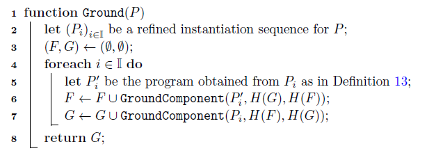
Finally, Algorithm 3 grounds an aggregate program by iterating over the components of one of its refined instantiation sequences. Just as Algorithm 2 reflects the application of a stable operator, function $\mathtt{GroundProgram}$
follows the definition of an approximate model when grounding a component (cf. Definition 13). At first, facts are computed in Line 6 by using the program stripped from rules being involved in a negative cycle overlapping with the present or subsequent components. The obtained head atoms are then used in Line 7 as certain context atoms when computing the ground version of the component at hand. The possible atoms are provided by the head atoms of the ground program built so far, and with roles reversed in Line 6. Accordingly, the whole iteration aligns with the approximate model of the chosen refined instantiation sequence (cf. Definition 14), as made precise next.
$\mathtt{GroundProgram}$
follows the definition of an approximate model when grounding a component (cf. Definition 13). At first, facts are computed in Line 6 by using the program stripped from rules being involved in a negative cycle overlapping with the present or subsequent components. The obtained head atoms are then used in Line 7 as certain context atoms when computing the ground version of the component at hand. The possible atoms are provided by the head atoms of the ground program built so far, and with roles reversed in Line 6. Accordingly, the whole iteration aligns with the approximate model of the chosen refined instantiation sequence (cf. Definition 14), as made precise next.
Our grounding algorithm computes implicitly the approximate model of the chosen instantiation sequence and outputs the corresponding ground program; it terminates whenever the approximate model is finite.
Theorem 34 Let P be an aggregate program, ${({{P}_{i}})}_{i \in \mathbb{I}}$
be a refined instantiation sequence for P, and
${({{P}_{i}})}_{i \in \mathbb{I}}$
be a refined instantiation sequence for P, and $({{\mathit{I\!{C}}}_{i}},{{\mathit{J\!{C}}}_{i}})$
and
$({{\mathit{I\!{C}}}_{i}},{{\mathit{J\!{C}}}_{i}})$
and $({I_{i}},{J_{i}})$
be defined as in Equations (15) and (16).
$({I_{i}},{J_{i}})$
be defined as in Equations (15) and (16).
If ${({{P}_{i}})}_{i \in \mathbb{I}}$
is selected by Algorithm 3 in Line 2, then we have that
${({{P}_{i}})}_{i \in \mathbb{I}}$
is selected by Algorithm 3 in Line 2, then we have that
-
(a) the call
${\mathtt{GroundProgram}(P)}$
terminates iff
${\mathit{AM}({({{P}_{i}})}_{i\in\mathbb{I}})}$
is finite, and -
(b) if
${\mathit{AM}({({{P}_{i}})}_{i\in\mathbb{I}})}$
is finite, then
${\mathtt{GroundProgram}(P)} = \bigcup_{i \in \mathbb{I}}{{{{\pi}_{{{\mathit{J\!{C}}}_{i}} \cup {J_{i}}}}({{P}_{i}})}^{({{\mathit{I\!{C}}}_{i}},{{\mathit{J\!{C}}}_{i}}) \sqcup ({I_{i}},{J_{i}})}}$
.


As already indicated by Theorem 29, grounding is governed by the series of consecutive approximate models $({I_{i}},{J_{i}})$
in (16) delineating the stable models of each ground program in a (refined) instantiation sequence. Whenever each of them is finite, we also obtain a finite grounding of the original program. Note that the entire ground program is composed of the ground programs of each component in the chosen instantiation sequence. Hence, different sequences may result in different overall ground programs.
$({I_{i}},{J_{i}})$
in (16) delineating the stable models of each ground program in a (refined) instantiation sequence. Whenever each of them is finite, we also obtain a finite grounding of the original program. Note that the entire ground program is composed of the ground programs of each component in the chosen instantiation sequence. Hence, different sequences may result in different overall ground programs.
Most importantly, our grounding machinery guarantees that an obtained finite ground program has the same stable models as the original non-ground program.
Corollary 35 (Main result) Let P be an aggregate program.
If ${\mathtt{GroundProgram}(P)}$
terminates, then P and
${\mathtt{GroundProgram}(P)}$
terminates, then P and ${\mathtt{GroundProgram}(P)}$
have the same well-founded and stable models.
${\mathtt{GroundProgram}(P)}$
have the same well-founded and stable models.
Example 26 The execution of the grounding algorithms on Example 19 is illustrated in Table 1. Each individual table depicts a call to $\mathtt{GroundComponent}$
where the header above the double line contains the (literals of the) rules to be grounded and the rows below trace how nested calls to
$\mathtt{GroundComponent}$
where the header above the double line contains the (literals of the) rules to be grounded and the rows below trace how nested calls to $\mathtt{GroundRule}$
proceed. The rules in the header contain the body literals in the order as they are selected by
$\mathtt{GroundRule}$
proceed. The rules in the header contain the body literals in the order as they are selected by $\mathtt{GroundRule}$
with the rule head as the last literal. Calls to
$\mathtt{GroundRule}$
with the rule head as the last literal. Calls to $\mathtt{GroundRule}$
are depicted with vertical lines and horizontal arrows. A vertical line represents the iteration of the loop in Lines 4–5. A horizontal arrow represents a recursive call to
$\mathtt{GroundRule}$
are depicted with vertical lines and horizontal arrows. A vertical line represents the iteration of the loop in Lines 4–5. A horizontal arrow represents a recursive call to $\mathtt{GroundRule}$
in Line 5. Each row in the table not marked with
$\mathtt{GroundRule}$
in Line 5. Each row in the table not marked with $\times$
corresponds to a ground instance as returned by
$\times$
corresponds to a ground instance as returned by $\mathtt{GroundRule}$
. Furthermore, because all components are stratified, we only show the first iteration of the loop in Lines 3–9 of Algorithm 2 as the second iteration does not produce any new ground instances.
$\mathtt{GroundRule}$
. Furthermore, because all components are stratified, we only show the first iteration of the loop in Lines 3–9 of Algorithm 2 as the second iteration does not produce any new ground instances.
Table 1. Grounding of components ${{P}_{5,1}}$
,
${{P}_{5,1}}$
, ${{P}_{5,2}}$
,
${{P}_{5,2}}$
, ${{P}_{6}}$
, and
${{P}_{6}}$
, and ${{P}_{7}}$
from Example 19 where
${{P}_{7}}$
from Example 19 where $\mathtt{GroundComponent}Short = \mathtt{GroundComponent}$

Grounding components ${{P}_{1}}$
to
${{P}_{1}}$
to ${{P}_{4}}$
results in the programs
${{P}_{4}}$
results in the programs $F = G = \{ u(1) \leftarrow \top, u(2) \leftarrow \top, v(2) \leftarrow \top, v(3) \leftarrow \top \}$
. Since grounding is driven by the sets of true and possible atoms, we focus on the interpretations
$F = G = \{ u(1) \leftarrow \top, u(2) \leftarrow \top, v(2) \leftarrow \top, v(3) \leftarrow \top \}$
. Since grounding is driven by the sets of true and possible atoms, we focus on the interpretations ${I_{i}}$
and
${I_{i}}$
and ${J_{i}}$
where i is a component index in the refined instantiation sequence. We start tracing the grounding starting with
${J_{i}}$
where i is a component index in the refined instantiation sequence. We start tracing the grounding starting with ${I_{4}} = {J_{4}} = \{ u(1), u(2), v(2), v(3) \}$
.
${I_{4}} = {J_{4}} = \{ u(1), u(2), v(2), v(3) \}$
.
The grounding of ${{P}_{5,1}}$
is depicted in Table 1a and 1b. We have
${{P}_{5,1}}$
is depicted in Table 1a and 1b. We have ${\mathcal{E}} = \{ b/1 \}$
because predicate
${\mathcal{E}} = \{ b/1 \}$
because predicate $b/1$
is used in the head of the rule in
$b/1$
is used in the head of the rule in ${{P}_{5,2}}$
. Thus,
${{P}_{5,2}}$
. Thus, ${\mathtt{GroundComponent}(\emptyset, {J_{4}}, {I_{4}})}$
in Line 6 returns the empty set because
${\mathtt{GroundComponent}(\emptyset, {J_{4}}, {I_{4}})}$
in Line 6 returns the empty set because ${{P}_{5,1}'} = \emptyset$
. We get
${{P}_{5,1}'} = \emptyset$
. We get ${I_{5,1}} = {I_{4}}$
. In the next line, the algorithm calls
${I_{5,1}} = {I_{4}}$
. In the next line, the algorithm calls ${\mathtt{GroundComponent}({{P}_{5,1}}, {I_{5,1}}, {J_{4}})}$
and we get
${\mathtt{GroundComponent}({{P}_{5,1}}, {I_{5,1}}, {J_{4}})}$
and we get ${J_{5,1}} = \{ p(1), p(2) \}$
. Note that at this point, it is not known that q(1) is not derivable and so the algorithm does not derive p(1) as a fact.
${J_{5,1}} = \{ p(1), p(2) \}$
. Note that at this point, it is not known that q(1) is not derivable and so the algorithm does not derive p(1) as a fact.
The grounding of ${{P}_{5,2}}$
is given in Table 1c and 1d. This time, we have
${{P}_{5,2}}$
is given in Table 1c and 1d. This time, we have ${\mathcal{E}} = \emptyset$
and
${\mathcal{E}} = \emptyset$
and ${{P}_{5,2}} = {{P}_{5,2}'}$
. Thus, the first call to
${{P}_{5,2}} = {{P}_{5,2}'}$
. Thus, the first call to $\mathtt{GroundRule}$
determines q(3) to be true while the second call additionally determines the possible atom q(2).
$\mathtt{GroundRule}$
determines q(3) to be true while the second call additionally determines the possible atom q(2).
The grounding of ${{P}_{6}}$
is illustrated in 1e and 1f. Note that we obtain that x is possible because p(1) was not determined to be true.
${{P}_{6}}$
is illustrated in 1e and 1f. Note that we obtain that x is possible because p(1) was not determined to be true.
The grounding of ${{P}_{7}}$
is depicted in 1g and 1h. Note that, unlike before, we obtain that y is false because q(3) was determined to be true.
${{P}_{7}}$
is depicted in 1g and 1h. Note that, unlike before, we obtain that y is false because q(3) was determined to be true.
Furthermore, observe that the choice of the refined instantiation sequence determines the output of the algorithm. In fact, swapping ${{P}_{5,1}}$
and
${{P}_{5,1}}$
and ${{P}_{5,2}}$
in the sequence would result in x being false and y being possible.
${{P}_{5,2}}$
in the sequence would result in x being false and y being possible.
To conclude, we give the grounding of the program as output by gringo in Table 2. The grounder furthermore omits the true body literals marked in green.
Table 2. Grounding of Example 19 as output by gringo

Example 27 We illustrate the grounding of aggregates on the company controls example in Example 10 using the grounding sequence ${{({{P}_{i}})}_{1 \leq i \leq 9}}$
and the set of facts F from Example 20. Observe that the grounding of components
${{({{P}_{i}})}_{1 \leq i \leq 9}}$
and the set of facts F from Example 20. Observe that the grounding of components ${{P}_{1}}$
to
${{P}_{1}}$
to ${{P}_{8}}$
produces the program
${{P}_{8}}$
produces the program $\{ a \leftarrow \top \mid a \in F \}$
. We focus on how component
$\{ a \leftarrow \top \mid a \in F \}$
. We focus on how component ${{P}_{9}}$
is grounded. Because there are no negative dependencies, the components
${{P}_{9}}$
is grounded. Because there are no negative dependencies, the components ${{P}_{9}}$
and
${{P}_{9}}$
and ${{P}_{9}'}$
in Line 5 of Algorithm 3 are equal. To ground component
${{P}_{9}'}$
in Line 5 of Algorithm 3 are equal. To ground component ${{P}_{9}}$
, we use the rewriting from Example 21.
${{P}_{9}}$
, we use the rewriting from Example 21.
The grounding of component ${{P}_{9}}$
is illustrated in Table 3, which follows the same conventions as in Example 26. Because the program is positive, the calls in Lines 6 and 7 in Algorithm 3 proceed in the same way and we depict only one of them. Furthermore, because this example involves a recursive rule with an aggregate, the header consists of five rows separated by dashed lines processed by Algorithm 2. The first row corresponds to
${{P}_{9}}$
is illustrated in Table 3, which follows the same conventions as in Example 26. Because the program is positive, the calls in Lines 6 and 7 in Algorithm 3 proceed in the same way and we depict only one of them. Furthermore, because this example involves a recursive rule with an aggregate, the header consists of five rows separated by dashed lines processed by Algorithm 2. The first row corresponds to ${{P}^{\epsilon}_{9}}$
grounded in Line 4, the second and third to
${{P}^{\epsilon}_{9}}$
grounded in Line 4, the second and third to ${{P}^{\eta}_{9}}$
grounded in Line 5, the fourth to aggregate propagation in Line 6, and the fifth to
${{P}^{\eta}_{9}}$
grounded in Line 5, the fourth to aggregate propagation in Line 6, and the fifth to ${{P}^{\alpha}_{9}}$
grounded in Line 7. After the header follow the iterations of the loop in Lines 3–9. Because the component is recursive, processing the component requires four iterations, which are separated by solid lines in the table. The right-hand side column of the table contains the iteration number and a number indicating which row in the header is processed. The row for aggregate propagation lists the aggregate atoms that have been propagated.
${{P}^{\alpha}_{9}}$
grounded in Line 7. After the header follow the iterations of the loop in Lines 3–9. Because the component is recursive, processing the component requires four iterations, which are separated by solid lines in the table. The right-hand side column of the table contains the iteration number and a number indicating which row in the header is processed. The row for aggregate propagation lists the aggregate atoms that have been propagated.
Table 3. Tracing grounding of component ${{P}_{9}}$
where
${{P}_{9}}$
where $c={\mathit{company}}$
,
$c={\mathit{company}}$
, $o={\mathit{owns}}$
, and
$o={\mathit{owns}}$
, and $s={\mathit{controls}}$

The grounding of rule $r_2$
in Row 1.1 does not produce any rule instances in any iteration because the comparison
$r_2$
in Row 1.1 does not produce any rule instances in any iteration because the comparison $0 > 50$
is false. By first selecting this literal when grounding the rule, the remaining rule body can be completely ignored. Actual systems implement heuristics to prioritize such literals. Next, in the grounding of rule
$0 > 50$
is false. By first selecting this literal when grounding the rule, the remaining rule body can be completely ignored. Actual systems implement heuristics to prioritize such literals. Next, in the grounding of rule $r_3$
in Row 1.2, direct shares given by facts over
$r_3$
in Row 1.2, direct shares given by facts over ${\mathit{owns}}/3$
are accumulated. Because the rule does not contain any recursive predicates, it only produces ground instances in the first iteration. Unlike this, rule
${\mathit{owns}}/3$
are accumulated. Because the rule does not contain any recursive predicates, it only produces ground instances in the first iteration. Unlike this, rule $r_4$
contains the recursive predicate
$r_4$
contains the recursive predicate ${\mathit{controls/2}}$
. It does not produce instances in the first iteration in Row 1.3 because there are no corresponding atoms yet. Next, aggregate propagation is triggered in Row 1.4, resulting in aggregate atoms
${\mathit{controls/2}}$
. It does not produce instances in the first iteration in Row 1.3 because there are no corresponding atoms yet. Next, aggregate propagation is triggered in Row 1.4, resulting in aggregate atoms ${\alpha_{a,r}(c_1,c_2)}$
and
${\alpha_{a,r}(c_1,c_2)}$
and ${\alpha_{a,r}(c_3,c_4)}$
, for which enough shares have been accumulated in Row 1.2. Note that this corresponds to the propagation of the sets
${\alpha_{a,r}(c_3,c_4)}$
, for which enough shares have been accumulated in Row 1.2. Note that this corresponds to the propagation of the sets $G_1$
and
$G_1$
and $G_2$
in Example 24. With these atoms, rule
$G_2$
in Example 24. With these atoms, rule $r_1$
is instantiated in Row 1.5, leading to new atoms over
$r_1$
is instantiated in Row 1.5, leading to new atoms over ${\mathit{controls}}/2$
. Observe that, by selecting atom
${\mathit{controls}}/2$
. Observe that, by selecting atom ${\alpha_{a,r}(X,Y)}$
first,
${\alpha_{a,r}(X,Y)}$
first, $\mathtt{GroundRule}$
can instantiate the rule without backtracking.
$\mathtt{GroundRule}$
can instantiate the rule without backtracking.
In the second iteration, the newly obtained atoms over predicate ${\mathit{controls}}/2$
yield atom
${\mathit{controls}}/2$
yield atom ${\eta_{e_1,a,r}(35,c_2,c_1,c_3)}$
in Row 2.3, which in turn leads to the aggregate atom
${\eta_{e_1,a,r}(35,c_2,c_1,c_3)}$
in Row 2.3, which in turn leads to the aggregate atom ${\alpha_{a,r}(c_1,c_3)}$
resulting in further instances of
${\alpha_{a,r}(c_1,c_3)}$
resulting in further instances of $r_4$
. Note that this corresponds to the propagation of the set
$r_4$
. Note that this corresponds to the propagation of the set $G_3$
in Example 24.
$G_3$
in Example 24.
The following iterations proceed in a similar fashion until no new atoms are accumulated and the grounding loop terminates. Note that the utilized selection strategy affects the amount of backtracking in rule instantiation. One particular strategy used in gringo is to prefer atoms over recursive predicates. If there is only one such atom, $\mathtt{GroundRule}$
can select this atom first and only has to consider newly derived atoms for instantiation. The table is made more compact by applying this strategy. Further techniques are available in the database literature (Ullman Reference Ullman1988) that also work in case of multiple atoms over recursive predicates.
$\mathtt{GroundRule}$
can select this atom first and only has to consider newly derived atoms for instantiation. The table is made more compact by applying this strategy. Further techniques are available in the database literature (Ullman Reference Ullman1988) that also work in case of multiple atoms over recursive predicates.
To conclude, we give the ground rules as output by a grounder like gringo in Table 4. We omit the translation of aggregates because its main objective is to show correctness of the algorithms. Solvers like clasp implement translations or even native handling of aggregates geared toward efficient solving (Gebser et al. Reference Gebser, Kaminski, Kaufmann and Schaub2009). Since our example program is positive, gringo is even able to completely evaluate the rules to facts omitting true literals from rule bodies marked in green.
Table 4. Grounding of the company controls problem from Example 10 as output by gringo

7 Refinements
Up to now, we were primarily concerned by characterizing the theoretical and algorithmic cornerstones of grounding. This section refines these concepts by further detailing aggregate propagation, algorithm specifics, and the treatment of language constructs from gringo’s input language.
7.1 Aggregate propagation
We used in Section 6 the relative translation of aggregates for propagation, namely, formula ${{{\pi}_{G}}(a\sigma)}$
in Definition 20, to check whether an aggregate is satisfiable. In this section, we identify several aggregate specific properties that allow us to implement more efficient algorithms to perform this check.
${{{\pi}_{G}}(a\sigma)}$
in Definition 20, to check whether an aggregate is satisfiable. In this section, we identify several aggregate specific properties that allow us to implement more efficient algorithms to perform this check.
To begin with, we establish some properties that greatly simplify the treatment of (arbitrary) monotone or antimonotone aggregates.
We have already seen in Proposition 24 that ${{{\pi}(a)}_{I}}$
is classically equivalent to
${{{\pi}(a)}_{I}}$
is classically equivalent to ${{\pi}(a)}$
for any closed aggregate a and two-valued interpretation I. Here is its counterpart for antimonotone aggregates.
${{\pi}(a)}$
for any closed aggregate a and two-valued interpretation I. Here is its counterpart for antimonotone aggregates.
Proposition 36 Let a be a closed aggregate.
If a is antimonotone, then ${{{\pi}(a)}_{I}}$
is classically equivalent to
${{{\pi}(a)}_{I}}$
is classically equivalent to $\top$
if
$\top$
if $I \models {{\pi}(a)}$
and
$I \models {{\pi}(a)}$
and $\bot$
otherwise for any two-valued interpretation I.
$\bot$
otherwise for any two-valued interpretation I.
Example 28 In Example 24, we check whether the interpretation J satisfies the formulas ${{{{\pi}_{G_1}}(a\sigma_1)}_{I}}$
to
${{{{\pi}_{G_1}}(a\sigma_1)}_{I}}$
to ${{{{\pi}_{G_4}}(a\sigma_4)}_{I}}$
.
${{{{\pi}_{G_4}}(a\sigma_4)}_{I}}$
.
Using Proposition 24, this boils down to checking $\sum_{e \in G_i, J \models {B(e)}}{H(e)} > 50$
for each
$\sum_{e \in G_i, J \models {B(e)}}{H(e)} > 50$
for each $1 \leq i \leq 4$
. We get
$1 \leq i \leq 4$
. We get $60 > 50$
,
$60 > 50$
, $51 > 50$
,
$51 > 50$
, $55 > 50$
, and
$55 > 50$
, and $35 \not> 50$
for each
$35 \not> 50$
for each $G_i$
, which agrees with checking
$G_i$
, which agrees with checking $J \models {{{{\pi}_{G_i}}(a\sigma_i)}_{I}}$
.
$J \models {{{{\pi}_{G_i}}(a\sigma_i)}_{I}}$
.
An actual implementation can maintain a counter for the current value of the sum for each closed aggregate instance, which can be updated incrementally and compared with the bound as new instances of aggregate elements are grounded.
Next, we see that such counter based implementations are also possible #sum aggregates using the $<$
,
$<$
, $\leq$
,
$\leq$
, $>$
, or
$>$
, or $\geq$
relations. We restrict our attention to finite interpretations because Proposition 37 is intended to give an idea on how to implement an actual propagation algorithm for aggregates (infinite interpretations would add more special cases). Furthermore, we just consider the case that the bound is an integer here; the aggregate is constant for any other ground term.
$\geq$
relations. We restrict our attention to finite interpretations because Proposition 37 is intended to give an idea on how to implement an actual propagation algorithm for aggregates (infinite interpretations would add more special cases). Furthermore, we just consider the case that the bound is an integer here; the aggregate is constant for any other ground term.
Proposition 37 Let I be a finite two-valued interpretation, E be a set of aggregate elements, and b be an integer.
For $T = {H(\{e \in {{\mathrm{Inst}}(E)} \mid I \models {B(e)}\})}$
, we get
$T = {H(\{e \in {{\mathrm{Inst}}(E)} \mid I \models {B(e)}\})}$
, we get
-
(a)
${{{\pi}({\mathrm{\#sum} \{ E \} \succ b})}_{I}}$
is classically equivalent to
${{\pi}({{\mathrm{\#sum}^+} \{ E \} \succ b'})}$
with
${\succ} \in \{ {\geq}, {>} \}$
and
$b' = b - {\mathrm{\#sum}^-}(T)$
, and -
(b)
${{{\pi}({\mathrm{\#sum} \{ E \} \prec b})}_{I}}$
is classically equivalent to
${{\pi}({{\mathrm{\#sum}^-} \{ E \} \prec b'})}$
with
${\prec} \in \{ {\leq}, {<} \}$
and
$b' = b - {\mathrm{\#sum}^+}(T)$
.


The remaining propositions identify properties that can be exploited when propagating aggregates over the $=$
and
$=$
and $\neq$
relations.
$\neq$
relations.
Proposition 38 Let I be a two-valued interpretation, E be a set of aggregate elements, and b be a ground term.
We get the following properties: enumi enumi
-
(a)
${{{\pi}({f \{ E \} < b})}_{I}} \vee {{{\pi}({f \{ E \} > b})}_{I}}\text{ implies }{{{\pi}({f \{ E \} \neq b})}_{I}}$
, and -
(b)
${{{\pi}({f \{ E \} = b})}_{I}}\text{ implies }{{{\pi}({f \{ E \} \leq b})}_{I}} \wedge {{{\pi}({f \{ E \} \geq b})}_{I}}$
.


The following proposition identifies special cases when the implications in Proposition 38 are equivalences. Another interesting aspect of this proposition is that we can actually replace #sum aggregates over $=$
and
$=$
and $\neq$
with a conjunction or disjunction, respectively, at the expense of calculating a less precise approximate model. The conjunction is even strongly equivalent to the original aggregate under Ferraris’ semantics but not the disjunction.
$\neq$
with a conjunction or disjunction, respectively, at the expense of calculating a less precise approximate model. The conjunction is even strongly equivalent to the original aggregate under Ferraris’ semantics but not the disjunction.
Proposition 39 Let I and J be two-valued interpretations, f be an aggregate function among #count, ${\mathrm{\#sum}^+}$
,
${\mathrm{\#sum}^+}$
, ${\mathrm{\#sum}^-}$
or #sum, E be a set of aggregate elements, and b be an integer.
${\mathrm{\#sum}^-}$
or #sum, E be a set of aggregate elements, and b be an integer.
We get the following properties: enumi enumi
-
(a) for
$I \subseteq J$
, we have
$J \models {{{\pi}({f \{ E \} < b})}_{I}} \vee {{{\pi}({f \{ E \} > b})}_{I}}$
iff
$J \models {{{\pi}({f \{ E \} \neq b})}_{I}}$
, and -
(b) for
$J \subseteq I$
, we have
$J \models {{{\pi}({f \{ E \} = b})}_{I}}$
iff
$J \models {{{\pi}({f \{ E \} \leq b})}_{I}} \wedge {{{\pi}({f \{ E \} \geq b})}_{I}}$
.


The following proposition shows that full propagation of #sum, ${\mathrm{\#sum}^+}$
, or
${\mathrm{\#sum}^+}$
, or ${\mathrm{\#sum}^-}$
aggregates over relations
${\mathrm{\#sum}^-}$
aggregates over relations $=$
and
$=$
and $\neq$
involves solving the subset sum problem (Martello and Toth Reference Martello and Toth1990). We assume that we propagate w.r.t. some polynomial number of aggregate elements. Propagating possible atoms when using the
$\neq$
involves solving the subset sum problem (Martello and Toth Reference Martello and Toth1990). We assume that we propagate w.r.t. some polynomial number of aggregate elements. Propagating possible atoms when using the $=$
relation, that is, when
$=$
relation, that is, when $I \subseteq J$
, involves deciding an NP problem and propagating certain atoms when using the
$I \subseteq J$
, involves deciding an NP problem and propagating certain atoms when using the $\neq$
relation, that is, when
$\neq$
relation, that is, when $J \subseteq I$
, involves deciding a co-NP problem.
Footnote 9
Note that the decision problem for #count aggregates is polynomial, though.
$J \subseteq I$
, involves deciding a co-NP problem.
Footnote 9
Note that the decision problem for #count aggregates is polynomial, though.
Proposition 40 Let I and J be finite two-valued interpretations, f be an aggregate function, E be a set of aggregate elements, and b be a ground term.
For $T_I = \{ {H(e)} \mid e \in {{\mathrm{Inst}}(E)}, I \models {B(e)} \}$
and
$T_I = \{ {H(e)} \mid e \in {{\mathrm{Inst}}(E)}, I \models {B(e)} \}$
and $T_J = \{ {H(e)} \mid e \in {{\mathrm{Inst}}(E)}, J \models {B(e)} \}$
, we get the following properties:
$T_J = \{ {H(e)} \mid e \in {{\mathrm{Inst}}(E)}, J \models {B(e)} \}$
, we get the following properties:
-
(a) for
$J \subseteq I$
, we have
$J \models {{{\pi}({f \{ E \} \neq b})}_{I}}$
iff there is no set
$X \subseteq T_I$
such that
$f(X \cup T_J) = b$
, and -
(b) for
$I \subseteq J$
, we have
$J \models {{{\pi}({f \{ E \} = b})}_{I}}$
and iff there is a set
$X \subseteq T_J$
such that
$f(X \cup T_I) = b$
.


7.2 Algorithmic refinements
The calls in Lines 6 and 7 in Algorithm 3 can sometimes be combined to calculate certain and possible atoms simultaneously. This can be done whenever a component does not contain recursive predicates. In this case, it is sufficient to just calculate possible atoms along with rule instances in Line 7 augmenting Algorithm 1 with an additional check to detect whether a rule instance produces a certain atom. Observe that this condition applies to all stratified components but can also apply to components depending on unstratified components. In fact, typical programs following the generate, define, and test methodology (Lifschitz Reference Lifschitz2002; Niemelä Reference Niemelä2008) of ASP, where the generate part uses choice rules (Simons et al. Reference Simons, Niemelä and Soininen2002) (see below), do not contain unstratified negation at all. When a grounder is combined with a solver built to store rules and perform inferences, one can optimize for the case that there are no negative recursive predicates in a component. In this case, it is sufficient to compute possible atoms along with their rule instances and leave the computation of certain atoms to the solver. Finally, note that gringo currently does not separate the calculation of certain and possible atoms at the expense of computing a less precise approximate model and possibly additional rule instances.
Example 29 For the following example, gringo computes atom p(4) as unknown but the algorithms in Section 6 identify it as true.

When grounding the last rule, gringo determines p(4) to be possible in the first iteration because p(1) is unknown at this point. In the second iteration, it detects that p(1) is a fact but does not use it for grounding again. If there were further rules depending negatively on predicate $p/1$
, inapplicable rules might appear in gringo’s output.
$p/1$
, inapplicable rules might appear in gringo’s output.
Another observation is that the loop in Algorithm 2 does not produce further rule instances in a second iteration for components without recursive predicates. Gringo maintains an index (Garcia-Molina et al. Reference Garcia-Molina, Ullman and Widom2009) for each positive body literal to speed up matching of literals; whenever none of these indexes, used in rules of the component at hand, are updated, further iterations can be skipped.
Just like dlv’s grounder, gringo adapts algorithms for semi-naive evaluation from the field of databases. In particular, it works best on linear programs (Abiteboul et al. Reference Abiteboul, Hull and Vianu1995), having at most one positive literal occurrence over a recursive predicate in a rule body. The program in Example 10 for the company controls problem is such a linear program because ${\mathit{controls}}/2$
is the only recursive predicate. Algorithm 1 can easily be adapted to efficiently ground linear programs by making sure that the recursive positive literal is selected first. We then only have to consider matches that induce atoms not already used for instantiations in previous iterations of the loop in Algorithm 2 to reduce the amount of backtracking to find rule instances. In fact, the order in which literals are selected in Line 3 is crucial for the performance of Algorithm 1. Gringo uses an adaptation of the selection heuristics presented by Leone et al. (Reference Leone, Perri and Scarcello2001) that additionally takes into account recursive predicates and terms with function symbols.
${\mathit{controls}}/2$
is the only recursive predicate. Algorithm 1 can easily be adapted to efficiently ground linear programs by making sure that the recursive positive literal is selected first. We then only have to consider matches that induce atoms not already used for instantiations in previous iterations of the loop in Algorithm 2 to reduce the amount of backtracking to find rule instances. In fact, the order in which literals are selected in Line 3 is crucial for the performance of Algorithm 1. Gringo uses an adaptation of the selection heuristics presented by Leone et al. (Reference Leone, Perri and Scarcello2001) that additionally takes into account recursive predicates and terms with function symbols.
To avoid unnecessary backtracking when grounding general logic programs, gringo instantiates rules using an algorithm similar to the improved semi-naive evaluation with optimizations for linear rules (Abiteboul et al. Reference Abiteboul, Hull and Vianu1995).
7.3 Capturing gringo’s input language
We presented aggregate programs where rule heads are simple atoms. Beyond that, gringo’s input language offers more elaborate language constructs to ease modeling.
A prominent such construct are so-called choice rules (Simons et al. Reference Simons, Niemelä and Soininen2002). Syntactically, one-element choice rules have the form $\{a\}\leftarrow B$
, where a is an atom and B a body. Semantically, such a rule amounts to
$\{a\}\leftarrow B$
, where a is an atom and B a body. Semantically, such a rule amounts to $a\vee\neg a\leftarrow B$
or equivalently
$a\vee\neg a\leftarrow B$
or equivalently $a\leftarrow \neg\neg a\wedge B$
. We can easily add support for grounding choice rules, that is, rules where the head is not a plain atom but an atom marked as a choice, by discarding choice rules when calculating certain atoms and treating them like normal rules when grounding possible atoms. A translation that allows for supporting head aggregates using a translation to aggregate rules and choice rules is given by Gebser et al. (Reference Gebser, Harrison, Kaminski, Lifschitz and Schaub2015a). Note that gringo implements further refinements to omit deriving head atoms if a head aggregate cannot be satisfied.
$a\leftarrow \neg\neg a\wedge B$
. We can easily add support for grounding choice rules, that is, rules where the head is not a plain atom but an atom marked as a choice, by discarding choice rules when calculating certain atoms and treating them like normal rules when grounding possible atoms. A translation that allows for supporting head aggregates using a translation to aggregate rules and choice rules is given by Gebser et al. (Reference Gebser, Harrison, Kaminski, Lifschitz and Schaub2015a). Note that gringo implements further refinements to omit deriving head atoms if a head aggregate cannot be satisfied.
Another language feature that can be instantiated in a similar fashion as body aggregates are conditional literals. Gringo adapts the rewriting and propagation of body aggregates to also support grounding of conditional literals.
Yet another important language feature are disjunctions in the head of rules (Gelfond and Lifschitz Reference Gelfond and Lifschitz1991). As disjunctive logic programs, aggregate programs allow us to solve problems from the second level of the polynomial hierarchy. In fact, using Łukasiewicz’ theorem (Lukasiewicz Reference Lukasiewicz1941), we can write a disjunctive rule of form
 \begin{align*}a \vee b & \leftarrow B\end{align*}
as the shifted strongly equivalent ${\mathcal{R}}$
-program:
${\mathcal{R}}$
-program:
 \begin{align*}a & \leftarrow (b \rightarrow a)\wedge B\\b & \leftarrow (a \rightarrow b)\wedge B.\end{align*}
We can use this as a template to design grounding algorithms for disjunctive programs. In fact, gringo calculates the same approximate model for the disjunctive rule and the shifted program.
The usage of negation as failure is restricted in ${\mathcal{R}}$
-programs. Note that any occurrence of a negated literal l in a rule body can be replaced by an auxiliary atom a adding rule
${\mathcal{R}}$
-programs. Note that any occurrence of a negated literal l in a rule body can be replaced by an auxiliary atom a adding rule $a \leftarrow l$
to the program. The resulting program preserves the stable models modulo the auxiliary atoms. This translation can serve as a template for double negation or negation in aggregate elements as supported by gringo.
$a \leftarrow l$
to the program. The resulting program preserves the stable models modulo the auxiliary atoms. This translation can serve as a template for double negation or negation in aggregate elements as supported by gringo.
Integrity constraints are a straightforward extension of logic programs. They can be grounded just like normal rules deriving an auxiliary atom that stands for $\bot$
. Grounding can be stopped whenever the auxiliary atom is derived as certain. Integrity constraints also allow for supporting negated head atoms, which can be shifted to rule bodies (Janhunen Reference Janhunen2001) resulting in integrity constraints, and then treated like negation in rule bodies.
$\bot$
. Grounding can be stopped whenever the auxiliary atom is derived as certain. Integrity constraints also allow for supporting negated head atoms, which can be shifted to rule bodies (Janhunen Reference Janhunen2001) resulting in integrity constraints, and then treated like negation in rule bodies.
A frequently used convenience feature of gringo are term pools (Gebser et al. Reference Gebser, Harrison, Kaminski, Lifschitz and Schaub2015a; Gebser et al. Reference Gebser, Kaminski, Kaufmann, Lindauer, Ostrowski, Romero, Schaub and Thiele2015b). The grounder handles them by removing them in a rewriting step. For example, a rule of form
 \begin{align*}h(X;Y,Z) & \leftarrow p(X;Y), q(Z)\end{align*}
is factored out into the following rules:
 \begin{align*}h(X,Z) & \leftarrow p(X), q(Z)\\[2pt]h(X,Z) & \leftarrow p(Y), q(Z)\\[2pt]h(Y,Z) & \leftarrow p(X), q(Z)\\[2pt]h(Y,Z) & \leftarrow p(Y), q(Z).\end{align*}
We can then apply the grounding algorithms developed in Section 6.
To deal with variables ranging over integers, gringo supports interval terms (Gebser et al. Reference Gebser, Harrison, Kaminski, Lifschitz and Schaub2015a; Gebser et al. Reference Gebser, Kaminski, Kaufmann, Lindauer, Ostrowski, Romero, Schaub and Thiele2015b). Such terms are handled by a translation to inbuilt range predicates. For example the program
 \begin{align*}h(l..u) &\end{align*}
for terms l and u is rewritten into
 \begin{align*}h(A) & \leftarrow {\mathit{rng}}(A,l,u)\end{align*}
by introducing auxiliary variable A and range atom ${\mathit{rng}}(A,l,u)$
. The range atom provides matches including all substitutions that assign integer values between l and u to A. Special care has to be taken regarding rule safety, the range atom can only provide bindings for variable A but needs variables in the terms l and u to be provided elsewhere.
${\mathit{rng}}(A,l,u)$
. The range atom provides matches including all substitutions that assign integer values between l and u to A. Special care has to be taken regarding rule safety, the range atom can only provide bindings for variable A but needs variables in the terms l and u to be provided elsewhere.
A common feature used when writing logic programs are terms involving arithmetic expressions and assignments. Both influence which rules are considered safe by the grounder. For example, the rule
 \begin{align*}h(X,Y) & \leftarrow p(X+Y,Y) \wedge X = Y + Y\end{align*}
is rewritten into
 \begin{align*}h(X,Y) & \leftarrow p(A,Y) \wedge X = Y + Y \wedge A = X + Y\end{align*}
by introducing auxiliary variable A. The rule is safe because we can match the literals in the order as given in the rewritten rule. The comparison $X = Y + Y$
extends the substitution with an assignment for X and the last comparison serves as a test. Gringo does not try to solve complicated equations but supports simple forms like the one given above.
$X = Y + Y$
extends the substitution with an assignment for X and the last comparison serves as a test. Gringo does not try to solve complicated equations but supports simple forms like the one given above.
Last but not least, gringo does not just support terms in assignments but it also supports aggregates in assignments. To handle such kind of aggregates, the rewriting and propagation of aggregates has to be extended. This is achieved by adding an additional variable to aggregate replacement atoms (20), which is assigned by propagation. For example, the rule
 \begin{align*}\rlap{$\underbrace{h(X,Y) \leftarrow q(X) \wedge \overbrace{Y = \mathrm{\#sum} \{ Z: p(X,Z) \}}^a}_r$}\phantom{h(X,Y)} & \phantom{\leftarrow q(X) \wedge \overbrace{Y = \mathrm{\#sum} \{ Z: p(X,Z) \}}^a}\end{align*}
is rewritten into
 \begin{align*}{\epsilon_{a,r}(X)} & \leftarrow q(X)\\{\eta_{e,a,r}(Z,X)} & \leftarrow p(X,Z) \wedge q(X)\\h(X,Y) & \leftarrow {\alpha_{a,r}(X,Y)}.\end{align*}
Aggregate elements are grounded as before but values for variable Y are computed during aggregate propagation. In case of multiple assignment aggregates, additional care has to to be taken during the rewriting to ensure that the rewritten rules are safe.
8 Related work
This section aims at inserting our contributions into the literature, starting with theoretical aspects over algorithmic ones to implementations.
Splitting for infinitary formulas has been introduced by Harrison and Lifschitz (Reference Harrison and Lifschitz2016) generalizing results of Janhunen et al. (Reference Janhunen, Oikarinen, Tompits and Woltran2007) and Ferraris et al. (Reference Ferraris, Lee, Lifschitz and Palla2009). To this end, the concept of an A-stable model is introduced (Harrison and Lifschitz Reference Harrison and Lifschitz2016). We obtain the following relationship between our definition of a stable model relative to a set ${\mathit{I\!{C}}}$
and A-stable models: For an
${\mathit{I\!{C}}}$
and A-stable models: For an ${\mathcal{N}}$
-program P, we have that if X is a stable model of P relative to
${\mathcal{N}}$
-program P, we have that if X is a stable model of P relative to ${\mathit{I\!{C}}}$
, then
${\mathit{I\!{C}}}$
, then $X \cup {\mathit{I\!{C}}}$
is an
$X \cup {\mathit{I\!{C}}}$
is an $(\mathcal{A}\setminus{\mathit{I\!{C}}})$
-stable model of P. Similarly, we get that if X is an A-stable model of P, then
$(\mathcal{A}\setminus{\mathit{I\!{C}}})$
-stable model of P. Similarly, we get that if X is an A-stable model of P, then ${{{S}_{P}^{X \setminus A}}(X)}$
is a stable model of P relative to
${{{S}_{P}^{X \setminus A}}(X)}$
is a stable model of P relative to $X \setminus A$
. The difference between the two concepts is that we fix atoms
$X \setminus A$
. The difference between the two concepts is that we fix atoms ${\mathit{I\!{C}}}$
in our definition while A-stable models allow for assigning arbitrary truth values to atoms in
${\mathit{I\!{C}}}$
in our definition while A-stable models allow for assigning arbitrary truth values to atoms in $\mathcal{A} \setminus A$
(Harrison and Lifschitz (Reference Harrison and Lifschitz2016), Proposition 1). With this, let us compare our handling of program sequences to symmetric splitting (Harrison and Lifschitz Reference Harrison and Lifschitz2016). Let
$\mathcal{A} \setminus A$
(Harrison and Lifschitz (Reference Harrison and Lifschitz2016), Proposition 1). With this, let us compare our handling of program sequences to symmetric splitting (Harrison and Lifschitz Reference Harrison and Lifschitz2016). Let ${{{({{P}_{i}})}_{i \in \mathbb{I}}}}$
be a refined instantiation sequence of aggregate program P, and
${{{({{P}_{i}})}_{i \in \mathbb{I}}}}$
be a refined instantiation sequence of aggregate program P, and $F = \bigcup_{i < j} {{\pi}({{P}_{i}})}$
and
$F = \bigcup_{i < j} {{\pi}({{P}_{i}})}$
and $G = \bigcup_{i \geq j} {{\pi}({{P}_{i}})} $
for some
$G = \bigcup_{i \geq j} {{\pi}({{P}_{i}})} $
for some $j \in \mathbb{I}$
such that
$j \in \mathbb{I}$
such that ${H(F)} \neq {H(G)}$
. We can use the infinitary splitting theorem of Harrison and Lifschitz (Reference Harrison and Lifschitz2016) to calculate the stable model of
${H(F)} \neq {H(G)}$
. We can use the infinitary splitting theorem of Harrison and Lifschitz (Reference Harrison and Lifschitz2016) to calculate the stable model of $F^\wedge \wedge G^\wedge$
through the H(F)- and
$F^\wedge \wedge G^\wedge$
through the H(F)- and $\mathcal{A} \setminus {H(F)}$
-stable models of
$\mathcal{A} \setminus {H(F)}$
-stable models of $F^\wedge \wedge G^\wedge$
. Observe that instantiation sequences do not permit positive recursion between their components and infinite walks are impossible because an aggregate program consists of finitely many rules inducing a finite dependency graph. Note that we additionally require the condition
$F^\wedge \wedge G^\wedge$
. Observe that instantiation sequences do not permit positive recursion between their components and infinite walks are impossible because an aggregate program consists of finitely many rules inducing a finite dependency graph. Note that we additionally require the condition ${H(F)} \neq {H(G)}$
because components can be split even if their head atoms overlap. Such a split can only occur if overlapping head atoms in preceding components are not involved in positive recursion.
${H(F)} \neq {H(G)}$
because components can be split even if their head atoms overlap. Such a split can only occur if overlapping head atoms in preceding components are not involved in positive recursion.
Next, let us relate our operators to the ones defined by Truszczyński (Reference Truszczyński2012). First of all, it is worthwhile to realize that the motivation of Truszczyński (Reference Truszczyński2012) is to conceive operators mimicking model expansion in id-logic by adding certain atoms. More precisely, let $\mathit{\Phi}$
,
$\mathit{\Phi}$
, $\mathit{St}$
, and
$\mathit{St}$
, and $\mathit{Wf}$
stand for the versions of the Fitting, stable, and well-founded operators defined by Truszczyński (Reference Truszczyński2012). Then, we get the following relations to the operators defined in the previous sections:
$\mathit{Wf}$
stand for the versions of the Fitting, stable, and well-founded operators defined by Truszczyński (Reference Truszczyński2012). Then, we get the following relations to the operators defined in the previous sections:
 \begin{align*}{\mathit{St}_{P,{\mathit{I\!{C}}}}({J})}& = {\mathit{lfp}({{\mathit{\Phi}_{P,{\mathit{I\!{C}}}}({\cdot,J})}})}\\& = {\mathit{lfp}({T^{{\mathit{I\!{C}}}}_{P_J}})} \cup {\mathit{I\!{C}}}\\& = {{{S}_{P}^{{\mathit{I\!{C}}}}}(J)} \cup {\mathit{I\!{C}}}.\end{align*}
For the well-founded operator we obtain
 \begin{align*}{\mathit{Wf}_{P,{\mathit{I\!{C}}}}({I,J})}& = {{{W}_{P}^{{\mathit{I\!{C}}},{\mathit{I\!{C}}}}}(I,J)} \sqcup {\mathit{I\!{C}}}.\end{align*}
Our operators allow us to directly calculate the atoms derived by a program. The versions of Truszczyński (Reference Truszczyński2012) always include the input facts in their output and the well-founded operator only takes certain but not possible atoms as input.
In fact, we use operators as Denecker et al. (Reference Denecker, Marek and Truszczyński2000) to approximate the well-founded model and to obtain a ground program. While we apply operators to infinitary formulas (resulting from a translation of aggregates) as introduced by Truszczyński (Reference Truszczyński2012), there has also been work on applying operators directly to aggregates. Vanbesien et al. (Reference Vanbesien, Bruynooghe and Denecker2021) provide an overview. Interestingly, the high complexity of approximating the aggregates pointed out in Proposition 40 has already been identified by Pelov et al. (Reference Pelov, Denecker and Bruynooghe2007).
Simplification can be understood as a combination of unfolding (dropping rules if a literal in the positive body is not among the head atoms of a program, that is, not among the possible atoms) and negative reduction (dropping rules if an atom in the negative body is a fact, that is, the literal is among the certain atoms) (Brass and Dix Reference Brass and Dix1999; Brass et al. Reference Brass, Dix, Freitag and Zukowski2001). Even the process of grounding can be seen as a directed way of applying unfolding (when matching positive body literals) and negative reduction (when matching negative body literals). When computing facts, only rules whose negative body can be removed using positive reduction are considered.
The algorithms of Kemp et al. (Reference Kemp, Stuckey and Srivastava1991) to calculate well-founded models perform a computation inspired by the alternating sequence to define the well-founded model as Van Gelder (Reference Van Gelder1993). Our work is different in so far as we are not primarily interested in computing the well-founded model but the grounding of a program. Hence, our algorithms stop after the second application of the stable operator (the first to compute certain and the second to compute possible atoms). At this point, a grounder can use algorithms specialized for propositional programs to simplify the logic program at hand. Algorithmic refinements for normal logic programs as proposed by Kemp et al. (Reference Kemp, Stuckey and Srivastava1991) also apply in our setting.
Last but not least, let us outline the evolution of grounding systems over the last two decades.
The lparse (Syrjänen Reference Syrjänen2001a) grounder introduced domain- or omega-restricted programs (Syrjänen Reference Syrjänen2001b). Unlike safety, omega-restrictedness is not modular. That is, the union of two omega-restricted programs is not necessarily omega-restricted while the union of two safe programs is safe. Apart from this, lparse supports recursive monotone and antimonotone aggregates. However, our company controls encoding in Example 10 is not accepted because it is not omega-restricted. For example, variable X in the second aggregate element needs a domain predicate. Even if we supplied such a domain predicate, lparse would instantiate variable X with all terms provided by the domain predicate resulting in a large grounding. As noted by Ferraris and Lifschitz (Reference Ferraris and Lifschitz2005), recursive nonmonotone aggregates (sum aggregates with negative weights) are not supported correctly by lparse.
Gringo 1 and 2 add support for lambda-restricted programs (Gebser et al. Reference Gebser, Schaub and Thiele2007) extending omega-restricted programs. This augments the set of predicates that can be used for instantiation but is still restricted as compared to safe programs. That is, lambda-restrictedness is also not modular and our company controls program is still not accepted. At the time, the development goal was to be compatible to lparse but extend the class of accepted programs. Notably, gringo 2 adds support for additional aggregates (Gebser et al. Reference Gebser, Kaminski, Kaufmann and Schaub2009). Given its origin, gringo up to version 4 handles recursive nonmonotone aggregates in the same incorrect way as lparse.
The grounder of the dlv system has been the first one to implement grounding algorithms based on semi-naive evaluation (Eiter et al. Reference Eiter, Leone, Mateis, Pfeifer and Scarcello1997). Furthermore, it implements various techniques to efficiently ground logic programs (Leone et al. Reference Leone, Perri and Scarcello2001; Faber et al. Reference Faber, Leone, Perri and Pfeifer2001; Perri et al. Reference Perri, Scarcello, Catalano and Leone2007). The $\textit{dlv}^\mathcal{A}$
system is the first dlv-based system to support recursive aggregates (Dell’Armi et al. Reference Dell’Armi, Faber, Ielpa, Leone and Pfeifer2003), which is nowadays also available in recent versions of idlv (Calimeri et al. Reference Calimeri, Fuscà, Perri and Zangari2017).
$\textit{dlv}^\mathcal{A}$
system is the first dlv-based system to support recursive aggregates (Dell’Armi et al. Reference Dell’Armi, Faber, Ielpa, Leone and Pfeifer2003), which is nowadays also available in recent versions of idlv (Calimeri et al. Reference Calimeri, Fuscà, Perri and Zangari2017).
Gringo 3 closed up to dlv being the first gringo version to implement grounding algorithms based on semi-naive evaluation (Gebser et al. Reference Gebser, Kaminski, König, Schaub and Notes2011). The system accepts safe rules but still requires lambda-restrictedness for predicates within aggregates. Hence, our company controls encoding is still not accepted.
Gringo 4 implements grounding of aggregates with algorithms similar to the ones presented in Section 6 (Gebser et al. Reference Gebser, Kaminski and Schaub2015c). Hence, it is the first version that accepts our company controls encoding.
Finally, gringo 5 refines the translation of aggregates as proposed by Alviano et al. (Reference Alviano, Faber and Gebser2015) to properly support nonmonotone recursive aggregates and refines the semantics of pools and undefined arithmetics (Gebser et al. Reference Gebser, Harrison, Kaminski, Lifschitz and Schaub2015a).
Another system with a grounding component is the idp system (De Cat et al. Reference De Cat, Bogaerts, Bruynooghe and Denecker2014). Its grounder instantiates a theory by assigning sorts to variables. Even though it supports inductive definitions, it relies solely on the sorts of variables (Wittocx et al. Reference Wittocx, Mariën and Denecker2010) to instantiate a theory. In case of inductive definitions, this can lead to instances of definitions that can never be applied. We believe that the algorithms presented in Section 6 can also be implemented in an idp system decreasing the instantiation size of some problems (e.g., the company controls problem presented in Example 10).
Last but not least, we mention that not all ASP systems follow a two-phase approach of grounding and solving but rather adapt a lazy approach by grounding on-the-fly during solving (PalÙ et al. Reference Palù, Dovier, Pontelli and Rossi2009; Lefèvre et al. Reference Lefèvre, Béatrix, Stéphan and Garcia2017; Weinzierl et al. Reference Weinzierl, Taupe and Friedrich2020).
9 Conclusion
We have provided a first comprehensive elaboration of the theoretical foundations of grounding in ASP. This was enabled by the establishment of semantic underpinnings of ASP’s modeling language in terms of infinitary (ground) formulas (Harrison et al. Reference Harrison, Lifschitz and Yang2014; Gebser et al. Reference Gebser, Harrison, Kaminski, Lifschitz and Schaub2015a). Accordingly, we start by identifying a restricted class of infinitary programs, namely, ${\mathcal{R}}$
-programs, by limiting the usage of implications. Such programs allow for tighter semantic characterizations than general
${\mathcal{R}}$
-programs, by limiting the usage of implications. Such programs allow for tighter semantic characterizations than general ${\mathcal{F}}$
-programs, while being expressive enough to capture logic programs with aggregates. Interestingly, we rely on well-founded models (Bruynooghe et al. Reference Bruynooghe, Denecker and Truszczyński2016; Truszczyński Reference Truszczyński, Kifer and Liu2018) to approximate the stable models of
${\mathcal{F}}$
-programs, while being expressive enough to capture logic programs with aggregates. Interestingly, we rely on well-founded models (Bruynooghe et al. Reference Bruynooghe, Denecker and Truszczyński2016; Truszczyński Reference Truszczyński, Kifer and Liu2018) to approximate the stable models of ${\mathcal{R}}$
-programs (and simplify them in a stable-models preserving way). This is due do the fact that the (id-)well-founded-operator enjoys monotonicity, which lends itself to the characterization of iterative grounding procedures. The actual semantics of non-ground aggregate programs is then defined via a translation to
${\mathcal{R}}$
-programs (and simplify them in a stable-models preserving way). This is due do the fact that the (id-)well-founded-operator enjoys monotonicity, which lends itself to the characterization of iterative grounding procedures. The actual semantics of non-ground aggregate programs is then defined via a translation to ${\mathcal{R}}$
-programs. This setup allows us to characterize the inner workings of our grounding algorithms for aggregate programs in terms of the operators introduced for
${\mathcal{R}}$
-programs. This setup allows us to characterize the inner workings of our grounding algorithms for aggregate programs in terms of the operators introduced for ${\mathcal{R}}$
-programs. It turns out that grounding amounts to calculating an approximation of the well-founded model together with a ground program simplified with that model. This does not only allow us to prove the correctness of our grounding algorithms but moreover to characterize the output of a grounder like gringo in terms of established formal means. To this end, we have shown how to split aggregate programs into components and to compute their approximate models (and corresponding simplified ground programs). The key instruments for obtaining finite ground programs with finitary subformulas have been dedicated forms of program simplification and aggregate translation. Even though, we limit ourselves to
${\mathcal{R}}$
-programs. It turns out that grounding amounts to calculating an approximation of the well-founded model together with a ground program simplified with that model. This does not only allow us to prove the correctness of our grounding algorithms but moreover to characterize the output of a grounder like gringo in terms of established formal means. To this end, we have shown how to split aggregate programs into components and to compute their approximate models (and corresponding simplified ground programs). The key instruments for obtaining finite ground programs with finitary subformulas have been dedicated forms of program simplification and aggregate translation. Even though, we limit ourselves to ${\mathcal{R}}$
-programs, we capture the core aspects of grounding: a monotonically increasing set of possibly derivable atoms and on-the-fly (ground) rule generation. Additional language features of gringo’s input language are relatively straightforward to accommodate by extending the algorithms presented in this paper.
${\mathcal{R}}$
-programs, we capture the core aspects of grounding: a monotonically increasing set of possibly derivable atoms and on-the-fly (ground) rule generation. Additional language features of gringo’s input language are relatively straightforward to accommodate by extending the algorithms presented in this paper.
For reference, we implemented the presented algorithms in a prototypical grounder, $\mu$
-gringo, supporting aggregate programs (see Footnote 1). While it is written to be as concise as possible and not with efficiency in mind, it may serve as a basis for experiments with custom grounder implementations. The actual gringo system supports a much larger language fragment. There are some differences compared to the algorithms presented here. First, certain atoms are removed from rule bodies if not explicitly disabled via a command line option. Second, translation
$\mu$
-gringo, supporting aggregate programs (see Footnote 1). While it is written to be as concise as possible and not with efficiency in mind, it may serve as a basis for experiments with custom grounder implementations. The actual gringo system supports a much larger language fragment. There are some differences compared to the algorithms presented here. First, certain atoms are removed from rule bodies if not explicitly disabled via a command line option. Second, translation ${\pi}$
is only used to characterize aggregate propagation. In practice, gringo translates ground aggregates to monotone aggregates (Alviano et al. Reference Alviano, Faber and Gebser2015). Further translation (Bomanson et al. Reference Bomanson, Gebser and Janhunen2014) or even native handling (Gebser et al. Reference Gebser, Kaminski, Kaufmann and Schaub2009) of them is left to the solver. Finally, in some cases, gringo might produce more rules than the algorithms presented above. This should not affect typical programs. A tighter integration of grounder and solver to further reduce the number of ground rules is an interesting topic of future research.
${\pi}$
is only used to characterize aggregate propagation. In practice, gringo translates ground aggregates to monotone aggregates (Alviano et al. Reference Alviano, Faber and Gebser2015). Further translation (Bomanson et al. Reference Bomanson, Gebser and Janhunen2014) or even native handling (Gebser et al. Reference Gebser, Kaminski, Kaufmann and Schaub2009) of them is left to the solver. Finally, in some cases, gringo might produce more rules than the algorithms presented above. This should not affect typical programs. A tighter integration of grounder and solver to further reduce the number of ground rules is an interesting topic of future research.
Supplementary material
To view supplementary material for this article, please visit http://doi.org/10.1017/S1471068422000308.


 Open access