


This article is concerned with the prevalence of rare X-linked recessive disorders that are maintained in the population by the opposing forces of mutation and selection. Hemophilia B (OMIM #306900 HEMB) is used as the model trait.
Curtis et al. (Reference Curtis, Baker, Riske, Ullman, Niu, Norton and Nichol2015) convey an impression of the burden associated with hemophilia. They compared a cohort of young adults (age range 18−34 years) with comparable data from the general US population. They found that their cohort (103 with HEMA, 38 with HEMB) ranked worse on levels of educational achievement, employment, liver disease, joint damage, joint pain and physical health, compared to the general US population.
Kerr (Reference Kerr1963, p. 359) divides the history of hemophilia into three parts: the first is the era of clinical observation and ineffectual treatment; the second is an age of increasingly effective medical management and better understanding of the underlying mechanisms; the third is ‘yet to come’.
Ingram (Reference Ingram1976) was the opening lecture to the Third European Regional Congress of the World Federation of Haemophilia, London, April 27, 1976, marking the Silver Jubilee of the British Haemophilia Society. Ingram summarizes the growth of knowledge of the disorder and the steps taken to treat those who suffer from it. He commends especially the contribution of Bulloch and Fildes (Reference Bulloch and Fildes1911) that appeared in the series entitled Treasury of Human Inheritance, which was edited and supported by Karl Pearson. Ingram (p. 472) writes ‘Bulloch and Fildes’ great achievement was to define and stabilize the concept of haemophilia on the triad of symptoms, sex incidence and inheritance, and to rescue it from the confusion to which it had been subject’.
Mannucci and Tuddenham (Reference Mannucci and Tuddenham2001, p. 1773) state that the modern management of hemophilia began in the 1970s with the use of plasma concentrates of coagulation factors. There were risks associated with these. They conclude that ‘hemophilia is likely to be the first common severe genetic condition to be cured by gene therapy’ (p. 1778).
In an editorial, Ponder (Reference Ponder2011) comments on the costs of protein therapy for hemophilia B and the welcome success of gene therapy reported in the same issue of the journal.
Verstraete and Vandenbroucke (Reference Verstraete and Vandenbroucke1955, p. 1533) state ‘In the last year haemophilia has been separated into different types – namely, the well-defined classical haemophilia A (antihaemophilic globulin deficiency) and Christmas disease or haemophilia B (Christmas factor deficiency, factor IX deficiency, plasma thromboplastin component deficiency)’.
Koller (Reference Koller1954) cites studies, including his own, contributing to this differentiation and gives a rudimentary diagram locating types A and B separately on the X chromosome. He states (p. 287) ‘The Swiss bleeder family with the most extensively studied pedigree, the bleeders of Tenna, are affected with haemophilia B’.
Ledinot and Frézal (Reference Ledinot and Frézal1961) acknowledge that hemophilia is due to two different factors, giving as evidence the fact that a mixture of sera from two hemophiliacs (A and B) leads to normal coagulation duration. These authors give a tentative map of the X chromosome (Figure 6, p. 104) showing Xg and deuteranopia on the short arm and G6PD, protanopia, HEMA and HEMB, well separated, on the long arm. They cite a number of other attempts to map the X chromosome.
Kalmus (Reference Kalmus1965, Chapter X, pp. 68−76) reviews early attempts to map the X chromosome using defective color vision. He reproduces a pedigree of hemophilia B and protanopia from Whittaker et al. (Reference Whittaker, Copland and Graham1962). He gives a ‘hypothetical’ map of the ‘short arm’ of the human X chromosome based on the studies which he reviews (p. 75). Subsequent corrections to this map show the difficulties encountered by early mapping attempts.
There are many examples of family trees, such as those of the descendants of Queen Victoria of England and those of Tenna, which show that a gene can be transmitted by carriers over several generations, so that what we study now may be the result of a mutation several generations ago.
For the intended study, information about mutation rates and selection coefficients are required. Ingram (Reference Ingram1976, p. 469) gives the mutation rate as 1–4 × 10⁻⁵, attributed to WHO (1972). Cavalli-Sforza and Bodmer (Reference Cavalli-Sforza and Bodmer1971, Table 3.9, p. 96) give the mutation rate of HEMB as 5–10 × 10−6 and the birth frequency as 20–30 × 10−6.
Ljung et al. (Reference Ljung, Petrini, Tengborn and Sjörin2001, p. 81) state ‘The ratio of male to female mutation rates was 5.3 and the overall mutation was 5.4 × 10⁻⁶ per gamete per generation’. In the simulation reported here, we take the male rate to be five times the female rate.
Darby et al. (Reference Darby, Kan, Spooner, Giangrande, Hill, Hay and Williams2007) found that during the period 1977–1999, mortality in hemophiliacs exceeded mortality in the general population by a factor of 2.69.
Crew (Reference Crew1947, p. 48) states ‘On the average, haemophiliacs produce only about a quarter as many children as do normals. Affected males are usually removed by death before the age of twenty-five. They beget but few offspring therefore. For this reason alone female haemophiliacs must be rare since to be a haemophiliac a female must have had a haemophiliac for a father. In pooled pedigrees of haemophilia there is a significant deficiency of females and it would seem that the homozygous female commonly dies in utero’. No doubt the picture has changed greatly since this statement was printed.
Crew (Reference Crew1947, p. 49) adds ‘Queen Victoria was heterozygous for the haemophilic gene’. Subsequently, it was established that Victoria was a carrier of hemophilia B (Rogaev et al., Reference Rogaev, Grigorenko, Faskhutdinova, Kittler and Moliaka2009).
The main concern of Connor et al. (Reference Connor, Pettigrew, Hann, Forbes, Lowe and Affara1985) was to test a technique for identifying carriers of hemophilia B using an intragenic genomic probe. They give data that we use to construct a virtual population: 52 males with hemophilia B were ascertained with stated prevalence 1/26870; this implies a male population of approximately 1.4 million and a combined population of 2.8 million. This is the number used to simulate the actual population. The details of the model are followed by a realization and discussion.
The Model
The equations expressing the balance between mutation and selection are
 $$Xr{b_X}/4 + Ar{b_A}/2 + Srm = Xr{d_X}$$
and
 $$Xr{b_X}/4 + Srm/2 = Ar{d_A}.$$
S is the total size of the population, r is the reproduction rate, X is the number of carrier females, A is the number of hemophiliacs, b X is the rate of reproduction in carrier females relative to r, b A is the corresponding parameter in hemophiliacs, d X is the relative death rate in carriers, d A is the corresponding rate in hemophiliacs and m is the mutation rate.
Matching these gives the following values in equilibrium:
 $$\tilde X = {{2Sm(4{d_A} + {b_A})} \over {2{d_A}(4{d_X} - {b_X}) - {b_X}{b_A}}}$$
and
 $$\tilde A = {{Sm(4{d_X} + {b_X})} \over {2{d_A}(4{d_X} - {b_X}) - {b_X}{b_A}}}.$$
In equilibrium, the ratio of  $\tilde X$
to
$\tilde X$
to  $\tilde A$
is
$\tilde A$
is
 $${{2(4{d_A} + {b_A})} \over {4{d_X} + {b_X}}}.$$
If different rates of mutation are specified for eggs and sperm, specifically m and s, equation (1) is replaced by
 $$Xr{b_X}/4 + Ar{b_A}/2 + Srm/2 + Srs/2 = Xr{d_X}$$
while no change is required for (2). The equilibrium solutions are
 $${\tilde X_s} = {{2S(2{d_A}(m + s) + {b_A}m)} \over {2{d_A}(4{d_X} - {b_X}) - {b_X}{b_A}}}$$
and
 $${\tilde A_s} = {{S(4{d_X}m + {b_X}s)} \over {2{d_A}(4{d_X} - {b_X}) - {b_X}{b_A}}}.$$
The ratio of  $${\tilde X_s}$$
to
$${\tilde X_s}$$
to  $${\tilde A_s}$$
is
$${\tilde A_s}$$
is
 $${2(2{d_A}(m + s) + {b_A}m)\over 4{d_X}m + {b_X}s}.$$
The proportion of cases from new mutation in equilibrium is
 $${p_m} = {{Srm/2}\over {{{\tilde A}_s}r{d_A}}} = {{Sm}\over {2{{\tilde A}_s}{d_A}}}.$$
This equation suggests how the mutation rate in eggs might be estimated directly as:
 $$\hat m = {{2{{\hat p}_m}A{d_A}}\over S}.$$
Exploiting (2) and (6) suggests a way of estimating as:
 $$\hat s = {X(4{d_X} - {b_X}) - 2(A{b_A} + S\hat m)\over 2S}.$$
In practice, the value of X will not be known accurately and estimates of dX and so on are required.
Under the model, in equilibrium, the incidence (i.e., the proportion of male live births) of HEMB in males is
 $${\tilde I_A} = {{{{\tilde A}_s}r{d_A}} \over {Sr/2}} = {{2{{\tilde A}_s}{d_A}} \over S} = {{2{d_A}(4{d_X}m + {b_X}s)} \over {2{d_A}(4{d_X} - {b_X}) - {b_X}{b_A}}}.$$
The frequency of the trait gene in equilibrium  $$2({\tilde A_s} + {\tilde X_s})/(3S)$$
is
$$2({\tilde A_s} + {\tilde X_s})/(3S)$$
is
 $$\tilde q = {{2(2m({b_A} + 2({d_X} + {d_A})) + s({b_X} + 4{d_A}))} \over {3(2{d_A}(4{d_X} - {b_X}) - {b_X}{b_A})}}.$$
The simulation begins by nominating an arbitrary number of cases A 0 and arbitrary number of carriers X 0, with reason similar to equilibrium values, but not necessarily so. The process proceeds week by week jointly for cases and carriers. The reproduction rate r is given the value 15/1000 per year. A different arbitrary value produces the same predictions.
A random number of mutants from eggs is drawn from the Poisson distribution with mean Srwm/2, where w is the fraction of a year taken up by a week. The number of cases inheriting the trait from the current number of carriers X is drawn from the binomial distribution with number of ‘trials’ X and probability of ‘success’ rwb X/4. From the current number of cases, a random number of deaths is drawn from the binomial distribution with number of trials A and probability of success rwd A. The number of cases is updated by adding the first two and deducting the third from the existing number of cases.
A random number of mutants from eggs is drawn from the Poisson distribution with mean Srwm/2 and a random number with mean Srws/2 from sperm. A random number is drawn from the binomial distribution with number of trials A and probability of success rwb A/2. A random number is drawn from the binomial distribution with number of trials X and probability of success rwb X/4. From the current number of carriers X, a random number of deaths is drawn from the binomial distribution with number of trials X and probability of success rwd X. The number of carriers is updated by adding the first four and deducting the last random number. The process is repeated for the desired number of weeks. In the process just described, any possible coincidences are ignored on the grounds that the amount of change in a week is small if it is not zero.
Realization of the Model
Connor et al. (Reference Connor, Pettigrew, Hann, Forbes, Lowe and Affara1985) touch on the difficulties facing genetic counselors, which is their main preoccupation and so do not go into the question of rates that are represented by the parameters in equations (1), (2) and (6). Here we simply attempt to match their 52 prevalent cases and seek parameters of mutation and selection elsewhere. Using data from papers cited earlier, we take S = 2,800,000, m = 12 × 10−6, s = 60 × 10−6, b X = 7/4, b A = ½, d X = 1 and d A = 2. The rounded predicted number with the trait at equilibrium is 52 and the number of carriers is 203.
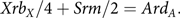
A single realization of the model was effected starting with 200 carriers and 50 with the trait. The population was followed for 1000 years, a year being 52 weeks of 7 days. Figure 1 depicts the numbers with the trait and Figure 2 the numbers of carriers over the whole period. While there are only small changes over say 3 years, there can be quite large changes over long intervals. There is low correlation between the number with the trait and the number of carriers in the short run, but moderate cross-correlation in the long run.

Fig. 1. Simulated numbers of patients at yearly intervals (S = 2,800,000, m = 12 × 10−6, s = 60 × 10−6, b X = 7/4, b A = ½, d X = 1 and d A = 2).
Fig. 2. Simulated numbers of carrier females at yearly intervals (S = 2,800,000, m = 12 × 10−6, s = 60 × 10−6, b X = 7/4, b A = ½, d X = 1 and d A = 2).
The median number of individuals with the trait over the whole interval was 51, of carriers 194, the minima 35 and 161, and the maxima 78 and 248, respectively. The changes from week to week are summarized in Table 1, showing that changes of more than one in either the number with the trait or carriers, or both, are infrequent. While it may seem absurd to consider a phenomenon over 1000 years in a rapidly changing world, we may not know accurately the current number of carriers.
Table 1. Simulated frequencies of changes in numbers of carriers and patients from week to week over 1000 years

The expected number of hemophiliacs dying each year is Ard A, so the number of years required to replace the existing ones is 1/(rd A). This is approximately 33 and serves as an estimate of average lifespan. A similar argument applying to carriers yields the estimate 67, and the ratio of lifespans d X/d A = 1/2, in this case. Obviously, the reliability of this argument depends on the factual basis of the parameters.
The expected incidence of hemophilia B in males, from equation (13), using the speculative parameters, is 1/13,276.
Discussion
Mannucci and Tuddenham (Reference Mannucci and Tuddenham2001) give summary statistics for both A and B types of hemophilia. They state that about 30% of cases arise with no family history. The equilibrium prediction from equation (10) for type B is about 16%. These authors state that the incidence of A is 1 in 5000 and of B is 1 in 30,000.
Kling et al. (Reference Kling, Ljung, Sjörin, Montandon, Green, Giannelli and Nilsson1992) state that of 45 hemophilia B patients registered at the hemophilia center in Malmö, Sweden, 24 were the sole members of their families to be affected. In 13 of the 24, ascendant relatives were available for study. Ten of these inherited the defect from mothers and three, that is roughly one-quarter, had de novo mutations. All the 10 carrier mothers had de novo mutations. Six of the 10 carrier mothers were informative as to the origin of the mutation, which were all paternal. These authors report ‘the relatively high turnover of the haemophilia-B gene pool’ (p. 144).
Ljung et al. (Reference Ljung, Petrini, Tengborn and Sjörin2001) give a succinct summary of the characteristics of hemophilia B based on Swedish data. They divide cases into ‘severe’, ‘moderate’ and ‘mild’. The range and complexity of their findings show that a model such as the one presented here presents a very simplified picture.
Mannucci and Tuddenham (Reference Mannucci and Tuddenham2001) discuss the use of plasma concentrates of coagulation factors and transmission of hepatitis virus and HIV. Medical intervention, while desirable for families, creates problems for epidemiologists.
Crew (Reference Crew1947, p. 49) contains some population genetics theory: ‘If the frequency of haemophilic males among the male population is p and the frequency of normal males is q, where (p + q) = 1, then with random mating, the frequency of haemophiliacs, carriers and normals among the female population is p 2: 2pq: q 2’. The derivation is based on the assumption that the frequency of the hemophilic gene is the same in males as females. In the notation used here this is equivalent to asserting 2A = X, which is not generally the case in the model population.
Applying equation (14) predicts HEMB gene frequency to be 6.08 × 10⁻⁵ and the heterozygote, that is carrier number, from the Hardy–Weinberg distribution evoked by Crew, in the virtual population to be 170. Figure 2 suggests that this is too low.


