


1. Introduction
Economic activity and uncertainty regarding key political, financial, and economic issues appear to be negatively related. As economic uncertainty increases, firms and consumers tend to postpone consumption and investment decisions and become more risk averse. Consequently, firms tend to reduce hiring and investment (Bloom (Reference Bloom2009), Caggiano et al. (Reference Caggiano, Castelnuovo and Groshenny2014), Kang et al. (Reference Kang, Lee and Ratti2014), Baker et al. (Reference Baker, Bloom and Davis2016), Caldara et al. (Reference Caldara, Fuentes-Albero, Gilchrist and Zakrajšek2016), Basu and Bundick (Reference Basu and Bundick2017), Bloom et al. (Reference Bloom, Floetotto, Jaimovich, Saporta-Eksten and Terry2018)), banks tend to reduce lending (Bordo et al. (Reference Bordo, Duca and Koch2016)), and financial markets tend to become more volatile (Boutchkova et al. (Reference Boutchkova, Doshi, Durnev and Molchanov2012), Pástor and Veronesi (Reference Pástor and Veronesi2013), Liu and Zhang (Reference Liu and Zhang2015)).Footnote 1 As a result, economic uncertainty can cause severe output fluctuations.Footnote 2
The global financial crisis of 2008/2009 and the COVID-19 pandemic are current examples of extraordinary high economic uncertainty. These experiences and the potentially severe negative effects of economic uncertainty on financial markets and real economic activity therefore greatly increase the demand for indicators of economic uncertainty. However, economic uncertainty is a fuzzy concept as different economic agents can have different levels of knowledge and very different views about the future. As a result, there is no single “true” measure of economic uncertainty. Rather, economic uncertainty can be measured from different angles.
Various indicators of economic uncertainty have been proposed in the literature. News-based economic policy uncertainty (EPU) indices are based on text searches in newspapers for keywords that reflect economic and political uncertainty (Baker et al. (Reference Baker, Bloom and Davis2016)).Footnote 3 Survey-based indicators of uncertainty measure the amount of disagreement about the evolution of key economic variables (Bachmann et al. (Reference Bachmann, Elstner and Sims2013)). Further measures of economic uncertainty include indicators extracted from a large set of economic time series (Jurado et al. (Reference Jurado, Ludvigson and Ng2015), Scotti (Reference Scotti2016)), distribution-based measures (Rossi and Sekhposyan (Reference Rossi and Sekhposyan2015)), and measures of stock market volatility (Datta et al. (Reference Datta, Londono, Sun, Beltran, RT Ferreira, Iacoviello, Jahan-Parvar, Li, Rodriguez and Rogers2017)). A common factor of these indicators is that they are based on complex and data-intensive methods, are often only available for a few large economies, or that they depend on well developed stock markets.
Against this background, we empirically investigate whether the volatility of sovereign credit default swap (CDS) spreads contains information about economic uncertainty. A sovereign CDS is a credit derivative that provides protection against financial losses from government defaults or sovereign debt restructuring. The CDS spread is the periodic premium that must be paid for protection, which ultimately depends on the economic conditions in a country.Footnote 4 In addition, sovereign CDS contracts are mainly traded by the world’s largest banks in the derivative business—the so-called G16 traders. The volatility of sovereign CDS spreads should, therefore, reflect uncertainty of these global banks regarding the prevailing economic conditions and prospects in a country. As a result, sovereign CDS volatility could provide another potentially complementary angle to gauge economic uncertainty. We refer to this as an outside view on economic uncertainty. Since CDS contracts are traded for almost all countries, the availability of this uncertainty indicator does not depend on country-specific data issues (e.g., availability of news- or survey-based indicators) or well-developed equity markets. Sovereign CDS volatility thus provides policymakers and researchers with an outside view on economic uncertainty that is available for almost all countries.
We examine the usefulness of sovereign CDS volatility as an indicator of economic uncertainty for three groups of economies: Euro area countries (France, Germany, Ireland, Italy, Netherlands, and Spain), major advanced economies (Canada, Great Britain, Japan, South Korea, Sweden, and USA), and emerging market economies (Brazil, Croatia, Mexico, and Russia). For that purpose, we examine the empirical relationship between CDS volatility and the news-based EPU indices of Baker et al. (Reference Baker, Bloom and Davis2016), as these indices are very popular and widely used by practitioners as a measure of economic uncertainty. As our country selection indicates, the coverage of the EPU indices is currently still limited, however.
We proceed in three steps: First, we compare the evolution of sovereign CDS volatility over time with that of EPU indices. In that regard, we also examine whether sovereign CDS volatility rises around election dates—a feature of EPU indices that has been demonstrated in the literature (Baker et al. (Reference Baker, Baksy, Bloom, Davis and Rodden2020)).
Second, we investigate whether the volatility of sovereign CDS spreads and EPU indices share directional information. We focus on directional predictions because EPU indices and CDS volatility cannot be directly compared numerically. The volatility of CDS spreads is measured in basis points, while EPU indices are dimensionless and arbitrarily normalized to an average level of 100. Thus, direct numerical comparisons of CDS volatility and EPU indices are not meaningful. We therefore examine how often we can successfully predict an upward (downward) movement in the EPU index using the upward (downward) movement in CDS volatility as a predictor. As discussed later in Section 3, CDS volatility and EPU indices capture the uncertainty of different economic agents. Nevertheless, we expect the directional movements of both indicators to coincide at least to some extent.
Third, we compare macroeconomic responses to an economic uncertainty shock when uncertainty is measured by different indicators. We provide a comparison of uncertainty shocks measured by CDS volatility to uncertainty shocks measured with the EPU index or by equity volatility. For the US, we also compare the macroeconomic consequences to uncertainty shocks measured by the financial uncertainty index of Jurado et al. (Reference Jurado, Ludvigson and Ng2015). To do so, we estimate a Bayesian (panel) vector autoregression (VAR) and identify uncertainty shocks following Bloom (Reference Bloom2009). This allows us to compute impulse response functions (IRFs) across the different country groups we consider. Specifically, we investigate the impulse responses of output and unemployment to uncertainty shocks.
Our main results can be summarized as follows: Sovereign CDS volatility seems to primarily capture economic and financial uncertainty rather than political uncertainty. The directional predictions for EPU indices based on directional changes in sovereign CDS volatility are in almost all cases better than random predictions. Hence, directional changes in sovereign CDS volatility contain some information about directional changes in the corresponding EPU country index. For most countries, the fraction of correct directional predictions is between 55% and 60%. For some countries (i.e., Great Britain, Mexico, Brazil, and South Korea) this fraction exceeds 60%. The empirical results from the panel VAR reveal that the responses of output and unemployment to shocks to sovereign CDS volatility and EPU indices are qualitatively similar in all three groups of countries. Output declines and unemployment rises after an uncertainty shock, no matter whether uncertainty is measured by CDS volatility or by an EPU index. However, our results show that responses to CDS volatility shocks exhibit a much clearer pattern than to EPU index shocks. Furthermore, the reactions to uncertainty shocks, measured by sovereign CDS volatility or equity volatility, are quite similar in shape and size. Finally, we find that the US-specific responses to shocks in sovereign CDS volatility and responses to financial uncertainty shocks are also similar.
The rest of the paper is structured as follows. In the next section, we describe the data. In Section 3, we outline the computation of sovereign CDS volatility, discuss why sovereign CDS volatility captures economic uncertainty, and explain similarities and differences with other measures of economic uncertainty. Section 4 deals with the evaluation of directional predictions for EPU indices based on CDS volatility. In Section 5, we outline the panel VAR methodology, present the results for the macroeconomic responses to uncertainty shocks, and report some additional robustness analysis. Section 6 provides conclusions.
2. Data
Our main data consist of the standard macroeconomic variables output (as measured by industrial production), unemployment, short-term interest rates, equity prices, and daily data on sovereign CDS spreads and monthly data on EPU country indices. The macroeconomic data are obtained from Eurostat, the IMF, and the OECD. The CDS spreads come from the Macrobond database.Footnote 5 The EPU indices come from the Economic Policy Uncertainty homepage maintained by Baker et al. (Reference Baker, Bloom and Davis2016).Footnote 6 We were able to collect complete data on all variables for 16 countries. We divide these countries into three groups: the Euro area (France, Germany, Ireland, Italy, Netherlands, and Spain), major advanced economies (Canada, Great Britain, Japan, South Korea, Sweden, and USA), and emerging market economies (Brazil, Croatia, Mexico, and Russia).
The sample period in our baseline analysis ranges from 2008m10 to 2019m12. We do not start earlier because the CDS market was essentially illiquid for most countries until the US investment bank Lehman Brothers went bankrupt in September 2008. CDS trading on government debt started already around the year 2000, but CDS contracts were initially traded only for Brazil, Japan, Mexico, the Philippines, and South Africa—all countries with serious economic problems at that time (Packer and Suthiphongchai (Reference Packer and Suthiphongchai2003)). Only after the Lehman collapse, CDS contracts were traded on a large scale for all countries in our sample. For the emerging market economies where the CDS market was liquid earlier, we also consider the larger sample period from 2003m1 to 2019m12 when we compute responses to economic uncertainty shocks.
2.1. Computation of CDS volatility
We calculate CDS volatility at a monthly frequency from the daily CDS spread quotes for five-year sovereign CDS contracts denoted in US dollars because this type of contract is most frequently traded in the market (Vogel et al. (Reference Vogel, Bannier and Heidorn2013)). For each country, we compute CDS volatility in three steps. First, we calculate daily CDS spread changes $\Delta s_{t} = s_{t} - s_{t-1}$
, (
$\Delta s_{t} = s_{t} - s_{t-1}$
, ( $t = 1, \ldots, T$
). We use changes because the spreads
$t = 1, \ldots, T$
). We use changes because the spreads $s_{t}$
themselves are not stationary. Only unpredictable movements in CDS spreads thus contribute to CDS volatility. Therefore, we then regress the daily CDS spread changes on their first five lags
$s_{t}$
themselves are not stationary. Only unpredictable movements in CDS spreads thus contribute to CDS volatility. Therefore, we then regress the daily CDS spread changes on their first five lags
 \begin{equation} \Delta s_{t} = \alpha _{0} + \alpha _{1}\Delta s_{t-1} + \ldots + \alpha _{4} \Delta s_{t-5} + e_{t} \end{equation}
to remove any predictable mean dynamics. The resulting residuals in equation (1) are the unpredictable movements in CDS spreads. In the final step, we compute CDS volatility at monthly frequency from the absolute values $\vert e_{i}\vert$
of the residuals in month
$\vert e_{i}\vert$
of the residuals in month $m$
as
$m$
as
 \begin{equation} \sigma _{m} = a\sqrt{\frac{\pi }{2}}\sum ^{D_{m}}_{i = 1}\frac{\vert e_{t}\vert }{D_{m}}, \end{equation}
where $D_{m}$
is the number of trading days in month
$D_{m}$
is the number of trading days in month $m$
, and
$m$
, and $a = \sqrt{252}$
is a scaling factor that converts the average daily volatility into annualized volatility.
$a = \sqrt{252}$
is a scaling factor that converts the average daily volatility into annualized volatility.
We use the absolute values of the residuals to obtain a measure of CDS volatility that is robust against extreme observations. The term $\sqrt{\pi/2}$
in equation (2) results from the fact that the expectation of the absolute value of a random variable
$\sqrt{\pi/2}$
in equation (2) results from the fact that the expectation of the absolute value of a random variable $R=\sigma \cdot u$
is
$R=\sigma \cdot u$
is $E(\vert R \vert ) = \sigma \sqrt{2/\pi }$
when
$E(\vert R \vert ) = \sigma \sqrt{2/\pi }$
when $\sigma$
is a positive constant and
$\sigma$
is a positive constant and $u$
is standard normally distributed.
$u$
is standard normally distributed.
Table A.1 and Table A.2 in Appendix A summarize the main statistical properties of the daily CDS spreads and the resulting monthly CDS volatility series. There it can be seen that Spain, Italy, Ireland, Brazil, Croatia, Mexico, and Russia—the countries with higher CDS spreads—are also the countries that display higher CDS volatility.
3. Sovereign CDS volatility and economic uncertainty
In this section, we explain why sovereign CDS volatility captures economic uncertainty, discuss differences and similarities with other measures of uncertainty, and relate it to EPU indices.
3.1. CDS volatility and economic uncertainty
As already mentioned, sovereign CDS volatility reflects the uncertainty of traders in global banks about the prevailing economic conditions and prospects in a country. We now discuss in more detail why and which facets of economic uncertainty sovereign CDS volatility might capture.
The pricing of CDS contracts provides some insights. The CDS spread $s_{t}$
is approximately equal to
$s_{t}$
is approximately equal to
 \begin{equation} s_{t} \approx lgd \cdot pd^Q_{t} = lgd \cdot pd_{t} + rp_{t} \mbox{,} \end{equation}
where $lgd$
is the loss given default and
$lgd$
is the loss given default and $pd^Q_{t}$
is the risk neutral default probability. Substituting the objective default probability
$pd^Q_{t}$
is the risk neutral default probability. Substituting the objective default probability $pd_{t}$
(which is typically smaller than
$pd_{t}$
(which is typically smaller than $pd^Q_{t}$
) for the risk neutral default probability yields the second expression, which defines the CDS spread as the sum of the objective expected loss
$pd^Q_{t}$
) for the risk neutral default probability yields the second expression, which defines the CDS spread as the sum of the objective expected loss $lgd \cdot pd_{t}$
and a risk premium
$lgd \cdot pd_{t}$
and a risk premium $rp_{t}$
. See Amato (Reference Amato2005), Berg (Reference Berg2010), Das et al. (Reference Das, Hanouna and Sarin2009) for further details.Footnote
7
A CDS is priced assuming a constant loss given default over the life of the contract.Footnote
8
Changes in the CDS spread
$rp_{t}$
. See Amato (Reference Amato2005), Berg (Reference Berg2010), Das et al. (Reference Das, Hanouna and Sarin2009) for further details.Footnote
7
A CDS is priced assuming a constant loss given default over the life of the contract.Footnote
8
Changes in the CDS spread $\Delta s_{t}$
therefore essentially reflect changes in the objective probability of default and the degree of risk aversion of investors. Consequently, the volatility of CDS spread changes
$\Delta s_{t}$
therefore essentially reflect changes in the objective probability of default and the degree of risk aversion of investors. Consequently, the volatility of CDS spread changes $\sigma _{m}$
reflects uncertainty about the evolution of the determinants of a country’s default probability and fluctuations in risk aversion.
$\sigma _{m}$
reflects uncertainty about the evolution of the determinants of a country’s default probability and fluctuations in risk aversion.
Empirical work suggests that a country’s default probability depends mainly on the government’s effectiveness in collecting taxes and using them efficiently (Jeanneret (Reference Jeanneret2018)), fiscal space (i.e., debt and deficit relative to tax revenues), inflation, trade openness, external debt (Aizenman et al. (Reference Aizenman, Hutchison and Jinjarak2013)), the size and state of the economy, and the size and health of the financial system (Dieckmann and Plank (Reference Dieckmann and Plank2012)). In addition to these country-specific variables, the literature finds that global risk factors reflecting exposure to US business cycle risk (Longstaff et al. (Reference Longstaff, Pan, Pedersen and Singleton2011)) and global risk aversion (Remolona et al. (Reference Remolona, Scatigna and Wu2008)) also help to explain CDS spreads. It seems that global risk factors tend to be more important in normal times, while country-specific variables become more important in times of crisis (Augustin (Reference Augustin2018)). As a result, sovereign CDS volatility captures uncertainty about country-specific economic conditions, especially during economic downturn, while in normal times sovereign CDS volatility may also partly reflect changes in global economic risk and risk aversion.
3.2. Sovereign CDS volatility and other uncertainty measures
We now briefly compare sovereign CDS volatility with other measures of economic uncertainty that have been proposed in the literature. As mentioned in the introduction, these measures fall into four broad groups: model-based measures using large sets of economic indicators, market-based measures, survey-based measures, and measures based on text searches.
Model-based measures of uncertainty (Jurado et al. (Reference Jurado, Ludvigson and Ng2015), Scotti (Reference Scotti2016), Ludvigson et al. (Reference Ludvigson, Ma and Ng2020)) and sovereign CDS volatility are similar in that both use forecast errors from econometric models to obtain an uncertainty measure. They differ in that the former approaches use information from many economic series and computationally intensive methods, while we use quoted CDS spreads and the computationally simple equations (1) and (2) to construct our CDS-based measure of economic uncertainty.
Market-based uncertainty measures such as realized stock market volatility are conceptually similar to sovereign CDS volatility and differ mainly in the underlying variable. Another notable difference is that stock market volatility is often computed from raw stock index returns (Poon and Granger (Reference Poon and Granger2003), Ederington and Guan (Reference Ederington and Guan2006)), whereas we first remove the predictable variation in CDS spread changes to avoid mixing the predictable variation with the unpredictable variation in computing sovereign CDS volatility.
Survey-based uncertainty measures (Bachmann et al. (Reference Bachmann, Elstner and Sims2013), Leduc and Liu (Reference Leduc and Liu2016), Altig et al. (Reference Altig, Barrero, Bloom, Davis, Meyer and Parker2022)) use disagreement of households, professional forecasters, or firms about future business, expenditures, and future economic activity. A similarity between survey-based measures and our CDS-based uncertainty measure is that both use information generated by specific economic agents. Survey methods use discrepancies of forecasts from professional forecasters, firms, and households, while sovereign CDS volatility uses fluctuations in CDS spreads to capture CDS traders uncertainty about a country’s economic health.
Text-based uncertainty measures are constructed from searches for keywords related to uncertainty in newspapers (Baker et al. (Reference Baker, Bloom and Davis2016), Husted et al. (Reference Husted, Rogers and Sun2020), Caldara et al. (Reference Caldara, Iacoviello, Molligo, Prestipino and Raffo2020)), other publications (Ahir et al. (Reference Ahir, Bloom and Furceri2022)), or the internet (Bontempi et al. (Reference Bontempi, Frigeri, Golinelli and Squadrani2021)). The monthly available EPU indices from Baker et al. (Reference Baker, Bloom and Davis2016) are the most popular, but unlike sovereign CDS volatility, the indices are only available for a limited number of countries. The World Uncertainty Index (WUI) is a relatively new measure, based on keyword searches in Economist Intelligence Unit country reports and available quarterly and monthly for about 140 countries (Ahir et al. (Reference Ahir, Bloom and Furceri2022)).
As with survey-based approaches, sovereign CDS volatility and text-based indices have in common that the information about uncertainty comes from specific agents. In the case of CDS volatility, the information comes from CDS traders, while EPU indices use information from journalists and WUI indices are based on expert opinions.
3.3. Sovereign CDS volatility, EPU and WUI indices
The news-based EPU index introduced in Baker et al. (Reference Baker, Bloom and Davis2016) is the benchmark measure of economic uncertainty in our analysis, as it is arguably the most popular measure of economic uncertainty at present. In addition, EPU indices have also been found to help explain CDS spreads (Wisniewski and Lambe (Reference Wisniewski and Lambe2015)). The WUI index is a new text-based measure of uncertainty that has recently become available for a large number of countries. We now compare sovereign CDS volatility with EPU and WUI indices.
Fig. 1 shows how sovereign CDS volatility (black, solid line), EPU (red, dashed line), and WUI (blue, solid line), averaged over all countries in the sample, evolved over time. For better comparability, the series are standardized. As can bee seen, average CDS volatility already peaked at the beginning of the sample period due to the financial crisis. In 2010 and 2012, two more spikes occurred because of the European debt crisis. From 2017 onward, average CDS volatility was relatively low. However, some of the individual volatility series remained quite high and sometimes reached levels of more than 200 basis points.
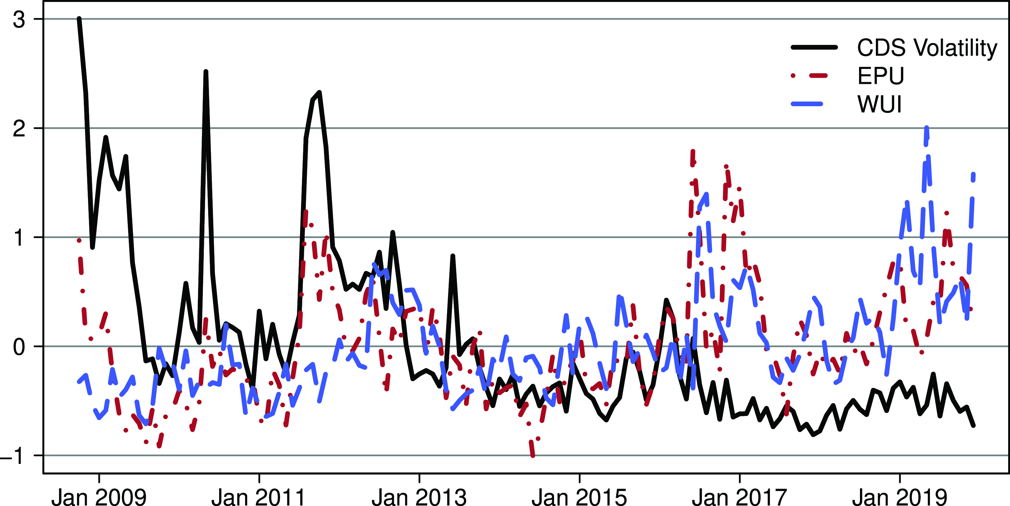
Figure 1. CDS volatility, EPU, and WUI. Notes: Bold black line denotes the cross-sectional average of CDS volatility, the red dashed-dotted line denotes the cross-sectional average of EPU, and the blue dashed line is the WUI. All series are standardized.
In comparison, average WUI and EPU are more similar and higher in the second half of the sample period. The summary statistics in Table A.3 in Appendix A show that average EPU was particularly high for Brazil, Canada, China, France, and Great Britain. In these countries, the unusually high index values occurred mainly in the last few years of the sample period. Recent political scandals provide an explanation for Brazil. The rough US trade policy is likely to be responsible for this pattern in Canada and China. Uncertainty surrounding the planned exit from the European Union explains the high EPU index values for Great Britain, and a series of ISIS terror attacks is responsible for the high index values for France. The peaks in the standardized average EPU are shown in Fig. 1.
Fig. 2 shows the evolution of the individual and average series for CDS volatility (left column), EPU (middle column), and WUI (right column) for our three country groups. The following observations stand out. Standardized CDS volatility is on average somewhat lower than standardized EPU and WUI toward the end of the sample period. The individual EPU and WUI series tend to fluctuate more than the CDS volatility series. The peaks in the average CDS volatility series are more pronounced than in the EPU and WUI series in the crisis years 2009, 2010, and 2012. In contrast, EPU and WUI are peaking around 2016–2017 when Trump was elected, the UK held the Brexit referendum, and several countries including Brazil, France, and South Korea faced political turmoils. The patterns for the CDS volatility, EPU and WUI indices thus suggest that WUI and EPU react more strongly to political uncertainty, while sovereign CDS volatility tends to react more sharply to financial uncertainty.

Figure 2. CDS volatility and EPU across country groups. Notes: Gray thin lines denote country-specific standardized CDS volatility and EPU series, while the bold black line denotes the cross-sectional average. The country groups are defined as follows: advanced economies (CA, GB, JP, KR, SE, and US), euro area economies (DE, ES, FR, IE, IT, and NL), and emerging market economies (BR, HR, MX, and RU).
3.4. Sovereign CDS volatility and elections
Ahir et al. (Reference Ahir, Bloom and Furceri2022) find that WUI indices, similar to EPU indices, increase around elections and therefore capture political uncertainty.Footnote 9 To see whether sovereign CDS volatility reacts to political uncertainty, we follow these authors and investigate whether CDS volatility changes around election dates.
We collect data on election dates for our 16 countries over the time period from 2008M10 to 2019M12 from https://www.electionguide.org/. The data cover dates on national elections (parliamentary, presidency, and regional) as well as referendums. Our sample includes dates for 91 elections. As in Ahir et al. (Reference Ahir, Bloom and Furceri2022), we estimate a panel model including two lags and leads of election period dummies:
 \begin{equation} \sigma _{it} = \alpha _i + \beta _t + \sum _{j=-2}^{2} \delta _j D_{it-j} + \eta _{it}, \quad \eta _{it} \sim \mathcal{N}(0,\sigma _{\eta }^2), \end{equation}
where $\sigma _{it}$
denotes CDS volatility in country
$\sigma _{it}$
denotes CDS volatility in country $i=1,\ldots,N$
and time period
$i=1,\ldots,N$
and time period $t=1,\ldots,T$
. The coefficients
$t=1,\ldots,T$
. The coefficients $\alpha _i$
and
$\alpha _i$
and $\beta _t$
denote country and time fixed effects, and
$\beta _t$
denote country and time fixed effects, and $D_{it}$
is a dummy variable that takes a value of
$D_{it}$
is a dummy variable that takes a value of $1$
if in country
$1$
if in country $i$
and time period
$i$
and time period $t$
an election has occurred, and zero otherwise. We thus estimate a total of five models and include only one dummy variable per model (contemporaneous, two lags, and two leads). For instance, in the model examining the contemporaneous effects (
$t$
an election has occurred, and zero otherwise. We thus estimate a total of five models and include only one dummy variable per model (contemporaneous, two lags, and two leads). For instance, in the model examining the contemporaneous effects ( $j=0$
),
$j=0$
), $\delta _{-2}=\delta _{-1}=\delta _{1}=\delta _{2}=0$
. The error term,
$\delta _{-2}=\delta _{-1}=\delta _{1}=\delta _{2}=0$
. The error term, $\eta _{it}$
is assumed to be normally distributed with zero mean and variance
$\eta _{it}$
is assumed to be normally distributed with zero mean and variance $\sigma _\eta ^2$
.
$\sigma _\eta ^2$
.
Table 1 presents the results. The results suggest that CDS volatility and election periods are not related.Footnote 10 CDS volatility is slightly lower before elections and increase somewhat after elections. However, these effects are not statistically significant at conventional confidence levels. The results are therefore consistent with our observation in Section 3.3, namely that CDS volatility primarily captures financial and economic uncertainty is not driven by political uncertainty to the same extent as WUI and EPU indices.
Table 1. CDS volatility and elections

Notes: This table contains estimates of panel regressions. Number in parentheses denote standard errors. $^{*}$
,
$^{*}$
, $^{**}$
, and
$^{**}$
, and $^{***}$
mark statistical significance at 10%, 5%, and 1%, respectively.
$^{***}$
mark statistical significance at 10%, 5%, and 1%, respectively.
4. Common directional information in sovereign CDS volatility and EPU indices
In this section, we examine whether sovereign CDS volatility and EPU indices share directional information about economic uncertainty. More precisely, we ask whether the directional change of sovereign CDS volatility in month $m$
predicts (i.e., nowcasts) the directional change of the corresponding EPU country index in month
$m$
predicts (i.e., nowcasts) the directional change of the corresponding EPU country index in month $m$
. We use directional forecast evaluation methods to answer this question.Footnote
11
We evaluate the directional predictions by computing performance statistics and regression-based statistical tests.
$m$
. We use directional forecast evaluation methods to answer this question.Footnote
11
We evaluate the directional predictions by computing performance statistics and regression-based statistical tests.
4.1. Methods for evaluating directional predictions
To assess the predictive ability of sovereign CDS volatility, we compute four performance statistics based on the contingency matrix in Table 2. In this matrix, the indicator variable $x_{t}$
takes on the value of one when the volatility of CDS spreads has increased from time
$x_{t}$
takes on the value of one when the volatility of CDS spreads has increased from time $t-1$
to time
$t-1$
to time $t$
and is zero otherwise. Analogously, the indicator variable
$t$
and is zero otherwise. Analogously, the indicator variable $y_{t}$
takes on a value of one when the EPU index has increased from
$y_{t}$
takes on a value of one when the EPU index has increased from $t-1$
to
$t-1$
to $t$
and is zero otherwise. The entries
$t$
and is zero otherwise. The entries $N_{uu}$
and
$N_{uu}$
and $N_{dd}$
denote the number of correct up and down predictions, and the entries
$N_{dd}$
denote the number of correct up and down predictions, and the entries $N_{ud}$
and
$N_{ud}$
and $N_{du}$
denote the number of incorrect up predictions and incorrect down predictions.
$N_{du}$
denote the number of incorrect up predictions and incorrect down predictions.
The first statistic that we compute summarizes the overall accuracy of the directional predictions. Accuracy is defined as
 \begin{equation} AC = \frac{N_{uu} + N_{dd}}{N_{uu} + N_{du} + N_{ud} + N_{dd}}. \end{equation}
The value of the $AC$
statistic is between zero and one and shows the proportion of correct predictions. The statistic is intuitive but can be misleading if upward or downward movements are rare.
$AC$
statistic is between zero and one and shows the proportion of correct predictions. The statistic is intuitive but can be misleading if upward or downward movements are rare.
The next statistic, the so called “hit rate,” is defined as
 \begin{equation} HI = \frac{N_{uu}}{N_{uu} + N_{du}}, \end{equation}
and also has a value between zero and one. The hit rate $HI$
is the proportion of correct up predictions and can be recognized as a sample estimate of the conditional probability that CDS volatility will increase when EPU rises. The statistic is sensitive to upward movements but ignores false upward predictions.
$HI$
is the proportion of correct up predictions and can be recognized as a sample estimate of the conditional probability that CDS volatility will increase when EPU rises. The statistic is sensitive to upward movements but ignores false upward predictions.
The “false alarm rate” is defined as
 \begin{equation} F = \frac{N_{ud}}{N_{ud} + N_{dd}}, \end{equation}
looks at the the proportion of incorrect upward predictions. The statistic provides an estimate of the conditional probability of an incorrect upward prediction when the EPU index actually goes down. The related quantity $1 - F$
is an estimate of the conditional probability that CDS volatility provides a correct downward prediction when the EPU actually did go down.
$1 - F$
is an estimate of the conditional probability that CDS volatility provides a correct downward prediction when the EPU actually did go down.
Table 2. Contingency matrix for directional predictions

Notes: $N_{uu}$
denote the number of correct up predictions,
$N_{uu}$
denote the number of correct up predictions, $N_{dd}$
the number of correct down predictions,
$N_{dd}$
the number of correct down predictions, $N_{ud}$
the number of incorrect up predictions, and
$N_{ud}$
the number of incorrect up predictions, and $N_{du}$
the number of incorrect down predictions.
$N_{du}$
the number of incorrect down predictions.
The difference between the hit rate and the false alarm rate is known as the Kuiper score:
 \begin{equation} KS = 100\cdot (HI - F). \end{equation}
The $KS$
statistic has a range of [-100, 100] and indicates how well CDS volatility discriminates between up and down movements in the EPU index over time. The
$KS$
statistic has a range of [-100, 100] and indicates how well CDS volatility discriminates between up and down movements in the EPU index over time. The $KS$
statistic is around zero if the directional predictions are essentially random. A positive
$KS$
statistic is around zero if the directional predictions are essentially random. A positive $KS$
statistic indicates that CDS volatility helps to predict the directional movements of an EPU index.
$KS$
statistic indicates that CDS volatility helps to predict the directional movements of an EPU index.
The statistics just described examine the ability of movements in CDS volatility to correctly capture movements in EPU indices, but they are not formal statistical tests. We therefore also perform two regression-based statistical tests suggested in Blaskowitz and Herwartz (Reference Blaskowitz and Herwartz2014). Both tests use the indicator variables $x_{t}$
and
$x_{t}$
and $y_{t}$
for up and down movements in CDS volatility and the corresponding EPU index. In both tests, the null hypotheses of zero covariance between
$y_{t}$
for up and down movements in CDS volatility and the corresponding EPU index. In both tests, the null hypotheses of zero covariance between $x_{t}$
and
$x_{t}$
and $y_{t}$
implies that the directional predictions based on CDS volatility are purely random.
$y_{t}$
implies that the directional predictions based on CDS volatility are purely random.
In the first test, we run the linear regression
 \begin{equation} y_{t} = \alpha + \beta x_{t} + u_{t} \end{equation}
and test for $\beta = 0$
. This test assumes that the error
$\beta = 0$
. This test assumes that the error $u_{t}$
in (9) has zero mean, a constant variance, and is serially uncorrelated (i.e.,
$u_{t}$
in (9) has zero mean, a constant variance, and is serially uncorrelated (i.e., $E(u^2_{t}|x_{t}, x_{t-1},\ldots ) = \sigma ^2 \gt 0$
and
$E(u^2_{t}|x_{t}, x_{t-1},\ldots ) = \sigma ^2 \gt 0$
and $E(u_{t}u_{s}|x_{t}, x_{t-1},\ldots ) = 0$
for all
$E(u_{t}u_{s}|x_{t}, x_{t-1},\ldots ) = 0$
for all $t \neq s$
). Under these assumptions, the hypotheses
$t \neq s$
). Under these assumptions, the hypotheses $\beta = 0$
can be tested with a standard t-test.
$\beta = 0$
can be tested with a standard t-test.
In the second test, these assumptions can be relaxed by running an augmented regression of the type
 \begin{equation} y_{t} = \alpha + \beta x_{t} + \sum ^m_{j=1}\gamma _{j}x_{t-j} + \sum ^n_{j=1}\delta _{j}y_{t-j} + u_{t} \end{equation}
that corrects for the effects of lagged dependent and explanatory variables. The hypothesis to be tested is again $\beta = 0$
. To account for any remaining autocorrelation in the residuals, we compute the t-test statistic with robust Newey–West standard errors (Newey and West (Reference Whitney and West1987)).
$\beta = 0$
. To account for any remaining autocorrelation in the residuals, we compute the t-test statistic with robust Newey–West standard errors (Newey and West (Reference Whitney and West1987)).
4.2. Results of directional predictions
In this section, we present the empirical findings about the ability of monthly sovereign CDS volatility to predict the directional change of the corresponding EPU country index in the same month. We begin with the performance statistics in Table 3.
Table 3. Pearson and Spearman correlation between original EPU and CDS volatility series

The upper left plot in Fig. 3 shows the results for the hit rate, defined as the proportion of correct upward predictions. As can be seen, twelve out of sixteen hit rates exceed 50%. The hit rates reach about 57.5% for France, Brazil, Italy, the US, Great Britain, South Korea, and Spain. The hit rates for Canada, Croatia, and Mexico are around 55%. However, CDS volatility does not always help predict upward movements in EPU. The hit rates for the Netherlands, Ireland, Russia, and Japan are below 50%.

Figure 3. Directional forecast statistics.
The upper right diagram shows that the directional predictions from CDS volatility do not produce excessively high false alarm rates. The proportion of incorrect upward predictions is for almost all countries well below 50%. With values close to 32%, the false alarm rates are particularly low for Brazil, South Korea, and Mexico. Most other false alarm rates are between 35% and 45%. An exception is Ireland, where the false alarm rate reaches 50%.
Accuracy—the proportion of correct predictions—is for fourteen out of sixteen countries above 50%. For eleven countries, accuracy is 56% or higher. Due to the high hit rates and low false alarm rates, the accuracy of the directional predictions for Brazil and South Korea is particularly high and exceeds 62%. Exceptions are the Netherlands and again Ireland where accuracy is only about 48%. The lower right diagram in Fig. 3 shows the country-specific Kuiper scores that indicate how well changes in CDS volatility predict the directional changes in EPU over time. The Kuiper score is positive for fourteen out of sixteen countries. Thus over time, changes in CDS volatility produce more correct than incorrect directional forecasts of the corresponding EPU index movements. The familiar exceptions are again Ireland and the Netherlands.
Let us now turn to the results of the regression-based tests of the predictive ability of changes in CDS volatility. Recall that in the test regressions, the $\beta$
coefficient measures the correlation between the directional movements in the EPU index and the directional movements in CDS volatility. Fig. 4 displays the estimated
$\beta$
coefficient measures the correlation between the directional movements in the EPU index and the directional movements in CDS volatility. Fig. 4 displays the estimated $\beta$
coefficient in the static and the dynamic test regressions together with 90% confidence intervals. As can be seen, the results from the static regression, shown in the left plot, and the results from the dynamic regression in the right plot are very similar. In particular, with the exception of Ireland and the Netherlands, the estimated
$\beta$
coefficient in the static and the dynamic test regressions together with 90% confidence intervals. As can be seen, the results from the static regression, shown in the left plot, and the results from the dynamic regression in the right plot are very similar. In particular, with the exception of Ireland and the Netherlands, the estimated $\beta$
coefficients are always positive in both test regressions. Most of the
$\beta$
coefficients are always positive in both test regressions. Most of the $\beta$
coefficients are between 0.1 and 0.3. The 90% confidence intervals imply that many
$\beta$
coefficients are between 0.1 and 0.3. The 90% confidence intervals imply that many $\beta$
coefficients are also statistically significant at the 10% significance level.
$\beta$
coefficients are also statistically significant at the 10% significance level.

Figure 4. Regression tests of directional forecast accuracy.
For comparison, we also show the Pearson and Spearman correlation between the original EPU and CDS volatility series in Table 3.Footnote
12
As can be seen, the correlations of the original series and the $\beta$
coefficients for the directional forecasts do not necessarily provide similar information. The correlations are more often negative and more heterogeneous than the
$\beta$
coefficients for the directional forecasts do not necessarily provide similar information. The correlations are more often negative and more heterogeneous than the $\beta$
coefficients. In contrast, the results for the
$\beta$
coefficients. In contrast, the results for the $\beta$
coefficients are much more consistent. Just two out of sixteen
$\beta$
coefficients are much more consistent. Just two out of sixteen $\beta$
’s are slightly negative. The other
$\beta$
’s are slightly negative. The other $\beta$
coefficients are all positive and often statistically significant.
$\beta$
coefficients are all positive and often statistically significant.
Taken together, the $\beta$
’s from the regression tests and the descriptive statistics for the directional forecasts tell the same story, namely that in most cases sovereign CDS volatility does contain some information about directional movements in EPU indices. Nevertheless, we observe some heterogeneity in the information content across countries, and we find that for Ireland and the Netherlands CDS volatility does not perform well in predicting movements in the news-based country EPU indices.Footnote
13
$\beta$
’s from the regression tests and the descriptive statistics for the directional forecasts tell the same story, namely that in most cases sovereign CDS volatility does contain some information about directional movements in EPU indices. Nevertheless, we observe some heterogeneity in the information content across countries, and we find that for Ireland and the Netherlands CDS volatility does not perform well in predicting movements in the news-based country EPU indices.Footnote
13
5. Macroeconomic responses to uncertainty shocks
Now, we turn to the impulse response analysis. We use a Bayesian panel VAR approach to compare the macroeconomic effects of shocks to economic uncertainty measured either by sovereign CDS volatility, the EPU index, or equity volatility.
5.1. Econometric model
The use of a panel VAR can be motivated from various angles. First, the sample length of the time series is rather short, so pooling information across countries is advantageous. Second, to also account for a degree of cross-country heterogeneity, we estimate the panel for the respective country groups separately. Last, we are interested in the average (within a country group) responses of macroeconomic quantities to economic uncertainty shocks. This renders a Bayesian panel VAR without cross-sectional heterogeneity and no static or dynamic interdependence attractive (Canova and Ciccarelli (Reference Canova and Ciccarelli2009, Reference Canova and Ciccarelli2013)).
We assume that an $M \times 1$
-dimensional multivariate time-series process
$M \times 1$
-dimensional multivariate time-series process $\{\boldsymbol{y}_{it}\}_{t=1}^T$
of each country
$\{\boldsymbol{y}_{it}\}_{t=1}^T$
of each country $i=1,\ldots,N$
follows
$i=1,\ldots,N$
follows
 \begin{equation} \boldsymbol{y}_{it} = \boldsymbol{c}_i + \sum _{j=1}^p \boldsymbol{A}_{j} \boldsymbol{y}_{it-j} + \boldsymbol{\varepsilon }_{it}, \qquad \boldsymbol{\varepsilon }_{it} \sim \mathcal{N}_M(\textbf{0},\boldsymbol{\Sigma}), \end{equation}
where the $M \times 1$
vector
$M \times 1$
vector $\boldsymbol{c}_i$
is a country-specific fixed effect, while the
$\boldsymbol{c}_i$
is a country-specific fixed effect, while the $M \times M$
coefficient matrix
$M \times M$
coefficient matrix $\boldsymbol{A}_{j}$
is fixed across countries (no dynamic cross-sectional heterogeneity). The reduced-form error term
$\boldsymbol{A}_{j}$
is fixed across countries (no dynamic cross-sectional heterogeneity). The reduced-form error term $\boldsymbol{\varepsilon }_{it}$
follows a multivariate Gaussian distribution with zero mean and covariance matrix
$\boldsymbol{\varepsilon }_{it}$
follows a multivariate Gaussian distribution with zero mean and covariance matrix $\boldsymbol{\Sigma}$
, which is also fixed across countries (no static cross-sectional heterogeneity). Cross-sectional heterogeneity is captured by the three country groups: advanced economies, Euro area economies, and emerging market economies. Further note that this structure neither allows for static nor for dynamic interdependence across countries (i.e.,
$\boldsymbol{\Sigma}$
, which is also fixed across countries (no static cross-sectional heterogeneity). Cross-sectional heterogeneity is captured by the three country groups: advanced economies, Euro area economies, and emerging market economies. Further note that this structure neither allows for static nor for dynamic interdependence across countries (i.e., $Var(\boldsymbol{y}_{it},\boldsymbol{y}_{jt})=0$
and
$Var(\boldsymbol{y}_{it},\boldsymbol{y}_{jt})=0$
and $Var(\boldsymbol{y}_{it},\boldsymbol{y}_{jt-1})=0$ $\forall i\neq j$
). In our application, this assumption is appropriate because we are not interested in measuring spillovers between countries. Instead, we want to empirically compare the transmission of economic uncertainty shocks measured with different measures of economic uncertainty across the three different groups of countries.
$\forall i\neq j$
). In our application, this assumption is appropriate because we are not interested in measuring spillovers between countries. Instead, we want to empirically compare the transmission of economic uncertainty shocks measured with different measures of economic uncertainty across the three different groups of countries.
We estimate the model with Bayesian methods. The proposed model is similar to a standard linear VAR except for the country-fixed effects. We implement the widely used Minnesota prior (Doan et al. (Reference Doan, Litterman and Sims1984), Litterman (Reference Litterman1986)). In this framework, we assume a Gaussian prior distribution on the coefficients and an inverse-Wishart prior distribution on the covariance matrix. The Minnesota prior specifies the prior belief that macroeconomic time series follow a unit root. Furthermore, it imposes the belief that higher-order lags are less important and thus closer linked to a value of zero. Practically, this means that the variance is smaller for coefficients on further lags. Finally, we impose that little is known about exogenous variables (i.e., fixed effects), so that the variance on these terms may be large. We follow standard practices as outlined in Kilian and Lütkepohl (Reference Kilian and Lütkepohl2017). We draw 10,000 posterior draws from the full posterior distribution in the Markov Chain Monte Carlo sampler and discard the first 5000 draws as burn-ins.
5.2. Data and identification
The panel VAR model contains the following six variables: the respective uncertainty indicator $x_{it}$
under consideration, the leading stock index of a country
$x_{it}$
under consideration, the leading stock index of a country $eq_{it}$
, the short-term interest rate
$eq_{it}$
, the short-term interest rate $i_{it}$
, the price level
$i_{it}$
, the price level $p_{it}$
, the unemployment rate
$p_{it}$
, the unemployment rate $u_{it}$
, and industrial production
$u_{it}$
, and industrial production $ip_{it}$
. All variables except the unemployment rate and interest rates enter in log-levels and we use the lag-length specification recommended by the Bayesian information criterion (BIC). In particular, we check the BIC up to twelve lags in each model.Footnote
14
It points to a low number of lags (either one or two lags), and thus we consistently use
$ip_{it}$
. All variables except the unemployment rate and interest rates enter in log-levels and we use the lag-length specification recommended by the Bayesian information criterion (BIC). In particular, we check the BIC up to twelve lags in each model.Footnote
14
It points to a low number of lags (either one or two lags), and thus we consistently use $p=2$
lags for all estimated models.Footnote
15
In the baseline VAR, the sample period ranges from October 2008 to December 2019. As already mentioned, for the emerging market economies in our sample, the CDS market was already liquid before the global financial crisis. For these countries, we therefore extend the sample back to January 2003 and provide results for both sample periods. This results in four country groups, which we label as follows: advanced economies, Euro area economies, emerging market economies (short sample), and emerging market economies (long sample).
$p=2$
lags for all estimated models.Footnote
15
In the baseline VAR, the sample period ranges from October 2008 to December 2019. As already mentioned, for the emerging market economies in our sample, the CDS market was already liquid before the global financial crisis. For these countries, we therefore extend the sample back to January 2003 and provide results for both sample periods. This results in four country groups, which we label as follows: advanced economies, Euro area economies, emerging market economies (short sample), and emerging market economies (long sample).
To identify the macroeconomic impact of an uncertainty shock, we rely on a standard Cholesky decomposition where the variables appear in the following ordering: $\boldsymbol{y}_{it}=\{x_{it},eq_{it},i_{it},p_{it},u_{it},ip_{it}\}$
. Thus, as in Baker et al. (Reference Baker, Bloom and Davis2016), the economic uncertainty indicator is the first variable in the system. Since uncertainty measures and stock market indices are both fast moving variables, an alternative ordering would be to put the stock index first.Footnote
16
Results with this alternative ordering are available upon request but leave our main findings unchanged.
$\boldsymbol{y}_{it}=\{x_{it},eq_{it},i_{it},p_{it},u_{it},ip_{it}\}$
. Thus, as in Baker et al. (Reference Baker, Bloom and Davis2016), the economic uncertainty indicator is the first variable in the system. Since uncertainty measures and stock market indices are both fast moving variables, an alternative ordering would be to put the stock index first.Footnote
16
Results with this alternative ordering are available upon request but leave our main findings unchanged.
5.3. Results of the impulse response analysis
This section presents the results of the impulse response analysis. For comparability, we normalize the responses to both shocks to yield a 10% decrease in the stock index. In the following, we present the impulse responses for output and unemployment to uncertainty shocks as measured by sovereign CDS volatility and the EPU country indices, respectively. We compute impulse responses for a horizon of two years (i.e., 24 months). The responses for all variables in the panel VAR can be found in Appendix B.
Figs. 5 and 6 present the impulse responses of output and unemployment to both types of uncertainty shocks. Both plots offer in four panels (one for each country group) a direct comparison between the impulse response of the model featuring uncertainty shocks measured by CDS volatility and EPU. For both indicators, we observe a decrease of economic activity after an uncertainty shock. This is consistent with findings for the US (Bloom (Reference Bloom2009), Fernández-Villaverde et al. (Reference Fernàndez-Villaverde, Guerrón-Quintana, Kuester and Rubio-Ramírez2015), Baker et al. (Reference Baker, Bloom and Davis2016), Basu and Bundick (Reference Basu and Bundick2017)).

Figure 5. Impulse responses of output to uncertainty shocks (comparison to EPU). Notes: Responses to an uncertainty shock scaled to a 10% decrease in equity prices. The reaction of output is in percent. Black solid lines denote the median effect along with 68% (dark gray), 80% (gray), and 90% (light gray) credible intervals.

Figure 6. Impulse responses of unemployment to uncertainty shocks (comparison to EPU). Notes: Responses to an uncertainty shock scaled to a 10% decrease in equity prices. The reaction of unemployment is in percent. Black solid lines denote the median effect along with 68% (dark gray), 80% (gray), and 90% (light gray) credible intervals.
The reduction of economic activity could be triggered by either the real options or the risk aversion channel. The real options channel is associated with a wait-and-see attitude of households and firms in response to heightened uncertainty, which results in a delay of consumption and investment. Following the risk aversion channel, risk-averse (domestic and international) investors demand a higher risk premium in the face of higher uncertainty, which raises the cost of finance. Furthermore, higher uncertainty leads to an expansion of left-tail events, thereby increasing the probability of default. This leads to a higher default premium. Higher economic uncertainty is thus strongly linked to increasing borrowing costs, which leads to a dampening of macro aggregates (Christiano et al. (Reference Christiano, Motto and Rostagno2014)).
The medium term response to output is clearly negative for CDS volatility across the country groups. For EPU, we observe negative effects for the emerging market sample but less clear-cut effects for advanced economies or the Euro area economies. The shocks are economically and statistically significant and sizable. The effect sizes range from a 6% (Euro area) to a 16% (emerging markets) output contraction for uncertainty shocks measured by CDS volatility. Our results are also in line with the more recent literature on the macroeconomic effects of uncertainty (Bachmann et al. (Reference Bachmann, Elstner and Sims2013), Jurado et al. (Reference Jurado, Ludvigson and Ng2015)), which finds no evidence for any overshooting effects in output. The same pattern holds also when inspecting the impulse responses of unemployment. While CDS volatility leads to a surge in unemployment, we see only significant effects for EPU in the emerging market samples. CDS volatility shocks lead to a significant rise in unemployment throughout all regions, with peak effects ranging from 5% (advanced economies) to 15% (emerging markets).
Overall, our results point to similar effects when comparing these uncertainty shocks. Nevertheless, the EPU results are less precisely estimated and do not lead to economic contractions in two out of three country groups. We argue that these differences arise because both uncertainty measures capture different information. Sovereign CDS volatility is market-based and reflects how global banks view the prevailing economic conditions in a country. EPU, however, is news-based and therefore captures not only financial uncertainty but also other facets of uncertainty. In particular, news-based uncertainty measures may be more noisy as they also capture uncertainty about political processes and economic policy that are not inherently harmful to economic outcomes.
5.4. Comparisons with further measures of economic uncertainty
As already mentioned, the literature on economic uncertainty has proposed several other uncertainty measures. Therefore, we cross-check our results with further alternatives.Footnote 17 More specifically, we use the volatility of stock index returns as an alternative measure of economic uncertainty (see also Datta et al. (Reference Datta, Londono, Sun, Beltran, RT Ferreira, Iacoviello, Jahan-Parvar, Li, Rodriguez and Rogers2017)). Stock market/equity volatility is a widely used measure of uncertainty that can be computed for all countries in the sample. For each country, we compute monthly stock market volatility from the daily returns on the leading stock index of the country.Footnote 18
Furthermore, we compare our proposed measure of uncertainty, the sovereign CDS volatility, with the financial uncertainty index introduced by Jurado et al. (Reference Jurado, Ludvigson and Ng2015) and the world uncertainty index proposed by Ahir et al. (Reference Ahir, Bloom and Furceri2022). The financial uncertainty index, which is only available for the USA, exploits a data-rich environment to generate the conditional volatility of an unforecastable disturbance to measure (financial) uncertainty.Footnote 19 Specifically, we utilize the volatility of the one-step ahead forecast error of the financial uncertainty index. Our comparison thus serves as an ideal robustness check as to whether CDS volatility captures similar information as a measure based on a high-dimensional dataset from the US real and financial economy. The WUI, on the other hand, is a new text-based measure of uncertainty and exploits the Economist Intelligence Unit country reports.Footnote 20 To ensure comparability, the model specification and the ordering of the variables in the VAR are the same as in the previous VAR models.
We begin by discussing the results of comparing sovereign CDS volatility with equity volatility as an alternative measure of economic uncertainty. The four panels in Figs. 7 and8 show the impulse responses of output and unemployment to both types of uncertainty shocks. As before, we have normalized the shock to a 10% decrease in equity prices. The responses of all variables in the panel VAR can be found in Appendix B. Overall, results show a strong similarity between sovereign CDS volatility and stock market volatility. In all country groups, output contracts and unemployment rises. The responses are economically and statistically significant. In the model with equity volatility, the effect sizes range from a decline of 4% (Euro area) to 15% (emerging markets) and are thus comparable to the results for CDS volatility. In some instances, CDS volatility even points to more detrimental effects than stock market volatility.

Figure 7. Impulse responses of output to uncertainty shocks (comparison to equity volatility). Notes: Responses to an uncertainty shock scaled to a 10% decrease in equity prices. The reaction of output is in percent. Black solid lines denote the median effect along with 68% (dark gray), 80% (gray), and 90% (light gray) credible intervals.

Figure 8. Impulse responses of unemployment to uncertainty shocks (comparison to equity volatility). Notes: Responses to an uncertainty shock scaled to a 10% decrease in equity prices. The reaction of unemployment is in percent. Black solid lines denote the median effect along with 68% (dark gray), 80% (gray), and 90% (light gray) credible intervals.
In our comparison of sovereign CDS volatility with the financial uncertainty index for the US, we estimate a single-country Bayesian VAR.Footnote 21 We also use the same recursive identification scheme as before to compute the impulse responses. The magnitude of the shocks is again normalized to a 10% decline in equity prices on impact.
We present the impulses responses of output and unemployment in Fig. 9 and the full set of impulse responses in Appendix B. As can be seen, the responses to both shocks are again qualitatively similar. In line with the literature, US economic activity strongly contracts. A few remarks are in order here. First, the peak effects are even stronger for the US than in a number of other countries. Second, the uncertainty shocks measured by the financial uncertainty indicator seem to trigger slightly weaker responses. Third, the correlation between the indicators is quite high ( $\rho =0.52$
), although they are rather differently constructed. Overall, sovereign CDS volatility and the financial uncertainty index seem to contain similar information about economic uncertainty in the USA.
$\rho =0.52$
), although they are rather differently constructed. Overall, sovereign CDS volatility and the financial uncertainty index seem to contain similar information about economic uncertainty in the USA.

Figure 9. Impulse responses to an uncertainty shock (comparison with financial uncertainty). Notes: Responses to an uncertainty shock scaled to a 10% decrease in equity prices. The reaction of output and unemployment is in percent. Black solid lines denote the median effect along with 68% (dark gray), 80% (gray), and 90% (light gray) credible intervals.
For completeness, Fig. 10 provides a comparison of sovereign CDS volatility with the WUI for the US. While the output response to a shock in the WUI is similar to the response to a shock in sovereign CDS volatility, the effects are not very precisely estimated. Unemployment responses peak at the beginning and then revert slowly. However, the effects are again not precisely estimated. Moreover, the response to a shock to sovereign CDS volatility indicates more back-loaded effects on unemployment. These rather different results suggest that sovereign CDS volatility captures other dimensions of uncertainty than the WUI that are not directly related to political events. Hence, sovereign CDS volatility is a market-based and outside view on uncertainty that appears to be more related to financial uncertainty. This agrees well with our results on election dates, where we find no association of election dates with CDS volatility.

Figure 10. Impulse responses to an uncertainty shock (comparison with world uncertainty index). Notes: Responses to an uncertainty shock scaled to a one standard deviation shock in the uncertainty indicator. The reaction of output and unemployment is in percent. Black solid lines denote the median effect along with 68% (dark gray), 80% (gray), and 90% (light gray) credible intervals.
5.5. Robustness
To check whether the results are sensitive to the number of lags in the panel VAR, we reestimate the model with different lag lengths. Figs. B.7–
B.10 show the IRFs to an uncertainty shock measured by CDS volatility, the EPU index, or equity volatility when using $p=4$
lags. The results are very similar. In particular, the responses of unemployment and output are insensitive to the number of lags in the VAR.
$p=4$
lags. The results are very similar. In particular, the responses of unemployment and output are insensitive to the number of lags in the VAR.
We also test for subsample stability by starting the sample only after the great financial crisis in 2010M1. Figs. B.11– B.13 in the appendix show the results. In the shorter sample, the responses of output and unemployment are not as pronounced as before. This is to be expected, as the last financial crisis was a major event and therefore influential on the results. Nevertheless, the results obtained with the shorter sample also suggest that uncertainty shocks reduce economic activity.
6. Conclusions
The world’s largest financial institutions are the biggest traders of sovereign CDS contracts, and sovereign CDS spreads depend on a country’s solvency. Based on these two observations, we argue that the volatility of sovereign CDS spreads provides information about country-specific economic uncertainty from the viewpoint of global financial institutions.
We compared sovereign CDS volatility with other measures of economic uncertainty using a panel of 16 countries, which we divided into major advanced economies, Euro area countries, and emerging market economies. We found that sovereign CDS volatility shares directional information with EPU country indices—a benchmark measure of economic uncertainty. We also found that the mean impulse responses of output and unemployment after an unexpected uncertainty shock are similar for all three groups of countries, regardless of whether economic uncertainty is measured by sovereign CDS volatility, an EPU index, stock market volatility, or, as in case of the USA, the financial uncertainty index of Jurado et al. (Reference Jurado, Ludvigson and Ng2015). The similarity in impulse responses, coupled with the finding that sovereign CDS volatility does not increase around election dates, suggests that sovereign CDS volatility primarily reflects financial and economic uncertainty rather than political uncertainty.
As noted earlier, there is no single true measure of economic uncertainty, and we want to emphasize that we are not claiming that sovereign CDS volatility is a better indicator of economic uncertainty than others. Nevertheless, we argue that sovereign CDS volatility is a useful indicator of economic uncertainty for at least two reasons. First, sovereign CDS volatility is easy to compute, and CDS spreads are readily available for almost all countries. Second, and more importantly, by providing information about economic uncertainty from the perspective of the world’s largest financial institutions, sovereign CDS volatility offers policymakers and researchers a valuable outside view on economic uncertainty.
Acknowledgments
The views expressed in this paper do not necessarily reflect those of the Oesterreichische Nationalbank or the Eurosystem. The authors want to thank Pia Heckl, participants of the Annual Meeting of the Austrian Economic Association as well as the editor, William Barnett, the handling associate editor, and four anonymous referees for helpful comments and suggestions.
A. Summary Statistics
Table A.1. Summary statistics of daily CDS spreads

Table A.2. Summary statistics of annualized monthly CDS volatility

Table A.3. Summary statistics of monthly EPU indices

B. Additional Results

Figure B.1. Impulse responses to uncertainty shocks in advanced economies. Notes: Responses to an uncertainty shock scaled to a 10% decrease in equity prices. Black solid lines denote the median effect along with 68% (dark gray), 80% (gray), and 90% (light gray) credible intervals.

Figure B.2. Impulse responses to uncertainty shocks in euro area economies. Notes: Responses to an uncertainty shock scaled to a 10% decrease in equity prices. Black solid lines denote the median effect along with 68% (dark gray), 80% (gray), and 90% (light gray) credible intervals.

Figure B.3. Impulse responses to uncertainty shocks in emerging market economies (short sample). Notes: Responses to an uncertainty shock scaled to a 10% decrease in equity prices. Black solid lines denote the median effect along with 68% (dark gray), 80% (gray), and 90% (light gray) credible intervals.

Figure B.4. Impulse responses to uncertainty shocks in emerging market economies (long sample). Notes: Responses to an uncertainty shock scaled to a 10% decrease in equity prices. Black solid lines denote the median effect along with 68% (dark gray), 80% (gray), and 90% (light gray) credible intervals.

Figure B.5. Comparison with financial uncertainty shocks. Notes: Responses to an uncertainty shock scaled to a 10% decrease in equity prices. Black solid lines denote the median effect along with 68% (dark gray), 80% (gray), and 90% (light gray) credible intervals.

Figure B.6. Comparison with world uncertainty index shocks. Notes: Responses to an uncertainty shock scaled to a one standard deviation shock. Black solid lines denote the median effect along with 68% (dark gray), 80% (gray), and 90% (light gray) credible intervals.

Figure B.7. Impulse responses to uncertainty shocks in advanced economies ( $p=4$
). Notes: Robustness exercise with
$p=4$
). Notes: Robustness exercise with $p=4$
. Responses to an uncertainty shock scaled to a 10% decrease in equity prices. Black solid lines denote the median effect along with 68% (dark gray), 80% (gray), and 90% (light gray) credible intervals.
$p=4$
. Responses to an uncertainty shock scaled to a 10% decrease in equity prices. Black solid lines denote the median effect along with 68% (dark gray), 80% (gray), and 90% (light gray) credible intervals.

Figure B.8. Impulse responses to uncertainty shocks in euro area economies ( $p=4$
). Notes: Robustness exercise with
$p=4$
). Notes: Robustness exercise with $p=4$
. Responses to an uncertainty shock scaled to a 10% decrease in equity prices. Black solid lines denote the median effect along with 68% (dark gray), 80% (gray), and 90% (light gray) credible intervals.
$p=4$
. Responses to an uncertainty shock scaled to a 10% decrease in equity prices. Black solid lines denote the median effect along with 68% (dark gray), 80% (gray), and 90% (light gray) credible intervals.

Figure B.9. Impulse responses to uncertainty shocks in emerging market economies (short sample) ( $p=4$
). Notes: Robustness exercise with
$p=4$
). Notes: Robustness exercise with $p=4$
. Responses to an uncertainty shock scaled to a 10% decrease in equity prices. Black solid lines denote the median effect along with 68% (dark gray), 80% (gray), and 90% (light gray) credible intervals.
$p=4$
. Responses to an uncertainty shock scaled to a 10% decrease in equity prices. Black solid lines denote the median effect along with 68% (dark gray), 80% (gray), and 90% (light gray) credible intervals.

Figure B.10. Impulse responses to uncertainty shocks in emerging market economies (long sample) ( $p=4$
). Notes: Robustness exercise with
$p=4$
). Notes: Robustness exercise with $p=4$
. Responses to an uncertainty shock scaled to a 10% decrease in equity prices. Black solid lines denote the median effect along with 68% (dark gray), 80% (gray), and 90% (light gray) credible intervals.
$p=4$
. Responses to an uncertainty shock scaled to a 10% decrease in equity prices. Black solid lines denote the median effect along with 68% (dark gray), 80% (gray), and 90% (light gray) credible intervals.

Figure B.11. Impulse responses to uncertainty shocks in advanced economies (short sample). Notes: Robustness exercise with sample starting in 2010M1. Responses to an uncertainty shock scaled to a 10% decrease in equity prices. Black solid lines denote the median effect along with 68% (dark gray), 80% (gray), and 90% (light gray) credible intervals.

Figure B.12. Impulse responses to uncertainty shocks in euro area economies (short sample). Notes: Robustness exercise with sample starting in 2010M1. Responses to an uncertainty shock scaled to a 10% decrease in equity prices. Black solid lines denote the median effect along with 68% (dark gray), 80% (gray), and 90% (light gray) credible intervals.

Figure B.13. Impulse responses to uncertainty shocks in emerging market economies (short sample). Notes: Robustness exercise with sample starting in 2010M1. Responses to an uncertainty shock scaled to a 10% decrease in equity prices. Black solid lines denote the median effect along with 68% (dark gray), 80% (gray), and 90% (light gray) credible intervals.


 Open access