


1. Introduction
Many microfluidic experiments and devices involve generating bubbles and then transporting them along microfluidic channels (Huerre, Miralles & Jullien Reference Huerre, Miralles and Jullien2014; Anna Reference Anna2016; Gnyawali et al. Reference Gnyawali, Moon, Kieda, Karshafian, Kolios and Tsai2017). The bubbles are often large enough (compared with the channel height) to be pancake-shaped, i.e. flattened against the top and bottom walls of the channel, but almost always small enough to remain approximately circular in plan view (see e.g. Garstecki et al. Reference Garstecki, Gitlin, DiLuzio, Whitesides, Kumacheva and Stone2004; Beatus, Bar-Ziv & Tlusty Reference Beatus, Bar-Ziv and Tlusty2012; Shen et al. Reference Shen, Leman, Reyssat and Tabeling2014; Gnyawali et al. Reference Gnyawali, Moon, Kieda, Karshafian, Kolios and Tsai2017). In this paper, we derive a simple model for the motion of approximately circular bubbles in a Hele-Shaw cell, then use it to describe bubble propagation along a microfluidic channel modelled as a long Hele-Shaw cell with side walls.
It was first shown by Taylor & Saffman (Reference Taylor and Saffman1959) that in the limit of zero surface tension, a circular bubble in a Hele-Shaw channel travels at twice the speed of the outer liquid. More generally, they found that for a specified channel width, outer liquid speed and bubble area, one can achieve an arbitrary bubble speed; selecting a particular speed then specifies the bubble shape. Maruvada & Park (Reference Maruvada and Park1996) generalised the Taylor–Saffman solution to describe an elliptical surfactant-laden bubble in a Hele-Shaw cell.
Complex analysis lends itself to Hele-Shaw flow problems since the pressure in the fluid is modelled by Laplace's equation. For example, Crowdy (Reference Crowdy2009) used complex variable methods to study co-travelling multiple bubbles in an infinite Hele-Shaw cell. As in the Taylor–Saffman problem, this model does not involve surface tension and suffers from the same degeneracy. The degeneracy was removed by Tanveer (Reference Tanveer1986), who used complex variable techniques to include surface tension in the Taylor–Saffman problem. In particular, Tanveer showed that in the limit of large surface tension, the bubble shape is circular. A class of exact solutions for an infinite stream of groups of bubbles was derived by Vasconcelos (Reference Vasconcelos1994) by adapting the method of Tanveer. While the papers referenced above concern the deformation of bubbles, with either weak or entirely absent surface tension, in this paper we focus on the regime where surface-tension effects dominate and the bubbles remain approximately circular, as is commonly seen in microfluidic experiments.
Bretherton (Reference Bretherton1961) studied an inviscid bubble moving through a viscous liquid in a tube in the limit of small capillary number  ${Ca}$. Bretherton's analysis was modernised by Park & Homsy (Reference Park and Homsy1984) using matched asymptotic expansions, while applying the theory to two-phase flow in a Hele-Shaw cell. For our purposes, their main finding is that viscous flow in the thin liquid films between the bubble and the cell walls causes an additional pressure jump across the bubble–liquid interface, which is proportional to ${Ca}^{2/3}$. This result was corroborated by Reinelt (Reference Reinelt1987), who further used numerical methods to extend the theory to $O(1)$ capillary numbers. Meiburg (Reference Meiburg1989) demonstrated numerically how Tanveer's solutions are modified by the inclusion of this additional pressure drop. The effective boundary condition used by Meiburg (Reference Meiburg1989) was improved by Burgess & Foster (Reference Burgess and Foster1990), both to capture correctly the Bretherton pressure drop at the rear interface of a moving bubble, and to analyse inner regions where the liquid flow is approximately tangent to the bubble interface and the Park & Homsy (Reference Park and Homsy1984) model breaks down. Reichert, Cantat & Jullien (Reference Reichert, Cantat and Jullien2019) included the Bretherton pressure drop in their model for an isolated circular bubble in a Hele-Shaw cell with a uniform background flow. Reyssat (Reference Reyssat2014) also included the Bretherton drag force in his model for a bubble in a Hele-Shaw cell whose walls are slightly inclined to form a thin wedge, and observed that the bubble migrates out of the wedge to reduce its surface area.
Kopf-Sill & Homsy (Reference Kopf-Sill and Homsy1988) studied experimentally the velocities of variously shaped bubbles in a Hele-Shaw cell, in particular observing circular bubbles that always travelled more slowly than the background flow. However, Park, Maruvada & Yoon (Reference Park, Maruvada and Yoon1994) showed that this behaviour was due to the presence of surfactants, and their experiments showed circular bubbles moving more quickly than the background flow, though still less than twice as fast (the Taylor–Saffman limit). Similarly, Reichert et al. (Reference Reichert, Cantat and Jullien2019) found circular bubbles travelling faster than the outer liquid velocity but with a larger range of bubble velocities. Shen et al. (Reference Shen, Leman, Reyssat and Tabeling2014) investigated the motion of multiple droplets in a Hele-Shaw channel, observing behaviour including pair exchange, where a single droplet catches up to a pair of bubbles and then the leading bubble breaks away. Beatus, Tlusty & Bar-Ziv (Reference Beatus, Tlusty and Bar-Ziv2006) and Beatus et al. (Reference Beatus, Bar-Ziv and Tlusty2012) explored instabilities in a one-dimensional array of droplets, resulting in the formation of transverse and longitudinal waves. Their experimental observations were captured well by a model where the droplets are treated as dipoles, although in principle this approach is strictly valid only when the droplets are sufficiently well separated.
Sarig, Starosvetsky & Gat (Reference Sarig, Starosvetsky and Gat2016) solved for the pressure field around two arbitrarily spaced and sized droplets in a Hele-Shaw cell, and performed a force balance to determine the bubble velocities, including an internal droplet friction as in Beatus et al. (Reference Beatus, Bar-Ziv and Tlusty2012). We adopt a similar methodology, except that we use the boundary condition derived by Burgess & Foster (Reference Burgess and Foster1990) instead of the empirical friction force. The results of Sarig et al. were further analysed by Green (Reference Green2018), who showed that the dipole approximation of Beatus et al. (Reference Beatus, Bar-Ziv and Tlusty2012) works well even when the bubble spacing is rather small, and extended the analysis to model an arbitrary number of bubbles in the large-spacing asymptotic limit.
In § 2, we derive a model for a bubble being swept along by a uniform flow in a Hele-Shaw cell, in a distinguished asymptotic limit where the Bretherton pressure drop is of the same order as the Hele-Shaw viscous forces. In this regime, the bubble remains approximately circular, as in many microbubble experiments; the pressure in the surrounding liquid is found by solving a Neumann problem involving the a priori unknown bubble velocity, which is determined by a coupled net force balance on the bubble. We first derive the equation of motion for a single isolated bubble, which is equivalent to the model obtained by Reichert et al. (Reference Reichert, Cantat and Jullien2019) using a dissipation argument. We then generalise the approach to describe an arbitrary collection of bubbles. In § 3, we demonstrate possible analytical and numerical solution techniques by applying the model to some practically relevant examples. In particular, we show that proximity to cell boundaries and/or to other bubbles can either increase or decrease the bubble propagation speed, depending on the value of a single key dimensionless parameter. In a train of three or more bubbles, these effects result in the successive formation and breakup of bubble pairs in a phenomenon that resembles the dynamics in a Newton's cradle. We conclude in § 4 by discussing our findings and the limitations of our model.
2. Model derivation
2.1. Isolated bubble in an infinite medium
We begin by considering an isolated bubble in a Hele-Shaw cell of thickness  $\hat {h}$ parallel to the $(\hat {x},\hat {y})$-plane. Under the lubrication approximation, in the limit where $\hat {h}$ is much smaller than the horizontal dimensions of the cell and the bubble, the flow away from the bubble is governed by the Hele-Shaw equations:
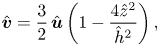 \begin{gather} \hat{\boldsymbol{v}} = \frac{3}{2}\,\hat{\boldsymbol{u}}\left(1-\frac{4\hat{z}^2}{\hat{h}^2}\right), \end{gather}
 \begin{gather}\hat{\boldsymbol{\nabla}}\boldsymbol{\cdot}\hat{\boldsymbol{u}}= 0, \end{gather}
 \begin{gather}\hat{\boldsymbol{u}} ={-}\frac{\hat{h}^2}{12\hat{\mu}}\,\hat{\boldsymbol{\nabla}} \hat{p}. \end{gather}
Here,  $\hat {\boldsymbol {v}}(\hat {x},\hat {y},\hat {z})$ is the full fluid velocity profile, $\hat {\boldsymbol {u}}(\hat {x},\hat {y})$ is the depth-averaged fluid velocity, $\hat {z} \in [-\hat {h}/2,\hat {h}/2]$ denotes the height coordinate, $\hat {p}(\hat {x},\hat {y})$ is the leading-order pressure, and $\hat {\mu }$ is the fluid viscosity.
In this subsection, we focus on the simple model problem of a single bubble in a large cell with a prescribed uniform background flow of speed  $\hat {U}$ in the $\hat {x}$-direction, which gives us the far-field condition
 \begin{equation} \hat{\boldsymbol{u}}\rightarrow \hat{U}\boldsymbol{i} \quad \text{as}\ \hat{x}^2 + \hat{y}^2 \rightarrow \infty, \end{equation}
where  $\boldsymbol {i}$ is the unit vector in the $\hat {x}$-direction.
Looking down on the cell from above (figure 1a), the boundary of the bubble appears to be a closed curve in the  $(\hat {x},\hat {y})$-plane, on which we impose the effective boundary conditions (Meiburg Reference Meiburg1989)
 \begin{gather} \boldsymbol{n}\boldsymbol{\cdot} \hat{\boldsymbol{u}} = \hat{U}_n, \end{gather}
 \begin{gather}\hat{p}_b - \hat{p} = \frac{2\hat{\gamma} }{\hat{h}} +\frac{2\hat{\gamma} }{\hat{h}}\,\beta({Ca}_{n})\,{Ca}_{n}^{2/3} + \frac{\hat{\gamma} {\rm \pi}}{4}\,\hat{\kappa}. \end{gather}
Here,  $\boldsymbol {n}$, $\hat {U}_n$ and $\hat {\kappa }$ are the outward-pointing normal, normal velocity and curvature of the apparent bubble boundary, respectively; $\hat {\gamma }$ is the surface-tension parameter, $\hat {p}_b$ is the uniform pressure inside the bubble, ${Ca}_n = \hat {\mu } \hat {U}_n/\hat {\gamma }$ is the capillary number based on the normal velocity, and $\beta$ is the Bretherton coefficient, whose value depends on whether the meniscus is advancing or retreating (Bretherton Reference Bretherton1961; Wong, Radke & Morris Reference Wong, Radke and Morris1995; Halpern & Jensen Reference Halpern and Jensen2002):
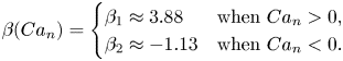 \begin{equation} \beta({Ca}_n)=\begin{cases} \beta_1 \approx 3.88 & \text{when }{Ca}_n > 0,\\ \beta_2 \approx{-}1.13 & \text{when }{Ca}_n < 0. \end{cases} \end{equation}
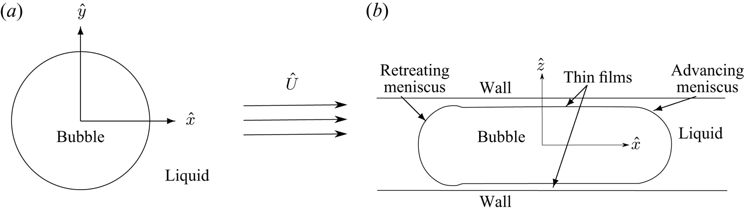
Figure 1. (a) Plan view of a bubble in a Hele-Shaw cell with a uniform background flow of speed  $\hat {U}$. (b) Side view of the bubble.
The first term on the right-hand side of (2.3b) is the capillary pressure difference due to the meniscus at the bubble boundary, whose leading-order radius of curvature is given by  $\hat {h}/2$. The second term, containing the capillary number, is the correction to the pressure difference in the limit ${Ca}_n\ll 1$, derived in Bretherton's original paper (Bretherton Reference Bretherton1961), due to the existence of the thin-film regions between the bubble and the walls of the cell (see figure 1b). The final term in (2.3b) captures the in-plane contribution to the curvature of the bubble interface, including the ${\rm \pi} /4$ factor derived by Park & Homsy (Reference Park and Homsy1984).
We will discuss further the underlying assumptions and validity of the boundary condition (2.3b) in § 4.
2.2. Non-dimensionalisation
We non-dimensionalise the model (2.1)–(2.3), scaling lengths with a typical bubble radius  $\hat {R}$, and velocities with the far-field uniform flow speed $\hat {U}$. We also scale $\hat {p}$ with $12\hat {\mu }\hat {U}R/{\hat {h}}^2$, $\hat {p}_b$ with $2\hat {\gamma } / \hat {h}$, and $\hat {\kappa }$ with $1/\hat {R}$. This process yields the following dimensionless system (in which dimensionless variables are denoted without hats):
 \begin{gather} \nabla^2 p = 0 \quad \mbox{in} \ \varOmega, \end{gather}
 \begin{gather}p_b - \frac{3\,{Ca}}{\epsilon}\,p = 1 + {Ca}^{2/3}\,\beta(U_n)\,U_n^{2/3} + \frac{\epsilon {\rm \pi}}{4}\,\kappa \quad \mbox{on} \ \partial \varOmega_b, \end{gather}
 \begin{gather}\boldsymbol{n}\boldsymbol{\cdot} \boldsymbol{\nabla} p={-} U_n \quad \mbox{on}\ \partial \varOmega_b, \end{gather}
 \begin{gather}p\sim{-}x+o(1) \quad \text{as} \ x^2 +y^2 \rightarrow \infty, \end{gather}
where  $\varOmega$ is the fluid domain, and $\partial \varOmega _b$ is the apparent bubble–fluid boundary in the $(x,y)$-plane, whose normal velocity is $U_n$. The far-field condition (2.5d) (with no logarithmic contribution) enforces conservation of the bubble area and thus in principle allows the bubble pressure $p_b$ to be determined as part of the solution.
The system (2.5) contains two dimensionless parameters, the aspect ratio and the capillary number, defined by
 \begin{equation} \epsilon = \frac{\hat{h}}{2\hat{R}}, \quad {Ca} = \frac{\hat{\mu} \hat{U}}{\hat{\gamma}}, \end{equation}
respectively. For the boundary-value problem (2.5) to be valid, both of these parameters must be small: the Hele-Shaw model relies on  $\epsilon$ being small, while the boundary condition (2.3b) is an asymptotic approximation in the limit ${Ca}\rightarrow 0$ (Park & Homsy Reference Park and Homsy1984). In the boundary condition (2.5b), the dominant balance depends on the relative size of these two small parameters.
In this work, we study flows in which the Hele-Shaw pressure is of the same order as the Bretherton drag term, and (2.5b) shows that this occurs when  ${Ca} = O(\epsilon ^3)$. Expanding $p_b$ and $\kappa$ as asymptotic expansions in powers of $\epsilon$, we then see that
 \begin{align} p_{b_0}+\epsilon p_{b_1} + \epsilon^2 p_{b_2} -\underbrace{\frac{3\,{Ca}}{\epsilon}\,p}_{O (\epsilon^2)}\ +\ O(\epsilon^3) \sim 1 + \frac{\epsilon {\rm \pi}}{4}\, (\kappa_0+\epsilon\kappa_1) + \underbrace{\beta\,{Ca}^{2/3}\,U_n^{2/3}}_{O(\epsilon^2)}\ +\ O(\epsilon^3) \end{align}
on  $\partial \varOmega _b$. At $O(1)$, we find that $p_{b_0} = 1$, indicating that the leading-order bubble pressure is determined by the capillary pressure jump across the meniscus. At $O(\epsilon )$, we obtain $\kappa _0=4p_{b_1}/{\rm \pi} = \text {const.}$, which implies that the bubbles that we are studying are circular to leading order in $\epsilon$. By our choice of length scale $\hat {R}$, we can take the bubble here to have unit dimensionless radius.
Since the bubble remains (approximately) circular for all time, the normal velocity on the boundary is just given by  $U_n=\boldsymbol {U}_b\boldsymbol {\cdot }\boldsymbol {n}$, where $\boldsymbol {U}_b=(U_b,V_b)$ is the constant bubble velocity. In terms of plane polar coordinates $(r,\theta )$ based on the bubble centre, we therefore find that the pressure in the liquid satisfies the problem
 \begin{gather} \nabla^2 p = 0 \quad \mbox{in} \ r>1, \end{gather}
 \begin{gather}\frac{\partial p}{\partial r} ={-}\boldsymbol{U}_b\boldsymbol{\cdot}\boldsymbol{n}={-}U_b\cos\theta-V_b\sin\theta\quad \mbox{on} \ r=1, \end{gather}
 \begin{gather}p\sim{-}r\cos\theta+o(1) \quad \text{as} \ r \rightarrow \infty. \end{gather}
 If  $\boldsymbol {U}_b$ were known, then $p$ would be uniquely determined by (2.8). To find the bubble velocity, we return to the boundary condition (2.7), which so far has been imposed up to $O(\epsilon )$. In principle, the solvability condition at $O(\epsilon ^2)$ determines $\boldsymbol {U}_b$ and closes the problem. As a shortcut to deriving this condition, we note that for any smooth closed planar curve $\partial \varOmega _b$ and with $\boldsymbol {k}$ denoting the unit vector in the $z$-direction,
 \begin{equation} \oint_{\partial\varOmega_b} \boldsymbol{n} \, \mathrm{d}s= {\oint_{\partial\varOmega_b} \boldsymbol{k}\times\frac{\mathrm{d}\boldsymbol{r}}{\mathrm{d}s} \, \mathrm{d}s= \boldsymbol{0},\quad} \oint_{\partial\varOmega_b} \kappa \boldsymbol{n} \, \mathrm{d}s = \oint_{\partial\varOmega_b} -\frac{\mathrm{d}^2\boldsymbol{r}}{\mathrm{d}s^2} \, \mathrm{d}s= \boldsymbol{0}, \end{equation}
by standard results from differential geometry (see e.g. Kreyszig Reference Kreyszig1959, Chapter 2). We therefore obtain from (2.5b) the constraint
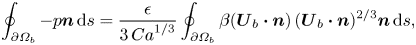 \begin{equation} \oint_{\partial\varOmega_b} -p\boldsymbol{n}\, \mathrm{d}s = \frac{\epsilon}{3\,{Ca}^{1/3}} \oint_{\partial\varOmega_b} \beta (\boldsymbol{U}_{b} \boldsymbol{\cdot} \boldsymbol{n})\,(\boldsymbol{U}_{b} \boldsymbol{\cdot} \boldsymbol{n})^{2/3}\boldsymbol{n}\, \mathrm{d}s, \end{equation}
which may be interpreted as a force balance on the bubble. To evaluate the integral on the right-hand side of (2.10), we now use the fact that, to leading order, the boundary  $\partial \varOmega _b$ is the unit circle, which we parametrise using
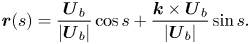 \begin{equation} \boldsymbol{r}(s)=\frac{\boldsymbol{U}_b}{|\boldsymbol{U}_b|}\cos s +\frac{\boldsymbol{k}\times\boldsymbol{U}_b}{|\boldsymbol{U}_b|}\sin s. \end{equation}
With  $\beta$ given by (2.4), we thus obtain
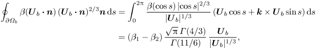 \begin{align} \oint_{\partial\varOmega_b} \beta (\boldsymbol{U}_{b} \boldsymbol{\cdot} \boldsymbol{n})\,(\boldsymbol{U}_{b} \boldsymbol{\cdot} \boldsymbol{n})^{2/3}\boldsymbol{n}\, \mathrm{d}s &= \int_0^{2{\rm \pi}} \frac{\beta(\cos s)\,|{\cos s}|^{2/3}}{|\boldsymbol{U}_b|^{1/3}} \left(\boldsymbol{U}_b\cos s+\boldsymbol{k}\times\boldsymbol{U}_b\sin s\right)\mathrm{d}s\nonumber\\ &=(\beta_1-\beta_2)\,\frac{\sqrt{\rm \pi}\,\varGamma(4/3)}{\varGamma(11/6)}\, \frac{\boldsymbol{U}_b}{|\boldsymbol{U}_b|^{1/3}}, \end{align}
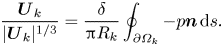
where  $\varGamma$ denotes the gamma function. Thus (2.10) reduces to the following condition for the bubble velocity:
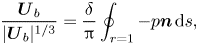 \begin{equation} \frac{\boldsymbol{U}_b}{|\boldsymbol{U}_b|^{1/3}} =\frac{\delta}{\rm \pi}\oint_{r=1} -p\boldsymbol{n}\, \mathrm{d}s, \end{equation}
where we define the Bretherton parameter
 \begin{equation} \delta = \frac{3\sqrt{\rm \pi}\,\varGamma(11/6)}{(\beta_1 - \beta_2)\,\varGamma(4/3)}\, \frac{{Ca}^{1/3}}{\epsilon} \approx 1.12\,\frac{{Ca}^{1/3}}{\epsilon}. \end{equation}
By assumption,  $\delta$ is $O(1)$ while $\epsilon$ and ${Ca}$ are asymptotically small.
2.3. Solution
The problem (2.8) for an isolated circular bubble in an infinite cell is easily solved to obtain the pressure
 \begin{equation} p = \left(\frac{U_b -1}{r}-r\right)\cos\theta + \frac{V_b}{r}\sin\theta. \end{equation}
We can thus evaluate the integral on the right-hand side of the force balance (2.12) to obtain an equation for the bubble velocity, namely
 \begin{equation} \frac{\boldsymbol{U}_b}{|\boldsymbol{U}_b|^{1/3}}=\delta(2\boldsymbol{i}-\boldsymbol{U}_b). \end{equation}
It follows that the bubble moves parallel to the background flow, as expected, with  $\boldsymbol {U}_b=U_b\boldsymbol {i}$, where $U_b$ satisfies the algebraic equation
 \begin{equation} \frac{U_b^{2/3}}{2-U_b}=\delta.\end{equation}
The equation (2.16) for the bubble speed is equivalent to that found in Reichert et al. (Reference Reichert, Cantat and Jullien2019), using a laborious viscous dissipation argument. (In Reichert et al. (Reference Reichert, Cantat and Jullien2019), the constant of proportionality in (2.13) is found to be 1.20 rather than 1.12, due to inaccurate calculation of the integral and the Bretherton constants. Their method involves solution for the height of the thin liquid films above and below the bubble, followed by calculation of the viscous dissipation due to the thin films.) We note that (2.16) may be transformed into a cubic and thus solved explicitly for  $U_b$; however, the resulting expression is unwieldy and not particularly illuminating.
We plot the prediction (2.16) for the bubble velocity  $U_b$ versus the Bretherton parameter $\delta$ in figure 2, which shows good agreement with experimental data taken from Reichert et al. (Reference Reichert, Cantat and Jullien2019) and Park et al. (Reference Park, Maruvada and Yoon1994). We observe that $U_b$ is an increasing function of $\delta$; from (2.13), we see that $\delta$ is proportional to the bubble radius $\hat {R}$, which implies that larger bubbles should travel faster. As $\delta \rightarrow 0$, the Bretherton drag term dominates and $U_b \sim (2\delta )^{3/2}$. At the other extreme, where $\delta \gg 1$, we recover the traditional Taylor–Saffman result (Taylor & Saffman Reference Taylor and Saffman1959) of the bubble moving twice as fast as the outer flow. However, we note that the assumption of the bubble remaining approximately circular eventually fails if $\delta$ is too large. From (2.7), we observe that variations in the bubble curvature are of order $\delta ^2\epsilon$, which is assumed to be small. We conclude that our model remains valid when $\delta$ is large, provided that $1\ll \delta \ll \epsilon ^{-1/2}$.
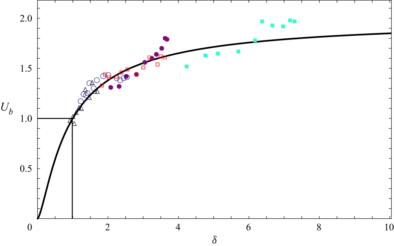
Figure 2. The ratio  $U_b$ of the bubble velocity to the outer fluid velocity as a function of the Bretherton parameter $\delta$. The solid curve shows the model prediction (2.16). The points show experimental data: cyan solid squares ( $\epsilon =0.035$) and maroon solid dots ( $\epsilon = 0.071$) from Park et al. (Reference Park, Maruvada and Yoon1994), with ${Ca}$ in the range $2.3\unicode{x2013}12.7\times 10^{-3}$; red squares ( $\epsilon = 0.044)$, blue circles ( $\epsilon = 0.07$) and grey triangles ( $\epsilon = 0.091$) from Reichert et al. (Reference Reichert, Cantat and Jullien2019), with ${Ca}$ in the range $0.4\unicode{x2013}6.0\times 10^{-3}$.
From (2.16), we observe a transition in behaviour at  $\delta = 1$: if $\delta < 1$, then the bubble moves slower than the outer flow ( $U_b<1)$, while if $\delta > 1$, then the bubble moves faster than the outer flow ( $U_b>1)$. The critical case where $U_b=1$, so the bubble moves with the external flow, corresponds to the particular solution of the problem where $p \equiv -x$. We see that this solution satisfies (2.8) provided that $(U_b,V_b) = (1,0)$, and the force balance (2.12) is also satisfied provided that $\delta = 1$.
2.4. The  $N$-bubble problem

It is straightforward to generalise the model derived above to describe a system of  $N$ bubbles. For the moment, we continue to treat the Hele-Shaw cell containing the bubbles as effectively infinite, with a uniform flow imposed at infinity; the effects of cell boundaries will be incorporated below.
As in § 2.2, each bubble remains circular (to leading order), with dimensionless radius  $R_k$ and velocity $\boldsymbol {U}_k$, say, for $1\leqslant k\leqslant N$. The dimensionless pressure in the liquid domain $\varOmega$ therefore satisfies
 \begin{gather} \nabla^2 p = 0 \quad \text{in} \ \varOmega, \end{gather}
 \begin{gather}\boldsymbol{n}\boldsymbol{\cdot}\boldsymbol{\nabla} p ={-}\boldsymbol{U}_{k} \boldsymbol{\cdot} \boldsymbol{n} \quad\text{on} \ \partial\varOmega_{k}, \end{gather}
 \begin{gather}\boldsymbol{\nabla}p\rightarrow-\boldsymbol{i} \quad \text{as} \ x^2 +y^2 \rightarrow \infty, \end{gather}
where  $\partial \varOmega _{k}$ denotes the (circular) boundary of the $k\text {th}$ bubble. In principle, $p$ would thus be determined if we knew the velocity $\boldsymbol {U}_k$ of each bubble. Indeed, the boundary-value problem described in (2.17) would then be equivalent to finding the velocity potential exterior to a collection of moving bodies or stirrers in two-dimensional irrotational flow with no circulation. The two-body version of this problem has been solved by Tchieu, Crowdy & Leonard (Reference Tchieu, Crowdy and Leonard2010), and general integral expressions for the velocity potential due to any finite number of moving bodies are given by Crowdy (Reference Crowdy2008).
In the present problem, however, the bubble velocities are not known in advance. As in § 2.2, the required equation of motion is obtained by performing an effective force balance, which here leads to
 \begin{equation} \frac{\boldsymbol{U}_k}{|\boldsymbol{U}_k|^{1/3}} =\frac{\delta}{{\rm \pi} R_k}\oint_{\partial\varOmega_k} -p\boldsymbol{n}\, \mathrm{d}s. \end{equation}
 Again we notice that  $p = -x$ is a solution to the problem (2.17) if and only if all of the bubbles move at the same velocity $\boldsymbol {U}_k =\boldsymbol {i}$ for all $k$. The force balance (2.18) then requires $\delta R_k=1$. Therefore, it is possible for all of the bubbles to be convected at the same velocity as the outer flow, regardless of their position, only when all the bubbles are the same size.
Thus far we have formulated a general model for the motion of approximately circular bubbles in a Hele-Shaw cell, and solved the model explicitly for the simplest possible case of a single isolated bubble. In the next section, we use the model to analyse some more complicated examples, which illustrate the effects of walls on the bubble motion and the interactions between multiple bubbles.
3. Examples
3.1. Isolated bubble near a wall
Next, we consider the case of a single bubble in a semi-infinite Hele-Shaw cell ( $y>0$) with an impermeable wall at $y=0$ and a uniform flow $-\boldsymbol {\nabla }p\sim \boldsymbol {i}$ at infinity. The bubble is taken to have unit dimensionless radius, with its centre a dimensionless distance $a>1$ away from the boundary. The following analysis allows us to examine how proximity to a wall affects the velocity of the bubble, and also illustrates the application of complex variable methods to our model. This formulation is equivalent to the problem of two identical bubbles in an infinite cell with their centres separated by $2a$ and lined up perpendicular to the outer flow direction, with the wall representing the line of symmetry between them. The corresponding two-bubble problem was solved by Sarig et al. (Reference Sarig, Starosvetsky and Gat2016) using bipolar coordinates rather than complex variables. We choose the bubble centre to be instantaneously at $z = x+\mathrm {i}y=a\mathrm {i}$, so that the domain of interest is $\varOmega =\{z: \operatorname {Im}(z)>0, |z-a\mathrm {i}|>1\}$.
Since  $p$ satisfies Laplace's equation, we introduce a complex potential $w(z) = -p + \mathrm {i}\psi$, where $\psi$ is the streamfunction. The problem is then to find a holomorphic function $w(z)$ in the region $\varOmega$ such that
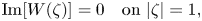
 \begin{gather} \operatorname{Im}[w(z)] = 0 \quad \text{on} \ \operatorname{Im}(z) = 0, \end{gather}
 \begin{gather}\operatorname{Im}[w(z)] = q +\operatorname{Im}\left[\bar{\mathcal{U}}_bz\right] \quad\text{on} \ |z-a\mathrm{i}|=1, \end{gather}
 \begin{gather}w(z) \sim z \quad\text{as} \ z \rightarrow \infty {.} \end{gather}
Both the complex bubble velocity  $\mathcal {U}_b=U_b+\mathrm {i}V_b$ and the real constant $q$ are a priori unknown; $q$ represents the flux of liquid through the gap between the bubble and the wall (relative to the moving bubble). Once we have solved for $w$, the equation of motion (2.12) may be imposed by evaluating
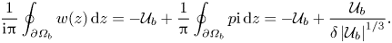 \begin{equation} \frac{1}{\mathrm{i}{\rm \pi}}\oint_{\partial\varOmega_b} w(z)\,\mathrm{d}z={-}\mathcal{U}_b+\frac{1}{\rm \pi}\oint_{\partial\varOmega_b}p\mathrm{i}\,\mathrm{d}z ={-}\mathcal{U}_b+\frac{\mathcal{U}_b}{\delta\left|\mathcal{U}_b\right|^{1/3}}. \end{equation}
 We proceed by conformally mapping  $\varOmega$ onto a concentric annulus, where the problem becomes solvable with standard techniques. Following the mapping
 \begin{equation} \zeta = f(z) = \frac{z-\mathrm{i}\sqrt{a^2-1}}{z+\mathrm{i}\sqrt{a^2-1}}, \end{equation}
the solution domain in the  $\zeta$-plane is $A=\{\zeta :X<|\zeta |<1\}$, where
 \begin{equation} X =a-\sqrt{a^2-1}. \end{equation}
Writing the complex potential in the form  $w(z)= z+W(f(z))$, we find that $W$ is holomorphic on $A$ and satisfies the boundary conditions
 \begin{gather} \operatorname{Im}[W(\zeta)] = 0 \quad \text{on} \ |\zeta| = 1, \end{gather}
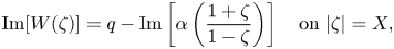 \begin{gather}\operatorname{Im}[W(\zeta)] = q- \operatorname{Im}\left[\alpha\left(\frac{ 1+\zeta}{1-\zeta}\right)\right] \quad\text{on}\ |\zeta| = X, \end{gather}
where  $\alpha = (1-\bar {\mathcal {U}}_b)\mathrm {i}\sqrt {a^2-1}$.
We then find that the a priori unknown flux  $q$ is given by
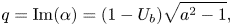 \begin{equation} q=\operatorname{Im}(\alpha)= (1-U_b)\sqrt{a^2-1}, \end{equation}
and the complex potential in the  $\zeta$-plane is given by
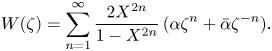 \begin{equation} W(\zeta) = \sum_{n=1}^{\infty}\frac{2 X^{2n}}{1 - X^{2n}}\,(\alpha\zeta^n+\bar{\alpha}\zeta^{{-}n}). \end{equation}
We can thus calculate the integral on the left-hand side of (3.2) by transforming into the  $\zeta$-plane and then using Cauchy's residue theorem to obtain
 \begin{equation} \frac{1}{\mathrm{i}{\rm \pi}}\oint_{\partial\varOmega_b} w(z) \, \mathrm{d}z = \frac{2\sqrt{a^2 -1}}{\rm \pi}\oint_{|\zeta| = X} \frac{W(\zeta)}{(\zeta -1)^2} \, \mathrm{d}\zeta = (1-\mathcal{U}_b)\,F(a), \end{equation}
where
 \begin{equation} F(a)=8(a^2-1)\sum_{n=1}^{\infty} \frac{n X^{2n}}{1 - X^{2n}}, \end{equation}
with  $X$ given as a function of $a$ by (3.4). The formula (3.9) may be written in closed form as
 \begin{equation} F(a) = 2(a^2 -1)\,\frac{\varPsi_{X^2}'(1)}{\log^2X}, \end{equation}
in which  $\varPsi _{X^2}$ denotes the $q$-digamma function (Salem Reference Salem2012), defined by
 \begin{equation} \varPsi_q (z)= \frac{1}{\varGamma_q (z)}\,\frac{\mathrm{d}\varGamma_q (z)}{\mathrm{d}z}, \end{equation}
where  $\varGamma _q$ is the $q$-gamma function (Askey Reference Askey1978). As shown in figure 3, $F(a)$ is a decreasing function of $a$, with $F(1) = {\rm \pi}^2 /3$ and $F(a) \rightarrow 2$ as $a\rightarrow \infty$.
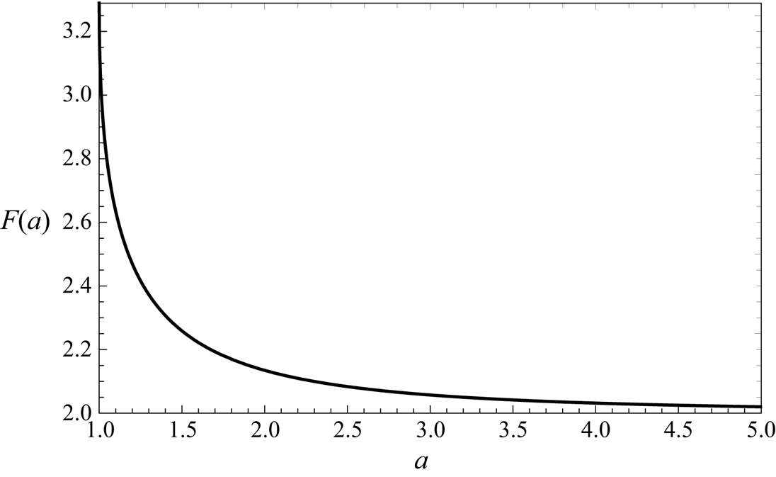
Figure 3. The function  $F(a)$ defined by (3.10).
Comparing imaginary parts in (3.2), we find that  $V_b = 0$, so the bubble moves parallel to the wall. Then equating real parts in (3.2), the bubble's velocity in the $x$-direction is found to satisfy the algebraic equation
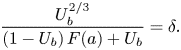 \begin{equation} \frac{U_b^{2/3} }{ (1-U_b)\,F(a)+U_b}= \delta. \end{equation}
Once again, (3.12) gives us a cubic that in principle can be solved explicitly for the dimensionless bubble velocity  $U_b$. Rather than writing this complicated expression out explicitly, below we briefly examine the possible limiting cases.
First, we observe that  $U_b =1$ when $\delta = 1$, so the bubble moves precisely with the external flow at this same critical value of the Bretherton parameter, regardless of the distance from the wall. As noted in § 2.3, this special case corresponds to the particular solution where $p = -x$. For the extreme values of the Bretherton parameter $\delta$, using (3.12) we derive the limits
 \begin{gather} U_b \rightarrow \frac{F(a)}{F(a)-1} \quad\text{as}\ \delta \rightarrow \infty, \end{gather}
 \begin{gather}U_b \sim \left(\delta\,F(a)\right)^{3/2} \quad\text{as}\ \delta \rightarrow 0. \end{gather}
Taking the derivative of (3.12) with respect to  $\delta$, we find
 \begin{equation} \frac{\partial U_b}{\partial \delta} =\frac{3U_b}{\delta\left[3\delta\left(F(a)-1\right)U_b^{1/3}+2\right]}>0, \end{equation}
so  $U_b$ is a strictly increasing function of $\delta$. It follows that $U_b >1$ when $\delta > 1$, and vice versa.
As noted above,  $F(a) \rightarrow 2$ as $a \rightarrow \infty$, so in this limit, (3.12) reduces to the result (2.16) for a bubble in an infinite fluid medium, as expected. Similarly, we can look at the limit $a\rightarrow 1$ in which the bubble touches the wall. Since $F(1) = {\rm \pi}^2 / 3$, the bubble velocity tends to a non-zero value, which depends on the Bretherton parameter through the relation
 \begin{equation} \frac{3U_b^{2/3}}{{\rm \pi}^2 - ({\rm \pi}^2 -3)U_b}=\delta. \end{equation}
For intermediate values of  $a$, we find that
 \begin{equation} \frac{\partial U_b}{\partial a} = \left[\frac{-\delta\,F'(a)}{\delta(F(a)-1)+\frac{2}{3} U_b^{{-}1/3}}\right](U_b-1), \end{equation}
in which the term in square brackets is positive. It follows that  $U_b$ is a decreasing function of $a$ when $\delta < 1$, but an increasing function of $a$ when $\delta > 1$.
The behaviour of the bubble velocity as the parameters  $a$ and $\delta$ are varied is shown in figure 4. As predicted, we observe that the presence of the wall either increases or decreases the bubble velocity, depending on whether $\delta <1$ or $\delta >1$, respectively. At the critical value $\delta = 1$, we have $U_b =1$ and the distance from the wall no longer matters.
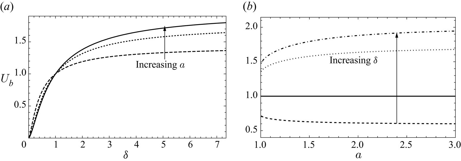
Figure 4. (a) Bubble velocity  $U_b$ versus Bretherton parameter $\delta$ for $a = 1$ (dashed), $a = 1.5$ (dotted) and $a = \infty$ (solid). (b) Bubble velocity $U_b$ versus distance $a$ from the wall for Bretherton parameter $\delta = 1/2$ (dotted), $\delta = 1$ (solid), $\delta = 5$ (dashed) and $\delta = \infty$ (dot-dashed).
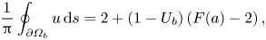
At first glance, it appears paradoxical that proximity to the wall may cause the bubble to either speed up or slow down, depending on the size of  $\delta$, but the behaviour may be explained as follows. By using the boundary condition (2.17b) and integration by parts, the force balance (2.18) may be rewritten as
 \begin{equation} \boldsymbol{U}_b\left(1+ \frac{1}{\delta\,|\boldsymbol{U}_b|^{1/3}}\right) =\frac{1}{\rm \pi}\oint_{\partial\varOmega_b} \boldsymbol{u}\, \mathrm{d}s, \end{equation}
where  $\boldsymbol {u}=(u,v)^{\text {T}}=-\boldsymbol {\nabla }p$ is the dimensionless liquid velocity. For an isolated bubble, with the pressure given by (2.14), the integral on the right-hand side of (3.17) is easily calculated to be $2\boldsymbol {i}$, reproducing the equation of motion (2.15), and in general this term captures the influence of the outer flow on the bubble motion.
Now, what happens when a wall is introduced next to the moving bubble? From (3.6), we can calculate the average flow speed through the gap between the bubble and the wall (relative to the moving bubble) as
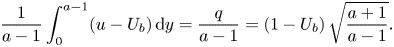 \begin{equation} \frac{1}{a-1}\int_0^{a-1}(u-U_b)\,\mathrm{d} y= \frac{q}{a-1}=(1-U_b)\,\sqrt{\frac{a+1}{a-1}}. \end{equation}
First, suppose that the bubble is moving more slowly than the external flow, so  $U_b<1$. The right-hand side of (3.18) increases as the separation $a-1$ between the bubble and the wall decreases, measuring the acceleration of the liquid as it squeezes between the bubble and the wall. We find that the average velocity on the bubble surface thus increases and, according to (3.17), the bubble velocity also increases (relative to an isolated bubble). The horizontal component of the right-hand side of (3.17) may be calculated as
 \begin{equation} \frac{1}{\rm \pi}\oint_{\partial\varOmega_b}u\,\mathrm{d}s =2+(1-U_b)\left(F(a)-2\right), \end{equation}
which indeed increases as  $a$ decreases when $U_b<1$.
On the other hand, if the bubble moves more quickly than the external flow ( $U_b>1$), then the liquid is squeezed backwards through the gap between the bubble and the wall so, by the same argument, the integral on the right-hand side of (3.17) and the bubble velocity should both decrease. This physical reasoning indeed agrees with the behaviour observed in figure 4. As noted above, the bubble travels faster or slower than the external flow depending on whether $\delta <1$ or $\delta >1$, and the effect of proximity to the wall is accordingly either to speed up or to slow down the bubble.
3.2. Isolated bubble in a channel
Next, we consider the motion of a singular bubble of unit radius in a Hele-Shaw channel of width  $W>2$, between impermeable walls at $y=\pm W/2$. We again impose a uniform flow with $p\sim -x$ at infinity and, without loss of generality, take the bubble centre to be instantaneously at $(x,y) = (0,y_b)$, where $|y_b|< W/2-1$. It may then be shown that $p$ is an odd function of $x$, and it follows from (2.12) that $V_b = 0$. Thus a single bubble in a channel will continue moving parallel to the outer flow no matter where in the channel it is initially placed.
To facilitate numerical solution, we pose the problem in terms of the streamfunction  $\psi$, which satisfies Dirichlet boundary conditions
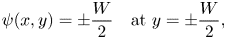 \begin{gather} \psi(x,y)={\pm}\frac{W}{2} \quad\text{at}\ y={\pm}\frac{W}{2}, \end{gather}
 \begin{gather}\psi(x,y)=q+U_b y \quad \text{at}\ x^2+(y-y_b)^2=1, \end{gather}
 \begin{gather}\psi(x,y)\rightarrow y \quad \text{as}\ x\rightarrow\pm\infty. \end{gather}
The a priori unknown constant  $q$ is in principle determined by the constraint
 \begin{equation} \oint_{\partial\varOmega_b}\frac{\partial\psi}{\partial n}\,\mathrm{d}s=0, \end{equation}
which follows from single-valuedness of the pressure. The streamfunction is then decomposed as  $\psi =U_b y+(1-U_b)\psi _1+q\psi _2$, where each $\psi _k$ satisfies a normalised boundary-value problem that is independent of $q$ and $U_b$. We solve for $\psi _1$ and $\psi _2$ using finite element methods, and then compute the four integrals
 $$\begin{gather} I_k=\frac{1}{\rm \pi}\oint_{\partial\varOmega_b}\left(\frac{\partial\psi_k}{\partial x}\,\mathrm{d}y- \frac{\partial\psi_k}{\partial y}\,\mathrm{d} x\right), \end{gather}$$
 $$\begin{gather}J_k=\frac{1}{\rm \pi}\oint_{\partial\varOmega_b}\left(x\,\frac{\partial\psi_k}{\partial x}+(y-y_b)\,\frac{\partial\psi_k}{\partial y}\right)\mathrm{d} x \end{gather}$$
( $k=1,2$). The force balance (2.12) and constraint (3.21) provide two algebraic equations for $q$ and $U_b$. As in § 3.1, the resulting equation of motion may be expressed in the form
 \begin{equation} \frac{U_b^{2/3}}{(1-U_b)\,F(W,y_b)+U_b}=\delta, \end{equation}
where now  $F(W,y_b)=J_2I_1/I_2-J_1$. For given values of $W$ and $y_b$, the value of $F(W,y_b)$ can be computed once-and-for-all, following the procedure described above, and the dependence of $U_b$ on $\delta$ is then determined by (3.23). An analogous approach is used to compute the numerical solutions with multiple bubbles below.
We start by considering a bubble travelling along the centreline of the channel, with  $y_b=0$, in which case it is easy to see that $q$ must also equal zero. Hence $F(W,0)=-J_1$, and the one remaining integral can in principle be calculated using a Schwarz–Christoffel mapping (Anselmo et al. Reference Anselmo, Nelson, Carneiro da Cunha and Crowdy2018) or approximation schemes described by Crowdy (Reference Crowdy2016) and Love (Reference Love1938), for example.
In figure 5(a), we examine the effects of varying the channel width  $W$ and Bretherton parameter $\delta$. We observe that $U_b$ is an increasing function of $\delta$, and as $\delta \rightarrow \infty$, it tends to a value strictly less than the Taylor–Saffman value $U_b=2$. Again $\delta = 1$ is the critical value where the bubble moves with the external flow independently of the channel width, corresponding to the exact solution of the problem where $p=-x$. As in § 3.1, the bubble may be accelerated or retarded by the presence of walls, depending on whether $\delta <1$ or $\delta >1$, respectively. In the limit of large $W$, the solution approaches that for an isolated bubble, as expected, while the solutions all converge to $U_b=1$ as $W\rightarrow 2$. This latter limit corresponds to the case when the bubble exactly fits the channel width and, by conservation of mass, must travel at the same speed as the outer flow.

Figure 5. Bubble velocity  $U_b$ versus: (a) channel width $W$, with offset $y_b=0$; (b) distance $W/2-1-y_b$ from the top channel wall, with width $W=4$ and offset $y_b\in [0,1]$. Here, the Bretherton parameter is $\delta =1/2$ (dashed), $\delta =1$ (solid), $\delta = 5$ (dotted) and $\delta = \infty$ (dot-dashed).
In figure 5(b), we study the effects of the bubble being off-centre in the channel by fixing  $W=4$ and varying $y_b$. Again we observe that proximity to a wall may either increase or decrease the bubble velocity, depending on whether $\delta < 1$ or $\delta > 1$, respectively, with $\delta =1$ the critical case where $U_b=1$ for all $y_b$. As in § 3.1, this behaviour is caused by the liquid flowing through the gaps between the bubble and the channel walls, which either speeds up or slows down, thereby increasing or decreasing the average velocity at the bubble surface in (3.17).
3.3. Two identical bubbles in a channel
Next, we examine a system of two identical bubbles travelling along the centreline of the channel. Without loss of generality, we take the centres of the two bubbles to be initially at  $\pm (1+S/2,0)$, where $S$ is the bubble separation. By symmetry, one can then show that the bubbles must both move along the centreline with identical velocities $\boldsymbol {U}_1=\boldsymbol {U}_2=(U_b,0)$.
In figure 6, we show that the two-bubble solution converges rapidly to the corresponding one-bubble solution as we increase the separation between the two bubbles, with the solutions matching up very closely even for  $S=2$. For $\delta <1$, the bubble pair moves more slowly than a single bubble, but for $\delta >1$, it moves more quickly. In other words, the acceleration or retardation of the liquid as it squeezes through the gaps between each bubble and the channel walls (as described in §§ 3.1 and 3.2) is suppressed by the presence of the other bubble.
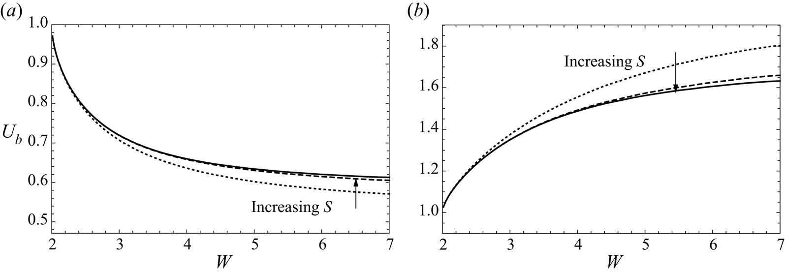
Figure 6. Bubble velocity  $U_b$ versus channel width $W$ for a two-bubble system with separation $S = 0.2$ (dotted), $S = 2$ (dashed), single-bubble solution (solid), and (a) $\delta = 1/2$, (b) $\delta =5$.
3.4. A Hele-Shaw Newton's cradle
With three identical bubbles moving along the centreline of a channel, we find that the bubbles in general have different speeds so, for the first time, we have to solve an unsteady problem. At each time step, we compute the three instantaneous bubble speeds by following an approach similar to that described in § 3.2, and then update the bubble positions. We again see different behaviour depending on whether  $\delta <1$ or $\delta >1$.
At the special value  $\delta =1$, all of the bubbles move with the background flow, so the distances between them remain fixed. When $\delta < 1$, the bubbles move more slowly than the surrounding liquid. In this case, we recall from § 3.3 that the bubbles’ speed is increased by confinement from the channel walls but decreased by the presence of a second bubble. When there are three bubbles, we find that the outer two bubbles shield the middle one from the accelerating influence of the walls. We therefore observe that the centre bubble moves backwards relative to the outer two, and thus eventually becomes a pair with the rear bubble (see figure 7a). This qualitative behaviour has been observed experimentally by Shen et al. (Reference Shen, Leman, Reyssat and Tabeling2014); however, there were surfactants in their system so a quantitative comparison with our model is not possible. The opposite effect occurs when $\delta >1$, where now the central bubble moves faster than the outer ones and so eventually joins with the front bubble (see figure 7b).

Figure 7. The progression of a series of three identical bubbles, with (a)  $\delta =1/2$, (b) $\delta =5$.
Figure 8 depicts the dependence on  $\delta$ of the time $T$ taken for the middle bubble either to be caught by the rear bubble or to catch the front bubble. The initial bubble separations are set to $1$ and $0.04$, as shown in figure 7(a) for $\delta <1$ and figure 7(b) for $\delta >1$, and we show the results for two channel widths, $W=4$ and $W=20$. We see an asymptote at $\delta =1$, as expected when all the bubbles travel at the outer fluid speed. There is also an asymptote as $\delta \rightarrow 0$, since the bubble velocities all tend to zero in this limit. As $\delta \rightarrow \infty$, $T$ approaches a finite non-zero value that depends on $W$. Furthermore, we observe that $T$ increases as we decrease the channel width, with $T\rightarrow \infty$ as $W\rightarrow 2$ for all values of $\delta$, again because the bubbles all move at the same speed in this limit, by conservation of mass. Even at $W=4$, the transit time is quite large for all values of $\delta$, indicating that the difference in speed between the bubbles is relatively small.
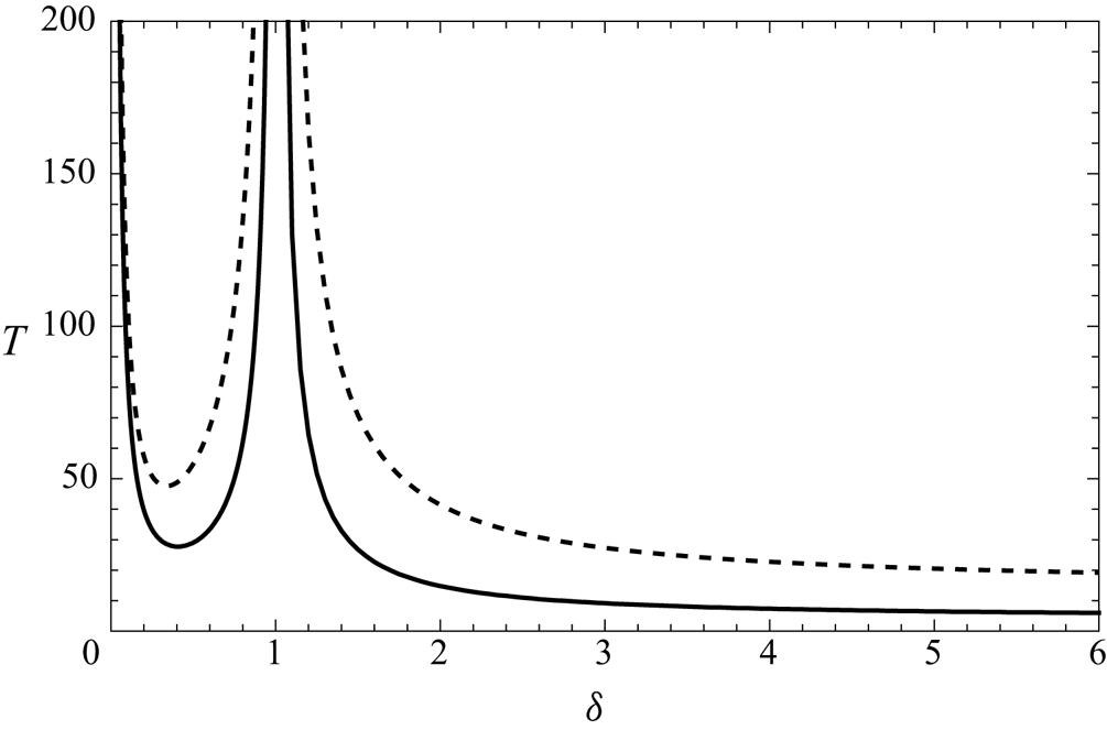
Figure 8. The transit time  $T$ versus Bretherton parameter $\delta$ for the system shown in figure 7(a) for $\delta <1$ and figure 7(b) for $\delta >1$, in a channel of width $W=20$ (solid) and $W=4$ (dashed). When $\delta <1$, the computation starts with separations of $1$ and $0.04$ between the rear two and front two bubbles, respectively, and finishes when the separation between the rear two bubbles is $0.04$; and vice versa when $\delta >1$.
When there are more than three bubbles, this effect can occur multiple times, as illustrated in figure 9(a) for a case with  $\delta <1$. Initially, the second bubble breaks away from the front one to form a pair with the third bubble, before that pair itself breaks up so the third and fourth bubbles can form a pair. For $\delta <1$, we recall from § 3.3 that a pair of bubbles moves more slowly than an isolated bubble, so for longer times, the trailing pair in figure 9(a) is left behind by the front two. Beatus et al. (Reference Beatus, Bar-Ziv and Tlusty2012) observed qualitatively similar longitudinal waves propagating backwards relative to the outer fluid flow in a series of bubbles on the centreline of a Hele-Shaw channel, which behaviour they termed the peloton effect. However, we find that the wave propagation can occur in either direction, depending on whether $\delta <1$ or $\delta >1$. Figure 9(b) shows a typical case with $\delta >1$, where the initial condition is the reverse of that in figure 9(a), and the observed evolutions are almost mirror images of each other. When $\delta >1$, a pair of bubbles travels faster than an isolated bubble, so eventually the front pair breaks away and leaves behind the other two bubbles.
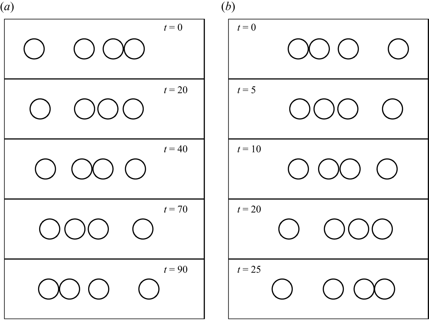
Figure 9. The progression of a series of four identical bubbles, with (a)  $\delta =1/2$, (b) $\delta =5$.
The formation and breakup of successive bubble pairs observed in figure 9 is highly reminiscent of a Newton's cradle, even though there is no inertia in our system, and the motion arises solely due to viscous hydrodynamic interactions.
4. Conclusions
In this paper, we develop a model for the motion of bubbles in a Hele-Shaw cell in the distinguished limit where the typical bubble aspect ratio  $\epsilon$ and capillary number ${Ca}$ satisfy ${Ca}^{1/3} = O(\epsilon ) \ll 1$. In this regime, each bubble remains approximately circular, and its velocity is determined by a net force balance. For an isolated bubble in an infinite Hele-Shaw cell, the model may be solved analytically, and the qualitative behaviour depends on a dimensionless ‘Bretherton parameter’, $\delta \propto {Ca}^{1/3}/\epsilon$. In particular, the bubble moves faster than the outer fluid speed when $\delta > 1$, slower when $\delta <1$, and precisely with the background flow if $\delta =1$.
As shown in figure 2, the theoretically predicted bubble velocity agrees quite well with the experimental literature, but we note that very little experimental data exists for the case  $\delta <1$. The regime with $\delta <1$ corresponds to ${Ca}\lesssim 0.7\epsilon ^3$, and with small values of the aspect ratio $\epsilon$ (as assumed in the Hele-Shaw theory), requires extremely small values of ${Ca}$. At such very low capillary numbers, the thin films between each bubble and the cell walls become so thin that other physical effects not included in the model (e.g. disjoining pressure) may become important, leading for example to film rupture. We believe that it is for this reason that the experiments at small values of $\delta$ usually include surfactants to stabilise the thin films. Our model does not at present capture the influence of surfactants on the bubble dynamics, though we note that some previous authors (e.g. Maruvada & Park Reference Maruvada and Park1996; Reichert et al. Reference Reichert, Cantat and Jullien2019) have tried to incorporate such effects in an ad hoc way.
When the effects of cell boundaries and multiple bubbles are included, we still observe striking changes in the qualitative behaviour depending on whether  $\delta$ is greater or less than $1$. For example, in a train of three identical bubbles travelling along a Hele-Shaw channel, we find that the middle bubble either catches up with the one in front (if $\delta >1$) or is caught by the one behind (if $\delta <1$). In longer bubble trains, we observe bubble pairs successively forming and breaking up from the front to the back of the train if $\delta <1$, or vice versa if ${\delta >1}$, resembling experimental observations by Beatus et al. (Reference Beatus, Bar-Ziv and Tlusty2012), for example. Although this behaviour is reminiscent of a Newton's cradle, it arises from long-range hydrodynamic interactions rather than through momentum transfer between the bubbles.
This phenomenon suggests that it is very difficult to maintain a finite stream of equally spaced identical bubbles moving along the centreline of a Hele-Shaw channel. The bubbles are always expected to bunch up into pairs or larger aggregates, unless we are in the special case where  $\delta =1$. We do find, though, that the relative bubble velocities are often quite small, so the clustering occurs quite slowly, and it may be minimised in experiments by reducing the channel width and by keeping $\delta$ as close to $1$ as possible (see figure 8). In future work, we will analyse the possible instability of bubble trains to lateral perturbations, as is also often seen in experiments (Beatus et al. Reference Beatus, Tlusty and Bar-Ziv2006; Shen et al. Reference Shen, Leman, Reyssat and Tabeling2014).
It can be shown that the equation of motion (2.18) allows bubbles to approach and touch cell boundaries or each other in finite time. In principle, our model breaks down when the distance between two bubbles (or between a bubble and a wall) becomes comparable with the cell thickness. However, it is often observed in experiments that bubbles can remain apparently stuck together without coalescing (Battat, Weitz & Whitesides Reference Battat, Weitz and Whitesides2022), and our model can easily be adapted to describe propagating pairs of bubbles that either remain attached or drift apart, depending on the sign of the mutual force between them.
We limit our attention in this paper to examples with relatively low numbers of equally sized and collinear bubbles. For a general system of  $N$ bubbles, our solution method would involve the numerical solution of $3N$ Dirichlet problems and computation of $9N^2$ force integrals to evaluate all of the bubble velocities at each time step. For large $N$, this approach can become very slow even when the unsteady phenomena described below are neglected. An attractive alternative approach is to assume that the bubbles are sufficiently well-spaced to be approximated by dipoles, as in Beatus et al. (Reference Beatus, Bar-Ziv and Tlusty2012) and Shen et al. (Reference Shen, Leman, Reyssat and Tabeling2014). In principle, dipole methods are valid only when the bubbles are well-separated; for two identical bubbles in an infinite Hele-Shaw cell, Green (Reference Green2018) found that the dipole approximation works well when the bubble separation is greater than about two bubble radii. It is the subject of current work to determine whether the dynamics that we observe (e.g. in figures 7 and 9) can be captured adequately by a dipole model, even when the bubbles become arbitrarily close and the dipole approach is not strictly valid.
Figure 2 shows that the speed of an isolated bubble is an increasing function of its radius. In examples with many non-identical bubbles, the dynamics depends on the relative sizes of neighbouring bubbles, as well as on the bubble interaction effects seen in figures 7 and 9, for example. In microfluidic experiments and devices, the bubble radii are often almost but not precisely uniform, and the resulting delicate balance between size effects and interaction effects is also the subject of current research.
As promised in § 2, we now discuss the validity of the boundary condition (2.3b). At the front interface of a moving bubble, the additional pressure drop (proportional to  ${Ca}_n^{2/3}$) may be derived by solving Bretherton's problem for a meniscus advancing with effective capillary number ${Ca}_n$ (Bretherton Reference Bretherton1961). As noted by Reichert et al. (Reference Reichert, Cantat and Jullien2019), this approach is invalid close to points where ${Ca}_n$ changes sign. Burgess & Foster (Reference Burgess and Foster1990) showed that the discontinuous term in (2.3b), involving the function $\beta$, is smoothed out in ‘lateral transition regions’ (LTRs) where ${Ca}_n=O(\epsilon ^{3/5}\,{Ca}^{1/5})$. In the distinguished limit studied here, ${Ca}$ is assumed to be of order $\epsilon ^3$, and it follows that the LTRs contribute corrections of order $\epsilon ^{6/5}$ to the force balance (2.10). Since other corrections of order $\epsilon$ have already been neglected, we conclude that these effects are indeed negligible in our model.
At a retreating meniscus, as well as the local value of  $\mathrm {Ca}_n$, the additional pressure drop depends also on the thickness of the liquid films between the bubble and the cell walls into which the interface is propagating. In general, this dependence leads to a drag coefficient of the form
 \begin{equation} \beta({Ca}_n)=\mathcal{F}\left({Ca}^+_n/{Ca}_n\right) \end{equation}
when  ${Ca}_n<0$, where ${Ca}_n^+$ is the normal capillary number at the corresponding point on the front interface that deposited the thin films currently being consumed by the rear interface, and the function $\mathcal {F}$ has been calculated e.g. by Burgess & Foster (Reference Burgess and Foster1990). For a circular bubble moving at constant velocity, we have ${Ca}_n^+\equiv {Ca}_n$, so $\beta ({Ca}_n)=\mathcal {F}(1)=\beta _2$ whenever ${Ca}_n<0$, as in (2.4). For a non-circular bubble moving at constant velocity, the argument of the function $\mathcal {F}$ in (4.1) is equal to ${Ca}_n^+/{Ca}_n=\cos \theta _+/\cos \theta _-$, where $\theta _\pm$ are the angles made with the direction of motion at corresponding points on the front and rear bubble interfaces (Burgess & Foster Reference Burgess and Foster1990).
The situation is more complicated when the motion is unsteady, even if the bubbles remain (approximately) circular, as assumed in this paper. According to (4.1), the pressure drop across the rear meniscus depends on the normal velocity at the front meniscus at some previous time, and the force balance (2.18) thus produces an integral equation rather than an algebraic equation for the bubble velocity. As a first approximation, we can justify ignoring such effects in the unsteady multi-bubble solutions shown in § 3.4 by observing that the computed bubble velocities are slowly varying (on a typical transit time scale  $\hat {R}/\hat {U}$). Nevertheless, it is the subject of current research to quantify the impact of non-local dynamics on the bubble motion in general.
Acknowledgement
The authors are grateful for conversations with H. Stone, J. Nunes and K. Wu. I.M.G. is grateful to the Royal Society for funding through a University Research Fellowship.
Funding
D.J.B. is grateful to EPSRC, grant reference number EP/V520202/1, for funding.
Declaration of interests
The authors report no conflict of interest.


 Open access