


1. Introduction
The first known study of pendulum motion was carried out by Galileo Galilei in 1605 as he discovered that the period of the swings remained constant. Since then, pendulums have been subject to much research and utilised in many technical applications, such as, among others, the pendulum clock, ballistic pendulums, seismometers, metronomes, viscosimeters and mass dampers in high-rise buildings (Mongelli & Battista Reference Mongelli and Battista2020; Worf et al. Reference Worf, Khosronejad, Gold, Reiterer, Habersack and Sindelar2022). Also, the pendulum is an ‘educational classic’ and a standard device to study the concept of oscillating motions, starting with the undamped case and simple harmonic motion (Mongelli & Battista Reference Mongelli and Battista2020). The physical pendulum also shares a long tradition in fluid flow and fluid–structure interaction studies, including concepts such as added mass and fluid friction.
Important contributions to the understanding of vortex-induced vibrations were made by Williamson & Govardhan (Reference Williamson and Govardhan1997) and Govardhan & Williamson (Reference Govardhan and Williamson1997, Reference Govardhan and Williamson2005) by measuring the motion of pendulum-like tethered spheres in a uniform flow. They found three different modes of amplitude and frequency response, causing significant fluctuations in the lift and drag forces. The oscillation of the sphere nearly doubled the drag force compared to drag measurement of a stationary sphere. Further, they point out the importance of understanding the wake and vortex dynamics for interpreting the response phenomena, and stress the importance of conducting flow visualisation regarding this problem (Williamson & Govardhan Reference Williamson and Govardhan1997). Recent advances in flow measurement techniques, especially laser optical flow visualisation, have motivated researchers to redo experimental studies to help better understand the underlying physics. For example, van Hout, Krakovich & Gottlieb (Reference van Hout, Krakovich and Gottlieb2010), Eshbal, Krakovich & van Hout (Reference Eshbal, Krakovich and van Hout2012) and Krakovich, Eshbal & van Hout (Reference Krakovich, Eshbal and van Hout2013) investigated intensively vortex shedding in the wake of tethered spheres in uniform flow using particle image velocimetry (PIV). Following the development towards three-dimensional (3-D) flow field visualisations, tomographic PIV (tomo-PIV) measurements on tethered, stationary and freely moving spheres in uniform flow were done by van Hout et al. (Reference van Hout, Eisma, Elsinga and Westerweel2018, Reference van Hout, Hershkovitz, Elsinga and Westerweel2022), Eshbal et al. (Reference Eshbal, Kovalev, Rinsky, Greenblatt and van Hout2019a,Reference Eshbal, Rinsky, David, Greenblatt and van Houtb) and Kovalev, Eshbal & van Hout (Reference Kovalev, Eshbal and van Hout2022). Their findings extend our knowledge of fluid structure interaction in turbulent boundary layers, and vortex shedding behaviour related to vortex-induced vibrations, and point out the relevance of 3-D flow field measurements. Crane et al. (Reference Crane, Popinhak, Martinuzzi and Morton2022) studied the vortex shedding topology of cantilevered cylinders using the tomo-PIV approach. However, tomo-PIV has disadvantages as it is computationally expensive and relies on cross-correlation over spatial averages, which can smooth out velocity gradients (Schanz, Gesemann & Schröder Reference Schanz, Gesemann and Schröder2016). As a result, approaches based on Lagrangian particle tracking, commonly referred to as particle tracking velocimetry (PTV), have become more popular (Raffel et al. Reference Raffel, Willert, Scarano, Kähler, Wereley and Kompenhans2018). Nowadays, time-resolved 3-D PTV (tr-3-D-PTV) constitutes one of the most advanced approaches in 3-D flow measurements, and has proven its utility for identifying and visualising coherent flow structures and vortex dynamics (Schobesberger et al. Reference Schobesberger, Worf, Lichtneger, Yuecesan, Hauer, Habersack and Sindelar2022).
Recently, Mathai et al. (Reference Mathai, Loeffen, Chan and Wildeman2019) studied heavy and buoyant underwater pendulums with cylindrical bobs and different mass ratios between solid and fluid,  $m^*=\rho _s/\rho _F$. They developed a model equation of motion and conducted two-dimensional (2-D) PIV (2-D-PIV) experiments to further improve their model equation. They achieved this by incorporating the wake flow caused by the cylinder back swing through the disturbed flow field. Also, they visualised the vortex shedding behaviour during the downward swing. Since the cylinder length was relatively short, Mathai et al. (Reference Mathai, Loeffen, Chan and Wildeman2019) found the added mass coefficient to be significantly lower (0.53) than the potential flow value (1). Worf et al. (Reference Worf, Khosronejad, Gold, Reiterer, Habersack and Sindelar2022) re-investigated the case with $m^*=4.98$ from Mathai et al. (Reference Mathai, Loeffen, Chan and Wildeman2019) by conducting large-eddy simulations. Their simulation results suggested that the added mass deviation is caused by the predominance of a 3-D flow field featuring tip vortices during the first downward swing. Their findings show that even with the cylinder, which could be interpreted as a 2-D flow, only the 3-D analysis can explain adequately the measured vortex shedding phenomena. Mongelli & Battista (Reference Mongelli and Battista2020) performed numerical fluid–structure interaction simulations of pendulums with a spherical bob. However, their simulations were 2-D, which resembled a disk or cylinder slice rather than a sphere. Concerning the vortex shedding topology of underwater pendulums with 3-D spherical bobs, the only study known to the authors is reported by Bolster, Hershberger & Donnelly (Reference Bolster, Hershberger and Donnelly2010). They suggested that for large amplitudes, vortex streets are induced by the shedding of vortices at the turning points, which in turn causes additional drag forces on the spherical bob. With the exception of Mongelli & Battista (Reference Mongelli and Battista2020) and Worf et al. (Reference Worf, Khosronejad, Gold, Reiterer, Habersack and Sindelar2022), all the aforementioned studies are based on experimental observations.
The present work contributes to a better understanding of the vortex dynamics of heavy objects oscillating in a dense fluid. Such studies have practical relevance for underwater mining operations or objects being towed behind ships, as pointed out by Govardhan & Williamson (Reference Govardhan and Williamson2005). This research aims to characterise the vortex shedding topology during the first downward swing of heavy pendulums with spherical bobs for a wide range of sphere densities  $\rho _s$ using tr-3-D-PTV. In the experiments, the sphere diameter $D$, the pendulum length $L$, the fluid properties ( $\rho _f$ and $\nu$) and the release angle ( $\theta _0 = 37.5^\circ$) are fixed. We vary the solid to fluid mass ratio $m^*=\rho _s/\rho _F$ ( $m^* >1$) to induce a flow field in the range $Re \sim O(10^4)$. By analysing the amplitude decay and oscillation frequency, a damping optimum is present when $m^*\approx 2.5$. Also, the influence of the nonlinear drag is discussed. Vortex visualisation from tr-3-D-PTV and a novel digital object tracking (DOT) method are used to investigate the vortex shedding topology during the first oscillation. More specifically, the developed DOT method enables the determination of vortex trajectories and velocities based on the visual representation of vorticity iso-surface plots as distinct digital objects. For all $m^*$ cases, we observed a characteristic downward shedding of a vortex during the first downward swing. The Strouhal number is used to estimate the instant when the vortex sheds and is compared with the experimental results.
2. Experiments
2.1. Experimental system
The experiments were conducted at the hydraulic laboratory of the University of Natural Resources and Life Sciences in Vienna. An aluminium rail-profile system was set up and grounded on damped levelling feet to provide isolation against vibrations (figure 1a). The test rig is the carrying system for the experimental set-up and measuring equipment. The key component of the experimental system is a high-speed PTV system from LaVision. The system includes four high-speed cameras (Imager Pro HS 4M CMOS) with maximum resolution  $2016\times 2016$ pixels and internal storage capacity 18 GB. Each camera is equipped with a Scheimpflug-adapter (SP) and a lens (Zeiss Planar $T^* 85$ mm $f/1.4$ ZE) of 85 mm focal length. The four cameras are positioned in a linear setting along the test rig, alternating in two different height sections. An ND:YLF-PIV laser (neodymium-doped yttrium aluminium garnet, diode-pumped, double cavity high-speed laser, by Litron LDY series) with output energy 30 mJ, wavelength 527 nm, and nominal repetition rate 1 kHz is used as the light source. The laser head is placed on aluminium rails over the floor, emitting laser beams with diameter 5 mm. Further, an optical guiding arm connects the laser head to the volume optic (VO), which expands the laser beam to the desired volume. A mechanical aperture (MA) is placed over the VO to avoid unsharp edges of the illuminated volume. The laser and the cameras are synchronised by a programmable timing unit (PTU) (PTUX by LaVision) and operated by software Davis 10.1 by LaVision. Further, a photoelectric barrier system (Sick WL8) is connected to the trigger input of the PTU. The system consists of a reflector (REF) and a photoelectric sensor (S/E) to transmit and receive light signals. In its initial position, the sphere interrupts the signal of the light barrier; therefore, the photoelectric barrier acts as a trigger for the whole PTV system. Moreover, a 3-D calibration plate (204-15 by LaVision) with dimensions $204 \times 204$ mm $^2$ is used. The plate has two different planes, with level separation 3 mm and dot-shaped markers with spacing 15 mm.

Figure 1. (a) Measurement system, including four high-speed cameras and a double cavity high-speed laser. (b) Side view of the experimental set-up. (c) Plan view of the experimental set-up.
The experiments are performed in a 600 mm long, 300 mm wide, 300 mm high glass tank, which rests on a mounting plate above the VO. Figures 1(b) and 1(c) show a detailed sketch of the experimental set-up. The glass tank has several aluminium rails with glass clamps to hold the pendulum and its release device. The release device uses an adaptive mechanical gripper (NIRYO Robotics) over a guiding arm. The movement of the gripper is operated by a microcontroller (OpenCM9.04, Type C). Also, the gripper's movement was as small as possible to avoid disturbing the flow field. Further, three mirrors (MIR) ensure that the shadows cast by the sphere are removed by reflecting the laser light. The pendulum thread is made from a nylon string of diameter 0.05 mm, and is attached to a ball bearing. Spheres of different materials, representing underwater pendulums, are glued to the loose end of the string. The spheres are high-precision products, having the same diameter ( $D$) 12.71 mm, with manufacturer-listed tolerance 0.002 mm. All spheres were painted black to avoid unwanted illumination peaks and to reduce friction differences caused by their surface roughness. The materials and their specific properties are listed in table 1. At its initial position, the sphere is 2.2 $D$ below the water level, and at its lowest position, it is 8.5 $D$ above the tank's base. The distance to the side walls is always kept greater than 10 $D$. The pendulum length ( $L$) that is measured from the bearing to the centre of the sphere is 200 mm, with initial angular deflection ( $\theta _0$) 37.5 $^\circ$. A self-designed adjustment tool is used to guarantee identical initial positions in all experiments. After a 3 minute waiting interval to dampen possible fluid disturbances, the buffer recording mode is started. Finally, once the gripper releases the sphere, the signal of the photoelectric barrier is no longer interrupted, which triggers the recording.
Table 1. Material properties of the spheres with  $D = 12.71$ mm used in the experiments.

2.2. Particle tracking velocimetry and data assimilation
To perform the tr-3-D-PTV analysis, we seeded the water with polyamide particles with mean diameter 50  $\mathrm {\mu }$m and density 1.016 g cm $^{-3}$. Each of the four camera frames has image size $h \times w = 1500 \times 2016$ pixels, and length scale 9 pixels mm $^{-1}$. At the beginning of the experiments, we carried out a 3-D calibration of the volume of interest (VOI) with dimensions $x = 178$ mm, $y = 115$ mm, $z = 51$ mm ( $x/D = 14$, $y/D = 9$, $z/D = 4$). To do so, the cameras were readjusted until the calibration error for the planes of each camera is below 0.25 pixels. For 3-D-PTV recordings and thick illumination volumes, Wieneke (Reference Wieneke2008) proposed further correction of the calibration error using the volume self-calibration approach to minimise the triangulation errors. Therefore, calibration images were recorded at frequency 500 Hz, with seeding density approximately 0.03 particles per pixel (ppp). Based on 100 calibration images, the volume self-calibration was carried out. This led to a mean calibration error of approximately 0.03 pixel and a maximum calibration error of approximately 0.09 pixel, being below the threshold given by Wieneke (Reference Wieneke2008). Even higher seeding densities, in the range 0.035–0.07 ppp, were used during the pendulum experiments. The images were preprocessed by masking out all but the VOI and removing unsteady reflections caused by the sphere. As a result, the background is calculated for each image by applying an anisotropic diffusion filter with 20 iterations and further subtracting it from the original. This procedure resulted in images that showed only the illuminated seeding particles. The sparse particle tracks are reconstructed using a state-of-the-art shake-the-box algorithm for modern PTV applications with high seeding densities of up to 0.125 ppp reported in Schanz et al. (Reference Schanz, Gesemann and Schröder2016). The sparse Lagrangian particle tracks are derived based on the positioning of the seedings at the four image frames of each time step. An illumination threshold of 125 counts is used to detect particles with maximum allowed triangulation error 1.0 voxel. The allowed velocity range, which is related to the sphere's maximum velocity, helps to cancel out non-physical ghost particle tracks. For better visualisation of the flow field and identification of vortical flow structures, the sparse PTV data were interpolated onto a regular Cartesian mesh. This was done with the aid of the vortex-in-cell method, termed VIC+ by Schneiders & Scarano (Reference Schneiders and Scarano2016). The VIC+ algorithm uses temporal information in the form of the velocity material derivative from the particle tracks, and therefore is described as ‘pouring time into space’ (Schneiders & Scarano Reference Schneiders and Scarano2016). The grid interpolation was done at grid resolution 16 voxels, i.e. 1.78 mm. In each time step, 40 iterations were performed with second-order polynomial track denoising and filter length 3 time steps for both the velocity and acceleration fields. A high-resolution velocity field is reconstructed with the velocity-vorticity formulation of the incompressible Navier–Stokes equations and the particle tracks. Based on the regular grid, vortical flow structures were visualised using the iso-surfaces of vorticity magnitude and Q-criterion Hunt, Wray & Moin (Reference Hunt, Wray and Moin1988). Thereby, the iso-surfaces of the Q-criterion identify vortical flow structures as regions where the magnitude of the rate of rotation exceeds the rate of strain defined as the second invariant of the velocity gradient tensor:
 \begin{equation} Q=1/2(\|\varOmega\|^2-\|S\|^2), \end{equation}
where  $\varOmega$ is related to the antisymmetric part, and $S$ is the symmetric part of the velocity gradient tensor. Regions where the scalar quantity satisfies $Q>0$ indicate vortical structures.
To examine the response time of the tracer particles in the experiment, we calculate the Stokes number  $S_{tk}$ as
 \begin{equation} S_{tk}=t_p U_b/L_f, \end{equation}
where  $t_p=\rho D_t^2/(18\mu )$ is the relaxation time of the particle, $\rho$ is the fluid density (1000 kg m $^{-3}$), $D_t$ is the tracer particle diameter ( $50\ \mathrm {\mu }$m), $\mu$ is the dynamic viscosity of the fluid ( $10^{-3}$ Pa), $U_b$ is the bulk flow velocity (i.e. maximum velocity of the pendulums, $0.7$ m s $^{-1}$), and $L_f$ is a characteristic length of the flow (i.e. the diameter $D$ of the spheres). Considering a length scale $L_f=D= 0.01271$ m, the bulk velocity 0.7 m s $^{-1}$, and the tracer particles’ diameter and density 50 $\mathrm {\mu }$m and 1.016 g cm $^{-3}$, respectively, the expected Stokes numbers ( $S_{tk} < 0.008$) of the experiments with various sphere characteristics are significantly less than 0.1. Therefore, the tracer particles tend to follow the fluid flow streamlines closely, and the tracing accuracy errors are well below 1 % (Brennen Reference Brennen2005; Oaks et al. Reference Oaks, Craig, Duran, Sotiropoulos and Khosronejad2022).
2.3. Digital object tracking of vortex structures
The analysis of coherent flow structures and vortex shedding topologies derived from 3-D flow field measurements is often restrained to a qualitative description of iso-surface contours at one or more time instants (e.g. Zhu et al. Reference Zhu, Wang, Wang and Wang2017; Eshbal et al. Reference Eshbal, Kovalev, Rinsky, Greenblatt and van Hout2019a; Schobesberger et al. Reference Schobesberger, Lichtneger, Hauer, Habersack and Sindelar2020; van Hout et al. Reference van Hout, Hershkovitz, Elsinga and Westerweel2022). These illustrations are certainly justified, since they are very important to our basic process understanding or the validation of numerical results. However, looking at isolated time instants neglects temporal and spatial information contained in high-resolution data. Quantitative combinations of both the spatial and temporal information potentially allow deeper insights and more profound descriptions of the underlying flow phenomena. The herein implemented method determines vortex trajectories and therefore propagation directions, velocities and stability assumptions based on the visual representation (e.g. iso-surface plots) of coherent flow structures as distinct digital objects. It should be mentioned that this procedure requires structures of relevant size and may potentially need case specific adaptions depending on the research aim.
In the present paper, significant flow structures were visualised by iso-surfaces of the vorticity magnitude. The images of iso-surfaces establish the basis for the further DOT with special emphasis on properly selecting the iso-surface values. This is crucial for unbiased comparability of different ratios  $m^*$ and vorticity magnitudes $\omega$. Accordingly, the employed vorticity-based iso-surface values were based on the experimentally determined period of the first oscillation ( $T$) and the empirical relation $|\omega | = 16T^{-1}$. This is shown in figure 2(b), where higher values of $T^{-1}$ represent a shorter period linked to higher
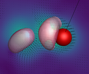
  $m^*$ values. One could certainly use different vortex identification criteria since a proper selection of the threshold leads to similar representations independent of the chosen criterion (Chakraborty, Balachandar & Adrian Reference Chakraborty, Balachandar and Adrian2005). The obtained iso-surface images were imported and further processed in Wolfram Mathematica 12. First, each image was applied a semantic segmentation based on threshold binarisation and a colour negation. This led to the construction of images of ‘zeros’ (white) and ‘ones’ (black) depending on the pixel intensity. Furthermore, a bounding box was computed for connected regions counting more than 2000 pixels. This procedure results in the elimination of all objects other than large coherent iso-surfaces. The vortex trajectories were derived from the bounding box coordinates. Thus including the temporal information based on the recording frequency allowed for further analysis of the vortex propagation velocities. Figure 2(a) displays an application of the DOT showing two equally sized vortices and their corresponding bounding boxes, as well as the trajectories from the previous time steps. The plotted trajectories describe the separation and downward motion of the red highlighted vortex ring, while the black one stays on the circular path.

Figure 2. (a) Example image of vortex tracking showing two equally sized vortices and their corresponding bounding boxes, as well as the trajectories from the previous time steps. (b) Iso-surface values for visualisation of vortical structures based on the period of the first oscillation.
3. Results
3.1. Oscillation frequency and amplitude decay
Table 2 summarises the measured periods of the first oscillation cycle  $T$ and amplitude peaks $\theta _{max}$ obtained from the recordings. The period decreases nonlinearly with increasing mass ratios $m^*$, while the peak angular displacement at the end of the first swing grows logarithmically with $m^*$. Normalising the oscillation frequency $f=1/T$ with the natural pendulum frequency $f_{n}=(1/2{\rm \pi} )\sqrt {g/L}$ gives $f^*$. In figure 3(a), this normalised frequency $f^*$ is shown for the spheres and the heavy cylinder pendulums from Mathai et al. (Reference Mathai, Loeffen, Chan and Wildeman2019). For both spheres and cylinders, the deviation between natural frequency and measured frequency increases significantly with decreasing $m^*$. They follow the same trend, having a steep gradient for $m^* <2.5$. For denser materials, $f^*$ of sphere and cylinder are very similar, while for $m^* <2$, differences are present.
Table 2. Mass ratio  $m^*$, period of the first oscillation cycle $T$, maximum angular position at the end of the first swing $\theta _{max}$.


Figure 3. The present experiments of heavy spherical pendulums with  $m^*\in [1.14, 14.95]$ are plotted as filled black diamonds, while the experimental data of heavy cylindrical pendulums by Mathai et al. (Reference Mathai, Loeffen, Chan and Wildeman2019) are plotted as purple squares. (a) Normalised oscillation frequency $f^*=f/f_n$ for different $m^*$. (b) Amplitude envelope $\theta _{\tau _{ref}}$ against normalised oscillation frequency $f^*$ after a time $\tau _{ref}=3{\rm \pi} \sqrt {L/g}$.
By fitting an envelope to the amplitude peaks over time, we determined the amplitude envelope  $\theta _{\tau _{ref}}$ at the reference time $\tau _{ref}=3{\rm \pi} \sqrt {L/g}$. Plotting $\theta _{\tau _{ref}}$ against $f^*$ in figure 3(b), optimal damping is found at $f^*\approx 0.7$. This corresponds to $m^*\approx 2.5$. In comparison, Mathai et al. (Reference Mathai, Loeffen, Chan and Wildeman2019) present a damping optimum at $m^*\approx 2$ for heavy cylinders. These novel findings can have important practical consequences to improve the naval stability of crane vessels.
Interestingly, the damping of the sphere shows a more distinct non-monotonic dependence on  $m^*$. According to Mathai et al. (Reference Mathai, Loeffen, Chan and Wildeman2019), the non-monotonic damping is an effect of the nonlinear drag, implying that this effect is more significant for spherical pendulums. Additionally, the different added mass values of the cylinder and the sphere may impact the different mass damping ratios. Considering the different initial deflection angles (90 $^\circ$ in Mathai et al. (Reference Mathai, Loeffen, Chan and Wildeman2019) versus 37.5 $^\circ$ in the present study), the amplitude of the spherical pendulum decays much more slowly than the less streamlined cylinder. This is partially explained by the drag coefficient $C_D$, which is generally lower for spheres than for cylinders for $Re>10$. Further, the influence of $Re$ on $C_D$ is different for spheres and cylinders in the present range of $Re$ (Hoerner Reference Hoerner1965). This effects the nonlinear growth of the drag in proportion to the square of the velocity. Still, there are other phenomena that are affecting the fluid drag related to vortex shedding (Williamson & Govardhan Reference Williamson and Govardhan1997; Mathai et al. Reference Mathai, Loeffen, Chan and Wildeman2019). To better account for the drag oscillations caused by vortex-induced vibrations, knowledge regarding the vortex shedding topology is a requirement (Williamson & Govardhan Reference Williamson and Govardhan1997). The following subsections are dedicated to better understanding the vortex dynamics of oscillating systems in a dense fluid.
3.2. Vortex dynamics
For all  $m^*$ ratios, the motion of the sphere induced a toroidal vortex structure that formed at the initial phase of the first downward swing (figure 4a). For all $m^*$, the observed toruses had initial diameter ( $D_{vor}$) approximately $2D$ when the iso-surface threshold was selected as described in § 2.3. However, at some point, the vertical structures begin to separate into two clearly distinguishable equally sized vortex rings, as shown in figures 4(b–d). This separation process and downward shedding were present in all experimental observations. Soon after its formation, the vortex ring propagates on a nearly linear path towards the bottom (figure 6). This downward propagation of the vortex is explained by the momentum imparted from the motion of the pendulum bob (Worf et al. Reference Worf, Khosronejad, Gold, Reiterer, Habersack and Sindelar2022). While propagating, the vortex ring remains remarkably stable until reaching its terminal velocity and eventually dissipating. This behaviour is similar to the aforementioned case of the cylinder pendulum investigated experimentally by Mathai et al. (Reference Mathai, Loeffen, Chan and Wildeman2019) and numerically by Worf et al. (Reference Worf, Khosronejad, Gold, Reiterer, Habersack and Sindelar2022). Based on their findings, Worf et al. (Reference Worf, Khosronejad, Gold, Reiterer, Habersack and Sindelar2022) described the development and downward shedding of the vortex ring in the wake of a cylinder during the first swing. Later on, the vortex stretches out and dissipates near the side walls of the glass tank. For comparable radii, although only 2-D, the numerical results from Mongelli & Battista (Reference Mongelli and Battista2020) also show vortex shedding dominated by vertical downward-moving vortices. In our experimental observations, the overall process stays the same for all ratios $m^*$, but the instant at which the first vortex is shed clearly differs. The beginning of the shedding ( $t_{vs}$) was determined by the above-mentioned DOT procedure, and the image frame where the trajectory of the downward-moving vortex leaves the circular pendulum path was selected. More specifically, herein, it was the instant for which the vertical distance $d_y$ ( $y$-direction in figures 2 and 4) between the trajectories $d_y \geq D/4$ was selected. As expected, the time for the formation and detachment of the vortex decreases as the mass ratios increase. However, for $m^* \geq 6$, the vortex separation time decreases slightly. Hence the relation between $t_{vs}$ and $m^*$ could be described by a power law, as shown in figure 5(a). In addition, the obtained values of $t_{vs}$ are compared with the theoretical shedding frequency based on the Strouhal number $S_r$ (Strouhal Reference Strouhal1878). From $S_r=f_{vs}D/v_p$, the vortex shedding frequency ( $\,f_{vs}$) can be derived. The time $t_{vs}$ when the first vortex ring is shed can be estimated based on $f_{vs}$:
 \begin{equation} t_{vs}=\frac{1}{f_{vs}}=\frac{D}{S_rv_p}, \end{equation}
where  $D$ is the characteristic length represented by the sphere diameter, and $v_p$ is the relative pendulum velocity. The mean velocity $v_p=\theta _0 L / t_p$ is derived from the time $t_p$ that the sphere takes to swing from $\theta _0 =37.5^\circ$ to the perigee $\theta _p=0^\circ$. With the Strouhal number $S_r = 0.21$ (for $Re\in [4\times 10^2,1\times 10^4]$), the time $t_{vs}$ is estimated. This calculated shedding time $t_{vs}$ and the experimental results plotted in figure 5(a) suggest a high level of agreement for all $m^*$ ratios.

Figure 4. Shedding topology during the first downward swing for  $m^* = 6.0$ after (a) $t=0.146$ s, (b) $t=0.178$ s, (c) $t=0.210~$s, and (d) $t=0.242$ s.

Figure 5. (a) Instant of time when the first vortex is shed as a function of  $m^*$. Comparison of the instant of first vortex shedding $t_{vs}$ obtained from the present experimental observations and theoretical approach based on the Strouhal number $S_r$. (b) Non-dimensional propagation velocity $U^*_{vor}$ of the downward moving vortex ring.
3.3. Vorticity transport
Figure 5(b) shows the non-dimensional velocity evolution  $U^*_{vor}=U_{vor}/\sqrt {gL}$ of the first detached vortex for various $m^*$. Starting at $t_{vs}$, the vortex velocity $U_{vor}$ is derived from the distance covered by the DOT bounding box centres between two frames, divided by the corresponding time increments. As seen, for $m^*>1.41$, $U^*_{vor}$ undergoes a quick decay. Initially, $U^*_{vor}$ is in the range between 0.06 and 0.40, with higher velocities related to higher mass ratios. In contrast, the terminal velocity at which the vortex dissipates seems to be independent of $m^*$. In addition, for $m^*>1.41$, another vortex is shed at the turning point of the pendulum. This was also observed by Bolster et al. (Reference Bolster, Hershberger and Donnelly2010) for sufficiently large amplitudes. A video showing the vortex shedding for $m^*=3.26$ can be found in supplementary movie 1, available at https://doi.org/10.1017/jfm.2023.170. Figures 6(a–c) show the time-averaged $z$ vorticity $\omega _z$ normalised by $\omega _{zmax}$ for three different mass ratios $m^*=2.50,3.26,6.00$. Red represents positive values of $\omega _z$, whereas blue indicates a negative $z$ vorticity. The time averaging was conducted for the duration of time until the first turning point was reached. Since the main topological features are the two equally sized vortex rings, the time-averaged results produce a bifurcating vortex tube. During the separation process, the sphere detaches from the upper clockwise rotating part of the shed vortex, and fluid is lifted up in the wake of the sphere during the closure of the shed vortex. This can be seen for $m^*=3.26$ in a video animation provided in supplementary movie 2. The new insights into the interaction of the sphere's wake and the detaching vortex can be useful especially to improve both numerical and analytical models. For example, Mathai et al. (Reference Mathai, Loeffen, Chan and Wildeman2019) presents a wake correction for a cylindrical pendulum that starts at the first turning point of the pendulum when the cylinder enters the disturbed flow field. However, the numerical re-investigation of Worf et al. (Reference Worf, Khosronejad, Gold, Reiterer, Habersack and Sindelar2022) suggests an earlier start of the wake correction some time before the first turning point. This is supported by the present observations as the sphere certainly interacts with its own wake during the vortex separation process. At least for the spherical pendulum, a possible start of the wake correction model during the first downward swing is indicated.

Figure 6. Time-averaged vorticity data for three different mass ratios  $m^*=2.50,3.26,6.00$. (a–c) Iso-surfaces representing the 0.25 value of the maximum-normalised vorticity magnitude coloured by the normalised $z$ vorticity $\omega _z$. (d–f) Middle slices of the corresponding vorticity magnitude $|\omega |/\omega _{max}$.
Figures 6(d–f) mark the corresponding middle  $z$ slices of the maximum-normalised vorticity magnitude $|\omega |/\omega _{max}$. It can be seen clearly that the highest time-averaged values are present not in the pendulum's direct wake but in the detached vortex's downward path. Also, figures 6(d–f) suggest that the angle at which the vortex propagates downwards is independent of $m^*$. To provide evidence, a linear regression is performed on the trajectories of the shed vortices from the DOT method. The resulting propagation angle $\phi$ is measured between the $x$-axis (bottom of the tank) and the path of the detached vortex in clockwise direction. Table 3 lists $\phi$ divided by $\theta _0$ and the corresponding coefficients of determination $R^2$. The direction of vortex propagation is approximately orthogonal to the pendulum rod at $\theta _0$ for the observed $m^*$ values. More specifically, $\phi$ varies between 36 $^\circ$ and 41 $^\circ$, showing no significant dependency on $m^*$. Notably, the mass independence of $\phi$ contrasts with the correlation of $t_{vs}$ and $U^*_{vor}$ with $m^*$.
Table 3. Angle of vortex propagation  $\phi$ in relation to the initial deflection $\theta _0$ for different $m^*$. The values of $\phi$ and the corresponding coefficients of determination $R^2$ are derived from linear regression of the vortex trajectories from DOT.

4. Conclusions
Within this work, a detailed analysis concerning the fluid–structure interaction of heavy spherical pendulums oscillating in water is presented for a wide range of  $m^*$. Special emphasis was placed on the characterisation of the vortex shedding topology. Based on rigorous tr-3-D-PTV measurements and a novel digital object tracking (DOT) method, the topology of vortical flow structures arising from the 3-D nonlinear interaction of water and the spherical pendulum was investigated. By combining the spatial and temporal signatures of the present vortex structures, the novel DOT method allowed for a more detailed analysis of vorticity iso-surface plots, including vortex trajectories and propagation velocities. The introduced DOT approach to treat iso-surface representations as distinct digital objects and track them potentially advances future research on various highly relevant topics like vortex shedding topology, vortex dynamics and vortex-induced vibrations.
This study revealed a characteristic vortex shedding topology during the first downward swing of underwater pendulums for the full range of  $m^*$ and a constant initial deflection angle $\theta _0 = 37.5^{\circ }$. Our observations showed that first, a toroidal vortex is formed in the wake of the spherical pendulum, which splits up into two separate structures of equal size. One vortex remains on the pendulum's circular path, and the other detaches. The shed vortex ring propagates on a nearly linear path downwards, where the angle of propagation is independent of $m^*$ and approximately orthogonal to the initial angle of deflection $\theta _0$. For all $m^*$, an analogy of the vortex ring dimensions ( $D_{vor} \sim 2D$) is found when scaling the vorticity with the pendulum period ( $T$). The theoretical vortex shedding time scale based on the Strouhal number proved to agree reasonably with the experimentally determined time of vortex shedding using our DOT approach, suggesting it to be a reliable predictor for the onset of vortex shedding. While the time of separation and the initial speed of the vortical structure depended on the mass ratio $m^*$, the terminal velocities are independent of $m^*$.
Based on the oscillation period and the amplitude envelope, we found evidence of a non-monotonic relation between amplitude decay and  $m^*$. A damping optimum is present when $m^*\approx 2.5$. The results on mass-dependent structural damping and complex vortex dynamics can be beneficial for the enhancement of maritime infrastructure, underwater mining operations, and naval stability of crane vessels. Further, this highlights the importance of knowing the underlying mechanisms like added mass, (nonlinear) drag and vortex dynamics to better understand the interaction between fluid and structures, not only for the pendulum in a dense fluid. Eventually, the attractiveness of the humble pendulum to address fundamental questions in fluid dynamic research is pointed out once again.
Supplementary material
Supplementary movies are available at https://doi.org/10.1017/jfm.2023.170.
Acknowledgements
T.G. thanks N. Kaiblinger for his input on digital object tracking.
Funding
This research was funded by the Austrian Science Fund (FWF, P33493-N), the Christian Doppler Research Association, and the Austrian Federal Ministry for Digital and Economic Affairs and the National Foundation of Research, Technology, and Development of Austria (T.G., K.R., D.W.).
Declaration of interests
The authors report no conflict of interest.
Data availability statement
The datasets analysed during the current study can be made available by the corresponding author on reasonable request.


 Open access