


1. Introduction
The flow of gravity currents became a classic research topic during the past three decades (e.g. Huppert & Woods Reference Huppert and Woods1995; Acton, Huppert & Worster Reference Acton, Huppert and Worster2001; Pritchard, Woods & Hogg Reference Pritchard, Woods and Hogg2001; Neufeld, Vella & Huppert Reference Neufeld, Vella and Huppert2009; Linden Reference Linden2012; Pegler, Huppert & Neufeld Reference Pegler, Huppert and Neufeld2014; Zheng et al. Reference Zheng, Guo, Christov, Celia and Stone2015a; Hinton & Woods Reference Hinton and Woods2018). In addition to its occurrence in nature during magma spreading, groundwater motion and grounding line movement (e.g. Huppert Reference Huppert1982; Kochina, Mikhailov & Filinov Reference Kochina, Mikhailov and Filinov1983; Kowal & Worster Reference Kowal and Worster2015, Reference Kowal and Worster2020), there are also important practical applications such as drainage and irrigation in soils and sands (e.g. Boussinesq Reference Boussinesq1904; Bear Reference Bear1972; Acton et al. Reference Acton, Huppert and Worster2001; Pritchard et al. Reference Pritchard, Woods and Hogg2001; Zheng et al. Reference Zheng, Soh, Huppert and Stone2013; Liu, Zheng & Stone Reference Liu, Zheng and Stone2017; Yu, Zheng & Stone Reference Yu, Zheng and Stone2017), recovery of fluid-phase resources from porous rocks (Woods & Mason Reference Woods and Mason2000; Zheng & Neufeld Reference Zheng and Neufeld2019; Nijjer, Hewitt & Neufeld Reference Nijjer, Hewitt and Neufeld2022), disposal of chemicals and waste water in aquifers (e.g. Huppert & Woods Reference Huppert and Woods1995; Hinton & Woods Reference Hinton and Woods2019; Bhamidipati & Woods Reference Bhamidipati and Woods2020), seasonal thermal energy storage (e.g. Dudfield & Woods Reference Dudfield and Woods2012), transport of gas and liquids in channels and pipes (e.g. Hallez & Magnaudet Reference Hallez and Magnaudet2009; Taghavi et al. Reference Taghavi, Seon, Martinez and Frigaard2009; Zheng, Rongy & Stone Reference Zheng, Rongy and Stone2015b; Horsley & Woods Reference Horsley and Woods2017), and geological sequestration of  ${\rm CO}_2$ (e.g. Lyle et al. Reference Lyle, Huppert, Hallworth, Bickle and Chadwick2005; Nordbotten & Celia Reference Nordbotten and Celia2006; Hesse, Orr & Tchelepi Reference Hesse, Orr and Tchelepi2008; Farcas & Woods Reference Farcas and Woods2009; Neufeld et al. Reference Neufeld, Vella and Huppert2009; MacMinn, Szulczewski & Juanes Reference MacMinn, Szulczewski and Juanes2010; MacMinn & Juanes Reference MacMinn and Juanes2013; Guo et al. Reference Guo, Zheng, Celia and Stone2016; Zheng & Neufeld Reference Zheng and Neufeld2019; Nijjer et al. Reference Nijjer, Hewitt and Neufeld2022). Gravity currents also appear in ocean and the atmosphere such as the propagation of ocean currents along the sea floor and the generation of turbidity currents and sand storms, in which case the flow can become turbulent and the influence of entrainment and mixing can become important (e.g. Rottman & Simpson Reference Rottman and Simpson1983; Thomas, Marino & Linden Reference Thomas, Marino and Linden1998; Marino, Thomas & Linden Reference Marino, Thomas and Linden2005; Linden Reference Linden2012; Sher & Woods Reference Sher and Woods2015). A recent review is also available with a focus on the influence of boundaries, including leakage, flow confinement, and converging and deformable boundaries (Zheng & Stone Reference Zheng and Stone2022).
While there are many previous studies on the fundamentals of single gravity current flows, partly inspired by the aforementioned applications in either unconfined or confined porous rocks, the interaction of multiple gravity currents has not been thoroughly investigated despite its practical relevance, which is the focus of the current study. We are aware of an earlier work (Woods & Mason Reference Woods and Mason2000), where the dynamic interaction of two unconfined gravity currents in an infinitely deep porous medium was studied, in which case the ambient fluid is effectively quiescent and the nature of spreading is nonlinear diffusive for both currents (e.g. Pattle Reference Pattle1959; Gratton & Minotti Reference Gratton and Minotti1990; Huppert & Woods Reference Huppert and Woods1995). Their laboratory experiments in a Hele-Shaw cell also demonstrate that fluid mixing is negligible during the interaction of viscous currents, and the interfaces between the injecting and displaced fluids remain sharp within the time and length scales of interest. We are also made aware of another work on the interaction of two viscous gravity currents into a liquid ocean, which was inspired to describe the formation of grounding zone wedges of marine ice sheets and shelves (Kowal & Worster Reference Kowal and Worster2020). Their experiments, using glycerine, golden syrup and salt solution as mimicking fluids, also show that fluid mixing is negligible for the parameter range considered, and the fluid–fluid interfaces remain sharp during the time evolution.
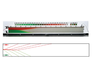
Natural porous rocks are typically layered with significant permeability and porosity variations between neighbouring layers (e.g. Phillips Reference Phillips1991; Dullien Reference Dullien1992; Huppert & Woods Reference Huppert and Woods1995). Therefore, it is also important to study gravity current flows in confined porous spaces of finite depth, and indeed there is a long list of previous reports on many important and interesting facets of confined currents (e.g. Huppert & Woods Reference Huppert and Woods1995; Nordbotten & Celia Reference Nordbotten and Celia2006; Gunn & Woods Reference Gunn and Woods2011; Pegler et al. Reference Pegler, Huppert and Neufeld2014; Zheng et al. Reference Zheng, Guo, Christov, Celia and Stone2015a; Guo et al. Reference Guo, Zheng, Celia and Stone2016; Hinton & Woods Reference Hinton and Woods2018). In this paper, we are motivated to study the dynamic interaction of two confined gravity currents, one heavier and one lighter, injected simultaneously into a porous layer of finite depth, as shown in figure 1. Such flows are relevant to the applications of enhanced oil recovery, geological  ${\rm CO}_2$ sequestration and cleaning of confined porous spaces.

Figure 1. Dynamic interaction of two gravity currents in an infinitely long porous layer of finite thickness  $h_0$, initially filled with another ambient fluid. The permeability and porosity of the porous layer are denoted by $k$ and $\phi$, respectively, and the viscosity and density of the fluids are denoted by $\mu _i$ and $\rho _i$ within layer $i=\{1,2,3\}$. The pressure and velocity fields are denoted by $p_i$ and $u_i$, respectively. It is assumed that $\rho _1 > \rho _2 > \rho _3$, such that a heavier gravity current is generated along the base, while a lighter gravity current is generated along the top. The profile shapes are denoted by $h_1(x,t)$ and $h_2(x,t)$ (or $\hat h_2 \equiv h_0-h_2$, equivalently), and the frontal locations are denoted by $x_{f1}(t)$ and $x_{f2}(t)$. The location where three fluids meet is denoted by $(x_*,h_*)$. The area injection rates of the heavier and lighter currents are denoted by $q_1$ and $q_2$.
As the currents approach each other in a confined space (due to injection) and start to interact at late times (figure 1b), the motion of the ambient fluid has to be considered due to the creation of a background pressure gradient along the cap rock, which is fundamentally different from the interaction of unconfined currents (Woods & Mason Reference Woods and Mason2000). Most importantly, the viscosity contrast between the injecting and displaced fluids becomes an important factor that can significantly impact the outcome of the flow (e.g. Zheng et al. Reference Zheng, Guo, Christov, Celia and Stone2015a). Correspondingly, the nature of gravity current spreading becomes nonlinear advective-diffusive in confined porous layers, as the flow is driven by both the buoyancy and pumping (injection) forces and the interplay of each driving force can vary significantly with time and space (e.g. Huppert & Woods Reference Huppert and Woods1995; Pegler et al. Reference Pegler, Huppert and Neufeld2014; Zheng et al. Reference Zheng, Guo, Christov, Celia and Stone2015a). The interaction of confined gravity currents hence becomes more complicated, as we show in this paper. In particular, eight different regimes of dynamic interaction arise eventually, as controlled by four dimensionless parameters with regards to the viscosity ratio, buoyancy contrast and the partition of injection rates of the injecting fluids. In particular, in four of the eight regimes (regimes 2, 6–8), self-similar solutions can be constructed by combining appropriately the three basic solutions of shock, rarefaction and travelling-wave solutions identified for single current injection (e.g. Huppert & Woods Reference Huppert and Woods1995; Pegler et al. Reference Pegler, Huppert and Neufeld2014; Zheng et al. Reference Zheng, Guo, Christov, Celia and Stone2015a). In the other four regimes (regimes 1, 3–5), new basic flow patterns appear and the self-similar interface shape is described by logarithm and error functions.
This paper is structured as follows. In § 2, we first present a theoretical model of two coupled partial differential equations (PDEs) to describe the profile shape evolution of the interacting gravity currents. Four dimensionless parameters are identified that distinguish the flow into eight different regimes of dynamic interaction at late times. In § 3, we discuss in detail the asymptotic behaviours of the eight different regimes of dynamic currents interaction. We obtain asymptotic solutions in all eight regimes based on different similarity and travelling-wave transforms. We also briefly remark on the time transition from early-time unconfined currents to late-time interacting currents in confined porous layers. Before we close the paper in § 4, potential implications in  ${\rm CO}_2$-water co-flooding projects in oil fields are also addressed briefly, employing geophysical and operational parameters in practical projects.
2. Theoretical model
2.1. Governing equations
We study the dynamic interaction of heavier and lighter gravity currents in a confined porous layer in a Cartesian configuration, as shown in figure 1. We follow and extend the standard steps to study the dynamics of single gravity current injection into a confined porous layer (e.g. Huppert & Woods Reference Huppert and Woods1995; Pegler et al. Reference Pegler, Huppert and Neufeld2014; Zheng et al. Reference Zheng, Guo, Christov, Celia and Stone2015a) and the interaction of two unconfined gravity currents (e.g. Woods & Mason Reference Woods and Mason2000). In the model problem, fluids 1 and 3 are both injected into a homogeneous porous layer with finite thickness  $h_0$, initially filled with ambient fluid 2. The density and viscosity of the fluids are denoted by $\rho _i$ and $\mu _i$, respectively, with $i = \{1,2,3\}$, and the permeability and porosity of the porous layer are denoted by $k$ and $\phi$. It is assumed that $\rho _1 > \rho _2 > \rho _3$ in the current work, such that two gravity currents are generated, including a lighter one that spreads along the top ( $\kern0.7pt y=h_0$) and a heavier one that spreads along the base ( $\kern0.7pt y=0$). We neglect the influence of fluids mixing and wetting and capillary forces such that sharp interfaces are maintained between different fluids. The profile shape of the heavier current is denoted by $h_1 (x,t)$ and that of the lighter one is denoted by $h_2 (x,t)$, or $\hat {h}_2 (x,t) \equiv h_0 - h_2 (x,t)$, equivalently. Meanwhile, the thickness of the displaced (ambient) layer can also be estimated by $h_2 (x,t) - h_1 (x,t) = h_0 - h_1(x,t) - \hat {h}_2 (x,t)$.
It is also assumed that the fluid–fluid interfaces are long and thin, such that the vertical component of the Darcy velocity is small compared with the horizontal component. This is seen directly from the continuity equation for incompressible flow  $\partial u/\partial x + \partial v/\partial y = 0$, i.e. the characteristic velocity and length scales in horizontal and vertical directions must satisfy $u_c/x_c \sim v_c/y_c$. We can hence define an aspect ratio $\delta \equiv y_c/x_c$ of a gravity current, such that $v_c/u_c \sim \delta$. We must need $\delta \ll 1$ for the vertical velocity scale to be negligible, i.e. $v_c \ll u_c$. Accordingly, the fluid pressure follows hydro-static distribution within each layer and is given by
 \begin{gather} p_1 (x,y,t) = p_0 (x,t) - \rho_1 g y, \quad 0 \leq y \leq h_1, \end{gather}
 \begin{gather}p_2 (x,y,t) = p_0 (x,t) - \rho_1 g h_1 - \rho_2 g(y-h_1), \quad h_1 < y \leq h_2, \end{gather}
 \begin{gather}p_3 (x,y,t) = p_0 (x,t) - \rho_1 g h_1 - \rho_2 g(h_2-h_1) - \rho_3 g(y-h_2), \quad h_2 < y \leq h_0, \end{gather}
where  $p_i(x,y,t)$ denotes the pressure field within fluid layer $i = \{1,2,3\}$ and $p_0 (x,t)$ denotes the background pressure distribution along the base of the porous layer ( $\kern0.7pt y=0$). Here, $g$ is gravitational acceleration. The horizontal pressure gradients that drive the flow can then be calculated as
 \begin{gather} \frac{\partial p_1}{\partial x} = \frac{\partial p_0}{\partial x}, \end{gather}
 \begin{gather}\frac{\partial p_2}{\partial x} = \frac{\partial p_0}{\partial x} - {\rm \Delta} \rho_1 g \frac{\partial h_1}{\partial x}, \end{gather}
 \begin{gather}\frac{\partial p_3}{\partial x} = \frac{\partial p_0}{\partial x} - {\rm \Delta} \rho_1 g \frac{\partial h_1}{\partial x} - {\rm \Delta} \rho_2 g\frac{\partial h_2}{\partial x}, \end{gather}
where  ${\rm \Delta} \rho _1 \equiv \rho _1 -\rho _2 > 0$ and ${\rm \Delta} \rho _2 \equiv \rho _2 -\rho _3 > 0$. Darcy's Law can now be applied to provide the horizontal velocity of the fluids within each layer
 \begin{gather} u_1 ={-}\frac{k}{\mu_1} \frac{\partial p_1}{\partial x} ={-}\frac{k}{\mu_1} \frac{\partial p_0}{\partial x}, \end{gather}
 \begin{gather}u_2 ={-}\frac{k}{\mu_2} \frac{\partial p_2}{\partial x} ={-}\frac{k}{\mu_2} \left( \frac{\partial p_0}{\partial x} - {\rm \Delta} \rho_1 g \frac{\partial h_1}{\partial x} \right), \end{gather}
 \begin{gather}u_3 ={-}\frac{k}{\mu_3} \frac{\partial p_3}{\partial x} ={-}\frac{k}{\mu_3} \left( \frac{\partial p_0}{\partial x} - {\rm \Delta} \rho_1 g \frac{\partial h_1}{\partial x} - {\rm \Delta} \rho_2 g\frac{\partial h_2}{\partial x} \right). \end{gather}
It is already seen that, physically, a horizontal velocity for the fluid layers can be driven by both the background pressure gradient ( $\partial p_0/\partial x$) and buoyancy ( $\propto \partial h_1/\partial x$ or $\propto \partial h_2/\partial x$). We later show that $\partial p_0/\partial x$ is also under the influence of injection rate, in addition to the buoyancy of the injected fluids. It is also of interest to note that, based on (2.2), the pressure gradient $\partial p_i/\partial x$ within each fluid layer is independent of $y$. Accordingly, within the same fluid layer, at any time $t$ of interest, the Darcy velocity remains the same along the $y$ direction at the same horizontal position $x$.
$x$.
In addition, local conservation of fluid volume (i.e. local continuity) in  $[x, x + {\rm d} x]$ within each fluid layer requires that
 \begin{gather} \phi \frac{\partial h_1}{\partial t} + \frac{\partial (h_1 u_1)}{\partial x} = 0, \end{gather}
 \begin{gather}\phi \frac{\partial (h_2 - h_1)}{\partial t} + \frac{\partial [(h_2 - h_1) u_2]}{\partial x} =0, \end{gather}
 \begin{gather}\phi \frac{\partial (h_0 - h_2)}{\partial t} + \frac{\partial [(h_0 - h_2) u_3]}{\partial x} =0. \end{gather}
Physically, this says that the shape evolution of a fluid layer is dependent on the net fluxes across the vertical boundaries of an infinitely thin control volume  $[x, x + {\rm d} x]$. Then, by substituting (2.3a,c) into (2.4a,c), we arrive at the evolution equations for the interface shape of the heavier current $h_1 (x,t)$ and the lighter current $\hat {h}_2 (x,t) \equiv h_0 - h_2 (x,t)$:
 \begin{gather} \phi \frac{\partial h_1}{\partial t} - \frac{k}{\mu_1} \frac{\partial}{\partial x} \left( h_1 \frac{\partial p_0}{\partial x} \right) = 0, \end{gather}
 \begin{gather}\phi \frac{\partial \hat{h}_2}{\partial t} - \frac{k}{\mu_3} \frac{\partial}{\partial x} \left[ \hat{h}_2 \left( \frac{\partial p_0}{\partial x} - {\rm \Delta} \rho_1 g \frac{\partial h_1}{\partial x} + {\rm \Delta} \rho_2 g \frac{\partial \hat{h}_2}{\partial x} \right) \right] = 0, \end{gather}
including a background pressure gradient  $\partial p_0 / \partial x$ along the base of the porous layer ( $\kern0.7pt y=0$) that is yet to be determined.
Global conservation of the total volume of the injected fluids, meanwhile, provides that
 \begin{gather} \phi \int_0^{x_{f1}(t)} h_1 (x,t) \,\mathrm{d} x = q_1 t, \end{gather}
 \begin{gather}\phi \int_0^{x_{f2}(t)} \hat{h}_2 (x,t) \,\mathrm{d} x = q_2 t, \end{gather}
with  $q_1$ and $q_2$ representing the area injection rates, and $x_{f1}(t)$ and $x_{f2}(t)$ representing the time-dependent locations of the propagating front of the heavier and lighter currents, respectively. The form of (2.6) indicates that the injection of the heavier and lighter fluids proceeds simultaneously at constant rates $q_1$ and $q_2$. However, we also note that the analysis can be extended to account for the influence of time-dependent injection rates.
Then, denoting the total injection rate as  $q \equiv q_1+q_2$, equivalently, volume conservation requires that
 \begin{equation} q = h_1 u_1 + (h_0-h_1-\hat{h}_2) u_2 + \hat{h}_2 u_3, \end{equation}
considering the contribution of all three fluid layers. Then, by substituting (2.3a–c) into (2.7), we obtain an explicit expression for the background pressure gradient in terms of  $h_1 (x,t)$ and $\hat {h}_2 (x,t)$ as
 \begin{equation} \frac{\partial p_0}{\partial x} = \frac{-\dfrac{\mu_1}{k} q + {\rm \Delta} \rho_1 g [ M_2(h_0-h_1-\hat{h}_2) + M_3\hat{h}_2] \dfrac{\partial h_1}{\partial x}- {\rm \Delta} \rho_2 g M_3 \hat{h}_2 \dfrac{\partial \hat{h}_2}{\partial x}}{h_1 + M_2 (h_0-h_1-\hat{h}_2) + M_3 \hat{h}_2}, \end{equation}
where two viscosity ratios  $M_2$ and $M_3$ have been introduced as
 \begin{equation} M_2 \equiv \frac{\mu_1}{\mu_2}\quad \mbox{and}\quad M_3 \equiv \frac{\mu_1}{\mu_3}. \end{equation}
Equation (2.8) indicates that there are three major contributions of the background pressure gradient  $\partial p_0/\partial x$ and hence the flow: the pumping force ( $\propto q$), the buoyancy force of the heavier current ( $\propto {\rm \Delta} \rho _1 g$) and the buoyancy force of the lighter current ( $\propto {\rm \Delta} \rho _2 g$). Meanwhile, (2.8) is ready to be substituted back into (2.5) to provide two coupled PDEs for the time evolution of the profile shape of the heavier and lighter currents $h_1 (x,t)$ and $\hat {h}_2 (x,t)$:
 \begin{gather} \phi \frac{\partial h_1}{\partial t} \!+\! \frac{\partial}{\partial x} \left[ \frac{q h_1 \!-\! \dfrac{{\rm \Delta} \rho_1 g k}{\mu_1}[ M_2(h_0-h_1-\hat{h}_2)+M_3\hat{h}_2]h_1\dfrac{\partial h_1}{\partial x} + \dfrac{{\rm \Delta} \rho_2 g k}{\mu_3} h_1 \hat h_2 \dfrac{\partial \hat{h}_2}{\partial x} }{h_1+M_2(h_0-h_1-\hat{h}_2)+M_3\hat{h}_2} \right] \!=\! 0, \end{gather}
 \begin{gather}\phi \frac{\partial \hat{h}_2}{\partial t} \!+\! \frac{\partial}{\partial x} \left[ \frac{M_3 q \hat h_2 + \dfrac{{\rm \Delta} \rho_1 g k}{\mu_1}M_3 h_1\hat h_2 \dfrac{\partial h_1}{\partial x} \!-\! \dfrac{{\rm \Delta} \rho_2 g k}{\mu_3}[ M_2(h_0-h_1\!-\!\hat{h}_2)\!+\!h_1]\hat h_2\dfrac{\partial \hat{h}_2}{\partial x}}{h_1\!+\!M_2(h_0\!-h_1\!-\hat{h}_2)\!+\!M_3\hat{h}_2} \right] \!=\! 0. \end{gather}
Similarly, (2.10a,b) indicate that, physically, the time evolution of the profile shape of the two currents is under the influence of the pumping force ( $\propto q$), the buoyancy force of the heavier current ( $\propto {\rm \Delta} \rho _1 g$) and the buoyancy force of the lighter current ( $\propto {\rm \Delta} \rho _2 g$). The competition between each of them can possibly vary with space and time, and leads to many facets of dynamic behaviours of the interacting gravity currents.
Finally, to complete the problem, appropriate initial and boundary conditions (IBCs) are needed. In particular, we assume that, initially, there is only the ambient fluid 2 filling up the entire space of the porous layer, which provides a set of initial conditions:
 \begin{equation} h_1 (x,0) = 0\quad \mbox{and}\quad \hat{h}_2 (x,0) = 0. \end{equation}
In addition, the frontal condition of viscous gravity currents leads to a set of Dirichlet boundary conditions at  $x=x_{f1}(t)$ and $x=x_{f2}(t)$:
 \begin{equation} h_1 (x_{f1}(t),t) = 0\quad \mbox{and}\quad \hat{h}_2 (x_{f2}(t),t) = 0. \end{equation}
By integrating the evolution equations (2.10a,b) from  $x=0$ towards $x = \infty$ and applying the global conservation of fluid volume (2.6a,b), we obtain a set of flux boundary conditions at $x = 0$:
 \begin{gather} \left.\frac{q h_1 - \dfrac{{\rm \Delta} \rho_1 g k}{\mu_1}[ M_2(h_0-h_1-\hat{h}_2)+M_3\hat{h}_2]h_1\dfrac{\partial h_1}{\partial x} + \dfrac{{\rm \Delta} \rho_2 g k}{\mu_3} h_1 \hat h_2 \dfrac{\partial \hat{h}_2}{\partial x} }{h_1+M_2(h_0-h_1-\hat{h}_2)+M_3\hat{h}_2} \right|_{x=0} = q_1, \end{gather}
 \begin{gather}\left.\frac{M_3 q \hat h_2 + \dfrac{{\rm \Delta} \rho_1 g k}{\mu_1} M_3 h_1\hat h_2 \dfrac{\partial h_1}{\partial x} - \dfrac{{\rm \Delta} \rho_2 g k}{\mu_3}[ M_2(h_0-h_1-\hat{h}_2)+h_1]\hat h_2\dfrac{\partial \hat{h}_2}{\partial x}}{h_1+M_2(h_0-h_1-\hat{h}_2)+M_3\hat{h}_2} \right|_{x=0} = q_2. \end{gather}
 It is important to note that to arrive at the flux conditions (2.13a,b), we have also assumed that there is no entrainment of the ambient fluid into the gravity currents at the location of the propagating fronts  $x_{f1}(t)$ and $x_{f2}(t)$. That said, the fluxes at $x_{f1}(t)$ and $x_{f2}(t)$ are zero. This is a typical situation of viscous gravity current flows, with experimental evidence in many previous studies (e.g. Huppert & Woods Reference Huppert and Woods1995; Woods & Mason Reference Woods and Mason2000; Pegler et al. Reference Pegler, Huppert and Neufeld2014; Zheng, Christov & Stone Reference Zheng, Christov and Stone2014). At high $Re$ with significant inertial effects, however, flow entrainment can become important and the total volume of the current can increase with time (e.g. Marino et al. Reference Marino, Thomas and Linden2005; Linden Reference Linden2012; Sher & Woods Reference Sher and Woods2015). The coupled PDEs (2.10a,b) can now be solved numerically, subject to appropriate initial conditions (ICs) (2.11a,b) and boundary conditions (BCs) (2.12a,b and 2.13a,b).
2.2. Non-dimensionalisation
It is standard first to non-dimensionalise the governing PDEs and IBCs before looking for asymptotic and numerical solutions. We first define dimensionless variables
 \begin{equation} H_1 \equiv \frac{h_1}{h_0},\quad \hat{H}_2 \equiv \frac{\hat{h}_2}{h_0},\quad X \equiv \frac{x}{x_c},\quad T \equiv \frac{t}{t_c}\quad \mathrm{and}\quad P_0 \equiv \frac{p_0}{p_c}, \end{equation}
based on the following characteristic scales for length, time and fluid pressure:
 \begin{equation} x_c=\frac{{\rm \Delta} \rho_1 gk h_0^2 }{\mu_1 q},\quad t_c=\frac{{\rm \Delta} \rho_1 g k h_0^3 \phi}{\mu_1 q^2}\quad \mathrm{and}\quad p_c={\rm \Delta} \rho_1 gh_0.\end{equation}
The characteristic scales in (2.15) are chosen such that the unsteady, advective and diffusive terms in the coupled PDEs (2.10a,b) balance each other at  $T = {O}(1)$. We then arrive at the dimensionless PDEs:
 \begin{gather} \frac{\partial H_1}{\partial T} + \frac{\partial }{\partial X} \left[ \frac{H_1-[ M_2(1-H_1-\hat{H}_2)+M_3\hat{H}_2]H_1\dfrac{\partial H_1}{\partial X}+G M_3H_1\hat{H}_2\dfrac{\partial \hat{H}_2}{\partial X} }{H_1+M_2(1-H_1-\hat{H}_2)+M_3\hat{H}_2} \right] = 0, \end{gather}
 \begin{gather}\frac{\partial \hat{H}_2}{\partial T} + \frac{\partial }{\partial X} \left[\frac{M_3\hat{H}_2-[ M_2(1-H_1-\hat{H}_2)+H_1]GM_3\hat{H}_2\dfrac{\partial \hat{H}_2}{\partial X}+ M_3H_1\hat{H}_2\dfrac{\partial H_1}{\partial X} }{H_1+M_2(1-H_1-\hat{H}_2)+M_3\hat{H}_2}\right] = 0, \end{gather}
where four dimensionless parameters  $M_2$, $M_3$, $G$ and $Q$ have been introduced, representing the viscosity ratios, density difference and injection rates of the fluids. The viscosity ratios $M_2$ and $M_3$ have already been defined in (2.9a,b). The ratio of the density differences $G$ and partition of the area injection rates $Q$ are defined as
 \begin{equation} Q \equiv \frac{q_1}{q}\quad \mathrm{and}\quad G \equiv \frac{{\rm \Delta} \rho_2}{{\rm \Delta} \rho_1}.\end{equation}
The definition and physical meaning of the four dimensionless parameters  $M_2$, $M_3$, $G$ and $Q$ are summarised in table 1, the influence of which will be discussed later. Compared with the model problem of single fluid injection (e.g. Zheng et al. Reference Zheng, Guo, Christov, Celia and Stone2015a), as governed by a single dimensionless parameter $M_2 \equiv \mu _1/\mu _2$, three more control parameters $M_3$, $G$ and $Q$ appear in the current problem of gravity current interaction due to the introduction of a second current.
Table 1. Summary and physical meaning of the four dimensionless control parameters  $M_2$, $M_3$, $G$ and $Q$ that impact the dynamic interaction of heavier and lighter gravity current in confined porous layers.

Meanwhile, the initial and boundary conditions can also be made dimensionless based on (2.14) and (2.15) as
 \begin{equation} H_1(X,0)=0\quad \mathrm{and}\quad \hat{H}_2(X,0)=0, \end{equation}
and
 \begin{gather} H_1(X_{f1}(T),T) = 0, \end{gather}
 \begin{gather}\hat{H}_2(X_{f2}(T),T) = 0, \end{gather}
 \begin{gather}\left.\frac{H_1-[ M_2(1-H_1-\hat{H}_2)+M_3\hat{H}_2]H_1\dfrac{\partial H_1}{\partial X}+G M_3H_1\hat{H}_2\dfrac{\partial \hat{H}_2}{\partial X} }{H_1+M_2(1-H_1-\hat{H}_2)+M_3\hat{H}_2} \right|_{X=0} = Q, \end{gather}
 \begin{gather}\left.\frac{M_3\hat{H}_2-[ M_2(1-H_1-\hat{H}_2)+H_1]GM_3\hat{H}_2\dfrac{\partial \hat{H}_2}{\partial X}+ M_3H_1\hat{H}_2\dfrac{\partial H_1}{\partial X} }{H_1+M_2(1-H_1-\hat{H}_2)+M_3\hat{H}_2} \right|_{X=0} = 1-Q, \end{gather}
now with  $X_{f1}(T)$ and $X_{f2}(T)$ representing the location of the propagating front of the invading fluids 1 and 3 in the rescaled coordinate system, respectively. The dimensionless PDEs (2.16a,b) are ready to be solved numerically, subject to IBCs (2.18) and (2.19). Finally, it is of interest to note again that, with flux conditions (2.19c,d) imposed, the requirement for global conservation of mass is also naturally satisfied:
 \begin{gather} \int_0^{X_{f1}(T)} H_1 (X,T) \,\mathrm{d} X = QT, \end{gather}
 \begin{gather}\int_0^{X_{f2}(T)} \hat{H}_2 (X,T) \,\mathrm{d} X = (1-Q)T. \end{gather}
Equations (2.20a,b) indicate also that the total volume of fluids 1 and 3 must also satisfy
 \begin{equation} \int_0^{X_{f1}(T)}H_1(X,T)\,\mathrm{d}X + \int_0^{X_{f2}(T)}\hat{H}_2(X,T)\,\mathrm{d}X =T. \end{equation}
A finite-volume scheme has been employed in the current work to solve the coupled PDEs (2.16a,b). The scheme is centred difference in space and explicit in time. Similar schemes have been employed in a series of earlier studies of single current propagation (e.g. Zheng et al. Reference Zheng, Guo, Christov, Celia and Stone2015a; Hinton & Woods Reference Hinton and Woods2018) and more generally to solve nonlinear advective-diffusive PDEs (Kurganov & Tadmor Reference Kurganov and Tadmor2000). The convergence of the scheme has been tested, such that the solutions are stable and no significant differences are observed upon grid refinement in both time and space for both the profile shape and frontal location of the gravity current. More details of the scheme are also provided in Appendix A.
2.3. Some key features of the model
2.3.1. Feature 1: symmetric currents
We can show that if and only if
 \begin{equation} M_3=1 \quad \mbox{and}\quad \frac{1}{Q}-\frac{1}{G}=1,\end{equation}
the profile shapes  $H_1(X,T)$ and $\hat {H}_2(X,T)$ are related through
 \begin{equation} \hat{H}_2=\lambda H_1, \end{equation}
where  $\lambda =1/G=1/Q-1$. Physically, (2.23) indicates that by stretching the profile shape of $H_1$ vertically by a factor of $\lambda$, the heavier and lighter currents become exactly symmetric, as shown in figure 2(a). The upper and lower fronts of the two currents always remain at the same location, i.e. $X_{f1}(T) = X_{f2}(T)$, even when the currents attach to each other and interact dynamically at late times. Accordingly, the governing PDEs (2.10a,b) reduce to a single one
 \begin{equation} \frac{\partial H_1}{\partial T} + \frac{\partial}{\partial X} \left[\frac{H_1}{M_2 + (1-M_2)H_1/Q} \right] - \frac{\partial}{\partial X} \left[\frac{ M_2H_1(1-H_1/Q)}{M_2 + (1-M_2)H_1/Q}\frac{\partial H_1}{\partial X} \right]= 0, \end{equation}
which includes the influence of both  $M_2$ and $G$, and is hence different from the governing PDE for single current injection (in which case $Q \to 1^-$) (e.g. Zheng et al. Reference Zheng, Guo, Christov, Celia and Stone2015a).

Figure 2. Example solutions of symmetric and asymmetric currents  $H_1(X,T)$ and $\hat H_2(X,T)$ from numerically solving the coupled PDEs (2.16a,b): (a) symmetric currents with $G=2$, $Q=2/3$; (b) asymmetric currents with $G=2$, $Q=4/5$; (c) asymmetric currents with $G=4$, $Q=2/3$. We have imposed $M_2=1$, $M_3=1$ and $T=100$ in all cases.
More remarks can be provided on conditions (2.22a,b) of symmetric currents. First of all,  $M_3=1$ means that the viscosity of the heaviest fluid 1 and that of the lightest fluid 3 must be equal. However, there is no constraint on the viscosity of the ambient fluid 2. Meanwhile, $1/Q-1/G=1$ implies that the pumping and gravitational forces of fluids 1 and 3 must be in balance. Any incremental change in $Q$ or $G$, for example, due to variations in injection rate or density of the fluids, will break such a balance and lead to different flow patterns. The role of conditions (2.22a,b) will be seen more clearly when we provide asymptotic solutions for the dynamic interaction of heavier and lighter currents in § 4.1 (when $M_2=M_3=1$ in regime 1) and § 4.2 (when $M_2 > M_3 = 1$ in regime 2).
For example, subject to an incremental change of  $Q$ on the basis of $1/Q-1/G=1$, the balance between pumping and gravitational forces will be broken. For example, when the lightest fluid 3 is injected at a lower rate, $Q$ increases accordingly. Fluid 3 then pushes upwards the heaviest fluid 1 in the neighbourhood of the inlet ( $X=0$), making the height of the heavier current $H_1(0,T)$ to be higher than that of the intersection point of the three fluids $H_*$, as shown in figure 2(b). Similarly, the corresponding result is shown in figure 2(c), subject to an incremental change of $G$ on the basis of $1/Q-1/G=1$.
2.3.2. Feature 2: reflected currents
The dynamic interaction of heavier and lighter gravity currents can also lead to flipped (reflected) solutions, as shown in figure 3. If we denote the solutions in figure 3(a) as  $H_1(X,T)$ and $\hat {H}_2(X,T)$ with control parameters $(M_2,M_3,Q,G)$, while we denote solutions in figure 3(b) as $H_1^*(X^*,T^*)$ and $\hat {H}_2^*(X^*,T^*)$ with control parameters $(M_2^*,M_3^*,Q^*,G^*)$, the connection of the reflected solutions in figure 3(a,b) can be expressed as
 \begin{gather} H_1(X,T) = \hat{H}^*_2(X^*,T^*), \end{gather}
 \begin{gather}\hat{H}_2(X,T) = H^*_1(X^*,T^*). \end{gather}
We can further show that the reflected solutions (2.25a,b) appear if and only if the dimensionless control parameters satisfy
 \begin{equation} M^*_2=\frac{M_2}{M_3}, \quad M^*_3=\frac{1}{M_3},\quad G^*=\frac{1}{G},\quad Q^*=1-Q,\end{equation}
and, at the same time, the variables are subject to stretching rules
 \begin{equation} X^*=\frac{X}{GM_3}\quad \mbox{and}\quad T^*=\frac{T}{GM_3}. \end{equation}
Physically, the existence of such a symmetry is due originally to the nature of buoyancy. For example, for the injection of a single current, there is no fundamental difference whether buoyancy acts upwards or downwards, as density difference  ${\rm \Delta} \rho$ provides the driving force rather than the specific density of each fluid. Nevertheless, in the current context of two current injection and interaction, additional balance is needed between the heavier and lighter currents, in addition to the buoyancy between the injecting and displaced fluids. Detailed analysis indeed shows that such a balance is possible, but additional constraints are placed, for a given buoyancy ratio of the two currents, on the partition of injection rates and viscosity of the fluids, as described by (2.26).

Figure 3. Example solutions of reflected currents: (a)  $H_1(X,T)$ and $\hat H_2(X,T)$ with $M_2=1/2$, $M_3=2$, $G=3/5$, $Q=2/5$, $X_R=220$ and $T=50$; (b) $H^*_1(X^*,T^*)$ and $\hat H^*_2(X^*,T^*)$ with $M_2^*=1/4$, $M_3^*=1/2$, $G^*=5/3$, $Q^*=3/5$, $X_R^*=180$ and $T^*=125/3$, when the transforms (2.26) and (2.27) are satisfied. Here, $X_R$ and $X_R^*$ represent the domain length in panels (a) and (b).
An easier way to verify the existence of such a transform is to start from the flux conditions (2.19c,d). Substituting (2.25a,b) into (2.19c,d), we obtain
 \begin{gather} \left.\frac{\hat{H}^*_2-[M_2(1-H^*_1-\hat{H}^*_2)+M_3H^*_1]\hat{H}^*_2\dfrac{\partial \hat{H}^*_2}{\partial X}+GM_3H^*_1\hat{H}^*_2\dfrac{\partial H^*_1}{\partial X}}{M_2+(M_3-M_2)H^*_1+(1-M_2)\hat{H}^*_2}\right|_{X=0} = Q, \end{gather}
 \begin{gather}\left.\frac{H^*_1-[M_2(1-H^*_1-\hat{H}^*_2)+\hat{H}^*_2]GH^*_1\dfrac{\partial H^*_1}{\partial X}+H^*_1\hat{H}^*_2\dfrac{\partial \hat{H}^*_2}{\partial X}}{\dfrac{M_2}{M_3}+\left(1-\dfrac{M_2}{M_3}\right)H^*_1+ \left(\dfrac{1}{M_3}-\dfrac{M_2}{M_3}\right)\hat{H}^*_2} \right|_{X=0} = 1-Q, \end{gather}
which is to be compared with the original form of (2.19c,d) for the inlet fluxes of the heavier and lighter currents in figure 3(b):
 \begin{gather} \left.\frac{H_1^*-[M_2^*(1-H_1^*-\hat{H}_2^*)+M_3^*\hat{H}_2^*]H_1^*\dfrac{\partial H_1^*}{\partial X^*}+G^*M_3^*H_1^*\hat{H}^*_2\dfrac{\partial \hat{H}^*_2}{\partial X^*}}{M_2^*+(1-M_2^*)H_1^*+(M_3^*-M_2^*)\hat H^*_2}\right|_{X^*=0} = Q^*, \end{gather}
 \begin{gather}\left.\frac{\hat{H}^*_2-[M^*_2(1-H^*_1-\hat{H}^*_2)+H^*_1]G\hat{H}^*_2\dfrac{\partial \hat{H}^*_2}{\partial X^*}+H^*_1\hat{H}^*_2\dfrac{\partial H^*_1}{\partial X^*}}{\dfrac{M^*_2}{M^*_3}+\left(\dfrac{1}{M^*_3} -\dfrac{M^*_2}{M^*_3}\right)H^*_1+\left(1-\dfrac{M^*_2}{M^*_3}\right)\hat H^*_2} \right|_{X^*=0} = 1-Q^*. \end{gather}
A comparison of the coefficient of every term in (2.28a) and (2.29b), or the coefficient of every term in (2.28b) and (2.29a), immediately leads to the connection of dimensionless parameters (2.26) and the transform for space (2.27a). Then, imposing the same procedure for the full PDEs (2.16), we obtain  $T^*/T = X^*/X$, which leads to the transform for time (2.27b).
An important implication of Feature 2 is that we do not need to cover the full range of the dimensionless parameters  $(M_2,M_3,Q,G)$ to provide the basic flow patterns of gravity current interaction. For example, we only need to consider $M_3 \in (0,1]$. This is because when $M_3 \in (1, +\infty )$, one can obtain reflected solutions in the $(X^*,T^*)$ space for $M_3^* = 1/M_3 \in (0,1)$ based on transform (2.26b), with $M_2^*$, $G^*$, $Q^*$ chosen according to (2.26a,c,d) and $(X^*,T^*)$ stretched according to (2.27a,b). More remarks are provided in Appendix B. In § 3, we only consider $M_3 \in (0,1]$, which leads to eight distinct regimes of dynamic interaction as governed by $M_2$, $M_3$, $G$ and $Q$. Key features of each regime are discussed later in § 3 and summarised in table 2 and figure 4.
Table 2. Key feature of the eight regimes of gravity current interaction under simultaneous injections of two fluids: parameters, transforms, solutions and special points of dynamic interaction. The propagating speed is  $C_2 = 1-(1-M_3)Q$.


Figure 4. Regime diagram of gravity current interaction at late times ( $T \gg 1$), as governed by four dimensionless parameters $M_2$, $M_3$, $G$ and $Q$ (see table 1). We only need to consider $M_3\leq 1$ based on Feature 2. Key features of the eight regimes of gravity current interaction are also summarised in table 2.
2.3.3. Feature 3: single current
When  $Q \to 1^-$ or $Q \to 0^+$, the current problem degenerates into that of single fluid injection (e.g. Zheng et al. Reference Zheng, Guo, Christov, Celia and Stone2015a), with experimental observations also documented by Pegler et al. (Reference Pegler, Huppert and Neufeld2014). For example, when $Q \to 1^-$, the height of the lighter current vanishes, i.e. $\hat {H}_2(X,T) \to 0^+$. In this case, the governing PDEs (2.16a,b) and boundary and initial conditions reduce to
 \begin{equation} \frac{\partial H_1}{\partial T} + \frac{\partial }{\partial X} \left[ \frac{H_1}{H_1+M_2(1-H_1)} \right]-\frac{\partial }{\partial X} \left[ \frac{M_2 H_1 (1-H_1)}{H_1+M_2(1-H_1)} \frac{\partial H_1}{\partial X} \right] = 0 \end{equation}
and
 \begin{gather} H_1(X,0) = 0, \end{gather}
 \begin{gather}H_1(X_{f1}(T),T) = 0, \end{gather}
 \begin{gather}\left.\frac{H_1}{H_1+M_2(1-H_1)}-\frac{M_2 H_1 (1-H_1)}{H_1+M_2(1-H_1)} \frac{\partial H_1}{\partial X} \right|_{X=0} = 1. \end{gather}
By denoting  $M \equiv 1/M_2$, we recover exactly the same descriptions as those of Zheng et al. (Reference Zheng, Guo, Christov, Celia and Stone2015a) for single fluid injection into a confined porous layer. When $M_2 = 1$, PDE (2.30) further reduces to the form provided by Huppert & Woods (Reference Huppert and Woods1995) for equal-viscosity displacement of buoyant flows. Both the early-time and late-time asymptotic behaviours have been studied and the time transition between them has been demonstrated by numerical solutions of PDE (2.30) that span a wide range of time and length scales by Zheng et al. (Reference Zheng, Guo, Christov, Celia and Stone2015a) and Pegler et al. (Reference Pegler, Huppert and Neufeld2014).
Specifically, four self-similar solutions are identified in the corresponding asymptotic limits, including an unconfined nonlinear diffusive solution at early times ( $T \ll 1$) and three different branches of confined self-similar solutions at late times ( $T \gg 1$), depending on the viscosity ratio ( $M \equiv 1/M_2$): (i) a rarefaction solution when the injected fluid is less viscous than the displaced fluid ( $M_2 < 1$); (ii) an inclined straight-line solution with time-dependent slope for equally viscous injecting and displaced fluids ( $M_2 = 1$); and (iii) an inclined straight-line solution with constant slope when the injected fluid is more viscous than the displaced fluid ( $M_2 > 1$).
3. Interaction regimes
As time progresses, the heavier fluid 1 and lighter fluid 3 eventually attach to each other and start to interact. We are not able to prove strictly that the currents always interact eventually, but our numerical solutions of PDEs (2.16a,b) always show that this is always the case. This is also consistent with the scaling behaviour of non-interacting currents at early times that the thickness of both currents grows with time according to  $H_1 \propto T^{2/3}$ and $\hat {H}_2 \propto T^{2/3}$ when $T \ll 1$, see Appendix C. A key feature of such late-time interactions is the existence of a touching-point of all three fluids, denoted by $(x_*,h_*)$ in figure 1 or $(X_*,H_*)$ in figure 2 in the rescaled coordinate system. Meanwhile, ahead of the fluid fronts $X_{f1}(T)$ and $X_{f2}(T)$, by definition, $H_1(X,T)=0$ for $X \ge X_{f1}(T)$ and $\hat {H}_2(X,T)=0$ for $X\geq X_{f2}(T)$. We only focus on the non-trivial part of $H_1(X,T)$ and $\hat H_2(X,T)$ in this work. Meanwhile, we only discuss the flow situation of $0< Q< 1$ with injection of both fluids. Eight regimes are identified in total as we discuss in this section.
A key assumption in this section is that symmetry condition applies at  $X = 0$ at late times ( $T\gg 1$) when the heavier and lighter currents attach to each other, i.e.
 \begin{equation} \left.\frac{\partial H_1}{\partial X}\right|_{X=0}=\left.\frac{\partial \hat{H}_2}{\partial X}\right|_{X=0}=0, \end{equation}
which is consistent with numerical observations from solving PDEs (2.16a,b). Then, by substituting (3.1) into the flux conditions (2.19c,d), we obtain that the inlet height of the gravity currents must satisfy
 \begin{gather} H_{i1} \equiv H_1 (0,T) = \frac{Q}{C_1}, \end{gather}
 \begin{gather}\hat{H}_{i2} \equiv \hat{H}_2 (0,T) = \frac{1-Q}{C_2}, \end{gather}
where the propagation speeds of the currents are
 \begin{equation} C_1 \equiv \frac{1-(1-M_3)Q}{M_3}\quad \mbox{and}\quad C_2 \equiv 1-(1-M_3)Q. \end{equation}
We can also verify that  $H_{i1}+\hat {H}_{i2}=1$, since the thickness of the porous layer is finite. Meanwhile, (3.2) and (3.3) can be rearranged to provide
 \begin{equation} H_{i1} = \frac{M_3(1-C_2)}{C_2(1-M_3)} \quad \mbox{and}\quad \hat H_{i2} = \frac{C_2-M_3}{C_2(1-M_3)}, \end{equation}
which are used later to help explain some key features of the flow.
In total, we obtain eight (or eleven) different flow regimes for the dynamic interaction of gravity currents at late times, depending on the values of the four dimensionless parameters  $M_2$, $M_3$, $G$ and $Q$. In this section, we describe regimes 1 to 4 and within each of them, we provide self-similar solutions to describe the time evolution of the profile shapes. These self-similar solutions are also verified based on a comparison with the rescaled time-dependent numerical solutions of the full PDEs (2.16a,b). Detailed descriptions for regimes 1b and 5 to 8 are provided in Appendix D.
3.1. Regimes 1a and 1b:  $M_2 = M_3 = 1 (\mu _1 = \mu _2 = \mu _3)$

We first evaluate the limit when the invading and displaced fluids take the same viscosity, i.e.  $M_2=M_3=1$. In this case, at late times ( $T \gg 1$), the governing PDEs (2.16a,b) become
 \begin{gather} \frac{\partial
H_1}{\partial T} + \frac{\partial }{\partial X} \bigg[
H_1-(1-H_1)H_1\frac{\partial H_1}{\partial
X}+GH_1\hat{H}_2\frac{\partial \hat{H}_2}{\partial X}
\bigg] = 0,
\end{gather}
\begin{gather} \frac{\partial
H_1}{\partial T} + \frac{\partial }{\partial X} \bigg[
H_1-(1-H_1)H_1\frac{\partial H_1}{\partial
X}+GH_1\hat{H}_2\frac{\partial \hat{H}_2}{\partial X}
\bigg] = 0,
\end{gather} \begin{gather}\frac{\partial
\hat{H}_2}{\partial T} + \frac{\partial }{\partial X}
\bigg[\hat{H}_2-(1-\hat{H}_2)G\hat{H}_2\frac{\partial
\hat{H}_2}{\partial X}+ H_1\hat{H}_2\frac{\partial
H_1}{\partial X} \bigg] = 0.
\end{gather}
\begin{gather}\frac{\partial
\hat{H}_2}{\partial T} + \frac{\partial }{\partial X}
\bigg[\hat{H}_2-(1-\hat{H}_2)G\hat{H}_2\frac{\partial
\hat{H}_2}{\partial X}+ H_1\hat{H}_2\frac{\partial
H_1}{\partial X} \bigg] = 0.
\end{gather}
A similarity transformation can be defined as  $\zeta \equiv (X-T)/T^{1/2}$, and the coupled PDEs (3.5a,b) are then transformed into two coupled ordinary differential equations (ODEs)
 \begin{gather} \frac{\zeta}{2}\frac{\mathrm{d} H_1}{\mathrm{d}\zeta} + \frac{\mathrm{d}}{\mathrm{d}\zeta}\bigg[ (1-H_1)H_1\frac{\mathrm{d} H_1}{\mathrm{d}\zeta}-G H_1\hat{H}_2\frac{\mathrm{d} \hat H_2}{\mathrm{d} \zeta}\bigg] = 0, \end{gather}
 \begin{gather}\frac{\zeta}{2}\frac{\mathrm{d} \hat{H}_2}{\mathrm{d}\zeta} + \frac{\mathrm{d}}{\mathrm{d}\zeta}\bigg[{-}H_1\hat{H}_2\frac{\mathrm{d} H_1}{\mathrm{d}\zeta}+G(1-\hat{H}_2)\hat{H}_2\frac{\mathrm{d} \widehat{H_2}}{\mathrm{d}\zeta}\bigg] = 0. \end{gather}
The coupled ODEs (3.6a,b) can then be solved subject to BCs (3.2a,b) to provide the self-similar solutions for the interface shape  $H_1(\zeta )$ and $\hat H_2(\zeta )$. The form of the ODEs (3.6a,b) and BCs (3.2a,b) indicate that $H_1(\zeta )$ and $\hat H_2(\zeta )$ depend also on $G$ and $Q$, which leads to either symmetric or asymmetric currents.
3.1.1. Regime 1a: symmetric currents $(1/Q-1/G=1)$

When  $(1/Q-1/G=1)$, the currents are symmetric based on Feature 1, and $\hat H_2(\zeta ) = H_1(\zeta )/G$. The coupled PDEs (3.6a,b) then reduce to a single ODE for $H_1(\zeta )$ in the form of
 \begin{equation} \frac{\zeta}{2}\frac{\mathrm{d} H_1}{\mathrm{d}\zeta} + \frac{\mathrm{d}}{\mathrm{d}\zeta} \left[ H_1 \left( 1-\frac{H_1}{Q} \right) \frac{\mathrm{d} H_1}{\mathrm{d}\zeta} \right] = 0. \end{equation}
At leading order, an explicit solution is available as
 \begin{equation} H_1 =\left\{ \begin{array}{@{}ll} Q, & \zeta \leq \zeta_*,\\ \displaystyle \dfrac{Q}{2}-\zeta\dfrac{Q^{1/2}}{2}, & \zeta_* < \zeta \leq \zeta_{f1},\\ \end{array} \right. \end{equation}
which shows a straight-line frontal structure with
 \begin{equation} \zeta_{f1}=Q^{1/2}\quad \mbox{and}\quad \zeta_*={-}Q^{1/2}. \end{equation}
Based on symmetry,  $\hat H_2 = H_1/G$ is also obtained and the front of the lighter current locates at $\zeta _{f2}=Q^{1/2}$ in the rescaled coordinate system.
We can also compare the self-similar solution (3.8) with numerical solutions of PDEs (2.16a,b), as shown in figure 5. It is demonstrated that after appropriate rescaling based on the transform  $\zeta \equiv (X-T)/T^{1/2}$, the PDE numerical solutions at different times collapse onto universal curves. Meanwhile, a further comparison with solutions (3.8) provides very good agreement for the profile shape of both the heavier and lighter gravity currents. It is shown that the profile shape of the heavier or lighter current maintains a straight-line structure near the propagating front, which is also consistent with the prediction of solution (3.8).

Figure 5. Comparison between symmetric solution (3.8) and numerical solutions of PDEs (2.16a,b) in regime 1a, when  $M_2=M_3=1$, $G=2/3$ and $Q=2/5$ (such that $1/Q-1/G = 1$): (a) time evolution of the fluid interfaces $H_1$ and $\hat H_2$ at $T=\{20,40,60,80,100\}$ and (b) rescaled interfaces $H_1$ and $\hat H_2$ with $\zeta =(X-T)/T^{1/2}$ and the self-similar solution (3.8), shown as the green lines.
3.2. Regimes 2a and 2b: $M_3 = 1 < M_2 (\mu _2 < \mu _1 = \mu _3)$

We next discuss the interaction regime when the ambient fluid that is being displaced is less viscous than the injected fluids, while the injected heavier and lighter fluids are equally viscous, i.e. when  $M_3 = 1 < M_2 (\mu _2 < \mu _1 = \mu _3)$. By substituting $M_3 = 1$ into the governing PDEs (2.16a,b), we obtain a simplified form
 \begin{gather} \frac{\partial H_1}{\partial T} + \frac{\partial }{\partial X} \left[ \frac{H_1-[ M_2(1-H_1-\hat{H}_2)+\hat{H}_2]H_1\dfrac{\partial H_1}{\partial X}+G H_1\hat{H}_2\dfrac{\partial \hat{H}_2}{\partial X} }{H_1+M_2(1-H_1-\hat{H}_2)+\hat{H}_2} \right] =0, \end{gather}
 \begin{gather}\frac{\partial \hat{H}_2}{\partial T} + \frac{\partial }{\partial X} \left[ \frac{\hat{H}_2-[ M_2(1-H_1-\hat{H}_2)+H_1]G\hat{H}_2\dfrac{\partial \hat{H}_2}{\partial X}+ H_1\hat{H}_2\dfrac{\partial H_1}{\partial X} }{H_1+M_2(1-H_1-\hat{H}_2)+\hat{H}_2} \right] =0. \end{gather}
We next introduce the travelling-wave transform  $\eta \equiv X - T$, and PDEs (3.10a,b) are then transformed into two coupled ODEs (after an integration):
 \begin{gather} [M_2(1-H_1-\hat{H}_2)+\hat{H}_2]\frac{\mathrm{d}H_1}{\mathrm{d}\eta}- G\hat{H}_2\frac{\mathrm{d}\hat{H}_2}{\mathrm{d}\eta} = (1-M_2)(1-H_1-\hat{H}_2), \end{gather}
 \begin{gather}-H_1\frac{\mathrm{d}H_1}{\mathrm{d}\eta}+[H_1+M_2(1-H_1-\hat{H}_2)]G \frac{\mathrm{d}\hat{H}_2}{\mathrm{d}\eta} = (1-M_2)(1-H_1-\hat{H}_2), \end{gather}
for the profile shapes  $H_1(\eta )$ and $\hat H_2(\eta )$.
3.2.1. Regime 2a: symmetric currents $(1/Q-1/G=1)$

Again, the currents are symmetric when  $1/Q-1/G = 1$ based on Feature 1, in which case $\hat H_2(\eta ) = H_1(\eta )/G$. ODEs (3.11a,b) then reduce to a single one
 \begin{equation} \left(1-\frac{H_1}{Q}\right)\left[(1-M_2)-M_2 \frac{\mathrm{d}H_1}{\mathrm{d}\eta}\right]= 0, \end{equation}
which admits an explicit solution
 \begin{equation} H_1 = \left\{ \begin{array}{@{}ll} \displaystyle Q & \eta \leq \eta_*, \\ \displaystyle \dfrac{Q}{2}-\left(1-\dfrac{1}{M_2}\right)\eta & \eta_* < \eta \leq \eta_{f1}, \end{array} \right. \end{equation}
where
 \begin{equation} \eta_{f1}=\frac{M_2 Q}{2(M_2-1)}\quad \mbox{and}\quad \eta_*={-}\frac{M_2 Q}{2(M_2-1)}. \end{equation}
It is easy to verify that the inlet condition (3.2) and the global mass constraint (2.20a) are both satisfied. Accordingly, the profile shape of the lighter current  $\hat H_2(\eta ) = H_1(\eta )/G$ is also available. The frontal location of the lighter current is also $\eta _{f2} = \eta _{f1} = M_2 Q/ 2(M_2-1)$ due to symmetry.
We can also verify the analytical solution (3.13) based on a comparison with the rescaled numerical solutions of PDEs (2.16a,b), as shown in figure 6. After appropriate rescaling of the raw solutions of PDEs (2.16a,b) at different times, the PDE solutions approach a universal curve, which is exactly the self-similar solution (3.13).

Figure 6. Comparison between symmetric solution (3.13) and numerical solutions of PDEs (2.16a,b) in regime 2a, when  $M_2=6/5$, $M_3=1$, $G=2$ and $Q=2/3$ (such that $1/Q-1/G = 1$): (a) time evolution of the interfaces $H_1$ and $\hat H_2$ at $T=\{60,120,180,240,300\}$ from numerically solving PDEs (2.16a,b); (b) rescaled interfaces $H_1$ and $H_2$ with $\zeta = X-T$, and the green lines are solution (3.13).
3.2.2. Regime 2b: asymmetric currents $(1/Q-1/G\neq 1)$

The currents are asymmetric in regime 2b, when  $1/Q-1/G \neq 1$. However, the flow behaviour is fundamentally different from that in regime 1b. One of the key features is that the vertical deviation of the point where three fluids meet becomes negligible at late times, i.e. $|H^* - H_{i1}| \to 0^+$ for $T \gg 1$, while in regime 1b, the deviation $|H^* - H_{i1}|$ remains finite and time independent. Meanwhile, the frontal structure of both currents can be approximated as straight lines at leading order, while in regime 1b, the profile shapes are significantly curved.
In the current regime of asymmetric currents, the governing PDEs for the profile shapes remain as (3.10a,b). The transform  $\eta \equiv X-T$ continues to apply, which leads to ODEs (3.11a,b) for self-similar solutions. Indeed, the rescaled PDE numerical solutions at different times approach a universal curve, as shown in figure 7(b), which is exactly the self-similar solution we explore in this section. Nevertheless, (3.11a,b) do not decouple for asymmetric currents under consideration here. Similar to regime 1b, the PDE numerical solutions (figure 7) show that the profile shapes can still be divided into two parts: (i) $X \in [0,X_*(T)]$, where the heavier and lighter currents attach to each other ( $H_1 + \hat H_2 = 1$); and (ii) $X \in [X_*(T),\infty )$, where the heavier and lighter currents do not attach to each other ( $H_1 + \hat H_2 < 1$).

Figure 7. Comparison between asymmetric solutions (3.13) and (3.17), and numerical solutions of PDEs (2.16a,b) in regime 2b, when  $M_2=6/5$, $M_3=1$, $G=1$ and $Q=2/3$ (such that $1/Q-1/G\neq 1$): (a) time evolution of the interfaces $H_1$ and $\hat H_2$ at $T=\{120,240,360,480,600\}$ from numerically solving PDEs (2.16a,b); (b) rescaled interfaces $H_1$ and $H_2$ with $\eta =X-T$, and the green lines are solutions (3.13) and (3.17).
For  $X \in [0,X_*(T)]$, since $H_1 + \hat H_2 = 1$, ODEs (3.11a,b) reduce to a single one which admits a solution of constant thickness
 \begin{equation} H_1 = a_3. \end{equation}
We expect that  $a_3 = H_* = H_{i1}$ at late times ( $T \gg 1$). In the frontal region, in contrast, (3.11a,b) admit straight-line solutions for the profile shapes
 \begin{gather} H_1 = a_4-\left(1-\frac{1}{M_2}\right)\eta, \end{gather}
 \begin{gather}\hat{H}_2 = a_5-\frac{1}{G}\left(1-\frac{1}{M_2}\right)\eta, \end{gather}
where the constants  $a_4$ and $a_5$ are yet unknown. It is of interest to note that the slopes of the fronts in (3.16a,b) remain exactly the same as those in regime 2a of symmetric currents when $1/Q-1/G = 1$. This is not surprising since they both come from solving ODEs (3.11a,b) directly and are independent on whether or not $1/Q-1/G = 1$.
Nevertheless, based on the global mass constraint (2.20a) for the heavier current and inlet conditions (3.2a,b) (i.e.  $H_{i1} = Q$ and $\hat H_{i2} = 1-Q$ when $M_3 = 1$), the three constants $a_3,a_4,a_5$ can be determined conveniently, and solutions (3.15) and (3.16) can be obtained. It turns out that the profile shape of the heavier current $H_1(\eta )$ remains exactly the same as (3.13) when the currents are symmetric. In contrast, the profile shape of the lighter current $H_2(\eta )$ is no longer $H_2(\eta ) = H_1(\eta )/G$. Now $H_2(\eta )$ is given by
 \begin{equation} \hat{H}_2 = \left\{ \begin{array}{@{}ll} \displaystyle 1-Q, & \eta \leq \eta_*,\\ \displaystyle 1-Q\left(1+\dfrac{1}{2G}\right)-\dfrac{1}{G}\left(1-\dfrac{1}{M_2}\right)\eta, & \eta_* < \eta \leq \eta_{f2}, \end{array} \right. \end{equation}
such that  $H_1$ and $\hat H_2$ connect at $(\eta _*, H_*)$. The location of the propagating fronts and the intersection point of the three fluids can also be determined as
 \begin{align} \eta_{f1}=\frac{Q}{2(1-1/M_2)},\quad \eta_{f2}=\frac{(1-Q)(1+2G)-1}{2(1-1/M_2)} \quad \mbox{and}\quad \eta_*={-}\frac{Q}{2(1-1/M_2)}. \end{align}
As expected,  $\eta _{f1}$ and $\eta _*$ remain the same as (3.14) when the currents are symmetric, but $\eta _{f2}$ is different and now depends also on $G$, the buoyancy ratio of the heavier and lighter currents. It is important to note that the approximate solution (3.17) does not satisfy exactly the global mass constraint (2.20b) of the lighter current. Nevertheless, it can be shown that the relative error in total volume introduced is at ${O}(T^{-1})$ and is hence negligible at late times ( $T \gg 1$).
Equations (3.13) and (3.17) are both verified in figure 7(b) based on a comparison with the appropriately rescaled numerical solutions of PDEs (2.16a,b) at late times, imposing  $M_2=6/5$, $M_3=1$, $G=1$ and $Q=2/3$ as an example (now $1/Q-1/G \neq 1$). Indeed the rescaled PDE solutions approach the explicit solutions (3.13) and (3.17) as time progresses.
3.3. Regime 3: $M_3 < 1 < M_2$ $(\mu _2 < \mu _1 < \mu _3)$


We next discuss the flow regimes when the injected lighter fluid 3 is more viscous than the heavier fluid 1, while both fluids 1 and 3 are more viscous than the ambient fluid 2, i.e. when  $M_3 < 1 < M_2$ $(\mu _2 < \mu _1 < \mu _3)$. When both the heavier and lighter fluids are under injection ( $Q > 0$), the PDE numerical solutions indicate that, eventually, the heavier fluid 1 will move ahead of the lighter fluid 3 at late times, as shown in figure 8(a). That said, fluid 3 will eventually be left behind fluid 1 and in contact only with fluid 1, while the ambient fluid 2 will only be in contact with fluid 1 at the front of the heavier current.

Figure 8. Comparison between the asymptotic and numerical solutions of PDEs (2.16a,b) in regime 3, with  $M_2=6/5$, $M_3=1/2$, $G=2$ and $Q=3/5$: (a) time evolution of the fluid interfaces $H_1$ and $\hat H_2$ at $T=\{60,120,180,240,300\}$ from numerically solving PDEs (2.16a,b); (b) rescaled interfaces $H_1$ collapse onto a universal shape under transform $\eta = X-T$ and agree reasonably well with analytical solution (3.21); and (c) rescaled interfaces $\hat H_2$ also collapse onto a universal shape under transform $\theta \equiv X - C_2 T$, which agrees well with the implicit solution (3.25) and its asymptotic approximates at two ends.
In this case, to obtain the frontal structure of the heavier current, we can simply impose  $\hat {H}_2=0$ in PDE (2.16), which leads to
 \begin{equation} \frac{\partial H_1}{\partial T}+\frac{\partial}{\partial X}\left[\frac{H_1}{H_1+M_2(1-H_1)}\right]-\frac{\partial}{\partial X}\left[\frac{M_2 H_1 (1-H_1)}{H_1+M_2(1-H_1)}\frac{\partial H_1}{\partial X}\right] = 0. \end{equation}
We can also introduce a transform  $\eta = X-T$, and PDE (3.19) reduces further to an ODE
 \begin{equation} \frac{\mathrm{d}H_1}{\mathrm{d}\eta}-\frac{\mathrm{d}}{\mathrm{d}\eta} \left[\frac{H_1}{H_1+M_2(1-H_1)}\right]+\frac{\mathrm{d}}{\mathrm{d}\eta} \left[\frac{M_2 H_1 (1-H_1)}{H_1+M_2(1-H_1)}\frac{\mathrm{d}H_1}{\mathrm{d}\eta}\right] = 0. \end{equation}
It is convenient to verify that ODE (3.20) admits an explicit solution of straight-line structure
 \begin{equation} H_1=\frac{1}{2}-\left(1-\frac{1}{M_2}\right)\eta,\end{equation}
which attaches to the top and bottom boundaries at
 \begin{equation} \eta_{f1}=\frac{1}{2(1-1/M_2)} \quad \mbox{and}\quad \eta_{f3}={-}\frac{1}{2(1-1/M_2)}. \end{equation}
Equation (3.21) also indicates that the slope of the front depends only on the viscosity ratio  $M_2 \equiv \mu _1/\mu _2$ between the injected heavier fluid 1 and the ambient fluid 2.
To obtain the profile shape of the injected lighter fluid 2, we impose  $H_1+\hat {H}_2=1$ in PDE (2.16) and arrive at
 \begin{equation} \frac{\partial\hat{H}_2}{\partial T}+\frac{\partial}{\partial X}\left[\frac{M_3\hat{H}_2}{1-(1-M_3)\hat{H}_2}\right]-\frac{\partial}{\partial X}\left[\frac{M_3(1+G)\hat{H}_2(1-\hat{H}_2)}{1-(1-M_3) \hat{H}_2}\frac{\partial\hat{H}_2}{\partial X}\right]=0. \end{equation}
Knowing that the lighter current propagates at speed  $C_2$ at the inlet, we introduce a transform $\theta \equiv X - C_2 T$ and PDE (3.23) reduces further to an ODE
 \begin{equation} -C_2\frac{\mathrm{d}\hat{H}_2}{\mathrm{d}\theta}+ \frac{\mathrm{d}}{\mathrm{d}\theta}\left[\frac{M_3\hat{H}_2}{1-(1-M_3) \hat{H}_2}\right]-\frac{\mathrm{d}}{\mathrm{d}\theta} \left[\frac{M_3(1+G)\hat{H}_2(1-\hat{H}_2)}{1-(1-M_3)\hat{H}_2} \frac{\mathrm{d}\hat{H}_2}{\mathrm{d}\theta}\right]=0, \end{equation}
which admits an implicit solution
 \begin{equation} \theta=\frac{M_3(1+G)}{2C_2(1-M_3)}\left[2H_{i1}\left(1+\ln|1- \left.\frac{\hat{H}_2}{\hat{H}_{i2}}\right|\right)+(\hat{H}_{i2}-2\hat{H}_2)\right], \end{equation}
which satisfies the global mass constraint of the lighter current 3
 \begin{equation} \int_0^{\hat{H}_{i2}}X\mathrm{d}\hat{H}_2 = (1-Q)T. \end{equation}
Notice that (3.26) is equivalent to (2.20b), since  $\hat {H}_2$ is monotonic in $X$, but (3.26) is more convenient to use here. Meanwhile, (3.25) indicates that the propagating front of the lighter current 2 locates at
 \begin{equation} \theta_{f2}=\frac{M_3^2(1+G)(1-C_2)}{C_2^2(1-M_3)^2}+ \frac{M_3(1+G)\hat{H}_{i2}}{2C_2(1-M_3)}. \end{equation}
 To summarise, we have obtained self-similar solutions for the profile shape of both the heavier current  $H_1$ and the lighter current $\hat {H}_2$ as
 \begin{equation} H_1 = \left\{ \begin{array}{@{}ll} \displaystyle 1-\mathcal{F}_1(\theta), & \theta \leq \theta_{f2},\\ \displaystyle 1, & \theta \geq \theta_{f2}\quad \mathrm{and}\quad \eta \leq \eta_{f3},\\ \displaystyle \dfrac{1}{2}-\left(1-\dfrac{1}{M_2}\right)\eta, & \eta_{f3} \leq \eta \leq \eta_{f1},\\ \end{array} \right. \end{equation}
and
 \begin{equation} \hat{H}_2 = \mathcal{F}_1(\theta) \quad \mbox{for}\ \theta \leq \theta_{f2}, \end{equation}
where  $\mathcal {F}_1(\theta )$ is the inverse function of implicit solution (3.25). In addition, it can be shown that $\mathcal {F}_1(\theta )$ asymptotically approaches
 \begin{equation} \hat{H}_2 = \frac{M_3-C_2}{M_3(1+G)}(\theta-\theta_{f2}), \end{equation}
as  $\hat {H}_2 \to 0^+$, and
 \begin{equation} \hat{H}_2 = \hat{H}_{i2}-\hat{H}_{i2} \exp\left[\frac{C_2^2(1-M_3)^2\theta}{M_3^2(1+G)(1-C_2)}\right], \end{equation}
as  $\hat {H}_2 \to \hat {H}_{i2}^-$.
The self-similar solutions are also verified based on a comparison with numerical solutions of PDE (2.16a,b) at different times, as shown in figure 8, imposing  $M_2 = 6/5$, $M_3 = 1/2$, $G=2$ and $Q=3/5$ as an example. In particular, the time-dependent PDE solutions are shown in figure 8(a), which are rescaled based on $\eta \equiv X-T$ in figure 8(b) and collapse reasonably well onto a universal curve for the profile shape of the heavier current. The straight-line solution (3.29) are further included in figure 8(b), which exhibits good agreement with the collapsed PDE solutions. Meanwhile, the time-dependent PDE numerical solutions are further rescaled based on $\theta \equiv X-C_2T$ in figure 8(c), which, in contrast, collapse well onto a universal curve for the profile shape of the lighter current. The collapsed PDE solutions are also found to agree well with the implicit solution (3.25).
3.4. Regime 4: $M_3 < M_2 = 1$ $(\mu _1 = \mu _2 < \mu _3)$


We now discuss a degenerated case of regime 3 when  $M_3 < 1 = M_2$. Similarly, the injected heavier fluid 1 will move ahead of the lighter fluid 3 eventually and separate fluid 3 from the ambient fluid 2 at late times. The profile shapes of $H_1$ and $\hat H_2$ are also similar to that of regime 3. Nevertheless, there is a key difference with regards to the straight-line frontal structure of the heavier current 1: the slope $\partial H_1/\partial X$ is now time-dependent (when $M_2 = 1$), while the slope $\partial H_1/\partial X$ remains constant in regime 3 (when $M_2 > 1$).
To obtain the profile shape of the heavier current  $H_1(X,T)$, we impose $\hat {H}_2 = 0$ and $M_2 = 1$ in PDEs (2.16a,b), which leads to
 \begin{equation} \frac{\partial H_1}{\partial T}+\frac{\partial H_1}{\partial X}- \frac{\partial}{\partial X}\left[H_1(1-H_1) \frac{\partial H_1}{\partial X}\right] = 0. \end{equation}
A similarity transform  $\zeta \equiv (X-T)/T^{1/2}$ can then be employed and (3.32) reduces further to an ODE
 \begin{equation} \frac{\zeta}{2}\frac{\mathrm{d}H_1}{\mathrm{d}\zeta}+ \frac{\mathrm{d}}{\mathrm{d}\zeta}\left[H_1(1-H_1) \frac{\mathrm{d}H_1}{\mathrm{d}\zeta}\right]=0, \end{equation}
which admits an explicit solution
 \begin{equation} H_1=\tfrac{1}{2}(1-\zeta). \end{equation}
Accordingly, the interface attaches to the top and bottom boundaries at
 \begin{equation} \zeta_{f3}={-}1\quad \mbox{and}\quad \zeta_{f1}=1, \end{equation}
based on the straight-line structure of (3.34). It can also be verified that solution (3.34) satisfies the global volume constraint for the injected fluid 1.
To obtain the interface shape between the injected fluids 1 and 3, we impose  $H_1 + \hat {H}_2 = 1$ in PDEs (2.16a,b) and again arrive at PDE (3.23). Similarly, by defining $\theta \equiv X - C_2T$, analytical solutions for $H_1$ can be obtained as
 \begin{equation} H_1 = \left\{ \begin{array}{@{}ll} \displaystyle 1-\mathcal{F}_1(\theta), & \theta \leq \theta_{f2},\\ \displaystyle 1, & \theta \geq \theta_{f2}\ \mathrm{and}\ \zeta \leq{-}1,\\ \displaystyle \tfrac{1}{2}(1-\zeta), & -1 \leq \zeta \leq 1,\\ \end{array} \right. \end{equation}
which now includes solution (3.34), and  $\mathcal {F}_1(\theta )$ is again the inverse function of the implicit solution (3.25). The only difference between solutions (3.36) and (3.28) is that the leading straight-line frontal structure of the heavier fluid is obtained under different similarity transforms. Correspondingly, in regime 3, the slope $\partial H_1/\partial X$ remains constant based on $\theta \equiv X - C_2T$, while in regime 4, the slope $\partial H_1/\partial X$ becomes time-dependent based on $\zeta \equiv (X-T)/T^{1/2}$.
We can also compare the self-similar solutions in regime 4 with the PDE numerical solutions, as shown in figure 9, imposing  $M_2 = 1$, $M_3 = 1/2$, $G=2$ and $Q=3/5$ as an example. The time-dependent PDE solutions are shown in figure 9(a), which is rescaled according to $\zeta \equiv (X-T)/T^{1/2}$ in figure 9(b), and the profile shapes of the heavier current is found to collapse onto a straight line, which also agrees with the prediction of solution (3.34). Meanwhile, we can also rescale the PDE numerical solutions according to $\theta \equiv X - C_2T$, and the profile shapes of the lighter current are found to collapse onto a universal curve, which agrees well with solution (3.36).

Figure 9. Comparison between the asymptotic solutions and numerical solutions of PDEs (2.16a,b) in regime 4, with  $M_2=1$, $M_3=1/2$, $G=2$ and $Q=3/5$: (a) time evolution of the fluid interfaces $H_1$ and $\hat H_2$ at $T=\{60,120,180,240,300\}$ from numerically solving PDEs (2.16a,b); (b) rescaled interfaces $H_1$ collapse onto a universal shape under transform $\zeta = (X-T)/T^{1/2}$ and agree reasonably well with straight-line solution (3.34); (c) rescaled interfaces $\hat H_2$ also collapse onto a universal shape under transform $\theta \equiv X - C_2 T$, which agrees well with the implicit solution (3.36).
3.5. Regime diagram: eight facets of gravity current interaction
We have thus identified eight regimes of gravity current interaction at late times ( $T \gg 1$) from simultaneous injection of heavier and lighter fluids into a confined porous layer, as distinguished by four dimensionless control parameters $M_2$, $M_3$, $G$ and $Q$, the definition and physical meaning of which are summarised in table 1. These eight regimes are also allocated in a regime diagram in figure 4, with key features of the flow summarised also in table 2. The $(M_2,M_3)$ plane is divided into eight regions by three straight lines ( $M_2=1$, $M_3=1$, $M_2/M_3=1$). Regions 1 and 2 further reduce to two sub-regions depending on whether or not $1/Q-1/G=1$. Region 5 also leads to two sub-regions depending on whether or not $Q<(1-M_2)/(1-M_3)$.
In particular, in four of the eight regimes of late-time interaction (regimes 2, 6–8), self-similar solutions can be constructed by combining appropriately the three basic solutions (i.e. shock, rarefaction and travelling wave solutions) identified during single fluid injection in confined porous layers (e.g. Zheng et al. Reference Zheng, Guo, Christov, Celia and Stone2015a. In the four other regimes (regimes 1, 3–5), implicit solutions with logarithm dependence and described by error functions are identified due to the influence of flow confinement and the interaction of gravity currents. This is a key novel feature of the present study of gravity current interaction and is fundamentally different from that of single current injection into confined porous layers.
3.6. Time transition between early-time and late-time self-similar solutions
To further illustrate the time transition between different early-time and late-time behaviours described in §§ 2 and 3, we now solve the governing PDEs (2.16a,b) numerically and track the location of propagating fronts  $X_{f1}(T)$ and $X_{f2}(T)$, the height of interface at the inlet $X = 0$ of the reservoir $H_{f1}(T)$ and $\hat {H}_{f2}(T)$, and the location of the intersection ( $X_*(T)$, $H_*(T)$) where the three fluids meet. We impose $M_2 = M_3 = 1$, $G = 2$ and $Q = 2/3$ for an example calculation, in which case $1/Q - 1/G = 1$ is satisfied and the heavier and lighter currents are symmetric based on Feature 1, and the asymptotic behaviour of the flow is described in regime 1 in § 3.1. The PDE numerical solutions are shown as the symbols in figure 10.

Figure 10. Propagating fronts  $X_{f1}$, $X_{f2}$, vertical fronts $H_{f1}$, $\hat H_{f2}$, and the intersection ( $X_*$, $H_*$) all undergo a time transition from an early-time self-similar behaviour to another late-time self-similar behaviour in regime 1. The data are taken from numerically solving PDEs (2.16a,b). In panel (a), during the early-time period, the propagation fronts obey a power-law form of $X_{f1} \propto T^{2/3}$ and $X_{f2} \propto T^{2/3}$, while the vertical fronts propagate as $H_{f1} \propto T^{1/3}$ and $\hat H_{f2} \propto T^{1/3}$. In panel (b), during the late-time period, we have $X_{f1}(T) \sim T$ and $X_{f2}(T) \sim T$, while $H_1$, $\hat {H}_2$ and $H_*$ all remain constant. The imposed parameters are $M_2=M_3=1$, $G = 2$ and $Q = 2/3$.
We next impose a comparison between the PDE numerical solutions and the self-similar solutions obtained in § 3. In particular, at early times, the interface shape evolves according to the nonlinear diffusion equation (C1), with the fronts and heights propagating in power-law forms
 \begin{gather} X_{f1}(T) \sim 1.48 Q^{1/3} T^{2/3} \sim 1.29 T^{2/3}, \end{gather}
 \begin{gather}X_{f2}(T) \sim 1.48 [GM_3(1-Q)]^{1/3} T^{2/3} \sim 1.29 T^{2/3}, \end{gather}
and
 \begin{gather} H_{f1}(T) \sim 1.30 Q^{2/3} T^{1/3} \sim 0.99 T^{1/3}, \end{gather}
 \begin{gather}\hat{H}_{f2}(T) \sim 1.30 (GM_3)^{{-}1/3} (1-Q)^{2/3} T^{1/3} \sim 0.49 T^{1/3}. \end{gather}
In contrast, at late times, the time evolution of the interface shape is now influenced by an additional advective term due to the influence of flow confinement. The propagating fronts of the symmetric currents now locate at
 \begin{gather} X_{f1}(T) = X_{f2}(T) \sim T + (QT)^{1/2} \sim T + 0.82 T^{1/2}, \end{gather}
 \begin{gather}X_*(T) \sim T - (QT)^{1/2} \sim T - 0.82 T^{1/2}, \end{gather}
based on the discussions in § 3.1.1, which are all linear in time  $T$ at leading order ${O}(T)$. Meanwhile, the heights $H_{f1}(T)$, $\hat {H}_{f2}(T)$ and $H_*(T)$ all remain constant at late times and can be estimated conveniently based on the inlet flux condition (3.2a,b):
 \begin{gather} H_{f1}(T) = H_*(T) = H_{i1} = 2/3, \end{gather}
 \begin{gather}\hat H_{f2}(T) = \hat H_{i2} = 1/3, \end{gather}
when the flow is significantly influenced by the confinement effect.
The asymptotic solutions for the frontal location are also plotted in figure 10 as a comparison with numerical solutions of the governing PDEs (2.16a,b). Very good agreement is observed at both the early and late times of the flow. One can also look into the profile shape evolution in figure 5, which shows that the PDE numerical solutions approach and collapse eventually onto the self-similar solutions.
Analytical progress can also be made based on scaling analysis on how the flow parameters can impact the regime boundaries (i.e. the transition time) for the validity of the early-time and late-time asymptotic solutions, similar to the  $T$–
$T$– $M$ chart in figure 10 of Zheng et al. (Reference Zheng, Guo, Christov, Celia and Stone2015a) for single fluid injection. For example, at early times ( $T \ll 1$), for the unconfined self-similar solution from solving (C2) to apply, one requires that $H_1 \ll {min} \{1, M_2 \}$ and $\hat H_2 \ll {min} \{1,M_2/M_3\}$ to arrive at (C1a,b) from (2.16a,b). Hence, we need $H_1 \sim 1.48 Q^{2/3} T^{1/3} \ll {min} \{1,M_2\}$ and $\hat H_2 \sim 1.30 (GM_3)^{-1/3} (1-Q)^{2/3} T^{1/3} \ll {min} \{1,M_2/M_3\}$. After some rearrangements, we arrive at $T \ll Q^{-2} {min} \{1,M_2^3\}$ and $T \ll GM_3 (1-Q)^{-2} {min} \{1,M_2^3/M_3^3\}$, both of which must be satisfied for the early-time self-similar solutions to apply. Notably, the validity range of the early-time unconfined self-similar solution depends on $\{M_2, M_3, G, Q\}$.
To further demonstrate the influence of  $\{M_2, M_3, Q, G\}$ on the time transition between early-time and late-time self-similar solutions, we now include numerical solutions for the frontal location $X_{f1}(T)$ of the coupled PDEs (2.16a,b) in regimes 1 to 8, as shown in figure 11. It is shown that the location of the leading front follows $X_{f1}(T) \sim 1.48 Q^{1/3}T^{2/3}$ at early times in all regimes, while $X_{f1}(T) \propto T$ at late times and the prefactor depends on $\{M_2, M_3, Q, G\}$. The imposed parameters $\{M_2, M_3, G, Q\}$ are consistent with those in the example calculations in § 3, i.e. $\{1, 1, 2/5, 2/3\}$ in regime 1a, $\{6/5, 1, 2, 2/3\}$ in regime 2a, $\{6/5, 1/2, 2, 3/5\}$ in regime 3, $\{1, 1/2, 2, 3/5\}$ in regime 4, $\{4/5, 1/2, 2, 1/5\}$ in regime 5a, $\{1/2, 1/2, 2, 1/2\}$ in regime 6, $\{1/2, 4/5, 1/5, 2/5\}$ in regime 7 and $\{1/2, 1, 1/5, 1/6\}$ in regime 8. To explore the specific dependence of $\{M_2, M_3, Q, G\}$ at late times, we need to consider a broader range of the parameters in the numerical calculations, e.g. by orders of magnitude, which goes beyond the scope of the numerical scheme employed here. Nevertheless, presumably this can be done with an improved numerical scheme, following the same method for the $T$–
$T$– $M$ chart in figure 10 of Zheng et al. (Reference Zheng, Guo, Christov, Celia and Stone2015a) for single fluid injection.

Figure 11. Time-dependent locations of the leading front  $X_{f1}(T)$ in regimes 1 to 8 from numerically solving the coupled PDEs (2.16a,b). It is observed that $X_{f1}(T) \sim 1.48\,Q^{1/3}T^{2/3}$ at early times, while $X_{f1}(T) \propto T$ at late times in all regimes. The imposed parameters $\{M_2, M_3, G, Q\}$ are consistent with those in § 3, i.e. $\{1, 1, 2/5, 2/3\}$ in regime 1a, $\{6/5, 1, 2, 2/3\}$ in regime 2a, $\{6/5, 1/2, 2, 3/5\}$ in regime 3, $\{1, 1/2, 2, 3/5\}$ in regime 4, $\{4/5, 1/2, 2, 1/5\}$ in regime 5a, $\{1/2, 1/2, 2, 1/2\}$ in regime 6, $\{1/2, 4/5, 1/5, 2/5\}$ in regime 7, and $\{1/2, 1, 1/5, 1/6\}$ in regime 8. The solid line in panel (b) represents the analytical solution $X_{f1}(T) \sim 1.48\,Q^{1/3}T^{2/3}$.
4. Summary and final remarks
4.1. Potential implications
We next briefly remark on the potential implications of the model. Three example calculations are summarised in table 3 in the practice of  ${\rm CO}_2$-water co-flooding projects for enhancing oil recovery (EOR) and geological sequestration of ${\rm CO}_2$ simultaneously, imposing geophysical and operational parameters from practical projects and fluid properties at reservoir conditions. In particular, we consider the recovery of both light and heavy oils with viscosity variations by orders of magnitude, and we also cover the influence of permeability variations of natural porous rocks.
Table 3. Potential implications in  ${\rm CO}_2$-water co-flooding projects for geological ${\rm CO}_2$ sequestration and enhancing oil recovery simultaneously. The geophysical and operational data of cases 1 and 2 are from Western Canada Sedimentary basin and East Texas Field, respectively.

Two  ${\rm CO}_2$-water co-flooding projects are considered here that took place in the Western Canada Sedimentary basin in Canada (Meyer, Attanasi & Freeman Reference Meyer, Attanasi and Freeman2007) and East Texas Field in the United States (Foote, Massingill & Wells Reference Foote, Massingill and Wells1988). The value for the permeability, porosity, thickness of the porous layers, depth of the oil reservoir and density of oil are made available in the reports, and we assume that the permeability, porosity and thickness of the porous layer all remain constant and the reservoir is horizontal. We also assume that the temperature in the rock formation increases by 2.5 $^{\circ }$C per 100 m and the pressure increases by 2.5 MPa per 100 m, which allows us to obtain the viscosity and density of water and ${\rm CO}_2$ at reservoir conditions based on the data of the National Institute of Standards and Technology (NIST). Representative injection rate of ${\rm CO}_2$ ranges from 3 mm $^2$ s $^{-1}$ to 12 mm $^2$ s $^{-1}$ and that of H $_2$O is from 8 mm $^2$ s $^{-1}$ to 25 mm $^2$ s $^{-1}$ based on the reports we read (e.g. Dai et al. Reference Dai, Middleton, Viswanathan, Fessenden-Rahn, Bauman, Pawar, Lee and McPherson2014; IEA 2015). These area injection rates are calculated also based on the assumption that fluids are injected through horizontal wells of length 10 km in the East Texas Field. Meanwhile, the spreading of ${\rm CO}_2$ current is much faster than that of the H $_2$O current, so the breakthrough of ${\rm CO}_2$ is expected to run earlier than that of H $_2$O. Finally, we are able to obtain the dimensionless parameters $M_2$, $M_3$, $G$ and $Q$, as shown in table 3, together with the geophysical and operational data of these two projects.
It hence becomes clear that both cases 1 and 2 correspond to regime 7 of gravity current interaction, as discussed in Appendix D.4. An example calculation is also provided for case 2, where the length of the  ${\rm CO}_2$ current reaches $x_{\text {CO}_2} \approx 1420$ m, while that of water is only $x_{\text {H}_2\text {O}} \approx 69$ m after 180 days of continuous operation, as shown in figure 12. In this case, the area covered by ${\rm CO}_2$ is $A_{\text {CO}_2} \approx 182$ m $^2$ and that of water is $A_{\text {H}_2\text {O}} \approx 120$ m $^2$.
$^2$.

Figure 12. A snapshot of the interacting  ${\rm CO}_2$-water currents at day 180 of continuous operation based on the geophysical and operational parameters of case 2. The parameters imposed in this example calculation are $M_2=0.4$, $M_3=10$, $G=1.0$ and $Q=0.4$.
We can also define a sweep/displacement efficiency as the total volume of injected fluids divided by the rectangular area enclosed by the leading front of the currents ( $\max \{X_{f1}(T),X_{f2} (T)\}$). Since the total volume of injected fluids is $QT+(1-Q)T=T$, and since $X_{f1}(T)$ is always greater than $X_{f2}(T)$ when $M_3 \le 1$, the sweep efficiency in this work is always $\psi = T/X_{f1}(T)$ in the current work. Accordingly, in the current context, the efficiency of ${\rm CO}_2$ sequestration is $\psi _{\text {CO}_2} \approx 4\,\%$, while that of oil recovery is $\psi _{\text {H}_2\text {O}} \approx 2\,\%$ up to day 180. It is also important to note that we have neglected the influence of fluid mixing and interfacial tension in the example calculations. Meanwhile, it is also entirely possible that gas and water are injected alternately rather than simultaneously in EOR practice (e.g. IEA 2015), which might lead to new flow patterns that are not covered by the current model. Nevertheless, such issues arising in practice might inspire future studies on the basis of the current work.
4.2. On the influence of the Saffman–Taylor instability
We would also like to remark briefly on the influence of the Saffman–Taylor instability (e.g. Saffman & Taylor Reference Saffman and Taylor1958; Chuoke, von Meurs & van der Poel Reference Chuoke, von Meurs and van der Poel1959; Lenormand, Touboul & Zarcone Reference Lenormand, Touboul and Zarcone1988), when an invading fluid is less viscous than the displaced fluid, which is related to regimes 5 to 8 of the present study. For single current propagation, there is experimental evidence that the main structure of a gravity current is not significantly influenced by the development of the viscous fingering instability in the singular limit of zero mixing and surface tension. The injected fluid still propagates along one boundary as a gravity current, maintaining a monotonic interface shape, as well described by a one-dimensional sharp-interface model, and this is due to the more dominant influence of buoyancy/gravity segregation (e.g. Pegler et al. Reference Pegler, Huppert and Neufeld2014; Zheng et al. Reference Zheng, Guo, Christov, Celia and Stone2015a). Nevertheless, it is also important to note that when buoyancy segregation is not strong enough, it is possible that the influence of the viscous fingering instability becomes non-negligible, and, in particular, the shape of the local region near the propagating front can be significantly impacted. In this case, one is recommended to solve the full two-dimensional or three-dimensional problem (e.g. Nijjer et al. Reference Nijjer, Hewitt and Neufeld2022), or to employ other transversely averaged models that are verified by experimental or numerical solutions, to more precisely describe the major fluid-displacement behaviours. We are currently working on a two-dimensional model of miscible displacement to provide more quantitative insights on the influence of mixing and the viscous-fingering instability during the dynamic interaction of gravity currents in a confined porous layer.
4.3. Summary
We have conducted a theoretical and numerical investigation on the interaction of two gravity currents when two fluids are injected simultaneously into a confined porous layer initially filled with a third one. The three fluids can possibly have distinct density and viscosity and under different injection rates, leading to a variety of interaction regimes. Our primary focus is on the time evolution of the interfaces between them and location of the propagating fronts.
Neglecting the influence of mixing and interfacial tension between the fluids, we first derived two coupled nonlinear advective-diffusive PDEs (2.16a,b) to describe the time evolution of the interface shapes. In addition to providing numerical solutions of (2.16a,b), we also conducted detailed asymptotic analysis at both the early and late times and identified a series of self-similar and travelling-wave solutions in both regimes. In particular, at early times, the governing PDEs reduce to the classic nonlinear diffusion equation (C1) that describes the propagation of unconfined gravity currents. At late times, the currents attach to and interact with each other, and our analysis leads to eight distinct regimes of gravity current interaction, with key features summarised in figure 4 and table 2. The interaction is under the influence of four dimensionless control parameters: the viscosity ratio  $M_2$ of the injected fluid 1 over the ambient fluid 2, the viscosity ratio $M_3$ of the injected fluid 1 over the injected fluid 3, the ratio $G$ of buoyancy of the lighter and heavier gravity currents, and the partition $Q$ of the area injection rate of the heavier current. The self-similar solutions are also verified through a comparison with the appropriately rescaled numerical solutions of PDEs (2.16a,b). By tracking the time-dependent location of the propagating fronts and the interface shapes, the time transition from early-time unconfined to late-time confined self-similar flows is also illustrated.
It is of interest to note that in five of the eight regimes of late-time interaction (regimes 1, 2, 6–8), the self-similar profile shapes can be constructed by combining appropriately the three basic solutions (i.e. shock, rarefaction, travelling-wave solutions) obtained already during single fluid injection in confined porous layers. In the three other regimes of late-time interaction (regimes 3–5), implicit solutions with logarithm dependence are obtained due to the influence of flow confinement. Potential implications of the model and solutions are also briefly discussed in the practical context of geological  ${\rm CO}_2$ sequestration in oil fields, when a certain amount of oil can also be recovered which offsets the cost of ${\rm CO}_2$ sequestration. In the future, the influence of fluids mixing and wetting and capillary forces in porous rock layers can also be considered on the basis of the current work.
Funding
Z.Z. would like to thank partial support from the Program for Professor of Special Appointment (Eastern Scholar, no. TP2020009) at Shanghai Institutions of Higher Learning.
Declaration of interests
The authors report no conflict of interest.
Appendix A. The numerical scheme
We provide a brief description here on the finite volume scheme developed to solve the coupled PDEs (2.16a,b) for the time evolution of  $H_1(X,T)$ and $\hat H_2(X,T)$, the profile shapes of the heavier and lighter gravity currents, respectively. Similar schemes have been employed in a series of earlier studies of single current propagation (e.g. Zheng et al. Reference Zheng, Guo, Christov, Celia and Stone2015a; Hinton & Woods Reference Hinton and Woods2018) and for shock-capturing purposes for advective-diffusive PDEs (Kurganov & Tadmor Reference Kurganov and Tadmor2000). First of all, we denote $Q_1(X,T)$ and $Q_2(X,T)$ as the fluxes for fluids 1 and 3:
 \begin{gather} Q_1 ={-} H_1 \frac{\partial P_0}{\partial X}, \end{gather}
 \begin{gather}Q_2 = M_3 \hat{H}_2 \left( -\frac{\partial P_0}{\partial X}+\frac{\partial H_1}{\partial X}-G \frac{\partial \hat{H}_2}{\partial X} \right), \end{gather}
where the background pressure gradient  $\partial P_0/\partial X$ is defined as
 \begin{equation} \frac{\partial P_0}{\partial X} = \frac{-1+[ M_2(1-\hat{H}_2-H_1)+M_3\hat{H}_2]\dfrac{\partial H_1}{\partial X}-G M_3\hat{H}_2\dfrac{\partial \hat{H}_2}{\partial X} }{H_1+M_2(1-\hat{H}_2-H_1)+M_3\hat{H}_2}. \end{equation}
Then, the coupled PDEs (2.16a,b) can be rewritten as
 \begin{gather} \frac{\partial H_1}{\partial T} + \frac{\partial Q_1}{\partial X} = 0, \end{gather}
 \begin{gather}\frac{\partial \hat{H}_2}{\partial T} + \frac{\partial Q_2}{\partial X} = 0, \end{gather}
while the IBCs (2.18) and (2.19) become
 \begin{gather} H_1(X,0) = 0, \quad \hat{H}_2(X,0) = 0, \end{gather}
 \begin{gather}H_1(X_{f1}(T),T) = 0, \quad \hat{H}_2(X_{f2}(T),T) = 0, \end{gather}
 \begin{gather}Q_1(0,T) = Q, \quad Q_2(0,T) = 1-Q. \end{gather}
 The space and time grids are denoted by  $i = 1,2,3,\ldots,N$ and $j=0,1,2,\ldots,J$, respectively, where ${\rm \Delta} X$ and ${\rm \Delta} T$ denote the (constant) space and time steps. Based on this definition, numerical solutions for $H_1(X,T)$ and $\hat H_2(X,T)$ can be provided at $X = (i-1/2){\rm \Delta} X$ and $T = j {\rm \Delta} T$. The fluxes $Q_1$ and $Q_2$ are defined between two neighbouring space grids at $i+1/2$ for $i = 1,2,3,\ldots,N-1$ and at the two ends of the domain when $i=1/2,N+1/2$. We next impose the forward Euler scheme for the time evolution and centred difference scheme for the space evolution for the coupled PDEs (A1a,b), which leads to
 \begin{gather} H_{1,i}^{j+1} = H_{1,i}^j-\frac{{\rm \Delta} T}{{\rm \Delta} X}(Q_{1,i+1/2}^j-Q_{1,i-1/2}^j), \end{gather}
 \begin{gather}\hat{H}_{2,i}^{j+1} = \hat{H}_{2,i}^j -\frac{{\rm \Delta} T}{{\rm \Delta} X}(Q_{2,i+1/2}^j-Q_{2,i-1/2}^j), \end{gather}
for any  $i = 1,2,3,\ldots,N$ and $j= 0,1,2,\ldots,J$. Meanwhile, for any $i = 1,2,3,\ldots,N-1$ and $j= 0,1,2,\ldots,J$, the fluxes are further approximated by
 \begin{gather} Q_{1,i+1/2}^j ={-} \left.\frac{(H_{1,i+1}^j+H_{1,i}^j)}{2} \frac{\partial P_0}{\partial X}\right|_{i+1/2}^j, \end{gather}
 \begin{gather}Q_{2,i+1/2}^j = M_3 \frac{(\hat{H}_{2,i+1}^j+\hat{H}_{2,i}^j)}{2} \left( \left. -\frac{\partial P_0}{\partial X}\right|_{i+1/2}^j+\frac{H_{1,i+1}^j-H_{1,i}^j}{{\rm \Delta} X}-G \frac{\hat{H}_{2,i+1}^j-\hat{H}_{2,i}^j}{{\rm \Delta} X} \right). \end{gather}
The background pressure gradient in (A6a,b), in addition, is approximated by
 \begin{equation} \left.\frac{\partial
P_0}{\partial X}\right|_{i+1/2}^j = \frac{-1+\left[
M_2\left(1-\hat{H}_{2,i+\tfrac{1}{2}}^j-H_{1,i+\tfrac{1}{2}}^j\right)+
M_3\hat{H}_{2,i+\tfrac{1}{2}}^j\right]\dfrac{H_{1,i+1}^j-H_{1,i}^j}{{\rm \Delta}
X}-G M_3\hat{H}_{2,j+\tfrac{1}{2}}^j
\dfrac{\hat{H}_{2,i+1}^j-\hat{H}_{2,i}^j}{{\rm \Delta}
X}}{H_{1,i+\tfrac{1}{2}}^j+M_2\left(1-\hat{H}_{2,i+\tfrac{1}{2}}^j-H_{1,i+
\tfrac{1}{2}}^j\right)+M_3\hat{H}_{2,i+\tfrac{1}{2}}^j},
\end{equation}
\begin{equation} \left.\frac{\partial
P_0}{\partial X}\right|_{i+1/2}^j = \frac{-1+\left[
M_2\left(1-\hat{H}_{2,i+\tfrac{1}{2}}^j-H_{1,i+\tfrac{1}{2}}^j\right)+
M_3\hat{H}_{2,i+\tfrac{1}{2}}^j\right]\dfrac{H_{1,i+1}^j-H_{1,i}^j}{{\rm \Delta}
X}-G M_3\hat{H}_{2,j+\tfrac{1}{2}}^j
\dfrac{\hat{H}_{2,i+1}^j-\hat{H}_{2,i}^j}{{\rm \Delta}
X}}{H_{1,i+\tfrac{1}{2}}^j+M_2\left(1-\hat{H}_{2,i+\tfrac{1}{2}}^j-H_{1,i+
\tfrac{1}{2}}^j\right)+M_3\hat{H}_{2,i+\tfrac{1}{2}}^j},
\end{equation}
with
 \begin{equation} H_{1,i+1/2}^j = \frac{H_{1,i+1}^j+H_{1,i}^j}{2},\quad \hat{H}_{2,i+1/2}^j = \frac{\hat{H}_{2,i+1}^j+\hat{H}_{2,i}^j}{2}. \end{equation}
Finally, based on the boundary conditions, the fluxes at two ends of the domain are given by
 \begin{gather} Q_{1,1/2}^j = Q, \quad Q_{2,1/2}^j = 1-Q, \end{gather}
 \begin{gather}Q_{1,N+1/2}^j = 0,\quad Q_{2,N+1/2}^j = 0. \end{gather}
Equations (A6) and (A9) for fluxes  $Q_1$ and $Q_2$ are ready to be substituted back into (A5) to calculate $H_{1,i}^{j+1}$ and $\hat H_{2,i}^{j+1}$ for any $i = 1,2,3,\ldots,N$ and $j= 0,1,2,\ldots,J$.
We have thus provided a finite volume scheme to solve the coupled evolution equations (2.16a,b). Numerical solutions for the profile shapes  $H_1(X,T)$ and $\hat H_2(X,T)$ are ready to be obtained at $X = (i-1/2){\rm \Delta} X$ and $T = j {\rm \Delta} T$ for any $i = 1,2,3,\ldots,N$ and $j= 0,1,2,\ldots,J$, starting from the zero-thickness initial shapes:
 \begin{equation} H_{1,i}^0 = 0,\quad \hat{H}_{2,i}^0 = 0. \end{equation}
In addition, to ensure that we obtain physically plausible solutions, we impose
 \begin{gather} H_{1,i}^j = 1, \quad \mbox{when}\ H_{1,i}^j > 1, \end{gather}
 \begin{gather}H_{2,i}^j = 1, \quad \mbox{when}\ H_{2,i}^j > 1, \end{gather}
 \begin{gather}H_{2,i}^j = 1 - H_{1,i}^j, \quad \mbox{when}\ H_{1,i}^j + H_{2,i}^j > 1. \end{gather}
The numerical scheme described here, by construction, is second-order accurate in space and first-order accurate in time. For any numerical solutions that we have shown in this paper, the space and time grids are chosen to be small enough, such that the scheme is stable and no significant differences are observed, subject to further grids refinement, for both the numerical solutions for the frontal locations and the profile shapes of the heavier and lighter currents.
Appendix B. More discussions on Feature 2 (reflected currents)
We provide more remarks on Feature 2 of reflected currents here. The regime diagram in figure 4 (remade as figure 13a here) is not symmetric in  $M_3=1$ with $M_3 \in (0,\infty )$. Nevertheless, we can introduce an additional transform
 \begin{equation} M_2^{**} = \frac{2M_2 - (M_3+1)}{2M_2 + (M_3+1)}\quad \mbox{and}\quad M_3^{**} = \frac{M_3-1}{M_3+1}, \end{equation}
that satisfies
 \begin{gather} M_2 = 1, \quad M_3 = 1, \quad \to\quad M_2^{**} = 0,\quad M_3^{**} = 0, \end{gather}
 \begin{gather}M_2 = 0, \quad M_3 = 0, \quad \to\quad M_2^{**} ={-}1,\quad M_3^{**} ={-}1, \end{gather}
 \begin{gather}M_2 ={+}\infty,\quad M_3 = 0, \quad \to\quad M_2^{**} = 1,\quad M_3^{**} ={-}1. \end{gather}
Figure 13(a) is then converted into a symmetric one in  $M_3^{**} = 0$, now with $M_3^{**} \in (-1,1)$, as shown in figure 13(b). It hence becomes clearer that we only need to consider the branch of $M_3 \in (0,1]$, as we did in § 3, since the flow behaviour in the branch of $M_3 \in [1,+\infty )$ can be informed conveniently based on Feature 2.


Appendix C. Non-interacting currents at early times
At early times ( $T \ll 1$), the thickness of the heavier and lighter gravity currents are both small compared with the thickness of the porous layer, i.e. $H_1 \ll 1$ and $\hat H_2 \ll 1$. The coupled PDEs (2.16a,b) degenerate into two decoupled nonlinear diffusive equations
 \begin{gather} \frac{\partial H_1}{\partial T} - \frac{\partial}{\partial X} \left( H_1\frac{\partial H_1}{\partial X}\right) = 0, \end{gather}
 \begin{gather}\frac{\partial \hat{H}_2}{\partial T} - GM_3\frac{\partial}{\partial X} \bigg(\hat{H}_2\frac{\partial \hat{H}_2}{\partial X}\bigg) = 0. \end{gather}
It is well known that self-similar solutions (e.g. Barenblatt Reference Barenblatt1979) can be constructed to describe the spreading dynamics of unconfined gravity currents in porous layers at intermediate times, subject to fluid injection at constant rates (2.20) (e.g. Huppert & Woods Reference Huppert and Woods1995; Pegler et al. Reference Pegler, Huppert and Neufeld2014; Zheng et al. Reference Zheng, Guo, Christov, Celia and Stone2015a).
For example, for the heavier current of profile shape  $H_1(X,T)$, a similarity variable can first be defined as $s \equiv s_f^{-1}XT^{-2/3} Q^{-1/3} \in [0,1]$, where $s_{f}$ represents the frontal location, satisfying $s_f \equiv X_{f1}(T)T^{-2/3} Q^{-1/3}$ and is yet to be determined. The shape of the current can then be imposed as $H_1(X,T) = s_f^2 T^{1/3} f(s) Q^{2/3}$, assuming that a self-similar solution $f(s)$ exists. We then obtain an ODE as
 \begin{equation} \frac{\mathrm{d}}{\mathrm{d} s}\left( f\frac{\mathrm{d}f}{\mathrm{d} s} \right)+\frac{2}{3}s\frac{\mathrm{d}f}{\mathrm{d}s}-\frac{1}{3}f = 0. \end{equation}
A local analysis of (C2) near the front further provides that  $f(s) \sim 2(1-s)/3$ as $s \to 1^-$. Two boundary conditions can hence be obtained as $f(1)=0$ and $f'(1)=-2/3$ to numerically solve (C2) from $s = 1^-$ towards $s = 0$, employing a shooting procedure using, e.g. Matlab subroutine ODE45. A comparison with the rescaled numerical solutions of PDEs (2.16a,b) at different times indicates that very good agreement appears with the self-similar solution for the profile shape of unconfined currents, as shown in figure 14. Meanwhile, once $f(s)$ is known, the constant for the frontal location $s_f \approx 1.48$ can be calculated according to
 \begin{equation} s_f = \left[\int_0^1 f(s) \,\mathrm{d}s\right]^{{-}1/3}. \end{equation}
Hence, the front of the heavier current locates at  $X_{f1}(T) \sim 1.48 Q^{1/3} T^{2/3}$ at early times. It is also of interest to note that the second-order approximate $f(s) \sim 2(1-s)/3 - (1-s)^2/12$ provides reasonable prediction for the profile shape throughout the entire region $s \in [0,1]$.

Figure 14. Early-time profile shapes of the heavier and lighter currents, when they do not interact: (a) numerical solutions of PDEs (2.16a,c) at  $T= \{1,2,3,4,5\} \times 10^{-5}$; (b) rescaled PDE solutions show very good data collapse and agreement with the self-similar solution from solving ODE (C2). The imposed parameters are $M_2 = M_3 = G = 2$ and $Q=2/5$.
Similarly, we expect a self-similar solution for the profile shape of the lighter current  $\hat H_2(X,T)$. The form of the decoupled PDEs (C1a,b) and integral constraints (2.20a,b) indicates the following stretching rules between the heavier and lighter currents:
 \begin{gather} \frac{\hat H_{2f}(T)}{H_{1f}(T)} \equiv \frac{\hat H_2(0,T)}{H_1(0,T)} = \left(\frac{1-Q}{Q}\right)^{2/3} (GM_3)^{{-}1/3}, \end{gather}
 \begin{gather}\frac{X_{f2}(T)}{X_{f1}(T)} = \left(\frac{1-Q}{Q}\right)^{1/3}(GM_3)^{1/3}. \end{gather}
Accordingly, a self-similar solution for  $\hat H_2(X,T)$ can be expected in the form of
 \begin{gather} \hat H_2(X,T) = s_f^2~T^{1/3} f(s) (1-Q)^{2/3} (GM_3)^{{-}1/3}, \end{gather}
 \begin{gather}s = \frac{X}{s_f T^{2/3}}(1-Q)^{{-}1/3}(GM_3)^{{-}1/3}, \end{gather}
with the shape function  $f(s)$ and frontal constant $s_f \approx 1.48$ already known from solving ODE (C2) and (C3). This is also verified in figure 14 through a comparison with the rescaled numerical solutions of PDEs (2.16a,b).
Appendix D. Self-similar solutions in regimes 1b and 5 to 8 of late-time gravity current interaction
D.1. Regime 1b: asymmetric currents $(1/Q-1/G\neq 1)$ when $M_2 = M_3 = 1$ $(\mu _1 = \mu _2 = \mu _3)$


When the symmetry condition (2.22) is not satisfied (i.e. when  $1/Q-1/G \ne 1$), the governing PDEs (3.6a,b) do not decouple. In this case, the heavier and lighter currents are asymmetric. Yet, the similarity transform $\zeta \equiv (X-T)/T^{1/2}$ continues to apply and PDEs (3.6a,b) can be transformed into ODEs (3.6a,b) for similarity solutions. Indeed, numerical solutions of PDEs (2.16a,b) at different times can be rescaled according to $\zeta \equiv (X-T)/T^{1/2}$ and collapse onto universal curves of $H_1(\zeta )$ and $\hat H_2(\zeta )$, as shown in figure 15(a,b). We next provide explicit solutions of $H_1(\zeta )$ and $\hat H_2(\zeta )$ for asymmetric currents.

Figure 15. Comparison between asymmetric solutions (D1) and (D7) and numerical solutions of PDEs (2.16a,b) in regime 1b, when  $M_2=M_3=1$, $G=2$ and $Q=2/5$ (such that $1/Q-1/G\neq 1$): (a) time evolution of the interfaces $H_1$ and $\hat H_2$ at $T=\{20,40,60,80,100\}$ from solving PDEs (2.16a,b) numerically; (b) rescaled interfaces $H_1$ and $H_2$ with $\zeta =(X-T)/T^{1/2}$, and the green lines are solutions (D1) and (D7).
In the neighbourhood of the propagating fronts,  $H_1 > 0$, $\hat {H}_2 > 0$, but $H_1+\hat {H}_2 < 1$, as shown in figure 15(a,b). The PDE numerical solutions indicate that we can continue to impose straight-line solutions for the coupled ODEs (3.6a,b) locally
 \begin{equation} H_1 = a_1+b_1\zeta\quad \mbox{and}\quad \hat{H}_2 = a_2+b_2\zeta, \end{equation}
where  $a_1,a_2,b_1<0,b_2<0$ are undetermined coefficients, and hence the frontal locations are
 \begin{equation} \zeta_{f1} ={-}a_1/b_1\quad \mbox{and}\quad \zeta_{f2} ={-}a_2/b_2. \end{equation}
After substituting (D1) into ODEs (3.6a,b), we obtain explicit solutions for  $a_1,a_2,b_1$ as a function of $b_2$
$b_2$
 \begin{gather} a_1 = \tfrac{1}{2}-8G^2 b_2^3[b_2-\tfrac{1}{2} (1-4G b_2^2)^{1/2}], \end{gather}
 \begin{gather}a_2 =\tfrac{1}{2}+(1-4G b_2^2)^{3/2}[b_2-\tfrac{1}{2} (1-4G b_2^2)^{1/2}], \end{gather}
 \begin{gather}b_1 ={-}\tfrac{1}{2} (1-4G b_2^2)^{1/2}. \end{gather}
Therefore,  $b_2 <0$ is the only coefficient in (D1) and (D2) that is yet to be determined.
Close to the inlet  $X \in [0,X_*(T)]$, in comparison, the gravity currents attach to each other and hence $H_1 +\hat {H}_2=1$. Substituting $\hat H_2 = 1- H_1$ into ODE (3.6), we arrive at a single ODE for the profile shape of the heavier current $H_1(\zeta )$
 \begin{equation} \frac{\zeta}{2}\frac{\mathrm{d} H_1}{\mathrm{d}\zeta} +(1+G) \frac{\mathrm{d}}{\mathrm{d}\zeta}\left[ H_1(1-H_1) \frac{\mathrm{d} H_1}{\mathrm{d}\zeta}\right] = 0. \end{equation}
Assuming that the interface shape of the gravity currents is only slightly perturbed away from a horizontal line in this region, we are allowed to impose
 \begin{equation} H_1 (1-H_1) = \hat{H}_2 (1-\hat{H}_2) \approx Q(1-Q), \end{equation}
based on the inlet condition (3.2) (in this case,  $H_{i1} = Q$ and $\hat H_{i2} = 1-Q$). ODE (D4) further reduces to a linear one
 \begin{equation} \zeta \frac{\mathrm{d}H_1}{\mathrm{d}\zeta} +\frac{D^2}{2} \frac{\mathrm{d}^2 H_1}{\mathrm{d}\zeta^2} = 0, \end{equation}
with  $D \equiv 2\sqrt {(1+G)Q(1-Q)}$, which admits an explicit solution
 \begin{equation} H_1 = c \left[ 1+\mathrm{erf}\left(\frac{\zeta}{D}\right) \right]+Q, \end{equation}
which satisfies the inlet condition (3.2), with  $c$ being the only undetermined coefficient. Accordingly, we also have
 \begin{equation} \hat{H}_2 ={-}c \left[ 1+\mathrm{erf}\left(\frac{\zeta}{D}\right) \right]+1-Q \end{equation}
for the profile shape of the lighter current  $\hat H_2(\zeta )$.
Thus, the profile shape of the heavier current  $H_1(\zeta )$ is given by
 \begin{equation} H_1 = \left\{ \begin{array}{@{}ll} c \left[ 1+\mathrm{erf}\left(\dfrac{\zeta}{D}\right) \right]+Q, & \zeta \leq \zeta_*,\\ \displaystyle a_1+b_1\zeta, & \zeta_* < \zeta \leq \zeta_{f1}, \end{array} \right. \end{equation}
where  $\zeta _*$ is the intersection of $H_1$ (the heavier current) and $\hat H_2$ (the lighter current), and $\zeta _{f1}$ is the frontal location of the heavier current. After some rearrangement, we also obtain
 \begin{equation} \zeta_* = \frac{1-a_1-a_2}{b_1+b_2} \quad \mbox{and}\quad H_* = \frac{(1-a_2)b_1+a_1b_2}{b_1+b_2}. \end{equation}
Accordingly, the fronts and the intersection point in the  $(X,H)$ space are
 \begin{equation} X_{f1}(T)=T+\zeta_{f1}T^{1/2}, \quad X_{f2}(T)=T+\zeta_{f2}T^{1/2}\quad \mbox{and}\quad X_*(T)=T+\zeta_*T^{1/2}. \end{equation}
 It is of interest to note that the coefficients  $b_2$ and $c$ are yet to be determined up to now. Since the intersection point ( $\zeta _*,H_*$) must also be a solution of (D9) from the side of fluid injection, we must have
 \begin{equation} c = \frac{H_* -Q}{1+\mathrm{erf} \left(\dfrac{\zeta_* }{D}\right)}, \end{equation}
with  $H_*$ and $\zeta _*$ already given by (D10) in terms of $b_2$, effectively. Meanwhile, by substituting (D9) into the global mass constraint (2.20a) and eliminating $T$ after some rearrangement, we obtain an algebraic equation
 \begin{align} \frac{H_* -Q}{1+\mathrm{erf} \left(\dfrac{\zeta_* }{D}\right)} \left[\zeta_*\mathrm{erf}\left(\frac{\zeta_*}{D}\right)+ \frac{D}{\sqrt{\rm \pi}}\exp \left(-\frac{\zeta_*^2}{D^2}\right)+\zeta_* \right] +Q\zeta_* +\frac{1}{2}H_* (\zeta_{f1}-\zeta_* ) = 0, \end{align}
which, for any given  $G$ and $Q$, can be solved for a unique value of $b_2$ for the parameter range we considered. Once $b_2$ is known, we can obtain $c$ based on (D12). Thus, solutions for the profile shapes $H_1(\zeta )$ and $\hat H_2(\zeta )$ and constants $\zeta _{f1}$, $\zeta _{f2}$, $\zeta _*$ and $H_*$ all become available. Finally, we can compare the explicit solution (D9) with the rescaled numerical solutions of PDEs (2.16a,b) for the profile shapes of the interacting asymmetric currents when $1/Q-1/G \ne 1$, as shown in figure 15. Indeed, very good agreement is observed between solution (D9) and the rescaled numerical solutions.
We also note that the similarity transform  $\zeta \equiv (X-T)/T^{1/2}$ also applies when studying the dynamics of single current injection into shallow and confined formations and when the injecting and displaced fluids are equally viscous (e.g. Huppert & Woods Reference Huppert and Woods1995; Pegler et al. Reference Pegler, Huppert and Neufeld2014; Zheng et al. Reference Zheng, Guo, Christov, Celia and Stone2015a). Indeed, the underlying physics is that the pumping force of fluid injection pushes downstream the ambient one at a constant speed, while the gravitational/buoyancy force acts at the interface of the two fluids and determines the local shape of the front. Furthermore, the straight-line structure also appears here, even when the governing PDEs (3.5a,b) for the interface shape of $H_1$ and $\hat H_2$ are coupled, which is similar to those identified in the earlier studies of single current injection.
D.2. Regimes 5a and 5b: $M_3 < M_2 < 1$ $(\mu _1 < \mu _2 < \mu _3)$


We next move on to regimes 5a and 5b of gravity current interaction, when the injected heavier fluid 1 is the least viscous, while the injected lighter fluid 3 is the most viscous, i.e. when  $M_3 < M_2 < 1$ $(\mu _1 < \mu _2 < \mu _3)$. Numerical solutions of PDEs (2.16a,b) indicate that at lower partition of the heavier fluid 1, the lighter fluid 3 will remain in contact with the ambient fluid 2, as shown in figure 16(a). In comparison, at higher partition of fluid 1, fluid 3 will be separated from the ambient fluid 2, as shown in figure 17(b). Such an observation motivates us to study regime 5a when $Q < (1-M_2)/(1-M_3)$ and regime 5b when $Q \ge (1-M_2)/(1-M_3)$. The critical value $Q = (1-M_2)/(1-M_3)$ will be derived analytically in (D30), which is independent of $G$.
$G$.

Figure 16. Comparison between the asymptotic and numerical solutions of PDEs (2.16a,b) in regime 5a, imposing  $M_2=4/5$, $M_3=1/2$, $G=2$ and $Q=1/5$: (a) time evolution of the fluid interfaces $H_1$ and $\hat H_2$ at $T=\{60,120,180,240,300\}$ from numerically solving PDEs (2.16a,b); (b) rescaled interfaces $H_1$ collapse onto a universal shape under transform $\xi = X/T$ and agree reasonably well with the rarefaction solution (D16); (c) rescaled interfaces $\hat H_2$ also collapse onto a universal shape under transform $\theta \equiv X - C_2 T$, which agrees well with the implicit solution (D26) and approximate solution (D22) as $\hat H_2 \to 0^+$.

Figure 17. Comparison between the asymptotic and numerical solutions of PDEs (2.16a,b) in regime 5b, when  $M_2=4/5$, $M_3=1/2$, $G=2$ and $Q=4/5$: (a) time evolution of the interfaces $H_1$ and $\hat H_2$ at $T=\{120,240,360,480,600\}$ from numerically solving PDEs (2.16a,b); (b) rescaled interfaces $H_1$ collapse onto a universal shape under transform $\xi = X/T$ and agree reasonably well with the rarefaction solution (D16); (c) rescaled interfaces $\hat H_2$ collapse onto a universal shape under transform $\theta \equiv X - C_2 T$, which agrees well with solution (D33).
D.2.1. Regime 5a: lower partition of fluid 1 $(Q < (1-M_2)/(1-M_3))$

At lower injection rates of the heavier fluid 1  $(Q < (1-M_2)/(1-M_3))$, the lighter fluid 3 always remains in contact with the ambient fluid 2 and will not be completely wrapped up by fluid 1. Accordingly, there exists a location $(X^*,H^*)$ where the three fluids meet, and PDE numerical solutions indicate that $H_*$ will be greater than the inlet height $H_{i1}$, as shown in figure 16(a).
Ahead of the lighter current, we impose  $\hat {H}_2 = 0$ in PDEs (2.16a,b), which reduces to (3.19) in regime 3b. Since the heavier current is less viscous than the ambient fluid ( $M_2 < 1$), we neglect the gravitational effects (the second-order derivative) in (3.19) at leading order at late times (e.g. Zheng et al. Reference Zheng, Guo, Christov, Celia and Stone2015a), which leads to a nonlinear advective PDE for the shape of the heavier current $H_1(X,T)$ as
 \begin{equation} \frac{\partial H_1}{\partial T}+\frac{\partial}{\partial X}\left[ \frac{H_1}{M_2+(1-M_2)H_1} \right] = 0. \end{equation}
Equation (3.19) has been well studied. For example, by introducing a similarity transform  $\xi \equiv X/T$, we further obtain an ODE
 \begin{equation} \xi\frac{\mathrm{d}H_1}{\mathrm{d}\xi}-\frac{\mathrm{d}}{\mathrm{d}\xi}\left[ \frac{H_1}{M_2+(1-M_2)H_1} \right]=0, \end{equation}
which admits a rarefaction solution
 \begin{equation} H_1=\frac{\sqrt{M_2/\xi}-M_2}{1-M_2} \end{equation}
for the profile shape of the heavier current  $H_1$ at late times ( $T \gg 1$). Such a solution is independent of $M_3$, $Q$ and $G$, and the frontal location of the heavier current is
 \begin{equation} \xi_{f1} = 1/M_2, \end{equation}
depending only on the viscosity ratio  $M_2 \equiv \mu _1/\mu _2$. It can be shown that the second-order derivative is negligible at large times ( $T \gg 1$) in this regime, and hence the rarefaction solution (D16) is indeed a large-time asymptotic solution of the full advective-diffusive PDE (Zheng et al. Reference Zheng, Guo, Christov, Celia and Stone2015a).
Numerical solutions of the coupled PDEs (2.16a,b) also indicate that, in the neighbourhood of the front of the lighter current, it is plausible to assume
 \begin{equation} H_1 = H_*, \end{equation}
but  $H_*$ is yet to be determined. That said, the central part of the heavier current is a horizontal line. The rarefaction solution (D16) further indicates that the horizontal-line solution ends at
 \begin{equation} \xi_{f3} = \frac{M_2}{[M_2+(1-M_2)H_*]^2}. \end{equation}
 To obtain the shape of the lighter current  $\hat H_2(X,T)$, we first impose $H_1 = H_*$ in PDEs (2.16a,b), which leads to
 \begin{equation}
\frac{\partial\hat{H}_2}{\partial
T}+M_3\frac{\partial}{\partial
X}\begin{bmatrix}\displaystyle\frac{\hat{H}_2+GM_3\hat{H}_2^2\dfrac{\partial
\hat{H}_2}{\partial
X}}{M_2+(1-M_2)H_*-(M_2-M_3)\hat{H}_2}-G\hat{H}_2\frac{\partial
\hat{H}_2}{\partial X}\end{bmatrix}=0.
\end{equation}
\begin{equation}
\frac{\partial\hat{H}_2}{\partial
T}+M_3\frac{\partial}{\partial
X}\begin{bmatrix}\displaystyle\frac{\hat{H}_2+GM_3\hat{H}_2^2\dfrac{\partial
\hat{H}_2}{\partial
X}}{M_2+(1-M_2)H_*-(M_2-M_3)\hat{H}_2}-G\hat{H}_2\frac{\partial
\hat{H}_2}{\partial X}\end{bmatrix}=0.
\end{equation}
By introducing a transform  $\theta = X - C_2 T$, PDE (D20) further reduces to an ODE
 \begin{equation}
C_2\frac{\mathrm{d}\hat{H}_2}{\mathrm{d}\theta}-M_3
\frac{\mathrm{d}}{\mathrm{d}\theta}\begin{bmatrix}\displaystyle\frac{\hat{H}_2+GM_3\hat{H}_2^2
\dfrac{\mathrm{d}\hat{H}_2}{\mathrm{d}\theta}}{M_2+(1-M_2)H_*
-(M_2-M_3)\hat{H}_2}-G\hat{H}_2\frac{\mathrm{d}
\hat{H}_2}{\mathrm{d}\theta}\end{bmatrix}=0,
\end{equation}
\begin{equation}
C_2\frac{\mathrm{d}\hat{H}_2}{\mathrm{d}\theta}-M_3
\frac{\mathrm{d}}{\mathrm{d}\theta}\begin{bmatrix}\displaystyle\frac{\hat{H}_2+GM_3\hat{H}_2^2
\dfrac{\mathrm{d}\hat{H}_2}{\mathrm{d}\theta}}{M_2+(1-M_2)H_*
-(M_2-M_3)\hat{H}_2}-G\hat{H}_2\frac{\mathrm{d}
\hat{H}_2}{\mathrm{d}\theta}\end{bmatrix}=0,
\end{equation}
which can be solved for a self-similar solution of the profile shape of the lighter current. A local analysis of (D21) near the front (as  $\hat {H}_2\to 0^+$) indicates that, at leading order, a linear structure applies in the form of
 \begin{equation} \hat{H}_2 = b_3 (\theta-\theta_{f2}), \end{equation}
with
 \begin{equation} b_3 = \frac{1}{G[M_2+(1-M_2)H_*]}-\frac{C_2}{GM_3}\quad \mbox{and}\quad \theta_{f2} = \theta_*-\frac{1-H_*}{b_3}, \end{equation}
and  $(\theta _*, H_*)$ is the location where the three fluids meet in the self-similar space.
Finally, the injected fluids 1 and 3 attach to each other in the neighbourhood of the inlet at late times, i.e.  $H_1+\hat {H}_2=1$. Imposing $H_1 = 1 - \hat {H}_2$ in PDE (2.16a), we obtain PDE (3.23). Similarly, by introducing $\theta \equiv X - C_2 T$, PDE (3.23) reduces to ODE (3.24), which is now to be solved subject to boundary conditions $H(\theta _*) = H_*$ and $H_1 = H_{i1}$ as $\theta \to -\infty$. In this case, ODE (3.24) admits an implicit solution
 \begin{equation} \theta=\theta_*+\frac{M_3(1+G)}{C_2(1-M_3)}\left[H_{i1}\ln\left|\frac{\hat{H}_2-\hat H_{i2}}{1-H_*-\hat H_{i2}}\right|+(1-H_*-\hat{H}_2)\right], \end{equation}
which also includes logarithm dependence but is different from solution (3.25).
Thus, we have obtained self-similar solutions for the shape of the heavier current  $H_1$ and lighter current $\hat {H}_2$ as
 \begin{equation} H_1 = \left\{ \begin{array}{@{}ll} 1-\mathcal{F}_2(\theta), & \theta < \theta_*,\\ H_*, & \theta \geq \theta_*\ \mathrm{and}\ \xi < \xi_{f3},\\ \displaystyle \dfrac{\sqrt{M_2/\xi}-M_2}{1-M_2}, & \xi_{f3} \leq \xi \leq\ \xi_{f1},\\ \end{array} \right. \end{equation}
and
 \begin{equation} \hat{H}_2 = \left\{ \begin{array}{@{}ll} \mathcal{F}_2(\theta), & \theta < \theta_*,\\ b_3(\theta-\theta_{f2}), & \theta_* \leq \theta \leq \theta_{f2},\\ \end{array} \right. \end{equation}
where  $\mathcal {F}_2(\theta )$ is the inverse function of the implicit solution (D24). Nevertheless, the two constants $\theta _*$ and $H_*$ are yet to be determined. That said, the location where the three fluids meet are still unknown. We next consider the global mass conservation of the injected fluids, which leads to solutions for both $H_*$ and $\theta _*$.
We first substitute (D25) and (D26) into the global volume constraint (2.21), which is also written as
 \begin{equation} \int_0^{H_*} H_1\,{\rm d}X + \int_0^{1-H_*}\hat H_2 \,{\rm d}X = T, \end{equation}
the leading-order balance at  ${O}(T)$ then leads to
 \begin{equation} H_*=\frac{M_2(1-C_2)}{C_2(1-M_2)}, \end{equation}
since  $H_* < 1$ in regime 5a, which also requires that
 \begin{equation} C_2 > M_2, \end{equation}
or, equivalently,
 \begin{equation} Q < \frac{1-M_2}{1-M_3}. \end{equation}
This is exactly how we obtain a critical flow rate that distinguishes regime 5a from regime 5b, depending on whether or not  $H_* = 1$. Meanwhile, since $M_2 > M_3$, we always have $H_* > H_{i1}$ in regime 5a, comparing (D28) and (3.4).
With  $H_*$ known, $b_3$ and $\xi _{f3}$ can also be obtained as
 \begin{equation} b_3=\frac{C_2}{G}\left(\frac{1}{M_2}-\frac{1}{M_3}\right)\quad \mbox{and}\quad \xi_{f3}=\frac{C_2^2}{M_2}. \end{equation}
Eventually, by substituting (D26) into the global volume constraint (2.20b), we obtain
 \begin{equation} \theta_*=\frac{(1-H_*)^2}{2b_3\hat{H}_{i2}}+\frac{M_3(1+G) (H_*^2-H_{i1}^2)}{2C_2(1-M_3)\hat{H}_{i2}}. \end{equation}
Thus, both  $H_*$ and $\theta _*$ are determined in solutions (D25) and (D26) for the self-similar profile shape of the heavier current $H_1$ and lighter current $\hat {H}_2$.
Equations (D25) and (D26) are also verified based on a comparison with the rescaled numerical solutions of PDEs (2.16a,b). For example, the raw numerical solutions of PDEs (2.16a,b) are shown in figure 16(a) at several representative times. The PDE solutions are then rescaled according to  $\xi \equiv X/T$ in figure 16(b), which exhibit good collapse near the front of the heavier current. The rarefaction solution (D16) is also plotted and agrees well with the collapsed profile shapes near the front of the heavier current. In addition, the PDE solutions are rescaled according to $\theta \equiv X - C_2 T$ in figure 16(c), which, in contrast, exhibits good collapse for the profile shape of the lighter current. Solutions (D26) and (D22) are also plotted in figure 16(c), which exhibit good agreement with the collapsed profile shapes in the corresponding regions.
D.2.2. Regime 5b: higher partition of fluid 1 $(Q\geq (1-M_2)/(1-M_3))$

At higher injection rates of the heavier current 1  $(Q\geq (1-M_2)/(1-M_3))$, the PDE numerical solutions indicate that the lighter current 3 only attaches to the heavier current 1 and does not make contact with the ambient fluid 2. In this regime, the profile shape of the heavier current $H_1$ remains the same as (D25) near the propagating front and (3.28) where the two currents are in contact ( $H_1+\hat {H}_2 = 1$). To summarise, $H_1$ is given by
 \begin{equation} H_1 = \left\{ \begin{array}{@{}ll} 1-\mathcal{F}_1(\theta), & \theta < \theta_{f2},\\ 1, & \theta \geq \theta_{f2}\ \mathrm{and}\ \xi < \xi_{f3},\\ \displaystyle \dfrac{\sqrt{M_2/\xi}-M_2}{1-M_2}, & \xi_{f3} \leq \xi \leq\ \xi_{f1},\\ \end{array} \right. \end{equation}
in regime 5b. Meanwhile, the profile shape  $\hat {H}_2$ of the lighter current can still be described by solution (3.29) in regime 3. We have also provided a comparison between self-similar solutions (D33) and (3.29) and rescaled PDE numerical solutions in figure 17, imposing $M_2 = 4/5$, $M_3 = 1/2$, $G=2$ and $Q=4/5$ as an example.
D.3. Regime 6: $M_2 = M_3 < 1$ $(\mu _1 < \mu _2 = \mu _3)$


In this regime, numerical solutions of the coupled PDEs (2.16a,b) indicate that the thickness of the heavier current remains approximately constant  $H_1 = H_{i1}$ at late times except in the neighbourhood of the front, where the frontal structure of the heavier current $H_1$ can be described by a rarefaction solution (D16), as shown in figure 18(a). Accordingly, the profile shape of the heavier current attaches to $H_1 = 0$ and $H_1 = H_{i1}$ at
 \begin{equation} \xi_{f1}=\frac{1}{M_2}\quad \mbox{and}\quad \xi_{f3}=\frac{M_2}{[M_2+H_{i1}(1-M_2)]^2}. \end{equation}
The PDE numerical solutions suggest that away from the front, deviation from the horizontal-line solution  $H_1(X,T)=H_{i1}$ is most significant in the neighbourhood of the joint point $(X_*,H_*)$ at intermediate times, but such a deviation shrinks with time and becomes negligible eventually. In fact, since $M_2 = M_3$ in regime 6, we must always have $H_* = H_{i1}$ at late times based on (D28) and (3.4), which is why the PDE solutions eventually approach the horizontal-line solution $H_1(X,T)=H_{i1}$.

Figure 18. Comparison between the asymptotic and numerical solutions of coupled PDEs (2.16a,b) in regime 6, when  $M_2=M_3=1/2$, $G=2$ and $Q=1/2$: (a) time evolution of the interfaces $H_1$ and $\hat H_2$ at $T=\{60,120,180,240,300\}$ from numerically solving PDEs (2.16a,b); (b) rescaled interfaces $H_1$ collapse onto a universal shape under transform $\xi = X/T$ and agree well with the rarefaction solution (D16); (c) rescaled interfaces $\hat H_2$ also collapse onto a universal shape under transform $\sigma \equiv (X - C_2 T)/T^{1/2}$, which agrees well with solution (D37).
Meanwhile, to obtain the profile shape of the lighter current  $\hat H_2$, we impose $H_1 = H_{i1}$ in PDEs (2.16a,b), which leads to
 \begin{equation} \frac{\partial \hat{H}_2}{\partial T}+C_2\frac{\partial \hat{H}_2}{\partial X} - GM_3\frac{\partial}{\partial X}\left[(1-C_2\hat{H}_2)\hat{H}_2 \frac{\partial \hat{H}_2}{\partial X}\right] = 0, \end{equation}
where  $C_2 = 1-(1-M_3)Q$. PDE (D35) can also be transformed into an ODE
 \begin{equation} \frac{\sigma}{2}\frac{\mathrm{d}\hat{H}_2}{\mathrm{d}\sigma}+ GM_3\frac{\mathrm{d}}{\mathrm{d}\sigma}\left[(1-C_2\hat{H}_2)\hat{H}_2 \frac{\mathrm{d}\hat{H}_2}{\mathrm{d}\sigma}\right]=0, \end{equation}
by introducing a similarity transform  $\sigma \equiv (X - C_2T)/T^{1/2}$, and ODE (D36) admits an explicit solution
 \begin{equation} \hat{H}_2 = \left\{ \begin{array}{@{}ll} \hat{H}_{i2}, & \sigma < \sigma_*,\\ \dfrac{\sigma_{f2}}{2GM_3}(\sigma_{f2}-\sigma), & \sigma_* \leq \sigma \leq \sigma_{f2},\\ \end{array} \right. \end{equation}
where  $\sigma _* = \sigma _{f2} - 2GM_3\hat {H}_{i2}/\sigma _{f2}$, and $\sigma _{f2}$ represents the frontal location of the lighter current. Finally, based on global volume constraint (2.20b) for the lighter current, we obtain
 \begin{equation} \sigma_{f2}=(GM_3\hat{H}_{i2})^{1/2}\quad \mbox{and}\quad \sigma_*={-}(GM_3\hat{H}_{i2})^{1/2}. \end{equation}
As expected, the straight-line solution (D37) indicates that the slope is time-dependent when  $M_2 = M_3$ ( $\mu _2=\mu _3$), i.e. when the lighter current and the ambient fluid are equally viscous. This is to be compared with the straight-line solution (D22) in regime 5a, which indicates that the slope remains constant for the lighter current when the lighter current is more viscous than the ambient fluid for $M_3 < M_2$ ( $\mu _2 < \mu _3$).
We can also compare the asymptotic solutions (D25) and (D37) with the rescaled numerical solutions of PDEs (2.16a,b), as illustrated in figure 18, imposing  $M_2=M_3=1/2$, $G=2$ and $Q=1/2$ as an example. The time-dependent PDE solutions are shown in figure 18(a). The PDE solutions are then rescaled according $\xi \equiv X/T$ in figure 18(b), and good collapse is observed for the profile shape of the heavier current. The collapsed profile shape is also found to agree well with the rarefaction solution (D25) in the neighbourhood of the front. Meanwhile, the PDE numerical solutions are also rescaled based on $\sigma \equiv (X - C_2T)/T^{1/2}$ in figure 18(c), and in this case, good collapse is observed for the profile shape of the lighter current. A further comparison with the self-similar solution (D37) also indicates good agreement at late times.
D.4. Regime 7: $M_2 < M_3 < 1$ $(\mu _1 < \mu _3 < \mu _2)$


Finally, we study the dynamics in regime 7 when the viscosity of the injected heavier fluid 1 is less than that of the lighter fluid 2 and ambient fluid 3, i.e. when  $M_2 < M_3 < 1$ ( $\mu _1 < \mu _3 < \mu _2$). Numerical solutions of PDEs (2.16a,b) indicate that the solution curves can be divided into four regions (figure 19): (i) $X \in [0,X_*]$ where $H_1=H_{i1}$ and $H_2=H_{i2}$; (ii) $X \in [X_*,X_{f2}]$ where $H_1$ and $\hat {H}_2$ are both rarefaction-shaped; (iii) $X \in [X_{f2},X_{f3}]$ where $H_2=0$ and $H_1$ is a constant that is yet-to-be determined; and (iv) $X \in [X_{f3},X_{f1}]$ where $\hat {H}_2=0$ and $H_1$ is rarefaction-shaped, as shown in figure 19(a). The central idea in this section is to determine the exact shape of the rarefactions in each region and the location of the joints $X_*(T)$, $X_{f2}(T)$, $X_{f3}(T)$ and $X_{f1}(T)$. This is all performed in the self-similar spaces $(\xi,H_1)$ and $(\xi,\hat H_2)$, by introducing the same transform $\xi \equiv X/T$ in various advective regimes of the coupled PDEs (2.16a,b), when the influence of buoyancy is neglected at leading order.

Figure 19. Comparison between the numerical solutions of the coupled PDEs (2.16a,b) and the self-similar solutions obtained in regime 7 when  $M_2=1/2$, $M_3=4/5$, $G=1/5$, $Q=2/5$: (a) time evolution of the profile shapes $H_1(X,T)$ and $\hat {H}_2(X,T)$ at $T=\{60,120,180,240,300\}$; (b) rescaled profile shapes $H_1(\xi )$ and $\hat {H}_2(\xi )$ after imposing $\xi = X/T$, and the green curves represent solutions (D47) and (D48).
Starting from region (iv), we expect that the profile shape  $H_1(X,T)$ is described by the rarefaction solution (D16) and the frontal location is $\xi _{f1} = 1/M_2$ based on (D17). In region (iii), we denote
 \begin{equation} H_1=a_6, \end{equation}
with  $a_6$ being an unknown constant. Combining (D17) and (D39), we then obtain
 \begin{equation} \xi_{f3}=\frac{M_2}{[M_2+a_6(1-M_2)]^2}. \end{equation}
In region (ii), the PDE numerical solutions indicate that  $H_1(X,T)$ and $\hat H_2(X,T)$ are symmetric and satisfy
 \begin{equation} H_1 = a_6+b_4\hat{H}_2, \end{equation}
where  $b_4 = (H_{i1}-a_6)/\hat {H}_{i2}$ and depends only on $a_6$ (since the inlet heights $H_{i1}$ and $\hat H_{i2}$ are already known). We then substitute (D41) into PDEs (2.16a,b) and neglect the second-order terms for buoyancy effects, which leads to an advective PDE for the evolution of $H_2(X,T)$:
 \begin{equation} \frac{\partial \hat{H}_2}{\partial T}+\frac{\partial}{\partial X}\bigg[ \frac{M_3\hat{H}_2}{M_2+a_6(1-M_2)+[b_4(1-M_2)+(M_3-M_2)]\hat{H}_2} \bigg]=0. \end{equation}
By introducing  $\xi \equiv X/T$, we arrive at an ODE
 \begin{equation} \xi\frac{\mathrm{d}\hat{H}_2}{\mathrm{d}\xi}-\frac{\mathrm{d}}{\mathrm{d} \xi}\bigg[\frac{M_3\hat{H}_2}{M_2+a_6(1-M_2)+[b_4(1-M_2) +(M_3-M_2)]\hat{H}_2}\bigg]=0, \end{equation}
which admits a rarefaction solution
 \begin{equation} \hat{H}_2=\frac{\sqrt{[M_2+a_6(1-M_2)]M_3/\xi}-[M_2+a_6(1- M_2)]}{b_4(1-M_2)+(M_3-M_2)}, \end{equation}
in the current regime of  $M_2 < M_3 \le 1$. Based on (D44), the frontal location $\xi _{f2}$ between fluid 2 and fluid 3 can also be obtained as
 \begin{equation} \xi_{f2}=\frac{M_3}{M_2+a_6(1-M_2)}. \end{equation}
Finally, by substituting (D44) into (D41), we can also obtain the self-similar profile shape for  $H_1(X,T)$ a
 \begin{equation} H_1=\frac{b_4\sqrt{[M_2+a_6(1-M_2)]M_3/\xi}+a_6M_3 -(b_4+a_6)M_2}{b_4(1-M_2)+(M_3-M_2)}. \end{equation}
 We have thus obtained a self-similar solution for the shape of the heavier current  $H_1(\xi )$ a
 \begin{equation} H_1 = \left\{
\begin{array}{ll} H_{i1}, & 0 \le \xi \leq \xi_*,\\
\dfrac{b_4\sqrt{[M_2+a_6(1-M_2)]M_3/\xi}+a_6M_3-(b_4+a_6)M_2}{b_4(1-M_2)+(M_3-M_2)},
& \xi_* < \xi \leq \xi_{f2},\\ a_6, & \xi_{f2} < \xi \leq
\xi_{f3},\\ \dfrac{\sqrt{M_2/\xi}-M_2}{1-M_2}, & \xi_{f3} <
\xi \leq \xi_{f1},\\ \end{array} \right.
\end{equation}
\begin{equation} H_1 = \left\{
\begin{array}{ll} H_{i1}, & 0 \le \xi \leq \xi_*,\\
\dfrac{b_4\sqrt{[M_2+a_6(1-M_2)]M_3/\xi}+a_6M_3-(b_4+a_6)M_2}{b_4(1-M_2)+(M_3-M_2)},
& \xi_* < \xi \leq \xi_{f2},\\ a_6, & \xi_{f2} < \xi \leq
\xi_{f3},\\ \dfrac{\sqrt{M_2/\xi}-M_2}{1-M_2}, & \xi_{f3} <
\xi \leq \xi_{f1},\\ \end{array} \right.
\end{equation}
and that for the shape of the lighter current  $\hat {H}_2(\xi )$ as
 \begin{equation} \hat{H}_2 = \left\{ \begin{array}{@{}ll} \hat{H}_{i2}, & 0 \le \xi \leq \xi_*,\\ \displaystyle \dfrac{\sqrt{[M_2+a_6(1-M_2)]M_3/\xi}-[M_2+a_6(1-M_2)]}{b_4(1-M_2)+(M_3-M_2)}, & \xi_* < \xi \leq \xi_{f2}.\\ \end{array} \right. \end{equation}
In particular, in solutions (D47) and (D48),  $\xi _*$ is the location where the three fluids meet and is given by
 \begin{equation} \xi_*=\frac{M_3[M_2+a_6(1-M_2)]}{[M_2+H_{i1}(1-M_2) +\hat{H}_{i2}(M_3-M_2)]^2} = \frac{C_2^2[M_2+a_6(1-M_2)]}{M_3}, \end{equation}
knowing that  $H_{i1}=a_6+b_4 \hat H_{i2}$ based on symmetry condition (D41).
It is important to note that  $a_6$ in solutions (D47) and (D48) is yet to be determined. The other constant $b_4$ depends only on $a_6$ according to $b_4 = (H_{i1}-a_6)/\hat {H}_{i2}$. Similar to the treatment in other regimes, by substituting (D47) into the global volume constraint (2.20a) for the heavier current, we can obtain a third-order algebraic equation for $a_6$, which leads to an explicit solution for the constant $a_6$ as
 \begin{equation} a_6 = \frac{M_2(1-C_2)}{C_2(1-M_2)} \in [0,H_{i1}].\end{equation}
Note that we have dropped two other solutions  $a_6 = 1$ and $a_6 = M_2/(M_2-1) < 0$ that are not physical. It turns out that $a_6$ is exactly the same as $H_*$ in regime 5a, as given by (D28). The constant $b_4$ can also be obtained as
 \begin{equation} b_4 = \frac{Q(M_3-M_2)}{(1-Q)(1-M_2)}. \end{equation}
Hence, the self-similar solutions (D47) and (D48) for the profile shapes  $H_1(\xi )$ and $\hat {H}_2(\xi )$ are obtained.
We can also compare the self-similar solutions (D47) and (D48) in regime 7 with numerical solutions of the coupled PDEs (2.16a,b), as shown in figure 19. We first impose  $M_2=1/2$, $M_3=4/5$, $G=1/5$ and $Q=2/5$ as an example in figure 19(a,b) and compare the raw PDE solutions with the self-similar solutions (D47) and (D48), in which case $a_6 =2/23$ and $b_4 =2/5$. It is observed that the rescaled PDE numerical solutions collapse onto universal curves at late times based on the same transform $\xi \equiv X/T$, which also agree reasonably well with the self-similar solutions (D47) and (D48).
D.5. Regime 8: $M_2 < M_3 = 1$ $(\mu _1 = \mu _3 < \mu _2)$


This can be considered as a degenerated case of that in regime 7, now with  $M_3 = 1$. The heavier and lighter currents in this case are symmetric based on Feature 1 (in the advective limit), such that $H_1(\xi _{f1}) = H_1(\xi _{f2}) = 0$. We hence obtain $H_1(\xi _{f3}) = 0$ and also $a_6 = 0$ based on (D50). Thus, $b_4 = H_{i1}/\hat H_{i2} = Q/(1-Q)$ and $H^* = H_{i1} = Q$. In addition, we obtain $\xi _* = M_2$ based on (D49), and $\xi _{f2} = \xi _{f3} = 1/M_2$ based on (D40) and (D45). That said, $\xi _{f2} = \xi _{f3} = \xi _{f1} = 1/M_2$ based on (D17).
Meanwhile, solutions (D47) and (D48) reduce to
 \begin{equation} H_1 = \left\{ \begin{array}{@{}ll} Q, & 0 \le \xi \leq M_2,\\ \displaystyle \dfrac{Q}{1-M_2}\left(\sqrt{\dfrac{M_2}{\xi}}-M_2\right), & M_2 < \xi \leq 1/M_2,\\ \end{array} \right. \end{equation}
and
 \begin{equation} \hat{H}_2 = \left\{ \begin{array}{@{}ll} 1-Q, & 0 \le \xi \leq M_2,\\ \displaystyle \dfrac{1-Q}{1-M_2}\left(\sqrt{\dfrac{M_2}{\xi}}-M_2\right), & M_2 < \xi \leq 1/M_2.\\ \end{array} \right. \end{equation}
 We next compare the self-similar solutions (D52) and (D53) in regime 8 with numerical solutions of the coupled PDEs (2.16a,b), as shown in figure 20. We have imposed  $M_2=1/2$, $M_3=1$, $G=1/5$ and $Q=1/6$ in this example calculation, and it is observed that the rescaled PDE numerical solutions eventually collapse onto universal curves based on the same transform $\xi \equiv X/T$. The universal profile shapes also agree reasonably well with the self-similar solutions (D52) and (D53) that we derived here.

Figure 20. Comparison between the numerical solutions of the coupled PDEs (2.16a,b) and the self-similar solutions obtained in regime 8 when  $M_2=1/2$, $M_3=1$, $G=1/5$ and $Q=1/6$: (a) time evolution of the profile shapes $H_1(X,T)$ and $\hat {H}_2(X,T)$ at $T=\{60,120,180,240,300\}$ from numerically solving PDEs (2.16a,b); (b) rescaled profile shapes $H_1(\xi )$ and $\hat {H}_2(\xi )$ after imposing $\xi = X/T$, together with the degenerated solutions (D52) and (D53).


