


1. Introduction
Internal waves occur in the density stratified oceans. Given that the density difference in the oceans is very small, buoyancy, rather than gravity, provides the restoring force for internal waves, causing their amplitudes grow to hundreds of metres (Duda et al. Reference Duda, Lynch, Irish, Beardsley, Ramp, Chiu, Tang and Yang2004; Klymak et al. Reference Klymak, Pinkel, Liu, Liu and David2006; Ramp, Yang & Bahr Reference Ramp, Yang and Bahr2010; Alford et al. Reference Alford2015; Huang et al. Reference Huang, Chen, Zhao, Zhang, Zhou, Yang and Tian2016). Internal waves impact many ocean processes, which include momentum and energy transformation (Sutherland Reference Sutherland2010; Sarkar & Scotti Reference Sarkar and Scotti2017), underwater navigation (Gong et al. Reference Gong, Xie, Xu, Chen, He and Cai2022; Wang et al. Reference Wang, Huang, Zhao, Zheng, Yang and Tian2022) and air–sea interaction (Lu et al. Reference Lu, Chen, Xu, Liu, Wang, Xu, Gong and Cai2022). Hence it is of great importance to study the properties of large-amplitude internal waves.
In the oceans, if the density changes sharply from one value to another, then the stratified system can be simplified as a two-layer fluid system that consists of the upper-fluid layer with density  $\rho _2$ and undisturbed depth $h_2$, and the lower-fluid layer with density $\rho _1$ and undisturbed depth $h_1$ ( $\rho _2 < \rho _1$). When the density ratio $\rho _2 / \rho _1$ is close to 1, e.g. $\rho _2 / \rho _1=0.977$ (fresh water on top of brine) in the laboratory experiments of Grue et al. (Reference Grue, Jensen, Rusas and Sveen1999), the upper surface of the upper-fluid layer can be approximated as a rigid lid. On the other hand, when the density ratio $\rho _2 / \rho _1$ is not as close to 1, e.g. $\rho _2 / \rho _1=0.78$ (petrol on top of fresh water) in the laboratory experiments of Michalet & Barthelemy (Reference Michalet and Barthelemy1998), the free-surface effect becomes stronger, and the rigid-lid approximation can no longer be applied. For studies on the internal solitary waves with a free surface, we refer the reader to Choi & Camassa (Reference Choi and Camassa1996b), Grimshaw, Pelinovski & Poloukhina (Reference Grimshaw, Pelinovski and Poloukhina2002), Kodaira et al. (Reference Kodaira, Waseda, Miyata and Choi2016), la Forgia & Sciortino (Reference la Forgia and Sciortino2019), Zhao et al. (Reference Zhao, Wang, Duan, Ertekin, Hayatdavoodi and Zhang2020) and Debsarma, Chakrabortty & Kirby (Reference Debsarma, Chakrabortty and Kirby2023). In this paper, we focus on the theoretical models on large-amplitude internal solitary waves under the rigid-lid assumption. Furthermore, the stability analysis for internal waves in a two-layer fluid system, for which we refer the reader to Grue et al. (Reference Grue, Jensen, Rusas and Sveen2000), Jo & Choi (Reference Jo and Choi2002, Reference Jo and Choi2008), Barros & Choi (Reference Barros and Choi2009, Reference Barros and Choi2013), Choi, Barros & Jo (Reference Choi, Barros and Jo2009) and Fructus et al. (Reference Fructus, Carr, Grue, Jensen and Davies2009) for details, is not considered in this paper.
For large-amplitude internal waves in a two-layer fluid system for the shallow configuration ( $h_2/{\lambda {'}}\ll 1$ and $h_1/{\lambda {'}}\ll 1$, where ${\lambda {'}}$ is the characteristic wavelength), Miyata (Reference Miyata1985) and Choi & Camassa (Reference Choi and Camassa1999) derived the strongly nonlinear Miyata–Choi–Camassa (MCC) model. In the MCC model, the layer mean velocities are used for the upper- and lower-fluid layers. Many studies have shown that the internal solitary-wave solutions provided by the MCC model matched well Euler's solution and laboratory observations for the shallow configuration (Choi & Camassa Reference Choi and Camassa1999; Camassa et al. Reference Camassa, Choi, Michallet, Rusas and Sveen2006; Camassa & Tiron Reference Camassa and Tiron2011; Huang et al. Reference Huang, You, Wang and Hu2013; Du et al. Reference Du, Wei, Wang and Wang2019; Choi Reference Choi2022; Zhao et al. Reference Zhao, Zhang, Duan, Wang, Guo, Hayatdavoodi and Ertekin2023). The MCC model was also developed for the internal waves in a multi-layer system (Choi Reference Choi2000; Barros, Choi & Milewski Reference Barros, Choi and Milewski2020). Recently, Choi (Reference Choi2022) derived a high-order long-wave model that included the next-order correction of the MCC model. Results showed that this high-order model could describe the internal solitary waves more accurately than the original MCC model, especially for the internal solitary waves with intermediate amplitudes (Choi Reference Choi2022). Nevertheless, the original MCC model and the higher-order long-wave model derived by Choi (Reference Choi2022) cannot be applied to the large-amplitude internal waves for the deep configuration ( $h_2/{\lambda {'}}\ll 1$ and $h_1/{\lambda {'}}=O(1)$) since they are both developed under the assumption of the shallow configuration.
For large-amplitude internal waves in a two-layer fluid system in deep water, Choi & Camassa (Reference Choi and Camassa1999) developed a strongly nonlinear model. In this model, the layer mean velocity is used for the upper-fluid layer, and the linear theory is used for the lower-fluid layer. Camassa et al. (Reference Camassa, Choi, Michallet, Rusas and Sveen2006) tested the performance of this model on describing internal solitary waves for some deep configurations in detail. For comparison purposes, Camassa et al. (Reference Camassa, Choi, Michallet, Rusas and Sveen2006) also obtained Euler's solution by following the numerical method of Grue et al. (Reference Grue, Jensen, Rusas and Sveen1999). Results showed that this strongly nonlinear model can accurately describe the wave profile, wave speed and velocity profile at the maximum interface displacement for small-amplitude internal solitary waves. With the wave-amplitude increased, the agreements between results of the strongly nonlinear model and Euler's solution became less favourable. When  $h_2$ is finite while $h_1$ is infinite (i.e. $h_2=h$ and $h_1\rightarrow \infty$), the strongly nonlinear model derived by Choi & Camassa (Reference Choi and Camassa1999) can be reduced to the model derived by Choi & Camassa (Reference Choi and Camassa1996a) (CC model, hereafter), which included the dispersion effect $O(\mu )$ ( $\mu =h_2/{\lambda {'}}$). Later, Debsarma, Das & Kirby (Reference Debsarma, Das and Kirby2010) improved the dispersion property of the CC model by deriving a high-order internal-wave model (DDK model, hereafter), which included the dispersion effect $O(\mu ^2)$. Debsarma et al. (Reference Debsarma, Das and Kirby2010) showed that for describing larger-amplitude internal solitary waves, results provided by the DDK model can still show better agreement with Euler's solution on wave profile and wave speed compared with those provided by the CC model. However, when the wave-amplitude increased further, some differences were observed between the results provided by the DDK model and Euler's solution.
Based on the one-layer high-level Green–Naghdi (HLGN) model derived by Webster, Duan & Zhao (Reference Webster, Duan and Zhao2011) for shallow-water waves, Zhao et al. (Reference Zhao, Ertekin, Duan and Webster2016) developed the HLGN model for large-amplitude internal waves in a two-layer fluid system where  $h_2$ and $h_1$ were both finite. The two-layer HLGN model of Zhao et al. (Reference Zhao, Ertekin, Duan and Webster2016) follows Euler's equations under the sole assumption that the shape of the velocity field in the vertical direction can be described by polynomials for each layer. Based on the orders of the polynomial used for the upper-fluid layer $K_2$ and for the lower-fluid layer $K_1$, a series of HLGN- $K_2$- $K_1$ models can be established. Zhao et al. (Reference Zhao, Ertekin, Duan and Webster2016) performed some numerical test cases to validate the accuracy of the HLGN model. For each case, Zhao et al. (Reference Zhao, Ertekin, Duan and Webster2016) first conducted the level-convergence tests of the HLGN model. Results showed that for the shallow-configuration case (e.g. $h_2/h_1=1/4.13$), the HLGN-3-3 model can provide the converged results of the HLGN model. For the deep-configuration case (e.g. $h_2/h_1=1/24$), the HLGN-5-5 model can provide the converged results of the HLGN model. The converged results of the HLGN model matched Euler's solution provided by Grue et al. (Reference Grue, Jensen, Rusas and Sveen1999) and Camassa et al. (Reference Camassa, Choi, Michallet, Rusas and Sveen2006), and the laboratory observations of Grue et al. (Reference Grue, Jensen, Rusas and Sveen1999) and Michalet & Barthelemy (Reference Michalet and Barthelemy1998) very well, for both the shallow and deep configurations. However, for a much deeper configuration case (e.g. $h_2/h_1=1/99$), one can use polynomials of lower order to accurately describe the velocity field for the upper-fluid layer, but one must use polynomials of much higher order to accurately describe the velocity field for the lower-fluid layer. As a result, the HLGN model of Zhao et al. (Reference Zhao, Ertekin, Duan and Webster2016) is not efficient in such cases.
The motivations of this paper are (i) to develop a HLGN model to accurately describe large-amplitude internal solitary waves in the absence and presence of background shear-current for a very deep configuration where  $h_2$ is finite while $h_1$ is infinite, and (ii) to compare the results provided by the HLGN model with the results provided by the CC model, DDK model, Euler's equations and the Dubreil-Jacotin–Long (DJL) equation to assess the capability of the HLGN model.
This paper is organized as follows. In § 2, the equations of the HLGN model are derived. In § 3, the numerical algorithm for travelling-wave solutions is presented. In § 4, numerical test cases are presented and discussed. Conclusions are reached in § 5.
2. Two-layer HLGN model in deep water
A two-layer fluid system that consists of two incompressible, immiscible and inviscid fluids is considered in this paper. The upper-fluid layer is of finite depth, and the lower-fluid layer is of infinite depth. In two dimensions,  $x$ is the horizontal coordinate (positive to the right) and $z$ is the vertical coordinate (positive up), and the origin of the coordinate system is located at the undisturbed interface between the two fluid layers. The upper surface of the upper-fluid layer is approximated as a rigid lid, expressed as $z=h$, where $h$ is the undisturbed and constant depth of the upper-fluid layer. The interface between the two fluid layers and the lower surface of the lower-fluid layer are expressed as $z=\eta (x, t)$ and
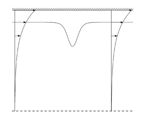
  $z\rightarrow -\infty$, respectively. A sketch of this physical problem is shown in figure 1. There is no assumption of irrotationality of the flow in the present model.

Figure 1. Sketch of a two-layer fluid system for the deep configuration.
2.1. Basic equations
In two dimensions, the mass conservation equations can be written as
 \begin{equation} \frac{{\partial {u_i}}}{{\partial x}} + \frac{{\partial {w_i}}}{{\partial z}} = 0\quad (i = 1,2), \end{equation}
where  $u$ and $w$ are the horizontal and vertical velocity components, respectively, $i=1$ stands for the lower-fluid layer and $i=2$ stands for the upper-fluid layer.
The momentum conservation equations for the upper- and lower-fluid layers can be written as
 $$\begin{gather} \frac{{\partial {u_i}}}{{\partial t}} + {u_i}\,\frac{{\partial {u_i}}}{{\partial x}} + {w_i}\,\frac{{\partial {u_i}}}{{\partial z}} ={-} \frac{1}{{{\rho _i}}}\,\frac{{\partial {p_i}}}{{\partial x}}\quad (i = 1,2), \end{gather}$$
 $$\begin{gather}\frac{{\partial {w_i}}}{{\partial t}} + {u_i}\,\frac{{\partial {w_i}}}{{\partial x}} + {w_i}\,\frac{{\partial {w_i}}}{{\partial z}} ={-} \frac{1}{{{\rho _i}}}\,{\frac{{\partial {p_i}}}{{\partial z}}} -g\quad (i = 1,2), \end{gather}$$
where  $t$ stands for time, $\rho _i$ is the mass density, $p_i$ is the pressure, and $g$ is the gravitational acceleration.
The kinematic boundary condition at the upper surface of the upper-fluid layer (rigid lid) can be written as
 \begin{equation} {w_2} = 0\quad \text{at}\ z=h. \end{equation}
The kinematic boundary conditions at the interface between the two fluid layers can be written as
 \begin{equation} {w_i} = \frac{{\partial \eta }}{{\partial t}} + {u_i}\,\frac{{\partial \eta }}{{\partial x}}\quad (i = 1,2)\quad \text{at}\ z=\eta(x,t). \end{equation}
The kinematic boundary condition at the bottom of the lower-fluid layer can be written as
 \begin{equation} {u_1}=0,\quad {w_1} = 0,\quad \text{when}\ z\rightarrow-\infty. \end{equation}
The dynamic boundary condition at the interface between the two fluid layers can be written as
 \begin{equation} {\bar p_2} = {\hat p_1}\quad \text{at}\ z=\eta(x,t), \end{equation}
where  $\bar p_2$ is the pressure at the lower surface of the upper-fluid layer, and $\hat p_1$ is the pressure at the upper surface of the lower-fluid layer.
Equations (2.1)–(2.6) are the basic equations for the two-layer fluid system in the deep configuration.
2.2. Equations for the deep-water two-layer HLGN model
In the traditional two-layer HLGN model (Zhao et al. Reference Zhao, Ertekin, Duan and Webster2016, Reference Zhao, Wang, Duan, Ertekin, Hayatdavoodi and Zhang2020), the undisturbed depths of the two fluid layers are both assumed to be finite. The velocity fields are expressed approximately by
 \begin{equation} {u_i}(x,z,t) = \sum_{n = 0}^{{K_i}} {{u_{n,i}}(x,t)\,z^n},\quad {w_i}(x,z,t) = \sum_{n = 0}^{{K_i}} {{w_{n,i}}(x,t)\,z^n}\quad (i = 1,2), \end{equation}
where  $u_{n,i}$ and $w_{n,i}$ are the unknown horizontal and vertical velocity coefficients, and $K_i$ is a positive integer that represents the level used for each layer.
In the present HLGN model, the undisturbed depth of the upper-fluid layer is still assumed to be finite. Hence a polynomial function is still utilized as the shape function to approximate the velocity field for the upper-fluid layer.
Since the undisturbed depth of the lower-fluid layer is assumed to be infinite, the product of the exponentials and polynomials is utilized as the shape function to approximate the velocity field for the lower-fluid layer. This shape function has been utilized to study one-layer deep-water problems efficiently (Webster & Kim Reference Webster and Kim1991; Zheng et al. Reference Zheng, Zhao, Duan, Ertekin and Chen2016).
The velocity fields are therefore expressed by
 $$\begin{gather} {u_{2}}(x,z,t) = \sum_{n = 0}^{{K_2}} {{u_{n,2}}(x,t)}\,{z^n},\quad {w_{2}}(x,z,t) = \sum_{n = 0}^{{K_2}} {{w_{n,2}}(x,t)}\,{z^n}, \end{gather}$$
 $$\begin{gather}{u_1}(x,z,t) = \sum_{n = 0}^{{K_1}} {{u_{n,1}}(x,t)}\,{{\rm e}^{{k}z}}\,{z^n},\quad {w_1}(x,z,t) = \sum_{n = 0}^{{K_1}} {{w_{n,1}}(x,t)}\,{{\rm e}^{{k}z}}\,{z^n}, \end{gather}$$
where  $k$ is the representative wavenumber that should be predetermined for a given case. We will discuss the selection of $k$ for calculating internal solitary waves later, in § 4.
We first consider the upper-fluid layer. Substituting (2.8a) into (2.1) with  $i=2$, we obtain
 $$\begin{gather} {u_{{K_2},2}} = 0, \end{gather}$$
 $$\begin{gather}{w_{n,2}} ={-} \frac{1}{n}\,\frac{{\partial {u_{n - 1,2}}}}{{\partial x}}\quad (n = 1,2,\ldots,K_2). \end{gather}$$
 Substituting (2.8a) into (2.2a) and (2.2b) with  $i=2$, multiplying each term by $z^n$ ( $n=0,1,\ldots, K_2$) and integrating from $h$ to $\eta$, will result in
 \begin{equation} {M_{n,2}} + \frac{{\left( {{\eta ^n} - {h^n}} \right)}}{{{\rho _2}}}\,\frac{{\partial {{\bar p}_2}}}{{\partial x}} = 0\quad (n = 1,2, \ldots ,{K_2}), \end{equation}
where
 $$\begin{gather} {M_{n,2}} = \frac{\partial }{{\partial x}}\left[ {{G_{n,2}} + g\left( {\int_h^\eta {{z^n}} \,{\rm{d}}z} \right)} \right] + n{E_{n - 1,2}} - {h^n}\left[ {{G_{0,2}} + g( {\eta - h} )} \right], \end{gather}$$
 $$\begin{gather}{E_{n,2}} = \sum_{m = 0}^{{K_2}} {\left\{ {\begin{array}{l} {\displaystyle\dfrac{{\partial {u_{m,2}}}}{{\partial t}}\left( {\int_h^\eta {{z^{m + n}}\,{\rm{d}}z} } \right) + \dfrac{{\partial {u_{m,2}}}}{{\partial x}}\left[ {\sum_{r = 0}^{{K_2}} {{u_{r,2}}\left( {\int_h^\eta {{z^{m + r + n}}\,{\rm{d}}z} } \right)} } \right]}\\ {\quad {}+ {u_{m,2}}\left[ {\displaystyle\sum_{r = 0}^{{K_2}} {{w_{r,2}}} \left( {m\int_h^\eta {{z^{m + r + n - 1}}\,{\rm{d}}z} } \right)} \right]} \end{array}} \right\}}, \end{gather}$$
 $$\begin{gather}{G_{n,2}} = \sum_{m = 0}^{{K_2}} {\left\{ {\begin{array}{l} {\displaystyle\dfrac{{\partial {w_{m,2}}}}{{\partial t}}\left( {\int_h^\eta {{z^{m + n}}\,{\rm{d}}z} } \right) + \dfrac{{\partial {w_{m,2}}}}{{\partial x}}\left[ {\sum_{r = 0}^{{K_2}} {{u_{r,2}}\left( {\int_h^\eta {{z^{m + r + n}}\,{\rm{d}}z} } \right)} } \right]}\\ {\quad {}+ {w_{m,2}}\left[ {\displaystyle\sum_{r = 0}^{{K_2}} {{w_{r,2}}} \left( {m\int_h^\eta {{z^{m + r + n - 1}}\,{\rm{d}}z} } \right)} \right]} \end{array}} \right\}} . \end{gather}$$
 We can eliminate  $\bar p_2$ by use of (2.10) with two different values of $n$, e.g. $n=1$ and $n=2$, $n=1$ and $n=3$, to obtain
 \begin{equation} ( {{\eta } - h} ){M_{n,2}} - ( {{\eta ^n} - h^n} ){M_{1,2}} = 0\quad (n = 2,3,\ldots,K_2). \end{equation}
Substituting (2.8a) into (2.3), we obtain
 \begin{equation} {w_{0,2}} ={-} \sum_{n = 1}^{{K_2}} h^n{{w_{n,2}}}. \end{equation}
 Substituting (2.8a) into (2.4) with  $i=2$, we obtain
 \begin{equation} \frac{{\partial \eta }}{{\partial t}} = \sum_{n = 0}^{{K_2}} {\eta}^{n}{\left( {{w_{n,2}} - \frac{{\partial \eta }}{{\partial x}}\,{u_{n,2}}} \right)}. \end{equation}
 Next, we consider the lower-fluid layer. Substituting (2.8b) into (2.1) with  $i=1$, we obtain
 $$\begin{gather} {u_{{{K_1},1}}} = {w_{{{K_1},1}}} = 0, \end{gather}$$
 $$\begin{gather}{w_{n,1}} ={-} \frac{1}{{{k}}}\left[ {\frac{{\partial {u_{n,1}}}}{{\partial x}} + ( {n + 1} ){w_{n + 1,1}}} \right]\quad (n={K_1}-1,{K_1}-2,\ldots,0). \end{gather}$$
 Substituting (2.8b) into (2.2a) and (2.2b) with  $i=1$, multiplying each term by ${\rm e}^{kz}\,z^n$ ( $n=0,1,\ldots, K_1-1$) and integrating from $-\infty$ to $\eta$, will result in
 \begin{equation} {M_{n,1}} + \frac{{{{\rm e}^{k\eta }}\,{\eta ^n}}}{{{\rho _1}}}\,\frac{{\partial {{\hat p}_1}}}{{\partial x}} = 0\quad (n = 0,1, \ldots ,{K_1} - 1), \end{equation}
where
 $$\begin{gather} {M_{n,1}} = \frac{\partial }{{\partial x}}\left[ {{G_{n,1}} + g\left( {\int_{ - \infty }^\eta {{{\rm e}^{kz}}\,{z^n}\,{\rm{d}}z} } \right)} \right] + k{E_{n,1}} + n{E_{n - 1,1}}, \end{gather}$$
 $$\begin{gather}{E_{n,1}} = \sum_{m = 0}^{{K_1} - 1} {\left\{\!{\begin{array}{@{}l@{}} {\displaystyle\dfrac{{\partial {u_{m,1}}}}{{\partial t}}\left( {\int_{ - \infty }^\eta {{{\rm e}^{2kz}}}\,{z^{m + n}}\,{\rm{d}}z} \right) + \dfrac{{\partial {u_{m,1}}}}{{\partial x}}\left[ {\displaystyle\sum_{r = 0}^{{K_1} - 1} {{u_{r,1}}\left( {\int_{ - \infty }^\eta {{{\rm e}^{3kz}}}\,{z^{m + r + n}}\,{\rm{d}}z} \right)} } \right]}\\ {\quad {}+ {u_{m,1}}\left[ {\displaystyle\sum_{r = 0}^{{K_1} - 1} {{w_{r,1}}\left( {\int_{ - \infty }^\eta {{{\rm e}^{3kz}}\left( {k{z^{m + r + n}} + m{z^{m + r + n - 1}}} \right)} \,{\rm{d}}z} \right)} } \right]}\end{array}} \right\}}, \end{gather}$$
 $$\begin{gather}{G_{n,1}} = \sum_{m = 0}^{{K_1} - 1} {\left\{\!{\begin{array}{@{}l@{}} {\displaystyle \dfrac{{\partial {w_{m,1}}}}{{\partial t}}\left( {\int_{ - \infty }^\eta {{{\rm e}^{2kz}}}\,{z^{m + n}}\,{\rm{d}}z} \right) + \dfrac{{\partial {w_{m,1}}}}{{\partial x}}\left[ {\displaystyle\sum_{r = 0}^{{K_1} - 1} {{u_{r,1}}\left( {\int_{ - \infty }^\eta {{{\rm e}^{3kz}}}\,{z^{m + r + n}}\,{\rm{d}}z} \right)} } \right]}\\ {\quad {}+ {w_{m,1}}\left[ {\displaystyle \sum_{r = 0}^{{K_1} - 1} {{w_{r,1}}\left( {\int_{ - \infty }^\eta {{{\rm e}^{3kz}}\left( {k{z^{m + r + n}} + m{z^{m + r + n - 1}}} \right)} \,{\rm{d}}z} \right)} } \right]}\end{array}} \right\}} . \end{gather}$$
 We can eliminate  $\hat p_1$ by use of (2.16) with two different values of $n$, e.g. $n=0$ and $n=1$, $n=0$ and $n=2$, to obtain
 \begin{equation} {M_{n,1}} - {\eta ^n}{M_{0,1}} = 0\quad (n=1,2,\ldots,{K_1}-1). \end{equation}
 Substituting (2.8b) into (2.4) with  $i=1$, we obtain
 \begin{equation} \frac{{\partial \eta }}{{\partial t}} = \sum_{n = 0}^{{K_1}} {{{\rm e}^{{k}\eta }}\,{\eta ^n}\left( {{w_{n,1}} - \frac{{\partial \eta }}{{\partial x}}\,{u_{n,1}}} \right)}. \end{equation}
We note that (2.5) always holds under the velocity field approximations in (2.8b).
Next, we couple the upper- and lower-fluid layers. Based on (2.6), we set  $n=1$ in (2.10) and set $n=0$ in (2.16) to obtain
 \begin{equation} {\rho _2}\,{{\rm e}^{{k}\eta }}\,{M_{1,2}} - {\rho _1}( {\eta - {h}} ){M_{0,1}} = 0. \end{equation}
 Finally, (2.12), (2.14) and (2.18)–(2.20) are the equations of the HLGN model. We can use (2.9b) and (2.13) to eliminate  ${w_{n,2}}$ ( $n=0,1,\ldots,K_2$), and use (2.15b) to eliminate ${w_{n,1}}$ ( $n=0,1,\ldots,K_1-1$). As a result, the unknowns are ${u_{n,2}}$ ( $n=0,1,\ldots,K_2-1$), ${u_{n,1}}$ ( $n=0,1,\ldots,K_1-1$) and $\eta$. The numbers of the equations and the unknowns are both $K_2+K_1+1$. Therefore, this system of equations is closed.
It should be noted that different values of  $K_2$ and $K_1$ in (2.8a) and (2.8b) correspond to different levels of the present HLGN model. For example, if we select $K_2=3$ and $K_1=5$, then we will establish the HLGN-P3E5 model, where ‘P’ is short for ‘polynomial’, and ‘E’ is short for ‘exponential’. When $K_1$ or $K_2$ increases, the dispersion performance of the present HLGN model becomes better, and this will be presented in the next subsection.
In this paper, a polynomial is utilized as the shape function for the upper-fluid layer of finite depth, and the product of polynomial and exponential is utilized as the shape function for the lower-fluid layer of infinite depth. If we rewrite the velocity approximations for the upper- and lower-fluid layers in a general form as
 \begin{gather} \qquad {u_i}(x,z,t) = \sum_{n = 0}^{{K_i}} {{u_{n,i}}(x,t)\,{\sigma _{n,i}}(z)},\quad {w_i}(x,z,t) = \sum_{n = 0}^{{K_i}} {{w_{n,i}}(x,t)\,{\sigma _{n,i}}(z)}\quad (i = 1,2), \end{gather}
where  ${\sigma _{n,i}}(z)$ is the general shape function utilized for each fluid layer, then one can establish the corresponding HLGN model following the derivation process presented in this paper. For example, the orthogonal polynomials (e.g. the Legendre function used for the upper-fluid layer of finite depth, and the Laguerre function used for the lower-fluid layer of infinite depth) can be utilized to further simplify the formulation due to their orthogonality and recursive properties, i.e. the terms related to the integrals of two shape function multiplications, $\int {{\sigma _{m,i}}(z)\,{\sigma _{n,i}}(z)\,{\rm {d}}z}$, can be simplified, but the much larger number of terms related to the integrals of three shape function multiplications, $\int {{\sigma _{m,i}}(z)\,{\sigma _{r,i}}(z)\,{\sigma _{n,i}}(z)\,{\rm {d}}z}$, cannot be simplified significantly.
2.3. Linear dispersion relations of the deep-water HLGN models for different levels
To validate the application range, the linear dispersion relations of the present HLGN models for different levels are studied in this subsection. Substituting the linear solutions of the horizontal-velocity coefficients  $u_{n,i}$ ( $n=0,1,\ldots,K_i-1$, $i=1,2$) and internal-wave profile $\eta$ to (2.12), (2.14) and (2.18)–(2.20), we can obtain the linear dispersion relations of the present HLGN models for different levels. We refer the reader to Webster et al. (Reference Webster, Duan and Zhao2011) for the derivation of the linear dispersion relations of the one-layer HLGN model for different levels in detail. Here, we fix $K_2=3$ since we find that it is enough to accurately describe the velocity fields for the upper-fluid layer of the internal solitary waves in the absence of shear-current considered in this paper (i.e. $K_2=3$ is the converged level for the upper-fluid layer).
Expressions for the linear dispersion relations of the first five levels of the HLGN models are given below.
HLGN-P3E1 model:
 \begin{equation} {\bar c^2} = \frac{{\left( {1 - \bar \rho } \right)}}{{\dfrac{1}{{15}}\,\bar \rho \left( {\dfrac{{{{\bar{k'}}^6} + 135{{\bar{k'}}^4} + 2880{{\bar{k'}}^2} + 6300}}{{{{\bar{k'}}^4} + 52{{\bar{k'}}^2} + 420}}} \right) + \dfrac{1}{2}\left( {\dfrac{{{{\bar k}^2} + {{\bar{k'}}^2}}}{{\bar k}}} \right)}}. \end{equation}
HLGN-P3E2 model:
 \begin{equation} {\bar c^2} = \frac{{\left( {1 - \bar \rho } \right)}}{{\dfrac{1}{{15}}\,\bar \rho \left( {\dfrac{{{{\bar{k'}}^6} + 135{{\bar{k'}}^4} + 2880{{\bar{k'}}^2} + 6300}}{{{{\bar{k'}}^4} + 52{{\bar{k'}}^2} + 420}}} \right) + \dfrac{1}{4}\left[ {\dfrac{{{{\bar k}^4} + 6{{\bar k}^2}{{\bar{k'}}^2} + {{\bar{k'}}^4}}}{{\bar k\left( {{{\bar k}^2} + {{\bar{k'}}^2}} \right)}}} \right]}}. \end{equation}
HLGN-P3E3 model:
 \begin{align} {\bar c^2} = \frac{{\left( {1 - \bar \rho } \right)}}{{\dfrac{1}{{15}}\,\bar \rho \left( {\dfrac{{{{\bar{k'}}^6} + 135{{\bar{k'}}^4} + 2880{{\bar{k'}}^2} + 6300}}{{{{\bar{k'}}^4} + 52{{\bar{k'}}^2} + 420}}} \right) + \dfrac{1}{2}\left[ {\dfrac{{{{\bar k}^6} + 15{{\bar k}^4}{{\bar{k'}}^2} + 15{{\bar k}^2}{{\bar{k'}}^4} + {{\bar{k'}}^6}}}{{\bar k\left( {3{{\bar k}^2} + {{\bar{k'}}^2}} \right)\left( {{{\bar k}^2} + 3{{\bar{k'}}^2}} \right)}}} \right]}}. \end{align}
HLGN-P3E4 model:
 \begin{align} {\bar c^2} = \frac{{\left( {1 - \bar \rho } \right)}}{{\dfrac{1}{{15}}\,\bar \rho \left( {\dfrac{{{{\bar{k'}}^6} + 135{{\bar{k'}}^4} + 2880{{\bar{k'}}^2} + 6300}}{{{{\bar{k'}}^4} + 52{{\bar{k'}}^2} + 420}}} \right) + \dfrac{1}{8}\left[ {\dfrac{{{{\bar k}^8} + 28{{\bar k}^6}{{\bar{k'}}^2} + 70{{\bar k}^4}{{\bar{k'}}^4} + 28{{\bar k}^2}{{\bar{k'}}^6} + {{\bar{k'}}^8}}}{{\bar k\left( {{{\bar k}^2} + {{\bar{k'}}^2}} \right)\left( {{{\bar k}^4} + 6{{\bar k}^2}{{\bar{k'}}^2} + {{\bar{k'}}^4}} \right)}}} \right]}}. \end{align}
HLGN-P3E5 model:
 \begin{align} {\bar c^2} = \frac{{\left( {1 - \bar \rho } \right)}}{{\dfrac{1}{{15}}\,\bar \rho \left( {\dfrac{{{{\bar{k'}}^6} + 135{{\bar{k'}}^4} + 2880{{\bar{k'}}^2} + 6300}}{{{{\bar{k'}}^4} + 52{{\bar{k'}}^2} + 420}}} \right) + \dfrac{1}{2}\left[ {\dfrac{{\left( {{{\bar k}^2} + {{\bar{k'}}^2}} \right)\left( {{{\bar k}^8} + 44{{\bar k}^6}{{\bar{k'}}^2} + 166{{\bar k}^4}{{\bar{k'}}^4} + 44{{\bar k}^2}{{\bar{k'}}^6} + {{\bar{k'}}^8}} \right)}}{{\bar k\left( {5{{\bar k}^4} + 10{{\bar k}^2}{{\bar{k'}}^2}{\rm{ + }}{{\bar{k'}}^4}} \right)\left( {{{\bar k}^4} + 10{{\bar k}^2}{{\bar{k'}}^2}{{ + 5}}{{\bar{k'}}^4}} \right)}}} \right]},} \end{align}
where the dimensionless linear-wave speed  $\bar c$, wavenumber $\bar {k'}$, representative wavenumber ${\bar k}$ and mass density $\bar \rho$ are
 \begin{equation} \bar c = \frac{c}{{\sqrt {gh} }},\quad \bar{k'} = {k'}h,\quad {{\bar k}} = {k}h,\quad \bar \rho = \frac{{{\rho _2}}}{{{\rho _1}}}. \end{equation}
Similar principles apply in obtaining the linear dispersion relations of the present HLGN models for higher levels (not shown here due to the complexity of the final relations).
The exact linear dispersion relation for internal gravity waves in this two-layer deep configuration is (Lamb Reference Lamb1932)
 \begin{equation} \bar c_{exact}^2 = \frac{{1 - \bar \rho }}{{\bar{k'}\left( {1 + \bar \rho \coth \bar{k'}} \right)}}. \end{equation}
 Figure 2 shows the relationship between the normalized wave speed squared  ${{\bar c}^2}/{\bar c_{exact}^2}$ and the wavenumber $\bar{k'}$ for the linear dispersion relations of the present HLGN models for different levels for the case $\bar \rho =0.952$ (Debsarma et al. Reference Debsarma, Das and Kirby2010). We observe that when $\bar k$ is not as close to $\bar {k'}$, such as when it is small (e.g. $\bar k/\bar {k'}=0.25$ shown in figure 2a) or large (e.g. $\bar k/\bar {k'}=4$ shown in figure 2e), the present HLGN models for lower levels have quite small application ranges. Under this condition, the present HLGN models for higher levels are required. When $\bar k$ is closer to $\bar {k'}$ (e.g. $\bar k/\bar {k'}=0.5$ shown in figure 2(b) and $\bar k/\bar {k'}=2$ shown in figure 2d), the application ranges of the present HLGN models for lower levels become significantly wider. Meanwhile, we observe that the HLGN-P3E3 model almost has the same application range compared with those of the HLGN-P3E4 and HLGN-P3E5 models. In particular, when $\bar k = \bar {k'}$, shown in figure 2(c), the HLGN models for different levels have the same and optimal application range. Meanwhile, from (2.22)–(2.26), we see that ${\bar {c}}^2 > 0$ since ${\bar {\rho }} < 1$, and when $\bar {k'}\rightarrow +\infty$, ${\bar {c}}^2\rightarrow 0$.

Figure 2. Relationship between the normalized wave speed squared  ${{\bar c}^2}/{\bar c_{exact}^2}$ and the wavenumber $\bar{k'}$ for the linear dispersion relations of the present HLGN models for different levels, $\bar \rho =0.952$: (a) $k/ {k'}=0.25$, (b) $k/ {k'}=0.5$, (c) $k/ {k'}=1$, (d) $k/ {k'}=2$, (e) $k/ {k'}=4$.
Furthermore, we compare the relationship between the normalized wave speed squared  ${{\bar c}^2}/{\bar c_{exact}^2}$ and the wavenumber $\bar{k'}$ for the linear dispersion relations of the HLGN-P3E5 model and other strongly nonlinear models, including the CC model (Choi & Camassa Reference Choi and Camassa1996a) and the DDK model (Debsarma et al. Reference Debsarma, Das and Kirby2010), for the case ${\bar \rho }=0.952$. The linear dispersion relations of the two strongly nonlinear models are as follows (see e.g. Debsarma et al. Reference Debsarma, Das and Kirby2010).
CC model:
 \begin{equation} {{\bar c}^2} = \frac{{1 - \bar \rho }}{{\bar \rho + \bar{k'}}}. \end{equation}
DDK model:
 \begin{equation} {\bar c^2} = \frac{{1 - \bar \rho }}{{\bar \rho \left( {\dfrac{{6{{\bar{k'}}^2} + 15}}{{{{\bar{k'}}^2} + 15}}} \right) + \bar{k'}}}. \end{equation}
 The comparison is shown in figure 3, where we observe that the application range of the CC model is  $\bar {k'}<0.74$ if the tolerable absolute error is $1-|{{\bar c}^2}/{\bar c_{exact}^2}| \leq 10\,\%$. The DDK model expands the application range to $\bar {k'}<5.15$. The application range of the HLGN-P3E5 model with $\bar k=\bar {k'}$ reaches $\bar {k'}<12.58$, and it has the widest application range among these models.

Figure 3. Relationship between the normalized wave speed squared  ${{\bar c}^2}/{\bar c_{exact}^2}$ and the wavenumber $\bar{k'}$ for the linear dispersion relations of the HLGN-P3E5 model and other strongly nonlinear models, $\bar \rho =0.952$.
3. Travelling solitary-wave solutions
We consider an internal solitary wave propagating from left to right with constant speed  $c$ and permanent wave profile in the presence of background shear-current shown in figure 4. We use the wave coordinates $XOZ$ located on the undisturbed interface between the two fluid layers and moving with the same speed $c$, where $X = x-ct$ and $Z=z$. Thus, we have the following relations:
 $$\begin{gather} \eta (x,t) = \eta (X),\quad {u_{n,i}}(x,t) = {u_{n,i}}(X)\quad (n = 0,1, \ldots ,{K_i} - 1, i=1,2), \end{gather}$$
 $$\begin{gather}\frac{\partial }{{\partial x}} = \frac{\rm{d} }{{{\rm d} {X}}},\quad \frac{\partial }{{\partial t}} ={-} c\,\frac{{\rm d} }{{{\rm d} {X}}}. \end{gather}$$
Substituting (3.1a) and (3.1b) into (2.12), (2.14) and (2.18)–(2.20) derived in the last section, the present two-layer HLGN equations for the travelling-wave solutions can be obtained.

Figure 4. Sketch of an internal solitary wave propagating in a two-layer fluid system in the deep configuration.
The focus of this paper is on internal solitary waves, requiring consideration of some geometric boundary conditions. Due to the symmetry, we need to consider only the front half of an internal solitary wave.
At the maximum displacement  $X=0$ (see figure 4), we have
 \begin{equation} \frac{{{\rm{d}}\eta }}{{{\rm{d}}X}} = 0,\quad \frac{{{\rm{d}}{u_{n,i}}}}{{{\rm{d}}X}} = 0\quad (n = 0,1, \ldots ,{K_i} - 1,\ i=1,2). \end{equation}
 At the far field  $X\rightarrow +\infty$ for the no-current cases, we have
 \begin{equation} \eta = 0,\quad {u_{n,i}} = 0\quad (n = 0,1, \ldots ,{K_i} - 1,\ i=1,2). \end{equation}
In the presence of the background shear-current, the current velocity profile  $u_c(Z)$ can be fitted by a polynomial function for the upper-fluid layer, and fitted by a product of polynomial and exponential functions for the lower-fluid layer, both using the least squares method, expressed as
 \begin{equation} {u_c}(Z) \approx \left\{ \begin{array}{@{}ll@{}} \displaystyle\sum_{n = 0}^{{{\tilde K}_2} - 1} {{{\tilde u}_{n,2}}} {Z^n}, & {\rm{for}}\ 0 \le Z \le h,\\ \displaystyle\sum_{n = 0}^{{{\tilde K}_1} - 1} {{{\tilde u}_{n,1}}}\,{{\rm e}^{kZ}}\,{Z^n}, & {\rm{for}}\ {- \infty} < Z \le 0, \end{array} \right. \end{equation}
where  ${\tilde u_{n,2}}$ ( $n = 0,1, \ldots,{\tilde K_2} - 1$) and ${\tilde u_{n,1}}$ ( $n = 0,1, \ldots,{\tilde K_1} - 1$) are the known fitted coefficients for the upper-fluid layer and lower-fluid layer, respectively. It should be noted that ${\tilde K_2} \leq K_2$ and ${\tilde K_1} \leq K_1$. Hence at the far field $X\rightarrow +\infty$ for the shear-current cases, we have
 \begin{equation} \eta = 0,\quad {u_{n,i}} = \left\{ \begin{array}{@{}ll@{}} {{\tilde u}_{n,i}} & (n = 0,1, \ldots ,{{\tilde K}_i} - 1,\ i = 1,2),\\[2pt] 0 & (n = {{\tilde K}_i},{{\tilde K}_i} + 1, \ldots ,{K_i} - 1,\ i = 1,2). \end{array} \right. \end{equation}
 The central finite-difference method is used to obtain the first, second and third spatial derivatives. The Newton–Raphson method is used to obtain the travelling-wave solutions. The initial values are obtained from the MCC model (Miyata Reference Miyata1985; Choi & Camassa Reference Choi and Camassa1999) for a very deep configuration where the depth ratio of the upper-fluid layer to the lower-fluid layer is  $1/99$. For the shear-current cases, we first obtain the solutions of internal solitary waves without any background shear-current. We then gradually increase the current strength to the desired value. Calculations are performed using Mathematica.
In order to assess whether the internal solitary wave obtained by the steady-solution algorithm can propagate over a flat bottom steadily, we have also established a time-domain algorithm for the present HLGN model. A five-point central-difference method of a uniform mesh is used to calculate the spatial derivations, and a fourth-order predictor–corrector Adams–Bashforth–Moulton scheme is used for time marching. A five-point smoothing filter is applied to effectively reduce the influence of the short waves and ensure stable propagation of large-amplitude internal waves over a long time. A similar but detailed numerical algorithm can be found in Zhao et al. (Reference Zhao, Wang, Duan, Ertekin, Hayatdavoodi and Zhang2020, Reference Zhao, Zhang, Duan, Wang, Guo, Hayatdavoodi and Ertekin2023).
The case parameters are  $\rho _2 / \rho _1 = 0.78$ and $a/h = 0.2$, $1.7955$ and $5$, where a is the amplitude of the internal solitary wave. The no-current cases are considered only. Initially, the maximum interface displacement of the internal solitary wave is located at $x/h = 0$. Snapshots of the internal solitary waves propagating at different moments obtained by the HLGN-P3E5 model are shown in figure 5. Meanwhile, we translate the internal-wave profiles at different moments to the place where the maximum displacement is at $x/h = 0$ in figure 6. From $t(g/h)^{0.5} = 0$ to $1000$, we observe that the internal-wave profiles show very good agreement, which indicates that the internal solitary waves can propagate steadily.

Figure 5. Snapshots of the internal solitary waves propagating at different moments (the maximum moment is  $t(g/h)^{0.5} = 1000$), with $\rho _2 / \rho _1 = 0.78$: (a) $a/h=0.2$, (b) $a/h=1.7955$, (c) $a/h=5$.

Figure 6. Translated internal solitary wave profiles at different moments, with  $\rho _2 / \rho _1 = 0.78$: (a) $a/h=0.2$, (b) $a/h=1.7955$, (c) $a/h=5$.
4. Numerical test cases
In this section, we will conduct some numerical tests to assess the accuracy of the HLGN model for deep configurations. First, we study the selection of the representative wavenumber  $k$ introduced in the present model, aiming to find a suitable value under which even the HLGN model for the lower level can obtain the converged results for a given case. Next, comparison is made between the HLGN model, the CC model, the DDK model and Euler's solution for internal solitary waves in the absence of background shear-current. Finally, comparison is made between the HLGN model and the DJL equation for internal solitary waves in the presence of background shear-current.
4.1. The effect of the representative wavenumber  $k$
$k$

In this subsection, we focus on the selection of the representative wavenumber  $k$ of the present HLGN model for calculating internal solitary waves. Here, we define the representative wavelength $\lambda = 2{\rm \pi} / k$. Koop & Butler (Reference Koop and Butler1981) introduced an integral measure of the effective wavelength, $\lambda _e$, which was defined as
 \begin{equation} {\lambda _e} = \left| {\frac{1}{a}\int_0^\infty {\eta (X)\,{\rm{d}}X} } \right|. \end{equation}
Many studies utilized (4.1) to obtain the relationship between the wave amplitude and effective wavelength (see e.g. Choi & Camassa Reference Choi and Camassa1999; Camassa et al. Reference Camassa, Choi, Michallet, Rusas and Sveen2006; Choi, Zhi & Barros Reference Choi, Zhi and Barros2020; Choi Reference Choi2022). Since, for a given case, the internal solitary wave profile  $\eta _{MCC}$ obtained by the MCC model can be calculated by solving (3.51) in Choi & Camassa (Reference Choi and Camassa1999), we can instantly obtain the effective wavelength $\lambda _{e\text {-}MCC}$ by use of (4.1), and set it as a reference value. According to this reference value, we can choose $\lambda$ of the present HLGN model.
Here, we consider some numerical cases whose parameters are given by Choi & Camassa (Reference Choi and Camassa1999) and Debsarma et al. (Reference Debsarma, Das and Kirby2010) as follows: the density ratio between the two fluid layers is  $\rho _2/\rho _1=0.78$, and the internal solitary-wave amplitude is $a/h=1.7955$. We note that only no-current cases are considered in this subsection. Under these parameters, we obtain $\lambda _{e\text {-}MCC}/h\approx 24$ for a very deep configuration where the depth ratio of the upper-fluid layer to the lower-fluid layer is $1/99$.
We first select  $\lambda /\lambda _{e\text {-}MCC}= 2$. Figure 7 shows the wave profile and velocity profile at the maximum interface displacement for different levels of the present HLGN model. In figure 7(b), $c_0$ is the linear long-wave speed in a two-layer fluid system ( $\rho _2<\rho _1$) for the deep configuration under the rigid-lid approximation, which is defined as
 \begin{equation} {c_0} = \sqrt {gh\left( {\frac{{{\rho _1}}}{{{\rho _2}}} - 1} \right)}. \end{equation}
It is noted that through our calculations, we find that  $K_2=3$ (given in (2.8a)) can provide sufficiently accurate velocity fields for the upper-fluid layer of finite depth in the absence of background shear-current. As a result, we change the value of $K_1$ (given in (2.8b)) only to perform the convergence test for the no-current cases.

Figure 7. Convergence test of the present HLGN models for different levels,  $\lambda = 2\lambda _{e\text {-}MCC}$, $\rho _2/{\rho _1}=0.78$ and $a/h=1.7955$: (a) wave profile; (b) velocity profile at the maximum interface displacement.
As shown in figure 7, we observe that the results of the wave profile and velocity profile at the maximum interface displacement obtained by the HLGN-P3E3 and HLGN-P3E1 models show some differences with those obtained by the HLGN-P3E5 and HLGN-P3E7 models, while the results obtained by the HLGN-P3E5 model and the results of the HLGN-P3E7 model show very good agreement. Thus it is concluded that when we select  $\lambda /\lambda _{e\text {-}MCC}= 2$, the HLGN-P3E5 model can provide the converged results for this case.
We also select  $\lambda /\lambda _{e\text {-}MCC}= 1$ and $4$ to perform the convergence tests of the present HLGN models for different levels. It is demonstrated that the HLGN-P3E9 model can provide converged results under the two different values of $\lambda$ for this case. Comparisons between the converged results of the present HLGN models for different $\lambda$ on wave profile and velocity profile at the maximum interface displacement are shown in figures 8(a) and 8(b), respectively.

Figure 8. Comparisons between the converged results of the present HLGN models with different representative wavelength  $\lambda$, $\rho _2/{\rho _1}=0.78$ and $a/h=1.7955$: (a) wave profile; (b) velocity profile at the maximum interface displacement.
From figure 8, we observe that the converged results of present HLGN model show very good agreement for different values of  $\lambda$. On the other hand, if we select the suitable one, $\lambda /\lambda _{e\text {-}MCC}= 2$, then we can obtain the converged results of the present HLGN model for the lower level (i.e. the HLGN-P3E5 model).
To further verify the suitable selection of  $\lambda /\lambda _{e\text {-}MCC}= 2$, we calculate an internal solitary wave with a larger amplitude $a/h=5$ (maximum amplitude considered in the present study) when the density ratio is still $\rho _2 / \rho _1 =0.78$. Under these parameters, we obtain $\lambda _{e\text {-}MCC}/h\approx 30$ for the deep configuration where the depth ratio of the upper-fluid layer to the lower-fluid layer is $1/99$. The convergence test of the present HLGN models for different levels on wave profile and velocity profile at the maximum interface displacement when $\lambda /\lambda _{e\text {-}MCC}= 2$ is shown in figure 9, where we again observe that the HLGN-P3E5 model can provide the convergence results.

Figure 9. Convergence test of the present HLGN models for different levels,  $\lambda = 2\lambda _{e\text {-}MCC}$, $\rho _2/{\rho _1}=0.78$ and $a/h=5$: (a) wave profile; (b) velocity profile at the maximum interface displacement.
In general, we find that the HLGN-P3E5 model with  $\lambda /\lambda _{e\text {-}MCC}= 2$ (i.e. $kh={\rm \pi} h/\lambda _{e\text {-}MCC}$) can provide the converged results for the no-current cases considered in this paper. In the next subsection, we will use the present HLGN-P3E5 model for the calculations.
4.2. Comparison between the present HLGN model and other models for internal solitary waves in the absence of background shear-current
In this subsection, we apply the present HLGN model to large-amplitude internal solitary waves in the absence of background shear-current in the deep configuration with two density ratios. The first case is  $\rho _2 / \rho _1 = 0.952$, which is used by Debsarma et al. (Reference Debsarma, Das and Kirby2010), and the other case is $\rho _2 / \rho _1 = 0.78$, which is used by Choi & Camassa (Reference Choi and Camassa1999) and Debsarma et al. (Reference Debsarma, Das and Kirby2010). The wave profile, velocity profile at the maximum interface displacement and wave speed are studied. For comparison purposes, results of the HLGN model are compared with those obtained by the DDK model and the CC model. We also use the numerical code developed by Rusas (Reference Rusas2000) to obtain Euler's solution. The algorithm of this numerical code is given in Grue et al. (Reference Grue, Jensen, Rusas and Sveen1999). The ratio of the upper-fluid layer depth to the lower-fluid layer depth is $1/99$ in all Euler's solutions shown in the following cases.
4.2.1. Case I: $\rho _2 / \rho _1 = 0.952$

We first consider the case  $\rho _2 / \rho _1 = 0.952$. The relationships between the wave speed and wave amplitude obtained by the HLGN model, the DDK model, the CC model and Euler's solution are shown in figure 10.

Figure 10. Relationship between the wave speed and wave amplitude,  $\rho _2/{\rho _1}=0.952$.
From figure 10, we observe that the CC model underestimates the wave speed for a given amplitude compared with Euler's solution. When the amplitude increases, the calculation error of the CC model becomes larger. The DDK model can describe the wave speed accurately when the wave amplitude is small. When the wave amplitude becomes larger, the DDK model overestimates the wave speed. In general, the wave speed calculated by the present HLGN model match Euler's solution very well even when the wave amplitude is large.
Next, we focus on the wave profile. Following Debsarma et al. (Reference Debsarma, Das and Kirby2010), we consider the internal solitary waves with amplitudes  $a/h= 0.875$ and $1.884$. Results of the present HLGN model, the DDK model, the CC model and Euler's solution on wave profile are shown in figure 11.

Figure 11. Wave profile,  $\rho _2/{\rho _1}=0.952$: (a) $a/h=0.875$, (b) $a/h=1.884$.
From figure 11, we observe that the wave profile obtained by the present HLGN model show very good agreement with Euler's solution. On the other hand, the CC model obtains the narrower wave profile, and the DDK model obtains the wider profile compared with Euler's solution.
The velocity profiles at the maximum interface displacement obtained by the HLGN model and Euler's solution are shown in figure 12. From figure 12, we observe that the HLGN results match Euler's solution very well, for both the upper-fluid layer and the lower-fluid layer.

Figure 12. Velocity profile at the maximum interface displacement,  $\rho _2/{\rho _1}=0.952$: (a) $a/h=0.875$, (b) $a/h=1.884$.
4.2.2. Case II: $\rho _2 / \rho _1 = 0.78$

Now we consider the case  $\rho _2 / \rho _1 = 0.78$. The relationships between the wave speed and wave amplitude obtained by different models are shown in figure 13.

Figure 13. Relationship between the wave speed and wave amplitude,  $\rho _2/{\rho _1}=0.78$.
From figure 13, we observe again that the DDK model overestimates the wave speed and the CC model underestimates the wave speed when the amplitude is relatively large. The wave speed obtained by the HLGN model matches Euler's solution well even when the wave amplitude reaches  $a/h=4.5$.
Then we consider the profiles of internal solitary waves with amplitudes  $a/h= 1.7955$ and $5$. Due to the absence of the CC and DDK results in the existing literature for amplitude $a/h = 5$, to be used for comparisons, we have written the code to obtain the numerical results of the CC and DDK models. We first validate the accuracy of the code that we developed for this purpose for the CC and DDK models. Figure 14 shows the comparison between the present numerical results of the CC and DDK models, and the results that we capture from Debsarma et al. (Reference Debsarma, Das and Kirby2010) for the case $a/h = 1.7955$ and $\rho _2/{\rho _1}=0.78$, where perfect agreement is observed. This is an indication that our code for the CC and DDK models is accurate.

Figure 14. Comparison between the present numerical results of the CC model and the DDK model and the results given by Debsarma et al. (Reference Debsarma, Das and Kirby2010),  $a/h = 1.7955$ and $\rho _2/{\rho _1}=0.78$.
Results of the HLGN model, the DDK model, the CC model and Euler's solution on wave profile are shown in figure 15, where we observe that the present HLGN model shows better agreement with Euler's solution compared with the results of the DDK and CC models.

Figure 15. Wave profile,  $\rho _2/{\rho _1}=0.78$: (a) $a/h=1.7955$, (b) $a/h=5$.
Figure 16 shows the relationship between the effective wavelength and the wave amplitude, which can be obtained by using (4.1). The results of the HLGN model again match Euler's solution very well even when the amplitude reaches  $a/h=5$. For further discussion on the relationship between the effective wavelength and the amplitude when the amplitude approaches the maximum value, we refer the reader to Camassa et al. (Reference Camassa, Choi, Michallet, Rusas and Sveen2006).

Figure 16. Relationship between the effective wavelength and wave amplitude,  $\rho _2/{\rho _1}=0.78$.
Comparisons between the results of the HLGN model and Euler's solution for the velocity profile at the maximum interface displacement of two amplitudes of internal solitary waves are shown in figures 17(a) and 17(b), respectively. We again observe that the HLGN results match Euler's solution remarkably well.

Figure 17. Velocity profile at the maximum interface displacement,  $\rho _2/{\rho _1}=0.78$: (a) $a/h=1.7955$, (b) $a/h=5$.
To demonstrate the cost of running different models, we apply the HLGN-P3E5 model, the CC model, the DDK model and the numerical method for solving Euler's equations to calculate the internal solitary wave with  $a/h = 1.7955$ when $\rho _2/{\rho _1}=0.78$. All calculations are performed on a computer equipped with a Xeon(R) W-11855M CPU @ 3.20 GHz and 32 GB of memory. The Newton–Raphson method, as mentioned in § 3, is applied to solve the nonlinear equations. The number of discrete nodes for describing the half-profile of the internal solitary wave is $300$. The HLGN-P3E5 model, the CC model and the DDK model are implemented by Mathematica using our own code, while Euler's solution is obtained by Matlab in Rusas (Reference Rusas2000). It should be noted that the results provided by the CC model should be obtained in advance for the DDK model (Debsarma et al. Reference Debsarma, Das and Kirby2010). Table 1 shows the CPU times for these models.
Table 1. CPU times for the different models for calculating internal solitary waves,  $a/h=1.7955$ and $\rho _2/{\rho _1}=0.78$.

From table 1, it is demonstrated that the CPU time of the CC model and the DDK model is relatively short, while the HLGN model requires longer computational time. The HLGN model, however, can be used to study the wave–current interaction, wave–wave interaction and wave–topography interaction, which go beyond the capabilities of Euler's solution (Rusas Reference Rusas2000) used in this comparison.
4.3. Comparison between the present HLGN model and the DJL equation for internal solitary waves in the presence of background shear-current
In this subsection, we will conduct some numerical tests to assess the accuracy of the HLGN model for the internal solitary waves in the presence of background shear-current for the deep configuration. The density ratio between the two fluid layers is selected as  $\rho _2/\rho _1=0.952$. The amplitude of the internal solitary wave is fixed at $a/h=0.5$. Under these parameters, we determine the representative wavenumber as $kh = {\rm \pi}h/{\lambda _{e\text {-}MCC}} \approx 0.133$. We select the velocity profile of the background shear-current as the exponential form
 \begin{equation} {u_c}(Z) = U\,{{\rm e}^{{k_c}Z}}, \end{equation}
where  $U$ is the current speed at the undisturbed interface between the two fluid layers, and $k_c$ is a real number.
We first consider the case where  $U/c_0=1$ and $k_c/k=1$ (i.e. $k_ch=0.133$). We apply (3.4) with $\tilde {K}_2=3$ and $\tilde {K}_1=1$ to fit this velocity profile of the current, which can be written as
 \begin{equation} {u_c}(Z)= {c_0}\,{{\rm e}^{0.133({Z}/{h})}} \approx \left\{ \begin{array}{@{}ll@{}} {c_0}\left( {1 + 0.133\,\dfrac{Z}{h}+0.00885\,\dfrac{Z^2}{h^2}} \right), & \text{for}\ 0\leq Z \leq h,\\ {c_0}\,{{\rm e}^{0.133({Z}/{h})}}, & \text{for} \ {-\infty} < Z \leq 0. \end{array} \right. \end{equation}
Comparisons of the velocity profile between the fitted background shear-current and the desired background shear-current for the upper- and lower-fluid layers are shown in figures 18(a) and 18(b), respectively, where good agreement is observed.

Figure 18. Comparisons of the velocity profile between the fitted background shear-current and the desired background shear-current in the two-layer fluid system,  $U/c_0=1$ and $k_ch=0.133$: (a) upper-fluid layer; (b) lower-fluid layer.
We apply the HLGN-P5E7 model to obtain the converged results of the HLGN model for all the cases in this section. For comparison purposes, we also obtain the results of the DJL equation by using the open-source solver given by Dunphy, Subich & Stastna (Reference Dunphy, Subich and Stastna2011). It should be noted that in the DJL open-source solver, the velocity profile of the background shear-current is not necessarily fitted. Meanwhile, since the DJL equation considers the continuous density-stratified condition, we set the depth of the pycnocline as very small (i.e. 0.1 % of the total depth), and the depth ratio between the upper-fluid layer and lower-fluid layer as approximately 1/99.
The wave profile and the velocity profile at the maximum interface displacement obtained by the HLGN model and the DJL equation are shown in figures 19(a) and 19(b), respectively. We observe that the results obtained by the HLGN model show good agreement with those obtained by the DJL equation.

Figure 19. Comparison between the results obtained by the HLGN model and the DJL equation,  $\rho _2/{\rho _1}=0.952$, $a/h=0.5$, $U/c_0=1$ and $k_ch=kh=0.133$: (a) wave profile; (b) velocity profile at the maximum interface displacement.
Figures 20(a) and 20(b) show the wave profile and the velocity profile at the maximum interface displacement obtained by the HLGN model and the DJL equation for the case  $U/c_0=-1$, where good agreement is also found. It is also shown that the wave profile is much narrower for the case $U/c_0=-1$ than that for the case $U/c_0=1$.

Figure 20. Comparison between the results obtained by the HLGN model and the DJL equation,  $\rho _2/{\rho _1}=0.952$, $a/h=0.5$, $U/c_0=-1$ and $k_ch=kh=0.133$: (a) wave profile; (b) velocity profile at the maximum interface displacement.
Then we apply the same approach to study the case  $k_c=2k$ (i.e. $k_ch=0.266$). Taking the case $U/c_0=1$ as an example, we use (3.4) with $\tilde {K}_2=3$ and $\tilde {K}_1=3$ to fit this velocity profile of the current, which can be written as
 \begin{align} {u_c}(Z)={c_0}\,{{\rm e}^{0.266({Z}/{h})}} \approx \left\{ \begin{array}{@{}ll@{}} {c_0}\left( {1 + 0.266\,\dfrac{Z}{h}+0.03538\,\dfrac{Z^2}{h^2}} \right), & \text{for}\ 0\leq Z \leq h,\\ {c_0}\,{{\rm e}^{0.133({Z}/{h})}}\left( {0.96442{{ + }}0.09891\,\dfrac{{Z}}{h} + 0.00264\,\dfrac{{{Z^2}}}{{{h^2}}}} \right), & \text{for} \ {-\infty} < Z \leq 0. \end{array} \right. \end{align}
Comparisons of the velocity profile between the fitted background shear-current and the desired background shear-current for the upper- and lower-fluid layers are shown in figures 21(a) and 21(b), respectively, where we observe that the fitted results still match the desired results well.

Figure 21. Comparisons of the velocity profile between the fitted background shear-current and the desired background shear-current in the two-layer fluid system,  $U/c_0=1$ and $k_ch=0.266$: (a) upper-fluid layer; (b) lower-fluid layer.
Figures 22 and 23 show the results obtained by the HLGN model and the DJL equation for the cases  $U/c_0=1$ and $U/c_0=-1$, respectively. Good agreement is found between the HLGN results and the DJL results in general.

Figure 22. Comparison between the results obtained by the HLGN model and the DJL equation,  $\rho _2/{\rho _1}=0.952$, $a/h=0.5$, $U/c_0=1$ and $k_ch=2kh=0.266$: (a) wave profile; (b) velocity profile at the maximum interface displacement.

Figure 23. Comparison between the results obtained by the HLGN model and the DJL equation,  $\rho _2/{\rho _1}=0.952$, $a/h=0.5$, $U/c_0=-1$ and $k_ch=2kh=0.266$: (a) wave profile; (b) velocity profile at the maximum interface displacement.
5. Conclusions
To improve the efficiency of the traditional two-layer HLGN model for describing large-amplitude internal waves in deep water, a new two-layer HLGN model is established for a two-layer fluid system where the depth of the upper-fluid layer is finite while the depth of lower-fluid layer is infinite. In the present HLGN model, polynomials are utilized to approximate the velocity distribution in the vertical direction of the upper-fluid layer, while products of the exponentials and polynomials are utilized to approximate the velocity distribution in the vertical direction of the lower-fluid layer. Large-amplitude internal solitary waves in the absence and presence of background shear-current in the deep configuration are studied numerically. Comparison of the results between the HLGN model and other strongly nonlinear models is carried out to validate the accuracy of the present HLGN model. The conclusions are outlined below.
(i) By analysing the linear dispersion relations of the present HLGN models for different levels, we find that the selection of the representative wavenumber
$k$ leads to different application ranges of the HLGN model. If one selects a suitable $k$, then the HLGN model with the lower level can also offer an acceptable application range. Compared with the CC model derived by Choi & Camassa (Reference Choi and Camassa1996a) and the DDK model derived by Debsarma et al. (Reference Debsarma, Das and Kirby2010), it is shown that the application range of the HLGN-P3E5 model with $k={k'}$ (where ${k'}$ is the wavenumber) can reach ${k'}h<12.58$, which is wider than ${k'}h<5.15$ of the DDK model and ${k'}h<0.74$ of the CC model.(ii) For calculating internal waves in the absence of background shear-current, we have studied the selection of the representative wavenumber
$k$. Through the calculations, we find that $kh={\rm \pi} h/ \lambda _{e\text {-}MCC}$, where $\lambda _{e\text {-}MCC}$ is the effective wavelength obtained by the MCC model for the depth ratio of the upper-fluid layer to the lower-fluid layer as $1/99$ for a given case, may be a good choice. Under this parameter, the HLGN-P3E5 model can provide the converged results of the present HLGN model for the no-current cases considered in this paper.(iii) We utilize the present HLGN model to obtain the wave profile, velocity profile at the maximum interface displacement and wave speed for large-amplitude internal solitary waves in the absence of background shear-current in the deep configuration. By comparing with the results provided by the CC model and the DDK model, the results obtained by the HLGN model show better agreement with Euler's solution.
(iv) We also utilize the present HLGN model to obtain the wave profile and velocity profile at the maximum interface displacement for internal solitary waves in the presence of background shear-current in the deep configuration. The results obtained by the HLGN model show good agreement with those obtained by solving the DJL equation.


We note that due to the assumption of inviscid fluid and immiscibility between the upper and lower fluids and the velocity field approximations, the present HLGN model is unable to account for some phenomena such as the breaking of internal waves; see e.g. Carr et al. (Reference Carr, Franklin, King, Davies, Grue and Dritschel2017) for capturing the viscous effects and boundary layer mechanics. The development of the present HLGN model for dealing with these problems is left for future work.
Acknowledgements
The authors are grateful to Professor J. Grue and Dr T.J. Ellevold of the Department of Mathematics, University of Oslo, Norway, for providing the numerical code ‘IW2 (Two-layer Internal Waves)’ to help us to obtain Euler's solution. The corresponding author thanks Dr R.P. Li of the School of Engineering, Westlake University for fruitful discussions. The authors are also grateful to the anonymous referees for their comments that improved the quality of the paper.
Funding
The work of the first, second, third and seventh authors (B.Z, T.Z, Z.W. and W.D.) is supported by the National Natural Science Foundation of China (nos 12202114, 52261135547), the China Postdoctoral Science Foundation (no. 2022M710932), the State Key Laboratory of Coastal and Offshore Engineering, Dalian University of Technology (no. LP2202), the Fundamental Research Funds for the Central Universities (no. 3072022FSC0101), the Qingdao Postdoctoral Application Project, the Heilongjiang Touyan Innovation Team Program, and the PhD Student Research and Innovation Fund (no. BCJJ2023103).
Declaration of interests
The authors report no conflict of interest.


