


1. Introduction
In the United States, Social Security Old-Age Insurance, often referred to as simply ‘Social Security’, offers workers a choice: they can start receiving reduced benefits as early as age 62 or delay claiming up until age 70, resulting in higher monthly benefits for the rest of their life. Claiming early means a worker receives benefits for more years since he or she starts receiving them sooner, but their monthly benefit is actuarially adjusted downward. Therefore, what's best for an individual or a couple? It depends on: how long a worker and their spouse expect to live; how long he or she is able to work; what other resources the household can one draw on; and their plans and goals for the remaining years of life. Advocates for delaying claiming, including academics and financial planners, argue that low interest rates and improved longevity make delaying actuarially advantageous (Shoven and Slavov, Reference Shoven and Slavov2014) or that delaying insures against outliving one's resources (Williams, Reference Williams2020). Others highlight claiming early can facilitate enjoying financial resources while still healthy (Lambert, Reference Lambert2020). Largely absent from this discussion is evidence of the long-term outcomes of early claimants (i.e., those claiming at age 62), including how they fare financially as they age. We provide evidence by tracking early claimants through their late 70s; data are not yet available for tracking at later ages.
A simple comparison of early claimants with later claimants using data from the Health and Retirement Study (HRS) – a nationally representative panel survey of households with one member aged 50 and older – shows that early claimants have substantially less liquid wealth and lower household income in their 70s.Footnote 1 However, many differences pre-date the claiming decision: for example, those who claim early have lower income, on average, than later claimants when both were age 60, and later financial differences may reflect these pre-existing differences. We match married early claimants with married later claimants who were otherwise similar at age 60, and compare the decisions and financial well-being of both groups as they both age. Although this matching process does not replicate an experimental setting to establish the causal effect of claiming early, it allows us to estimate how financial circumstances in retirement among early claimants differ from otherwise similar individuals who postponed claiming. Our main findings comparing matched early claimants to later claimants with similar characteristics in their early 60s are:
(1) early claimants stop working earlier and cash out defined contribution (DC) pension plans sooner,
(2) early claimants have lower household income from 62 through their 70s (on average, $14,000 less in annual household income),
(3) early claimants in their 70s have less liquid wealth than later claimants at similar ages (on average, 27% lower), but these differences are only marginally statistically significant, and
(4) measures of financial hardship and mortality rates are not statistically or substantively different into their 70s.
There are two main limitations to our analysis. First, our data do not allow us to track households into their 80s. The relative advantage of claiming later grows substantially in claimants' 80s, and we must wait for additional years of follow-up data to determine whether differences in financial well-being widen. Second, individuals we observe in their late 70s claimed in the 1990s or early 2000s, and thus faced a lower penalty for early claiming than for more recent cohorts, and more recent cohorts are living longer. Therefore, someone turning 62 today has a stronger incentive to delay claiming than the cohorts under study in this analysis, all else equal.
Our findings suggest that the difference between early and later claimants in financial well-being at later ages can largely be attributed to differences in these groups that preceded the claiming decision itself. These two groups differ substantially, demographically, and financially, as well as in their health status, at age 60. We account for these differences through a matching process, and we further exclude Social Security Disability Insurance applicants, in order to focus on the tradeoffs in the retirement claiming decision among otherwise similar households. We find that claiming early is associated, albeit not strongly statistically significantly, with a number of other financially impactful decisions: for many households, income drops and remains lower, and liquid wealth lags behind that of similar households that claimed later. However, early claiming is not associated with a number of clearly negative outcomes, including mortality and financial hardship, suggesting that personal preference for leisure plays a role in claiming and retirement choices. Future research, following these households into their 80s, may uncover additional consequences of early claiming for financial wealth, responses to adverse health shocks, and well-being at advanced ages.
2. Why claim early? The tradeoffs in choosing when to claim
Social Security-covered workers can receive their full monthly benefit – their primary insurance amount (PIA) – when they reach their full retirement age (FRA), which is currently 66 and is slated to rise to 67 over the next few years. However, workers have the option to claim as early as age 62, the earliest eligibility age). But, claiming early carries penalties: monthly benefits are permanently reduced. Workers claiming at 62 with an FRA of 66 receive only 75% of their PIA per month for the rest of their lives. Furthermore, beneficiaries younger than their FRA are subject to the retirement earnings test, temporarily withholding a portion of their benefits if they continue to work and have earnings above a given threshold while receiving benefits.
However, claiming early means more years of receiving benefits, and the shorter one expects to live, the more advantageous it is to claim early. As extreme examples, if one expects to die at age 63, then there is no personal advantage in delaying claiming until age 66.Footnote 2 On the contrary, if one expects to live until 106, the 25% lower benefits over 40 years is a greater loss than the gain of receiving reduced benefits four years earlier.Footnote 3
Prior to 2008, Social Security Administration claims representatives used a ‘break-even age’ calculator, which allowed an individual to calculate the age at which living longer meant claiming at the FRA was more financially advantageous than claiming at age 62. Research shows that break-even framing influences individuals to claim Social Security benefits earlier compared to alternative framings such as framing delayed claiming as a gain, loss (Dominitz et al., Reference Dominitz, Hung and van Soest2007, Liebman and Luttmer, Reference Liebman and Luttmer2012), or even a more neutral framing (Brown et al., Reference Brown, Kapteyn and Mitchell2016). However, even if one had an accurate prediction of one's own mortality, calculating a break-even age is even more complicated: for a variety of reasons, some individuals may value money much less in the future than today, which makes claiming later less attractive. Figure 1 illustrates this point by comparing the break-even age for someone who values future benefits the same as today (i.e., no discount) and someone who values the real value of future benefits at a 5% discount per year relative to benefits received today (i.e., 5% discount). By discounting future benefits by 5%, the break-even age is pushed back from age 77 to 87.

Figure 1. Comparison of lifetime benefits by age of death at age 62 for alternative claiming ages and rates of discounting future values.
Notes: Figure assumes PIA of $1,000, leading to monthly benefits of $1,000 if benefits are claimed at age 66 and $750 if benefits are claimed at age 62. Social Security benefits are indexed for inflation and so benefits remain constant in real terms.
A few other factors may also influence a person's decision to delay claiming benefits. If he or she has other assets that could be used to finance claiming later, the decision of when to claim benefits should compare the guaranteed rate of return from delaying Social Security benefits relative to the expected rate of return on these assets. If the expected and potentially risky return from those assets is lower than the lifetime gains from delayed claiming, then the person should delay claiming and begin drawing down these lower-return assets instead. Conversely, if an individual turning 62 is in debt, especially high-interest debt, or if they would have to take on debt if they were not receiving Social Security benefits, then claiming early may result in an improved financial situation. Finally, if an individual is married, then his or her claiming choices can impact the benefit their spouse receives before and after their death.
But, perhaps the most important factor in deciding when to claim surrounds retirement, by which we mean when one stops working, which can be a different age than when one claims Social Security benefits. Claiming at age 62 can be a vital source of support for individuals seeking to retire as early as possible but who lack the resources to do so, those who are already out of the labor force with limited income, or those who recently lost a job, had to take on caregiving responsibilities, or have an overly demanding job. However, if one can continue to work and delay claiming, then monthly benefits rise not just because of a later claiming age but also because of additional earnings.Footnote 4 PIAs are based on earnings histories, and if workers are earning at a relatively high level in their 60s, then continuing to work will raise their Social Security benefits even faster than delaying claiming alone. If pension entitlements or contributions continue to grow with later retirement ages, then the payoffs to retirement wealth from retiring and claiming later can grow substantially. Indeed, proponents of delayed claiming, be they academic researchers or financial advisors, point toward the pairing of delayed claiming and delayed retirement as the driver of increased monthly Social Security benefits (Shoven and Slavov, Reference Shoven and Slavov2014; Goda et al., Reference Goda, Ramnath, Shoven and Slavov2018; Backman, Reference Backman2020).Footnote 5
Ultimately, the choice of when and how to start drawing on retirement wealth, including Social Security wealth, is personal, depending, in large part, on a person's (and potentially their spouse's) plans for retirement. For example, individuals in declining health may prioritize retirement and spending in their early 60s over higher monthly payments in their 70s. However, Social Security Old-Age Insurance is exactly that: a form of insurance against a worker and his or her spouse outliving their other resources. Retirees rely more on these benefits as they age. For example, Dushi et al. (Reference Dushi, Iams and Trenkamp2017) estimate that in 2014, 42% of 65- to 69-year-olds rely on Social Security for at least half of their income, but 61% of those over the age of 80 rely on Social Security for at least half of their income. Furthermore, there is increasing evidence that individuals are too ‘pessimistic’ about their personal life expectancy; they live longer than they expect to live (Bissonnette et al., Reference Bissonnette, Hurd and Michaud2017; d'Uva et al., Reference d'Uva, O'Donnell and van Doorslaer2017). We may, thus, be concerned that even if individuals fully understand the tradeoffs in claiming Social Security early, they may nevertheless underweight the insurance value of these benefits if they live longer than they expect. The implication is that individuals who claim early are forced to draw down other forms of wealth sooner than they would otherwise, risking poverty in older age.
Despite the wide range of studies documenting the characteristics of early claimants and trends in early claiming (Burkhauser et al., Reference Burkhauser, Couch and Phillips1996; Li et al., Reference Li, Hurd and Loughran2008; Shoven and Slavov, Reference Shoven and Slavov2012; Munnell and Chen, Reference Munnell and Chen2015; Hou et al. Reference Hou, Munnell, Sanzenbacher and Li2017; Purcell, Reference Purcell2020), there has been remarkably little evidence on how early claimants fare after claiming. That is, as the years of permanently lower benefits go by, how are they doing financially relative to if they had delayed claiming?
3. Approach
Although evaluating the consequences of claiming at age 62 has important implications for the financial security of older Americans and how their federal government should present information about the claiming decision, it has not been evaluated primarily because a randomized controlled trial, the gold standard for evaluation, is impractical. The evaluation period would need more than a decade of follow-up, detailed surveys would need to be conducted to assign appropriate treatment (i.e., age-62 claimants) and control groups (post-age-62 claimants), and participants would have to agree to abide by random selection into treatment and control groups understanding selection may lead to long-term financial differences and may constrain future choices (e.g., ability to afford future vacations and leave bequests). Randomization is required because we expect, and as discussed below researchers have consistently found, that individuals claiming at age-62 differ in systematic ways from those who delay claiming. For situations where randomized controlled trials are infeasible, the statistical, economic, and health literatures have developed a variety of quasi-experimental approaches aimed at approximating randomization into treatment and control groups (see Imbens and Wooldridge, Reference Imbens and Wooldridge2009, for a review). Matching is one such approach and the one we pursue here.
Matching uses data-capturing pre-treatment characteristics to connect observationally similar treated individuals to control individuals. Underlying our matching approach is the assumption that, after controlling for observable factors, if individuals who claimed at age 62 had opted to delay claiming, then their outcomes are unbiasedly estimated by the outcomes of their matched control delayed claimants. That is, there is no selection into early claiming that is not accounted for by pre-claiming observed characteristics. Randomization is one method of achieving this lack of selection, but is not a necessary condition for achieving what, in the literature, is known as unconfoundedness. The ‘random’ decision-making may reflect factors we cannot observe (e.g., use of rules-of-thumb and influence of friends and family). If the decision to claim at 62 is unconfounded after controlling for these factors, then the observable differences in outcomes, be they financial, health, or other well-being measures, represent the consequences of claiming early. As described above, there is a mechanical consequence of claiming early – one's Social Security benefit will be permanently lower. After the decision to claim at 62, individuals will likely make innumerable more decisions that may compensate or exacerbate the permanently lower lifetime benefit. For example, after claiming early an individual might choose less expensive leisure activities, thereby lowering their routine costs. Our interest, and we believe the interest of policymakers and Americans who will be making this choice in the future, is whether financial, health, or other well-being outcomes are persistently, statistically, and meaningfully different for age-62 claimants. We expect some persistent differences to arise, for example, in the Social Security benefit. This is neither concerning nor surprising. Of concern would be persistent differences indicating the decision to claim at 62 was a ‘bad’ choice, in that it made the average age-62 claimant worse off – for example, running out of savings or having insufficient resources to support care in old age. If evidence of ‘bad’ choices arises, then it would suggest a potential role for policymakers, the Social Security Administration or other stakeholders in developing interventions that might address the long-term negative outcomes.
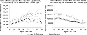
Key to our analytic approach is matching individuals who claim Social Security at different ages, but who are otherwise similar directly before claiming. Early claimants differ not just in terms of prior income, as shown in Figure 2, but along a number of health, employment, and sociodemographic dimensions. Armour and Knapp (Reference Armour and Knapp2021) document how age-62 claimants systematically differ from those who delay claiming.

Figure 2. Average levels of household liquid wealth or household income, married couples, by claimant type, ages 52–80.
Source: Authors' calculations from Health and Retirement Study interviews. No adjustments are made for observable differences between the two groups. Limited to households married in interview wherein husband was aged 60 or 61. Households with wives older than husbands excluded from sample. The 95% confidence intervals are shown in dotted lines. Sample size is 2,524 including 864 age-62 claimants. See Appendix A for additional details on sample selection.
Consistent with prior research on early claiming (Burkhauser et al., Reference Burkhauser, Couch and Phillips1996; Li et al., Reference Li, Hurd and Loughran2008), we found that the early claimant population is a diverse one. Some predictive factors of early claiming are related to those who otherwise do not have many resources to draw on: lower-paid workers, the non-employed, individuals living in rural areas, those with less education, and those in jobs that require physical effort. However, a substantial fraction of early claimants appears to be financially secure and are already retired: those already receiving other pension income and those covered by employer-provided retiree health insurance are also more likely to claim earlier.
4. Data
Given the impracticality of conducting a randomized experiment, the finding that age-62 claimants differ in substantive ways from post-age-62 claimants supports a matching approach. In order to implement matching, we require substantial panel data that tracks individuals over time including their Social Security claiming decisions as well as other financial, employment, household, demographic, and health characteristics.
We use the Health and Retirement Study (HRS), which provides more than two decades of data on individuals and their households (for this study, 1992–2016, although it continues to today). The HRS is a nationally representative survey of the US population over the age of 50 and their partners or spouses. It is also a panel survey that follows the same individuals over time and re-interviews them every 2 years, allowing researchers to track respondents as they leave the labor force and enter retirement and it captures financial, employment, household, demographic, and health characteristics.
5. Methodology
We use nearest-neighbor matching, whereby we match every age-62 claimant to a post-age-62 claimant (with replacement)Footnote 6 with values of the key characteristics that are as close as possible, otherwise known as that age-62 claimant's ‘nearest neighbor’. The advantage of this approach is that otherwise disparate early claimants are matched to a later claimant most similar to them, not just to a claimant with a similar likelihood to claim earlyFootnote 7; although an unemployed, rural resident with a work-limiting health condition and a city-dweller with retiree health insurance and current pension income may have similar likelihoods of claiming early, and hence be likely to be matched under a propensity score approach, they differ dramatically and make for a ‘noisy’ match. Such individuals are highly unlikely to be considered nearest neighbors, leading to an estimation process with less variance through comparing more similar individuals.
Drawing on Imbens (Reference Imbens2014), we formalize our matching approach – let E i = 1 if individual i is an age-62 claimant and E i = 0 otherwise. The observed outcome (e.g., liquid wealth and household income) for individual i at time t is

where $Y_{i, t}^{obs}$ is used to denote what is observed (e.g., we do not observe Y i,t(1) if E i = 0). For each individual there are X i possible explanatory factors. Therefore, we observe $( {Y_{i, t}^{obs} , \;\;E_i, \;X_i} )$
 . The average treatment effect on the treated (ATET) is then defined as:

There are two key assumptions: overlap and unconfoundedness. Overlap requires that for a given set of explanatory factors, that there exists a non-zero and non-one probability of being in the treatment group:

Unconfoundedness requires that, conditional on the explanatory factors, the treatment is independent:

Rubin (Reference Rubin2005) and Imbens (Reference Imbens2014) highlight a three-stage process for flexibly and robustly estimating the average effects of a treatment. First, the design stage assesses the overlap between the treated and control groups – in our case, age-62 claimants and post-age-62 claimants. Overlap ensures that matched individuals actually have similar characteristics. The design stage determines the final sample. Second, an assessment of the unconfoundedness assumption. Finally, the differences in outcomes can be assessed for the trimmed sample and interpreted based on the limitations determined in the first two stages.
5.1. Design and sample selection
In the design stage, the focus is to ensure that age-62 claimants look like post-age-62 claimants. Armour and Knapp (Reference Armour and Knapp2021) highlight key dimensions along which age-62 claimants differ from later claimants – these include marital and disability status, employment, and the receipt of pension income immediately prior to age-62. A typical lifecycle model of a forward-looking individual based on initial conditions such as these would yield different claiming decisions (Hurd et al., Reference Hurd, Smith and Zissimopoulous2004; Knapp, Reference Knapp2014). In order to focus on how households' finances and decisions change over time across early claimants and those who claim later, we focus on HRS respondents who will rely on Social Security retirement benefits and thus face the choice of whether to claim at age 62 or postpone claiming. We accomplish this by restricting the HRS sample in the following ways:
(1) Restrict to respondents observed before and after they reach age 62 in order to observe their characteristics prior to age 62 and whether they claimed at age 62.
(2) Exclude respondents who received Social Security benefits before the age of 62 (typically, recipients of non-retirement benefits, such as survivor or disability benefits), as well as those who have applied for Social Security Disability Insurance (DI) benefits at ages 60–62 and thus may still be in the initial determination or appeals process.Footnote 8
(3) Exclude respondents where eligibility for Social Security retirement or spousal benefits at age 62 could not be determined.
Appendix A provides a detailed accounting of our sample selection.
For this sample, the relevant Social Security choice is what age to claim Social Security retirement benefits, and we observe the characteristics of both early and later claimants before and after age 62. These characteristics include a rich array of sociodemographic, financial, employment, family structure, and health measures that can be used for matching. We specifically draw on these variables in the interview before a potential claimant turns 62, which, given the biennial nature of the HRS, means these measures are recorded at either age 60 or 61, but to which we will refer to as age 60 measures from here onward.
From this sample, we create subsamples for analysis based on marital status, spousal age, and employment immediately prior to age 62, which are key remaining characteristics for ensuring accurate matches. Since resources are typically shared within a household and Social Security provides benefits to spouses of beneficiaries, the structure of a household (i.e., married couple, divorced, widowed, or never married individual) will play a critical role in the respondent's claiming decision. For our main analytical sample, we focus on the largest subsample: married men who are the same age or older than their wives and who are working at age 60. The focus on married individuals reflects that 79% of our sample are married at age 60.Footnote 9 The focus on married men reflects that marriage for the purposes of Social Security is restricted to opposite sex couples and within these couples Social Security benefits are generally based on the husband's work history. The focus on married men that are the same age or older than their wives ensure their claiming decision is not influenced by prior claiming decisions of the wife – 88% of married men are the same age or older than their wife in our final sample. Finally, the focus on married men that are working at age 60 is because they represent a larger and distinct group from those that are not working. As noted in other places (Hurd et al., 2004; Armour and Knapp, Reference Armour and Knapp2021), individuals not working prior to age 62 are more likely to be receiving pension income or have a working limiting condition.Footnote 10 Our final analytic subsample consists of 2,524 age-60 individuals before matching.
Although our main analysis will focus on the subsample of married men that are the same age or older than their wives and are working at age 60, we extend our analysis to alternative groups in online Appendix B. These alternative groups have smaller sample sizes and hence poorer match quality, so our ability to make inferences is limited. Nevertheless, it provides interesting context on the potential generalizability of our findings based on our main analytical subsample that could be addressed with larger samples in the future.
Before describing our nearest-neighbor matching design, we first examine gross differences in trajectories of major financial security measures. We focus on our main analytic subsample and two financial measures in particular: liquid household wealthFootnote 11 and total household income.Footnote 12 One concern among proponents of claiming later is that the option to claim early also incentivizes earlier retirement which can lead to drawing down other forms of wealth sooner. As a result, early claimants would have both lower monthly Social Security payments and lower wealth in terms of other retirement resources in old age. We expect these drawdowns to be most apparent in more liquid forms of wealth. Figure 2 provides mean values of these financial measures as well as 95% confidence intervals for married couples in which the husband claimed at age 62 versus couples where the husband postponed claiming.
As the first panel of Figure 2 shows, age-62 claimants have persistently lower liquid wealth but it grows at roughly similar rates as later claimants between ages 52 and 60. Starting at age 62, growth in mean wealth diverges, with later claimants continuing to grow their wealth while early claimant's liquid wealth plateaus. By age 70, later claimants have significantly and substantially more liquid wealth. Although this pattern is consistent with earlier claimants needing to draw down their resources faster to make ends meet, it may also reflect underlying preferences: perhaps those who claim early also planned to settle into a lower-cost lifestyle.
The second panel of Figure 2 shows that age-62 claimants also have persistently lower income. Both early and late claimants exhibit relatively stable household income through age 60, and then incomes decline throughout the 60s, with age-62 claimants exhibiting an earlier decline in income, likely associated with earlier retirement.
Figure 2 highlights the motivation for matching. The long-run income and wealth patterns that we see may reflect pre-existing differences. The question then arises as to the extent to which pre-existing differences between early claimants and later claimants account for long-run differences in their wealth or income. The goal of designing a successful match is identifying key characteristics, such as liquid wealth and household income, that can capture original differences between age-62 claimants and post-age-62 claimants.
We use sociodemographic characteristics and measures of financial resources and health as explanatory factors for our matching estimator. All income and wealth variables are in 2016 dollars, adjusted with the CPI-U-RS.Footnote 13 In total, we match individuals on the characteristics at age 60 (the last interview before turning 62 and being eligible for Social Security Old-Age Insurance) included in Table 1. Specific definitions are discussed in Appendix A. Table 1 presents a restrictive match, which are the explanatory factors using in the matching estimator for our main analysis, and a less restrictive match that we use in online Appendix B when examining alternative subsamples (e.g., divorced women and married men not working at age 60) where an increase in sample size is necessary. Using a more restrictive matching reduces the sample size by requiring more exact matches. The tradeoff for the smaller sample size is that the remaining matches tend to be more balanced.
Table 1. Age 60 characteristics used for matching early claimants to later claimants, married households with older, employed husbands

a Annual earnings, liquid wealth (less restrictive match only), and net housing wealth were matched not on value, but on which quintile of said real value the individual was in among all age 60/61-year-olds. Distance was calculated with inverse diagonal sample covariance matrices.
As noted above, we use a nearest-neighbor matching approach. For some discrete characteristics, as noted in Table 1, we use exact matching. Exact matching requires that a potential post-age-62 claimant have the exact same characteristics as an age-62 claimant. After exact matching is applied, the nearest neighbor within each set of exact matches is determined by the match that has the smallest distance.Footnote 14 Our matching estimator includes a bias adjustment (Abadie and Imbens, Reference Abadie and Imbens2006) that uses linear regression to remove biases associated with differences between age-62 claimants and post-age-62 claimants that persist after the initial match. Factors included in the regression adjustment are separately noted in Table 1.
Choice of which characteristics to exactly match are based on factors that appear to differentially effect claiming choice, including race, location, household income, pension income, and liquid wealth. Since it is impossible to exactly match on continuous measures, such as income and wealth, we first categorize these measures, then proceed to exact match on those categories and include the continuous measure when finding the smallest distance.Footnote 15 Implementing this approach reduces our sample size from 2,524 individuals to 1,524 individuals of which 572 claim at age-62. Subsequent analyses will be based on this subsample.
The main goal of the matching process is to ensure similar distributions of measured baseline characteristics between the treated and untreated groups (Austin, Reference Austin2009). Balance can be measured by differences in the explanatory factors after matching, but as balance is meant to reflect the entire distribution of the covariates, matching on higher order moments is preferred (Austin, Reference Austin2009; Linden and Samuels, Reference Linden and Samuels2013). Comparison of post-match differences in age-60 characteristics, as presented in Table 2, can be statistically different but substantively small. Prior research has deemphasized t-statistic testing, like that in Table 2, in favor of comparing standardized differences in the explanatory factors (Imbens, Reference Imbens2014) as well as variance ratios (VRs) between treatment and control groups (Austin, Reference Austin2009; Linden and Samuels, Reference Linden and Samuels2013). These are unitless approaches that are not influenced by sample size. Next, we use two statistics to assess balance at the design stage: standardized differences and VRs of the explanatory factors at age 60. Later, in the analysis stage, we can also assess intertemporal balance by examining pre-trends in the outcomes of interest.
Table 2. Age 60/61 household characteristics and differences with matched later claimants
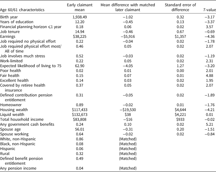
Notes: Sample size = 1,524; number claiming at 62 = 572.
Source: Author's calculations.
Table 3 contains information on the quality of the matching process by comparing pre-match and post-match standard differences and VRs. Ideally, standardized differences would be zero, and VRs equal to 1. No formal tests exist, although researchers have proposed a number of ad hoc diagnostics (Austin, Reference Austin2009). Linden and Samuels (Reference Linden and Samuels2013) note standardized differences in excess of 0.1–0.25 have been potentially indicative of imbalance. Imbens (Reference Imbens2014) used a benchmark of 0.3. Using an absolute difference of 0.25 as a benchmark, Table 3 indicates significant pre-match imbalances in birth year, years of education, individual earnings, DC entitlement, and total household income. After the match, these imbalances fall below our benchmark, except now any government cash benefits is imbalanced. Later, we will investigate if any government cash benefits at age 60 is indicative of claiming at 62 after conditioning for other observable factors (it is not). If we were to use a tighter benchmark of 0.1, some additional differences would remain, including birth year, years of education, financial planning horizon, earnings, expected likelihood of living to 75, and the probability of being in fair health, and housing wealth. It is important to identify whether these differences are substantively important. Returning to Table 2, we see that the most concerning of these, individual earnings, corresponds to a $5,900 annual difference, which is a substantively small difference. The differences in Table 2 of the other measures appear to be substantively small as well, with the exception of the probability of fair health, with individuals claiming at 62 to be twice as likely to report being in fair health (15% versus 7%). Next, we assess the VRs, an indicator of whether or not variance of age-62 claimants is similar to later claimants for each of the explanatory factors. Here again, prescribed benchmarks vary. Rubin (Reference Rubin2001) describes VRs outside 0.5 and 2 as extreme, and aims to have most VRs fall within 0.8 and 1.25. Using this benchmark, the sample is initially imbalanced on birth year, earnings, job requiring physical effort, the probability of having fair or excellent health, liquid wealth, household income, the probability of receiving any government cash benefits, and pension income. After the match, most of these are within our benchmarks, with imbalance on fair health and any government cash benefits remaining, and poor health, financial planning horizon and expected likelihood of living to 75 arising. From these diagnostics, we conclude that our sample is well balanced except on the following characteristics at age 60: probability of poor or fair health, receipt of any government cash benefits, financial planning horizon, and expected likelihood of living to 75. In the next subsection, we assess whether any of these factors are indicative of claiming at 62 after conditioning for other observable factors.
Table 3. Standardized differences and VRs between raw and matched age 60/61 households

Notes: Sample size = 1,524; number claiming at 62 = 572.
Source: Author's calculations.
5.2. Assessment of unconfoundedness assumption
Although the unconfoundedness assumption is not testable, Imbens (Reference Imbens2014) suggests calculations for assessing its plausibility. Recall the unconfoundedness assumption requires that, conditional on the explanatory factors, the treatment is independent:

where E i represents the claiming decision at age-62 and X i represent observable characteristics at age-60 (as noted in Table 1). We partition X i into two parts: pseudo-outcomes $( {X_i^p } )$ and the remaining explanatory factors $( {X_i^r } )$
 . To assess the plausibility of the unconfoundedness assumption, we test if the pseudo-treatment after conditioning on our remaining explanatory factors is zero: ${\rm {\opf E}}[ {X_i^p ( 1 ) -X_i^P ( 0 ) \vert E_i = 1, \;X_i^r } ] = \hat{\tau }_{ATET}^p = 0$
 . Intuitively, we are estimating the causal effect of age-62 claiming behavior on prior choices after conditioning on other explanatory factors. Since current behavior cannot cause past outcomes, we expect this to be zero. Imbens (Reference Imbens2014) suggests that if true, statistically and substantively, then this can be interpreted as supportive of the unconfoundedness assumption. This stage offers an assessment of the credibility of the next stage's analyses without using the outcomes of interest.
When thinking about confoundedness, we are particularly concerned with latent factors that could affect the claiming decision and the outcome of interest. If an individual's claiming decision is representative of a latent factor (e.g., preference for leisure), then we would expect pseudo-treatment test to be violated. Although many of the explanatory factors in Table 1 could be used as pseudo-outcomes, we focus on a limited number that have particularly conceptual interest in that we would expect them to correspond with latent factors: preference for leisure, forward-looking behavior, survival duration, and resource constrained.
Table 4 compares possible latent factors to their pseudo-outcomes and reports our estimates of the effect of claiming at age 62 on the pseudo-outcomes. This is done for the pseudo-outcomes and control factors at age 60. If our explanatory factors were insufficient to explain unobserved differences in preference for leisure, then a typical lifecycle model would lead us to expect that they would accumulate differential wealth (liquid or otherwise) by claiming status. If age-62 claimants had a higher preference for leisure, then we would expect greater wealth accumulation. As reported in Table 4, we find small and insignificant differences for liquid wealth and total net wealth (the sum of liquid wealth and illiquid wealth, including housing, business, and vehicles, less debt).
Table 4. Assessment of unconfoundedness assumption

If age-62 claimants were less likely to engage in forward-looking behavior, then we would expect lower savings rates and a greater likelihood of reporting a financial planning horizon of 1 year or less. As noted in Table 4, we find small and insignificant differences for liquid wealth and the probability of having a short financial planning horizon.
If age-62 claimants had differential longevity expectations, we would expect a lower self-reported probability of living to age 75. We do find that age-62 claimants have a self-reported probability of living to 75 that is 4 percentage points lower than later claimants. This casts doubt on the unconfoundedness assumption. In reviewing the distribution of subjective survival to age 75, we find that age-62 claimants with self-reported probabilities of living to 75 below 50% are particularly difficult to match on. In Appendix B, we restrict our main analysis sample to only those individuals with a 50% self-reported probability of living to age 75 (i.e., forcing an exact match on these characteristics) as a sensitivity analysis and find that our key findings hold. An alternative framing of survival expectations would be individuals who are in poor or fair health would be more likely to claim at age 62 because poorer health puts them at greater risk of having an unexpectedly short life. In Table 4, we find small and insignificant differences for poor and fair health.
Finally, we observed that age-62 claimants or their spouses were more likely to be receiving some government benefits at age 60 (e.g., receiving unemployment benefits), suggesting a possible need for resources. Here, again we find small and insignificant differences in Table 4 after accounting for other observable factors are age 60.
6. Analysis
Now that we have identified that our matching estimator has done a good job of ensuring overlap and the unconfoundedness assumption generally holds, we turn to using our matching model to assess the outcomes of interest. First, we consider expected outcomes – namely, differences in Social Security income and employment. These should largely reflect mechanical pathways: higher initial Social Security income/lower employment rates initially, and then, as later claimants retire and collect their benefits, lower Social Security income and similar employment rates. The expected outcomes reassure us that the matching is having the intended effect. Second, we consider key retirement outcomes, including sources of retirement income, wealth, and other indictors of potential long-run differences, including mortality and financial hardship. These are the outcomes of most interest, as these address how, as the years of permanently lower benefits go by, are age-62 claimants doing financially relative to if they had delayed claiming.
6.1. Social security income and employment among early claimants
Figure 3 presents differences between early claimants and later claimants by age for two outcome variables: Social Security income and employment. The first panel shows differences in annual Social Security income between early claimants and matched later claimants as a function of age, as well as 95% confidence intervals. This panel is both a validity of whether our analysis is successful – our early claimants should be receiving Social Security income earlier than our later claimants, after all – but it also presents an opportunity to describe how we present the results of our analysis in an intuitive context.

Figure 3. Average difference in husband's annual social security retirement income and employment between age-62 claimants and matched controls, 2016 dollars, married households, by age of husband.
Each panel shows estimates of the difference between matched early claimants and later claimants by husband's age, although given that HRS interviews are every other year, age 60 refers to ages 60 or 61, age 62 to ages 62 or 63, and so on. We can continue to follow individuals as they age, although the sample size falls the farther past age 62 we follow them: we observe all respondents at age 60 and 62 by construction, but as we follow people into their 70s, our sample is limited to those born earlier and earlier since we do not observe anyone past the 2016 HRS interview. As a result, our sample skews toward those born earlier the longer we follow individuals into older age.
The solid black line shows the estimated difference between early claimants and later claimants at that age, with 95% confidence intervals from our estimation shown as dashed lines. Across all of our analyses, we would like there to be no ‘pre-trends’ in these graphs: that is, our matching process is intended to match similar individuals. By construction they are similar at age 60, since we match with variables evaluated at that age, but the more similar the pre-age-60 characteristics, the more confident we are in the validity of our match. Individual may attrit from our sample due to three types of non-response: mortality, survey censoring (e.g., age occurring before first interview or after last interview), or survey attrition. Should either individual in a match be non-responsive at a given age, their outcomes are no longer included in the estimates. This means that for our ATET estimates if the later claimant becomes non-responsive, the age-62 claimant is matched to their next-best match. If an age-62 claimant becomes non-responsive, then their contribution to the ATET estimate is dropped.Footnote 16
The first panel of Figure 3 shows the most obvious distinction between age-62 claimants and matched individuals who claimed later: no difference in annual Social Security income before age 62, then, at age 62, substantially higher Social Security income for early claimants.Footnote 17
The spike begins to decline at the FRA, ranging from ages 65 to 66 for this cohort, where later Social Security claimants start claiming their benefits. Indeed, by age 68, when all respondents are older than their FRA, this difference has disappeared, and for these married men, self-reported annual Social Security income is statistically significantly lower for early claimants than for later claimants, consistent with higher monthly benefits from delayed claiming. We note that the analogous figures for all other household types also show the same pattern, although the statistical significance of lower Social Security income for early claimants at older ages varies across household type.
The first panel of Figure 3 is a mechanical result of a successful analytic construction: early Social Security claimants receive Social Security income earlier. The second panel of Figure 3 presents the average change in another outcome: whether the respondent is employed. By construction, we have limited the sample of earlier and later claimants to those working at age 60, but we do not observe any differences in employment before age 60 (which we did not explicitly match on; an ‘out-of-sample’ test), supporting the validity of our match.
Upon claiming benefits, there is a dramatic decline in employment for these early claimants relative to their matched counterparts who delayed claiming: relative to later claimants, age-62 claimants were 40 percentage points more likely to stop working. Since we condition only on age-60 characteristics, we cannot speak to whether individuals left their jobs because they claimed benefits and were discouraged from work through the earnings test or taxability of Social Security benefits, or claimed benefits because they left their jobs and needed other sources of income. However, in online Appendix B, we conduct parallel analyses on married households wherein the husband was neither in poor health nor had a work-limiting health condition at age 60 or at age 62. This limitation is intended to exclude individuals who suffered a health shock, and thus may have been induced to both leave employment and claim benefits. The difference in employment is nearly identical (40 percentage points in Figure 3; 39 percentage points for no-shock households, Appendix Figure B3). This finding is consistent with benefit receipt itself leading to less work (i.e., early claimants would work longer in the absence of age-62 benefits); however, although we match on the physical and psychological difficulty of jobs, earnings, job tenure, and pension entitlements, a portion of these early claimants may have lower unmeasured job satisfaction or a higher unmeasured preference for leisure (i.e., desire to not work) than later claimants who continue to work. This lower attachment to the labor force is underscored by the difference in employment remaining statistically significant for much of the claimants' 70s. That is, both early and later claimants are receiving Social Security benefits (and, as the first panel shows, later claimants are receiving more in Social Security benefits, on average), but later claimants are still statistically significantly more likely to be working.
6.2. Retirement outcomes
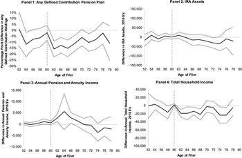
We now turn to differences in retirement outcomes. First, we consider four measures of retirement resources and income between these early claimants and matched control claimants, shown in the four panels of Figure 4: any DC plan assets (e.g., 401(k)) in the household, average household individual retirement account (IRA) assets, average household income from pensions and annuities, and total household income. These resources reflect decumulation or restructuring of retirement resources, and, ultimately, income at the household's disposal.

Figure 4. Average difference in income and retirement resources between age-62 claimants and matched controls, 2016 dollars, married households, by age of husband.
From prior analyses, we found that those who postpone claiming were more likely to have DC plan assets at age 60. Here, our matching process corrected for that difference at and before that age. But, another pattern arises: early claimants were substantially less likely (by 16 percentage points) to have a DC plan at age 62 after they have claimed. What explains this difference? One possibility is that employers can force workers leaving their employment to cash out their low-balance plans (i.e., plans with less than $5,000 in assets), and since we see substantial exits from employment for early claimants, perhaps these forced cash-outs or rollovers explain exit. However, additional analyses limited to plans worth at least $5,000, not shown here for the sake of brevity, show nearly identical drops – indicating that ‘forced cash outs’ do not explain the differences observed here.
Early claimants may be rolling over these DC balances into IRAs (thereby increasing IRA balances), cashing them out (thereby increasing pension or annuity income or increasing savings), or purchasing annuities. There is no evidence of rolling over DC balances into IRAs (panel 2) but the third panel is consistent with the cash-out explanations: income from pensions and annuities show statistically significant increases. That is, those claiming Social Security early have more pension/annuity income at ages 62 than those who claim Social Security later. These patterns are consistent with workers who tap into their Social Security wealth early also restructuring and drawing on their other retirement assets at the same time. Prior research has found a similar pattern for individuals who face later FRAs: they postpone not just Social Security claiming, but also retirement and pension decumulation (Armour and Hung, Reference Armour and Hung2017).Footnote 18 Although Social Security claiming, non-Social Security pension receipt, and retirement from work are all separate decisions, they are often interrelated through incentives or individuals' perceptions, and individuals claiming Social Security early also tend to start receiving other pensions and stop working early.
Since early claimants, relative to later claimants, have lower earnings from earlier retirement, but higher income from Social Security, pensions, and annuities, the question arises as to the overall difference in income as both groups age. As the IRA and pension and annuity income figures indicate, the higher values for early claimants do not persist much past 62 and by the 70s, they are lower on average, albeit insignificantly different from zero. We, thus, examine differences in total household income to determine the net effect of all of these differences over time.
From the fourth panel of Figure 4, we find that, starting at age 62, early claimant households have less household incomeFootnote 19 than those that postponed claiming. Since early claimants are substantially more likely to retire, it is not surprising that total income falls: a common rule of thumb is to aim for retirement income to be 80% of pre-retirement income (Marksjarvis, Reference Marksjarvis2016; Fedweek, 2017). Since average household income is approximately $83,800 in real terms at age 60 for early claimants (see Table 2), the magnitude of the age 62 decline is broadly consistent with this rule of thumb (78%). Indeed, cash expenditures (especially, non-health-related expenditures) decline upon retirement, even as other measures of consumption do not, since retired households can substitute purchases for home production (e.g., substituting eating lunch at home versus eating at a restaurant; see Hurd and Rohwedder, Reference Hurd and Rohwedder2008).
However, this difference in income persists; from ages 74 to 76, household income for age-62 claimants is $23,000 lower than for later claimants; this difference is substantial relative to early claimants' income, since, as shown in Figure 2, 76-year-old early claimants receive $54,000 in household income, on average. Since nearly all respondents are no longer working by this age, this difference represents lower retirement income itself, even though pre-claiming income was similar across groups. This difference could be intentional, if early claimants are electing to retire early and use their available resources earlier in retirement. But, the fact remains that compared to otherwise similar individuals who postponed claiming, age-62 claimants continue to have substantially less income at these older ages.
Figure 5 compares differences in mortality and liquid wealth between the two claiming groups. The central tradeoff of choosing when to claim Social Security is that claiming earlier results in lower monthly benefits, but one has access to them sooner. The older one expects to live, the less advantageous early claiming is. Although analyses with administrative data have long shown that those who claim at age 62 are more likely to die sooner than those who delay claiming (Rader et al., Reference Rader, Reno and Upp1982), such comparisons do not account for pre-existing differences in health or other characteristics. In this analysis, we are not only comparing those who claim at 62 with those who delay claiming, but also comparing individuals who match on a number of characteristics, including expected likelihood of living to at least age 75, in the year before reaching age 62.
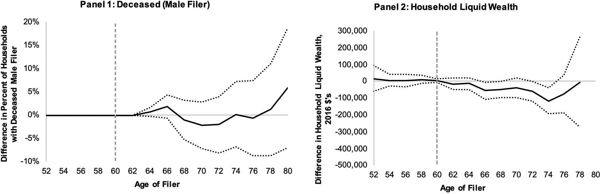
Figure 5. Difference in mortality and liquid wealth between age-62 claimants and matched controls, 2016 dollars, married households, by age of husband.
We find that there is not a significant difference in mortality, statistically or otherwise, between early claimants and matched later claimants. That is, the pre-62 characteristics used to match cases appear to account for any differences in mortality, at least through age 80. On the one hand, this result is encouraging: we know income is lower for these individuals from panel 4 of Figure 4, but this lower level of resources is not reflected in higher mortality, as it is in other Social Security contexts, such as Social Security Disability Insurance (Gelber et al., Reference Gelber, Moore and Strand2017). On the other hand, the advantages to claiming later increase with life expectancy, and these early claimants appear no more likely to die sooner than comparable later claimants. However, strong conclusions are difficult, since although the point estimate on differences in mortality is close to zero, the confidence interval is quite large, preventing the rejection of substantial differences in either direction.
Although a permanent income provides for routine needs, accumulated liquid wealthFootnote 20 is important for unexpected large expenses that permanent income flows may be insufficient to cover (e.g., large medical bills and major household repairs). To determine whether there is a resulting decline in broader financial resources besides income, we turn to our measure of liquid wealth to answer the question of whether early claiming is associated with having fewer resources in older age than similar individuals who claimed later have.
As the second panel shows, until claimants' mid-60s, liquid wealth is not any lower for age-62 claimants than later claimants. Starting at age 66, it is insignificantly lower for age-62 claimants. Only at age 74, do early claimants have statistically significantly less wealth than later claimants – approximately $115,000 less. From Figure 2, comparisons of liquid wealth between unmatched early claimants and later claimants demonstrated that differences arose not from a large decline in wealth for the age-62 claimants, but continued growth in later claimants' wealth. The majority of these later-in-life differences are explained by age 60 characteristics. The remaining differences could be the result of lower Social Security benefits themselves being only sufficient for routine expenses and thus preventing further accumulation of resources. Conversely, these differences could be indicative of over-savings or income in excess of need on the part of later claimants.
From their 60s onward, early claimants have less household income than otherwise similar later claimants, and lower liquid wealth that is declining relative to later claimants. These differences are substantial: mean liquid wealth among age-62 claimants ranges from $162,000 to $200,000 between ages 70 and 78 for our matched sample, which is an average 27% less in liquid wealth than their matched counterparts.Footnote 21 Those who claimed early are drawing down their wealth. They are, therefore, entering their 80s with lower liquid resources and permanently lower monthly Social Security benefits from early claiming.
In addition to the outcomes shown, we also examined a range of other differences. In searching for evidence not just of lower income or wealth among earlier claimants, but also of financial hardship, we tested differences in whether respondents had debt, their overall debt level, whether they reported having enough food to eat, and whether or not they had zero or limited liquidity.Footnote 22 None of these measures led to statistically significant differences in our matched comparisons. However, we are only able to track our sample through their late 70s, so our analysis is unable to capture if disadvantages of early claiming manifest later in life.
Although our wealth and income measures are at the household level, and thus we continue to track them provided at least one spouse survives, one outcome we specifically do not look at is the separate material well-being of widows. Since another concern with early claiming is that one's surviving spouse or dependent has a permanently reduced benefit as well, the penalties of early claiming can be passed to one's survivors. We do find that mortality of husbands is roughly similar between claimant groups; however, households of early claimants have less wealth and lower income at later ages. Currently, we do not examine whether the households with less wealth or lower income among early claimants are also disproportionately widowed households in later waves, and we leave to future research an in-depth analysis of differences for surviving spouses among claimant types.
6.3. Robustness and sensitivity analyses
The analyses so far have focused on married households in which the husband was working before reaching age 62. As discussed above, we also ran these analyses on other household structures and with different ways of structuring our sample, including divorced women (the sample sizes for divorced men and widowed women were too small), married households where the husband is in good health without a work-limiting health condition at both age 60 and 62 (the ‘no health shock’ sample definition), married households wherein the husband was not working at age 60, and married households where ‘early claimant’ was defined as the husband claiming after age 62 but before his FRA and ‘later claimants’ were households where the husband claimed at or after his FRA. These analyses are done using the less restrictive match in Table 1. We provide these analyses in online Appendix B, including a comparison of our main analyses using the less restrictive match. We caution the reader: given the substantially smaller sample size of many of these groups, the quality of the match between early claimant and later claimant was worse (as discussed in the Appendix and shown in Appendix Table B1). In these groups, differences exist in outcomes of interest before claiming, meaning that unobservable differences unrelated to claiming behavior may drive post-claiming differences. Across these samples, early claimants experience large declines in employment and declines in having any DC plan assets, once again providing evidence that individuals cluster their retirement decisions, claiming Social Security, retiring from their job, and drawing down their pension assets at approximately the same ages.
7. Conclusions
Social Security Old-Age Insurance offers an inflation-adjusted annuity from claiming age until the claimant's death and provides benefits to surviving spouses and dependents. The later one claims, the higher the monthly benefit, although collected for fewer years. There have been proponents on both sides of early and later claiming. Some do not want to wait to collect their money, while a concern highlighted by proponents of claiming later is that Social Security will continue to provide benefits even after other resources – IRAs, 401(k)s, and personal savings – have run out, offering valuable insurance against outliving these resources. Indeed, comparisons of financial resources between early claimants and later claimants show substantially higher wealth at later ages among those who postpone claiming, which could be reflective of both of these arguments. However, substantial research has documented that age-62 claimants and later claimants differ along a number of important health, employment, and financial dimensions, even before claiming. This paper compares measures of financial decision-making and status between otherwise similar early claimants and later claimants, conducting these comparisons through their 70s.
We find that age-62 claimants, when compared to otherwise similar individuals, were substantially more likely to stop working at age 62, cash-out their DC plans, and begin receiving pension and annuity income. The net effect of this decline in earnings and increase in retirement income is a modest drop in household income compared to otherwise similar individuals who postponed claiming. However, this difference persisted, with early claimants receiving less household income than later claimants well into their 70s.
The resulting implications for the finances of this group were large but not immediate: by their early 70s, the liquid wealth of married men who claimed benefits at age 62 began to decline relative to similar men who claimed later. By their 70s, early claimants' liquid wealth averaged 27% less than their matched later claimants. This difference is driven primarily by a growth in wealth among later claimants rather than substantial decumulation by age-62 claimants. Thus, these early claimants entering their 80s have less liquid wealth and a smaller monthly income than otherwise similar individuals who postponed claiming.
Early claiming was not associated with a number of negative outcomes, including mortality and financial hardship measures, such as having debt, debt levels, likelihood of reporting having enough food, and whether they had zero or limited liquid wealth. The point estimates on these outcomes are close to zero, but we caution that the confidence interval for mortality is quite large, preventing rejection of substantial differences in either direction. The lack of negative consequences may reflect that personal preference for work and leisure are playing a critical role in claiming and retirement choices.
As more data become available, we can continue to track their financial status into their 80s, as well as examine the finances of early claimants in more recent cohorts, who face larger penalties to early claiming.
Specific policy to promote or discourage early claiming would be necessary if outcomes differed markedly for individuals based on claiming age and after controlling for differences in characteristics before age 62. Since we do not find marked differences through the 70s, our findings do not support broad policies aimed at promoting delayed claiming. Rather our findings suggest that claiming reflects a personal decision. Ideally, part of arriving at that decision will include planning for future goals, uncertain costs, expected longevity, and dependents.
Our findings quantify how interrelated an individual's decisions are of (1) when to claim Social Security benefits, (2) when to retire, and (3) when to start drawing from retirement savings. We find that early Social Security claiming is associated with fewer financial resources later in retirement, but we also find that the choice to claim early is not associated with some self-reported financial hardship measures in a person's 60s or 70s. This finding indicates that the claiming decision may be strongly influenced by an individual's preference to continue working and potentially reflects a common perception that retirement and benefit claiming are tied. Future efforts to promote delayed claiming for the purpose of ensuring long-term financial security should highlight strategies that separate Social Security claiming from the retirement decision.
We close with an important caveat: our findings represent an average across persons in our analytical sample. We have not investigated particular subgroups that might be at greater risk for retirement insecurity. For example, although income and wealth are lower on average for early claimants, it is possible the early claimants with low-survival expectations might be at greater risk of old-age poverty if they do survive longer than expected. Future research could identify characteristics of individuals before age 62 that place them at greater risk of retirement insecurity if they claim early and determine if particular policies or engagement from the retirement planning community could reduce that risk.
Supplementary material
The supplementary material for this article can be found at https://doi.org/10.1017/S1474747221000378.
Acknowledgements
This research was supported by funding from AARP. Our findings are our own and do not reflect the opinions or findings of AARP or the RAND Corporation. We would like to thank Gary Koenig, Joel Eskovitz, and Jim Palmieri at AARP's Public Policy Institute for their insights, comments, and support during this study. We appreciate the excellent research assistance of Noah Johnson, and feedback on earlier drafts from Jeffrey Wenger and Matthew Rutledge. We also appreciate the insightful comments of the journal's editor and two anonymous reviewers.
Appendix A: Sample selection and data definitions
We use the HRS, a nationally representative survey of the US population over the age of 50 and their partners or spouses. The HRS is a panel survey that began in 1992. It follows the same individuals over time and re-interviews them every 2 years, allowing researchers to track respondents as they leave the labor force and enter retirement.
We focus on HRS respondents who will rely on Social Security retirement benefits and thus face the choice of whether to claim at age 62 or postpone claiming. We use the RAND HRS Longitudinal File 2016, Version 1 (2019), which has a sample of 42,053 individuals.
A.1. Sample selection
We make the following sample restrictions:
• Require observing an individual at ages 60 or 61, which enables us to match on pre-claiming characteristics (reduction: 25,777)
• Require observing an individual after age 62, which enables us to know whether or not they claimed at age 62 (reduction: 2,994)
• Require that an individual claims benefits on or after age 62, which eliminates some disability and survivor claimants that are not the focus of this study (reduction: 2,774)
• Require that an individual does not have a pending application or otherwise qualify for Social Security Disability Insurance, which eliminates individual claiming social security benefits for reasons other than old-age (reduction: 306)
• Require non-missing social security benefits at ages 62 or 63, which eliminates individuals that refused to have their Social Security benefit record matched with the HRS (reduction: 497)
• Require individuals born between 1931 and 1953, which are the most recent cohorts for the HRS (reduction: 89)
• Require non-missing information for key explanatory factors, including years of education and subjective survival to age 75 (reduction: 327)
After applying these sample reductions, we are left with an overall sample size of 9,289. Our main analysis focuses on men that are working and married at their last interview before reaching age 62 and whose spouse is also less than 62. From this sample, there are 3,616 married men, of which 438 have a spouse that is at least 62 and 654 that are not working at their last interview before reaching age 62, leading to a final sample prior to matching of 2,524.
We conduct nearest-neighbor matching using the characteristics described in Table 1. Not all observations have a match and some characteristics, particularly income and asset measures, can have extreme values. We trim the sample by eliminating individuals with annual earnings, total household income, net housing wealth, and liquid wealth at age 60 in the top 2% of these categories as measured by the overall sample (i.e., 9,289). This reduces the sample by another 301 individuals.Footnote 23 We further eliminate individuals for which there is no match for the characteristics that we exactly match on (reduction of 678). The final sample is 1,524 of which 572 claim at age 62. Relaxing the requirements for exact matching can increase the sample size. The sensitivity of the findings to our matching criteria and our subsample of married working men is explored in online Appendix B.
A.2. Data definitions
The analysis featured in this paper uses a variety of different outcome measures that we derive from the RAND HRS Longitudinal File 2016, Version 1 (2020), the core HRS surveys, or from HRS and researcher contributions, including the HRS Cross-Wave Geographic Information: Respondent Census Region/Division and Mobility File (HRS, 2021) and Updated Pension Wealth Data Files in the HRS Panel: 1992 to 2010 Part III (Gustman et al., Reference Gustman, Steinmeier and Tabatabai2014). Below we state how some of our key variables are defined:
• Claiming age: based on month the respondent reports receiving Social Security income which is taken from the first interview at which they reported receiving it. Available in the RAND HRS (rassagem).
• Married: We define married based on whether a respondent reports being married or partnered. This measure is available in the RAND HRS as rWmstat (where W indicates the interview wave).
• Social Security income: amount asked as part of the biannual HRS survey. Available in the RAND HRS (rWisret).
• Currently employed: respondent is asked if they work for pay as part of the biannual HRS survey. Available in the RAND HRS (rWwork).
• Any DC plan: derived from whether an individual has any DC plan wealth as reported in the pension wealth data set created by Gustman et al. (Reference Gustman, Steinmeier and Tabatabai2014).
• IRA assets: amount of IRA and Keogh account assets reported as part of the biannual HRS survey or imputed as part of the RAND HRS. Available in the RAND HRS (hWaira).
• Annual pension and annuity income: sum of all the respondent's reported income from pensions and annuities as part of the biannual HRS survey or imputed as part of the RAND HRS. Available in the RAND HRS (rWipena).
• Total household income: sum of the respondent's total household income in the last calendar year reported as part of the biannual HRS survey or imputed as part of the RAND HRS. Household income includes the respondent and spouse's earnings, income from pension and annuities, and income from Supplement Security Income, Social Security, unemployment and worker's compensation, other government transfers, household capital income, and other income that does not fit into the above categories. Available in the RAND HRS (hWitot).
• Indicator for whether an individual is deceased: The HRS tracks whether or not a respondent is alive and this is reported in their tracker file, which is used by the RAND HRS to define a variable that characterizes each respondent's interview status for every interview wave. We create an indicator for whether or not an individual is dead at a particular age by using the RAND HRS variable rWiwstat and imputing an interview age assuming an interview would have occurred 2 years after the previous interview.
• Household liquid wealth: sum of the net value of the following assets – IRA and Keogh accounts, stocks, mutual funds, and investment trusts, checking accounts, savings accounts, money market accounts, certificates of deposit, government savings bonds and treasury bills, bonds and bond funds, and any other savings or assets, such as jewelry, money owed by others, a collection for investment purposes, rights in a trust or estate where you are the beneficiary, or an annuity not otherwise captured in the survey. The components of this measure are available in the RAND HRS as, respectively, hWaira, hWastck, hWachck, hWacd, hWabond, and hWaothr.
• Job required no physical effort or job required physical effort most/all of time: respondents currently working are asked whether their current job require physical effort. Possible responses include: All/almost all the time, most of the time, some of the time, none or almost none of the time. Job required no physical effort is created as an indicator equal to 1 if the respondent answers ‘none or almost none of the time’ and 0 otherwise. Job required physical effort most/all of time is created as an indicator equal to 1 if the respondent answers ‘All/almost all the time’ or ‘most of the time’ and 0 otherwise. Available in the RAND HRS (rWjphys).
• Job involves much stress: respondents currently working are asked whether they agree with the following statement: ‘My job involves a lot of stress’. Possible responses include: Strongly agree, agree, disagree, strongly disagree, or does not apply. Job involves much stress is created as an indicator equal to 1 if the respondent answers ‘strongly agree’ or ‘agree’ and 0 otherwise. Available in the RAND HRS (rWjstres).
• Financial planning horizon of 1 year or less: respondents are asked what is their financial planning horizon. Possible responses include: next few months, next year, next few years, next 5–10 years, and longer than 10 years. This question was not asked in interview waves 2, 3, 8, and 9. Financial planning horizon of one year or less is created as an indicator equal to 1 if the respondent answers ‘next few months’ or ‘next year’ and 0 otherwise. Available in the RAND HRS (rWfinpln).
We investigate the relationship of claiming at age 62 on financial hardship after 62. The variables we investigated are having any debt, debt level, having enough food, difficulty paying bills, and having zero or limited liquidity. We elaborate on how these are defined below:
• Debt: reflects a respondent's total household debt not reported in the net value of vehicles, businesses, and real estate reported as part of the biannual HRS survey or imputed as part of the RAND HRS. Available in the RAND HRS (rWadebt). Having any debt is defined as a value of 1 if rWadebt is greater than 0, 0 otherwise. The debt amount is based on the reported/imputed value, inflated by the CPI-U-RS (as described in the main text).
• Having enough food: the HRS ask respondents ‘In the last two years, have you always had enough money to buy the food you need?’ and a respondent can answer yes or no. This question has been asked since the third interview wave (1996). Having enough food is defined as a value of 1 if the respondent reports ‘yes’ and 0 otherwise. The authors compiled this information by collecting it from each interview wave.
• Difficulty paying bills: the HRS ask respondents ‘How difficult is it for (you/your family) to meet monthly payments on (your/your family's) bills?’ and a respondent can answer ‘not at all difficult’, ‘not very difficult’, ‘somewhat difficult’, very difficult”, ‘completely difficult’ and these responses are assigned a value of 1 to 5. This question has been asked since the seventh interview wave (2004). Difficulty paying bills retains the values of 1 to 5. The authors compiled this information by collecting it from each interview wave.
• Zero liquidity: defined as having zero liquid wealth. See definition of liquid wealth above.
• Limited liquidity: defined as having less than $1,000 in liquid wealth. See definition of liquid wealth above.


 Open access