


1. Introduction
Economists have long been interested in understanding the transmission mechanism of monetary policy.Footnote 1 The pursuit of this understanding has recently shifted focus from the traditional bank-based financial institutions to market-based financial institutions due to several asset bubbles, including the stock price bubble at the end of the 1990s and the housing price bubble just prior to the Great Recession. Recent work by Geanakoplos (Reference Geanakoplos2010), Dell’Ariccia et al. (Reference Dell’Ariccia, Laeven and Marquez2014), and Bruno and Shin (Reference Bruno and Shin2015) suggests that adjustments to broker–dealer (BD) leverage can act as a linchpin in the transmission of monetary policy.Footnote 2 This literature suggests that low-interest rate environments lead BDs to take risks to build assets and leverage.Footnote 3 Although building leverage during a growing economy can be beneficial, excessive leverage is problematic during economic downturns, as seen during the 2001 and 2008 economic downturns, where leverage had to be unwound quickly, and this rapid unwind likely led to an amplification of the downturn. Existing models treat the process of building leverage and unwinding leverage symmetrically, but the rapid unwind seen in these two recent downturns indicates that this may not necessarily hold. Mendoza (Reference Mendoza2010), Jordà et al. (Reference Jordà, Schularick and Taylor2015) and Brunnermeier and Pedersen (Reference Brunnermeier and Pedersen2009) confirm this anecdote by showing that there is likely an asymmetry at work. This paper contributes to this literature by focusing on whether the state of BD leverage is the origin of this asymmetry and thus affects the transmission of monetary policy in the United States.
To investigate how monetary policy actions influence economic activity across the BD leverage cycle, we adopt a modeling structure consistent with the arguments in Mishkin (Reference Mishkin2011a) that the effects of worst-case scenarios are likely to be more exaggerated and thus, investors are likely to be more risk-averse in downturns than in upturns.Footnote 4 Accordingly, we use switching regression models to investigate the transmission mechanism with BD leverage defining the state variable. We use BD leverage to define the state variable because there is an important empirical link between BDs’ decisions on leverage and the Value-at-Risk (VaR) of their balance sheets as described by Adrian and Shin (Reference Adrian and Shin2010, Reference Adrian and Shin2014). They note that the VaR (i.e., approximately the worst-case loss) of the BDs’ balance sheets increases when the leverage rises above a certain threshold. To minimize the VaR, BDs bring back the leverage to the desired level by selling assets, causing asset prices to fall.Footnote 5 As a result, overall risks in the financial markets rise when asset prices fall, as reflected by the increasing implied volatility of the equity option prices as given by the volatility index (VIX). Additionally, several recent studies, including the seminal contributions by Bloom (Reference Bloom2009) and Caldara et al. (Reference Caldara, Fuentes-Albero, Gilchrist and Zakrajšek2016), show that increased uncertainty in financial markets decreases economic activity. By combining these two strands of literature, one can see that risks in the financial markets provide an empirical link between monetary policy and BD leverage decisions. In turn, decisions on leverage have macroeconomic implications because risk attitudes vary across the leverage cycle.
We approach this analysis by generating state-dependent impulse response functions (IRFs) and forecast error variance decompositions (FEVDs). In order to allow impulse responses to depend on the state of the leverage cycle, we adopt the local projection (LP) method of Jordà (Reference Jordà2005) and extend it by allowing a regime-switching structure. BD leverage, our state variable, separates the state of the economy into an “above-trend leverage” and a “below-trend leverage” state. Intuitively, the below-trend leverage state can be defined as a situation when BDs’ balance sheets reflect high equity to asset ratios (low leverage) compared to a threshold value and consequently, BDs increase debt as asset prices rise. In contrast, the above-trend leverage state reflects a situation where the balance sheet exhibits low equity to total asset ratios (high leverage) relative to the threshold value, and BDs scale down their leverage to ensure that their VaR is not too large relative to their equity. We employ two formulations for computing the threshold leverage, each reflecting a different method for computing the trend in leverage. In one formulation, we measure cyclical movements of leverage using the Hodrick and Prescott (Reference Hodrick and Prescott1997) (HP) filter, while in the other we follow Hamilton (Reference Hamilton2018) to compute the trend. We use trend leverage to define the threshold indicator, allowing the threshold value to vary over time. Our baseline models rely on the standard approach of using timing restrictions in a Cholesky decomposition to identify monetary policy shocks.Footnote 6 However, as a robustness check, we also consider several alternative monetary measurements. One uses methods described in Romer and Romer (Reference Romer and Romer2004) to compute monetary impulses while another uses the Divisia monetary series suggested by Divisia (Reference Divisia1925), Barnett (Reference Barnett1980) and Barnett et al. (Reference Barnett, Fisher and Serletis1992).
Our IRF and FEVD analysis use a five-variable model which augments the standard New-Keynesian model variables, the real gross domestic product (GDP) growth rate, inflation rate, and federal funds rate (FFR), with two additional variables which capture the growing influence of BDs’ behavior. These augmented variables are the VIX index and the growth rate of BD leverage.Footnote 7 The VIX index is included as a proxy for VaR because of the important empirical relationship between monetary policy and the VIX index as noted in Bekaert et al. (Reference Bekaert, Hoerova and Duca2013), while BD leverage is included because leverage is inversely related to the VIX, as shown by Adrian and Shin (Reference Adrian and Shin2010).Footnote 8 Additionally, to understand the transmission of monetary policy across the state of leverage cycles, we reinforce our baseline results by conducting a separate exercise that examines the relationship between credit risks and the FFR across the leverage cycle using a switching regression for the Treasury-EuroDollar rate (TED) spread, a proxy to measure counterparty risks.
Our IRF and FEVD results indicate that monetary policy effectiveness depends on the state of the leverage cycle. If leverage is normal or low (i.e., in a below-trend state), monetary policy affects the economy in a traditional manner. However, if leverage is high (i.e., in an above-trend state), then monetary policy behaves differently. During the above-trend state, we find that an expansionary monetary policy shock increases risks in the financial markets, causing the VIX index to jump significantly and BDs to respond by significantly reducing their leverage which has adverse economic consequences. Various robustness checks provided in Section 4.3 reinforce our baseline results. Furthermore, the TED spread regression results show that rate cuts increase credit risks during the above-trend state providing further evidence for the different effects of monetary policy over the leverage cycle.
Our findings show that increasing credit risks in the money market during the above-trend state weakens the effectiveness of expansionary monetary policy. That is, when strained balance sheets are on the verge of deleveraging during the above-trend state, a policy rate cut amidst rising risks and uncertainty is unlikely to ease the tension in the credit market.Footnote 9 It is useful for monetary policymakers to recognize this connection to undertake better monetary interventions. In particular, when leverage is low, conventional intuition about policy interventions prevails. However, when leverage is high, conventional policy intuition no longer holds and more nuanced policy may be needed to prevent rapid deleveraging. Because monetary policy behaves so differently during the above-trend state, it may be prudent for policymakers to avoid that state altogether by taking preemptive policy actions as leverage approaches the trend leverage threshold.
We organize the rest of the paper as follows. Section 2 describes the empirical methodology. Section 3 discusses the data, and Section 4 presents the main results. Section 5 provides further evidence of asymmetries in the financial system by showing asymmetry in the TED spread, which is a common measure for assessing the amount of risk in the credit markets. Finally, Section 6 presents some concluding remarks.
2. Empirical methodology
We use the LP method described in Jordà (Reference Jordà2005) because it can easily handle state-dependent models.Footnote 10 Calculating impulse responses using the LP method requires estimation of a series of regressions for each horizon, h, and for each variable of interest. A simple linear version of the LP methodology starts with a sequence of forecasting equations given by
 \begin{equation} x_{t+s}=\alpha ^{s}+\sum _{i=1}^{p}\Gamma _{i}^{s+1}x_{t-i}+u_{t+s}^{s} \ \ \ \ \ \ \ \ \ \ s=0,1,\ldots,h, \end{equation}
where $x_{t}$
is a vector of model variables that are forecast
$x_{t}$
is a vector of model variables that are forecast $s$
steps ahead for
$s$
steps ahead for $h$
different forecast horizons, and
$h$
different forecast horizons, and $p$
is the number of lags in the system identified using an appropriate information criterion. The parameter
$p$
is the number of lags in the system identified using an appropriate information criterion. The parameter $\alpha ^{s}$
is an
$\alpha ^{s}$
is an $n \times 1$
vector of constants and
$n \times 1$
vector of constants and $\Gamma _{i}^{s+1}$
denotes an
$\Gamma _{i}^{s+1}$
denotes an $n\times n$
square matrix of parameters corresponding to the
$n\times n$
square matrix of parameters corresponding to the $i$
th lag of
$i$
th lag of $x_{t-i}$
, in the
$x_{t-i}$
, in the $s$
step ahead forecasting equation. Of particular interest is
$s$
step ahead forecasting equation. Of particular interest is $\Gamma _{i}^{s+1}$
which is a sequence of coefficients for the
$\Gamma _{i}^{s+1}$
which is a sequence of coefficients for the $i$
th lag of
$i$
th lag of $x_{t-i}$
estimated locally for
$x_{t-i}$
estimated locally for $h$
different regression equations over the forecast horizon. It is also important to note that the error term
$h$
different regression equations over the forecast horizon. It is also important to note that the error term $u_{t+s}^{s}$
is a moving average of the forecast errors from time
$u_{t+s}^{s}$
is a moving average of the forecast errors from time $t$
to
$t$
to $t+s$
. The IRFs are given by
$t+s$
. The IRFs are given by
 \begin{equation} \widehat{IR}(t,s,q_{i})= \widehat{\Gamma }_{1}^{s}q_{i} \ \ \ \ \ \ \ \ \ \ s=0,1,\ldots,h, \end{equation}
where $\Gamma _{1}^0=I$
and
$\Gamma _{1}^0=I$
and $q_{i}$
is an
$q_{i}$
is an $n\times 1$
column vector of an
$n\times 1$
column vector of an $n\times n$
experimental matrix,
$n\times n$
experimental matrix, $Q$
, that contains the mapping from the structural shock for the
$Q$
, that contains the mapping from the structural shock for the $i$
th element of
$i$
th element of $x_{t}$
to the experimental shocks as defined below.Footnote
11
We construct this mapping matrix following Jordà (Reference Jordà2005), which essentially follows methods used in the traditional VAR literature and begins by estimating a linear VAR and applying a Cholesky decomposition to the variance–covariance matrix. Under this approach, one defines
$x_{t}$
to the experimental shocks as defined below.Footnote
11
We construct this mapping matrix following Jordà (Reference Jordà2005), which essentially follows methods used in the traditional VAR literature and begins by estimating a linear VAR and applying a Cholesky decomposition to the variance–covariance matrix. Under this approach, one defines $q_{i}$
as a vector of experimental shocks by
$q_{i}$
as a vector of experimental shocks by
 \begin{equation} q_{i}=A_{0}^{-1}\Omega _{\varepsilon }\varphi _{i}, \end{equation}
where $A_{0}$
is a coefficient matrix from a structural form VAR,
$A_{0}$
is a coefficient matrix from a structural form VAR, $\Omega _{\varepsilon }$
is the diagonal variance–covariance matrix associated with the structural shocks, and
$\Omega _{\varepsilon }$
is the diagonal variance–covariance matrix associated with the structural shocks, and $\varphi _{i}$
is a column vector with a one in the
$\varphi _{i}$
is a column vector with a one in the $i$
th position and zeros elsewhere.Footnote
12
With this formulation,
$i$
th position and zeros elsewhere.Footnote
12
With this formulation, $q_{i}$
can be interpreted by noting that the term
$q_{i}$
can be interpreted by noting that the term $\Omega _{\varepsilon }\varphi _{i}$
gives a vector with a one standard error shock for the
$\Omega _{\varepsilon }\varphi _{i}$
gives a vector with a one standard error shock for the $i$
th variable only in the
$i$
th variable only in the $i$
th position and with zeros elsewhere. So by multiplying by
$i$
th position and with zeros elsewhere. So by multiplying by $A_{0}^{-1}$
,
$A_{0}^{-1}$
, $q_{i}$
can be interpreted as a vector of experimental shocks that arise from a one standard deviation structural shock in the
$q_{i}$
can be interpreted as a vector of experimental shocks that arise from a one standard deviation structural shock in the $i$
th variable. This means the IRFs given by (2) show how the vector of variables
$i$
th variable. This means the IRFs given by (2) show how the vector of variables $x_{t}$
responds to a one standard deviation shock in the
$x_{t}$
responds to a one standard deviation shock in the $i$
th structural variable at various forecast horizons.
$i$
th structural variable at various forecast horizons.
One important property of the LP method is that it is flexible enough to handle state-dependent models easily. In particular, for a state-dependent model with state indicator $I_{t-1}\in \{0,1\}$
, (1) is extended to the sequence of forecast equations given by
$I_{t-1}\in \{0,1\}$
, (1) is extended to the sequence of forecast equations given by
 \begin{equation} x_{t+s}=I_{t-1}\Bigg [\alpha _{A}^{s}+\sum _{i=1}^{p}\Gamma _{i,A}^{s+1}x_{t-i}\Bigg ]+(1-I_{t-1})\Bigg [\alpha _{B}^{s}+\sum _{i=1}^{p}\Gamma _{i,B}^{s+1}x_{t-i}\Bigg ]+u_{T,t+s}^{s} \quad s=0,1,\ldots,h, \end{equation}
where the notation is mostly the same as in (1), except now there is a subscript $j\in \{A,B\}$
applied to the various parameter coefficients to denote the above-trend leverage and the below-trend leverage states, respectively. These states are described more thoroughly below. Another difference is that there is now an additional subscript
$j\in \{A,B\}$
applied to the various parameter coefficients to denote the above-trend leverage and the below-trend leverage states, respectively. These states are described more thoroughly below. Another difference is that there is now an additional subscript $T$
applied to the error term to distinguish it from the nonthreshold model. For our application, the threshold dummy variable,
$T$
applied to the error term to distinguish it from the nonthreshold model. For our application, the threshold dummy variable, $I_{t-1} \in \{0,1\}$
, indicates the state of the economy in terms of BD leverage before the monetary policy shock hits. This means that
$I_{t-1} \in \{0,1\}$
, indicates the state of the economy in terms of BD leverage before the monetary policy shock hits. This means that $I_{t-1}$
takes a value of
$I_{t-1}$
takes a value of $1$
in the above-trend leverage state and
$1$
in the above-trend leverage state and $0$
otherwise. Computation of the IRF for the threshold model is generalized to
$0$
otherwise. Computation of the IRF for the threshold model is generalized to
 \begin{equation} \widehat{IR}_{j}(t,s,q_{i})=\widehat{\Gamma }_{1,j}^{s}q_{i} \ \ \ \ \ \ \ \ \ \ s=0,1,\ldots,h, \end{equation}
with normalizations of $\Gamma _{1,j}^0=I$
and
$\Gamma _{1,j}^0=I$
and $q_{i}$
is the same
$q_{i}$
is the same $n\times 1$
column vector that maps structural shocks to experimental shocks as was used for the non-threshold setting.
$n\times 1$
column vector that maps structural shocks to experimental shocks as was used for the non-threshold setting.
We can compute confidence bands using estimates of the standard deviations for the impulses. In doing this, we need to recognize that because the data-generating process is unknown, there could be a serial correlation in the error terms of (1) or (4) induced by the successive leads of the dependent variable. We address this issue by using Newey and West (Reference Newey and West1987)’s standard errors, which correct for heteroskedasticity and autocorrelation (HAC). Letting, $\widehat{\sum }_{s}$
be the estimated HAC corrected variance–covariance matrix of the coefficients
$\widehat{\sum }_{s}$
be the estimated HAC corrected variance–covariance matrix of the coefficients $\widehat{\Gamma }_{1}^{s}$
, the confidence interval for each element of the IRF at horizon
$\widehat{\Gamma }_{1}^{s}$
, the confidence interval for each element of the IRF at horizon $s$
can be constructed by
$s$
can be constructed by $\widehat{IR}(t,s,q_{i})\pm \sigma (q_{i}^{\prime}\widehat{\sum }_{s}q_{i})$
, where
$\widehat{IR}(t,s,q_{i})\pm \sigma (q_{i}^{\prime}\widehat{\sum }_{s}q_{i})$
, where $\sigma$
is a
$\sigma$
is a $n\times 1$
column vector of ones.
$n\times 1$
column vector of ones.
Finally, it is useful to comment on some of the advantages of the LP method relative to methods that have been applied in other regime-switching studies. Unlike the regime-switching VAR models, the LP method does not require one to take a stance on how long a given state lasts. This is because the linear projection makes use of data for all states in formulating a projection, and the duration of any state is implicitly built into the data on which the projection is based. In a threshold VAR, it is assumed that the economy would stay at the same state over the horizon in which the impulse responses are calculated. In contrast, for the LP method, IRFs are a function of the sequence of estimated coefficients for data in all states over the forecast horizon. These coefficients capture the average effects of the shock locally for each period of interest, conditional on the state of the economy one begins the projection from, and because these coefficients are for all states, they reflect the probability of staying in the current state or switching to another state. This explains why, unlike in a VAR, the impulse responses for the LP method are not always smooth. Moreover, in the LP estimation process, the lagged control variables capture the natural transitions in the data between two states due to other factors in the economy, which is absent in a threshold VAR [Ramey and Zubairy (Reference Ramey and Zubairy2018)].Footnote 13
2.1 Defining the state variable
We present two baseline state-dependent models which differ only by the statistical method used to compute the trend in BD leverage. In one we use the Hodrick and Prescott (Reference Hodrick and Prescott1997) filter, popularly known as the HP filter, and in another we use methods described in Hamilton (Reference Hamilton2018). Both methods decompose a series into a trended and a nontrended series, and we define the state variable as separating the economy into below-trend BD leverage and above-trend BD leverage states.
The first step for both methods begins by computing a BD leverage series and we follow Adrian et al. (Reference Adrian, Etula and Muir2014) and Istiak and Serletis (Reference Istiak and Serletis2016) by using
 \begin{equation} \text{BD Leverage} = \frac{\text{Total financial assets}}{\text{Total financial assets $-$ Total financial liabilities}}. \end{equation}
The BD leverage variable is constructed using the total financial liabilities series (FL664190005.Q) and the total financial assets series (FL664090005.Q), which were obtained from the Flow of Funds account of the Board of Governors of the Federal Reserve System database. To interpret this leverage variable, note that higher values indicate larger liabilities and lower equity, while lower values indicate smaller liabilities and higher equity. Thus, larger values indicate higher amounts of leverage while lower values indicate smaller amounts of leverage. BDs adjust their leverage with the rise and fall of asset prices.Footnote 14 Note that both assets and liabilities are nonstationary series, so leverage is as well. To confirm it further, we conducted several unit root tests.Footnote 15 We consistently reject the null hypothesis of stationarity. However, the series are not highly persistent because the BDs’ balance sheets are continuously marked to market.
For the HP filter method, we use a smoothing parameter of $\lambda = 1600$
to construct the trend, which is conventional for quarterly data as suggested by Hodrick and Prescott (Reference Hodrick and Prescott1997). Although the HP filter has been a standard approach for detrending series for years, it has many well-known issues. Recently, Hamilton (Reference Hamilton2018) has suggested an alternative that uses a simple regression of the future value of the series on current and lagged values of the series. We also use this approach for generating a cyclical BD leverage series in order to show that the asymmetric monetary policy implications are not connected to the detrending approach. We follow the recommendation in Hamilton (Reference Hamilton2018) of running a regression of eight quarters ahead future values of BD leverage on current and the next three lagged values of the BD leverage to generate the cyclical component of BD leverage.
$\lambda = 1600$
to construct the trend, which is conventional for quarterly data as suggested by Hodrick and Prescott (Reference Hodrick and Prescott1997). Although the HP filter has been a standard approach for detrending series for years, it has many well-known issues. Recently, Hamilton (Reference Hamilton2018) has suggested an alternative that uses a simple regression of the future value of the series on current and lagged values of the series. We also use this approach for generating a cyclical BD leverage series in order to show that the asymmetric monetary policy implications are not connected to the detrending approach. We follow the recommendation in Hamilton (Reference Hamilton2018) of running a regression of eight quarters ahead future values of BD leverage on current and the next three lagged values of the BD leverage to generate the cyclical component of BD leverage.
Figure 1 shows the decomposition results for both the HP and Hamilton detrending procedures in a side-by-side comparison. In the upper left graph, BD leverage is plotted with the HP trend, while in the upper right graph, BD leverage is plotted with the Hamilton trend. Before commenting on the trended series, let’s first focus on the raw BD leverage series which is presented in both of the upper graphs. One might wonder whether BD leverage is correlated with economic expansions and recessions, and thus serves as a proxy for the business cycle. Figure 1 shows that, at least over the sample used for this study, these two things do not necessarily coincide. For instance, leverage was declining during the mid 1970s and 2008–09 recessions, somewhat flat during the early 1980s recession, but increasing during the 1991 and 2001 recessions. This means leverage should not be interpreted as a proxy for the business cycle. Recently, Tenreyro and Thwaites (Reference Tenreyro and Thwaites2016) used economic recessions and expansions as threshold indicators to show that monetary policy shocks are less effective in stimulating output during recessions. Our modeling of the economy’s state captures a different nonlinearity in the responses to monetary policy shocks.
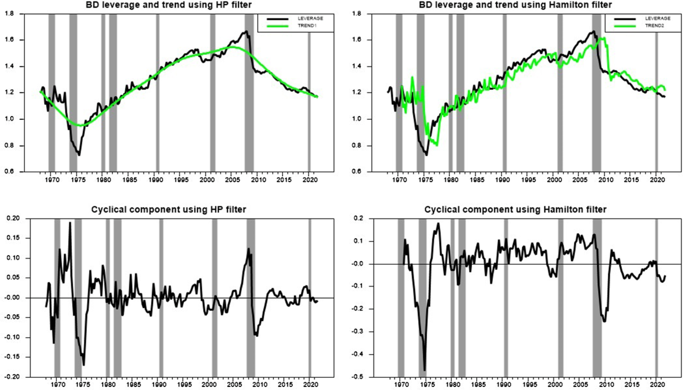
Figure 1. BD leverage and its decomposition into trended and cyclical series. The two top graphs plot BD leverage (black lines) and its trend (neon green lines) using both the HP filter (on the left) and Hamilton’s regression filter (on the right). The two bottom graphs plot the respective cyclical components of the BD leverage series, while the shaded regions show the NBER recession dates.
Another interesting feature of the raw BD leverage data is that when leverage gets far above the trend, there is often a sudden snap back toward the trend. Adrian and Shin (Reference Adrian and Shin2014) provided evidence that this sharp fall in leverage reflects the downward adjustments of the BDs balance sheets due to the high VaR. Since the BDs’ balance sheets are continuously marked to market, their responses to asset prices can be interpreted as follows. For leverage values below the trend, equity is relatively high, or VaR is relatively low, implying that BDs have some capacity to borrow through the “risk-taking channel” of monetary policy as described in Borio and Zhu (Reference Borio and Zhu2012) and Bruno and Shin (Reference Bruno and Shin2015). With the excess capacity, BDs expand their balance sheets by borrowing short-term from the REPO (repurchase agreements) market (Adrian and Shin, Reference Adrian and Shin2010). On the other hand, BDs’ VaR is relatively high when leverage is above the trend, which is defined as a situation when the value of assets relative to equity is higher than the average level. Adrian and Shin (Reference Adrian and Shin2010, Reference Adrian and Shin2014) show that in order to minimize the exposure to risks, BDs reduce their leverage by selling assets and bringing it back to desired values. Thus, the distinction between above-trend leverage and below-trend leverage is important and we use this in defining our state variable below. We will often use the notation A to denote above-trend leverage and B to denote below-trend leverage states.Footnote 16
Now compare the HP trend and the Hamilton trend by looking between the two upper row graphs in Figure 1. These graphs show that the HP trend is quite smooth, while the Hamilton trend is very jagged. The jaggedness of the Hamilton trend is not surprising because this method is designed mostly for the recovery of the cyclical part of a series. Another way to understand this is to note that the Hamilton approach runs a regression of a several step ahead value of the series on current and several lags of the series to generate the trend series. Because the current and lagged values are different at each date, the fitted value, i.e. the trend, is jagged. This is in contrast to the HP approach which uses the entire series to arrive at the trend value. As noted, we used the recommendation in Hamilton (Reference Hamilton2018) of running a regression of eight quarter ahead future values of BD leverage on current and the next three lagged values. If one were to increase the number of lags in the regression, a less jagged trend would be found. However, adding more lags also reduces the number of final detrended values as can also be seen in the plots where the Hamilton method results in both trends and detrended series that start 11 quarters later than the HP series.
The lower two graphs of Figure 1 show the cyclical values of BD leverage for each of these methods. As one would expect, these series are very similar to each other. However, there are some differences. The HP method results in about 52% of the observations being above the trend while the Hamilton method results in about 60% being above trend. Overall, the two methods are in agreement about being above and below trend 66% of the time with most of the disagreements arising around switching points from periods above trend to below trend and vice versa. As one might expect, the HP method with all its persistence built into the structure tends to have greater persistence within a state, while the Hamilton filter results in faster transitions from one state to the next.
With this intuition in mind, we define the threshold dummy variable for both the HP filter and the Hamilton approach, $I_{t-1}$
, by
$I_{t-1}$
, by
 \begin{equation} I_{t-1} = \begin{cases} 1 & \text{Leverage is above the trend,} \\ \\[-7pt] 0 & \text{Leverage is below the trend.} \end{cases} \end{equation}
As a robustness investigation, described later in the robustness section, we considered some alternative filtering assumptions. For instance, following the credit cycle literature, we choose a high smoothing parameter for the HP detrending because credit cycles are twice as long as business cycles.Footnote 17 Moreover, we also detrended the leverage series using the Baxter and King (Reference Baxter and King1999) bandpass filter, where we isolate frequencies between 4 and 64 quarters and between 8 and 32 quarters that are consistent, respectively, with credit cycle frequencies and the business cycle frequencies. The qualitative results do not change when using these alternative assumptions because the differences do not yield very different turning points. This is because our estimation technique relies on a dummy variable approach in defining the state of the economy. Hence, these differences in filtering assumptions do not yield very different turning points.
3. Data
In the baseline analysis, we use quarterly data from 1968:Q1 to 2021:Q4.Footnote 18 One potential concern for the two-sided HP filter with the full sample is the “well-known” endpoint problem. One of the many robustness checks discussed below uses an alternative sample to ensure that the endpoint problem does not pose an issue. For this check, we followed Alpanda and Zubairy (Reference Alpanda and Zubairy2019) by excluding twelve quarters from both the start and end of the sample. Another problem is that the FFR was stuck at the zero lower bound (ZLB) during the periods from 2008:Q4 to 2015:Q4 and from 2020:Q2 to 2021:Q4. Although we could drop the ZLB period data, excluding this period would greatly reduce the sample size. Furthermore, while the ZLB period raises the question of the efficacy of monetary policy during this period, Swanson and Williams (Reference Swanson and Williams2014) show that monetary policy remained effective in influencing the long-term interest rate throughout the ZLB period. In addition, other research shows that the Federal Reserve Bank’s announcements affect asset prices through their effects on financial market expectations of future monetary policy, rather than changes in the current FFR (Gürkaynak et al. Reference Gürkaynak, Sack and Swanson2005). To overcome the nearly zero values observations in the FFR during the ZLB period, we use the shadow FFR constructed by Wu and Xia (Reference Wu and Xia2016). However, as another robustness check, we show that the results are similar if we end the data interval at 2008:Q3, thus excluding the ZLB period.
Our baseline model has five variables. These include the three variables typically found in New Keynesian models, including an output measurement, an inflation measurement and a monetary policy variable. Here, we use the growth rate of real GDP (GDPC1) as our output variable. The inflation rate was computed from the consumer price index for all urban consumers (CPIAUCSL) compiled by the U.S. Bureau of Labor Statistics and the effective federal funds rate (FEDFUNDS) came from the Board of Governors of the Federal Reserve System. These data were obtained from the Federal Reserve Bank of St. Louis (FRED) database. The Wu and Xia shadow rate for the ZLB period was obtained from the Federal Reserve Bank of Atlanta. To these three variables, we add the growth rate of the BD leverage statistic described above and the VIX index. The VIX index, which is available only from 1990:Q1 onward, was obtained from the Chicago Board Options Exchange. For the pre-1990 period, we use the volatility index constructed by Bloom (Reference Bloom2009).Footnote 19 Finally, we consider several alternative economic specifications and variables for robustness checks.
4. Results
We present the baseline results in two subsections, with the first subsection focusing on the IRFs and the second focusing on the FEVD results. A third subsection describes various robustness experiments. Detailed results for the robustness experiments are available in an online appendix.
4.1 Impulse response results
We focus on the IRFs resulting from a monetary policy shock because our interest is in the monetary policy transmission mechanism and how the state of BD leverage may influence this mechanism. These IRFs are based on a one standard deviation monetary policy impulse. The identification scheme used here, in part, reflects the standard monetary policy ordering used in the literature with real GDP ordered before inflation and the FFR, which means that output can have a contemporaneous effect on inflation and the FFR. Inflation is ordered prior to the FFR, which means that inflation can have a contemporaneous effect on the FFR. Furthermore, ordering the FFR after real GDP and inflation implies that the FFR can respond to these economic variables contemporaneously.
Additionally, the ordering for BD leverage and the VIX index reflect the following considerations. We put BD leverage after real GDP and inflation to reflect that economic conditions can affect BDs’ leverage decisions contemporaneously, but not the reverse. We also put BD leverage prior to the FFR to reflect that BDs’ financial decisions can affect the FFR contemporaneously. This ordering between BD leverage and the FFR is consistent with Istiak and Serletis (Reference Istiak and Serletis2017). However, one cannot rule out that the ordering between BD leverage and the FFR could be the opposite. We reverse this ordering for these two variables in the robustness section to see if it impacts the results. Finally, following Bekaert et al. (Reference Bekaert, Hoerova and Duca2013), we order the VIX index last as changes in economic and financial conditions are more likely to affect the VIX index contemporaneously, but any changes in risk and uncertainty in the financial market should affect the economy with lags. As an additional robustness check, we also consider an alternative ordering by putting the VIX index first, followed by real GDP, inflation, BD leverage, and the interest rate.
Figure 2 shows the IRFs for three different models organized into three horizontal panels, with the top panel showing the impulse responses for a monetary shock in the linear model (1), while the next two panels show the impulse responses for the two switching models. The middle panel shows the responses when the leverage state is defined by (7) using the HP filter, while the bottom panel shows the responses when the leverage state is defined using the Hamilton filter. All three models use four lags in the forecast equations to generate IRFs, as this lag length was found optimal according to the Akaike Information Criterion (AIC).
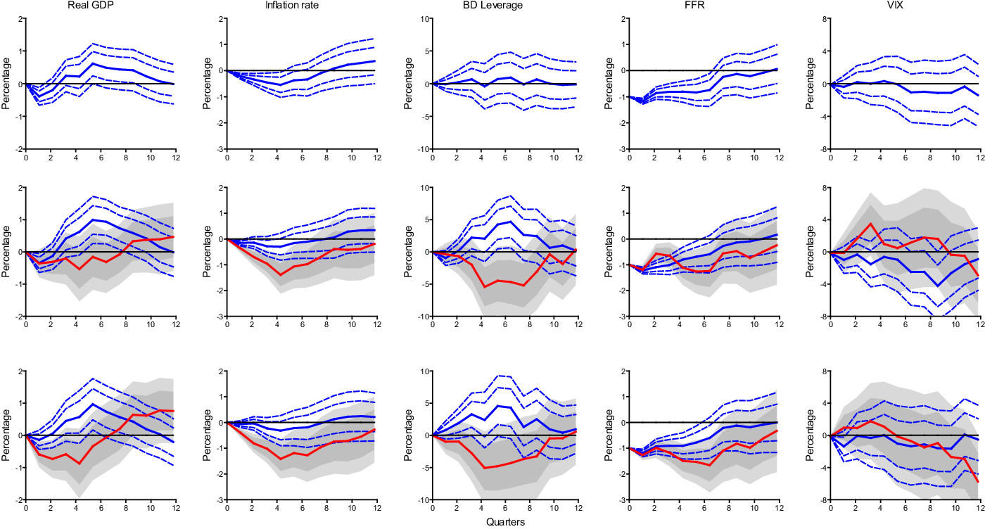
Figure 2. IRFs to a one standard deviation monetary policy shock. The top horizontal row shows the IRFs for the linear model. The second and third horizontal rows show the IRFs for the threshold models using the HP filter detrended leverage series to define the state variable in row two and the Hamilton filter detrended leverage series to define the state variable in row three. Blue solid lines show IRFs of the linear model and the below-trend leverage state of the threshold models. Dashed blue lines are 68% (inner) and 90% (outer) confidence bands around the IRFs for the linear model and the below-trend leverage state threshold models. Red solid lines show IRFs for the above-trend leverage state of the threshold models and dark and light shaded regions are 68% (dark shade) and 90% (light shade) confidence bands around these IRFs.
We use several conventions to denote various features in the different plots. In all three panels, solid lines indicate IRFs, with blue lines showing IRFs in the linear model and the below-trend state for the two state-dependent models, while red lines show the IRFs in the above-trend state for the two state-dependent models. Dashed lines represent confidence bands around some IRFs while shaded areas represent confidence bands around other IRFs. All figures include $68\%$
and
$68\%$
and $90\%$
confidence bands, which are commonly used in the monetary policy literature. For the linear models, dashed confidence bands are used and the two types are easily distinguished by their proximity to the IRF. In the switching models, two distinct conventions are used. Inner and outer confidence bands are denoted by dashed lines for the below-trend leverage state (
$90\%$
confidence bands, which are commonly used in the monetary policy literature. For the linear models, dashed confidence bands are used and the two types are easily distinguished by their proximity to the IRF. In the switching models, two distinct conventions are used. Inner and outer confidence bands are denoted by dashed lines for the below-trend leverage state ( $I_{t-1}=0$
), while dark and light shaded regions are used to distinguish
$I_{t-1}=0$
), while dark and light shaded regions are used to distinguish $68\%$
and
$68\%$
and $90\%$
confidence bands, respectively, for the above-trend leverage state (
$90\%$
confidence bands, respectively, for the above-trend leverage state ( $I_{t-1}=1$
).
$I_{t-1}=1$
).
To understand the results, we begin by focusing on the linear model in the top row. This panel shows that the output growth rate response to a one percent cut in the FFR follows a traditional hump-shaped response function.Footnote 20 It takes three quarters before the real GDP growth rate becomes positive and the increase lasts for eleven quarters. For inflation, there is a long lag before it becomes positive, requiring ten quarters for this process to play out. The initial decline in the inflation rate is well-known and was first discussed by Sims (Reference Sims1986). It is often referred to as the price puzzle. Finally, the linear model shows that there is no effect on BD leverage and the VIX from the FFR cut.
Next, we turn to the state-dependent model in the middle panel which uses the HP filter to construct the threshold structure. Let us begin by focusing on just output and inflation. A quick glance at the figures shows quite different IRFs between the two states. For the below-trend leverage state (solid blue lines with dashed confidence bands), the IRFs are quite similar to those of the linear model in the top panel. Here, the monetary stimulus results in a hump-shaped impact on output growth with a delay of three quarters and now lasting twelve quarters. The hump shape in output is larger, reaching almost one percentage point at its peak of five quarters, and is more significant over most of the path. For the below-trend state, inflation also follows a path similar to the linear model, with an initial decline that becomes positive at eight quarters. Furthermore, the initial decline is less significant than in the linear model. For the above-trend leverage state (solid red lines with shaded confidence bands), the monetary stimulus takes much longer to generate positive output growth, taking eight quarters until output growth becomes positive. Furthermore, the output growth rate never becomes significantly positive over the entire 12 quarter period. In addition, in the above-trend leverage state, the monetary policy shock induces even lower inflation, which, based on the 68% confidence band, is significantly negative for eight quarters and is never positive over the entire 12 quarter plot. The insignificant inflation rate during the below-trend leverage state, coupled with the significant negative inflation during the above-trend leverage state, shows that the price puzzle could be linked to the leverage state.
Now focus on the effects of BD leverage and the VIX. In contrast to the linear model, the responses of BD leverage to monetary stimulus differ significantly from each other between the two states. BD leverage rises significantly during the below-trend leverage state, while it falls significantly in the above-trend leverage state. The linear model masks these different responses by treating both states as the same, thus producing no change. Furthermore, the VIX mostly falls, although not significantly, during the below-trend state while it rises, significantly for four quarters, during the above-trend state. These differences in BD leverage and the VIX highlight the underlying differences between the two states. During the below-trend leverage state, the monetary stimulus can be viewed as increasing liquidity, generating economic growth, and creating bubbles in the financial markets. Since the BDs’ VaR is low in this state, they take advantage of the expansionary monetary policy by increasing leverage and building assets. The BDs’ actions cause the asset prices to rise, which in turn decreases the VIX. Alternatively, during the above-trend leverage, leverage can be viewed as too high; uninsured financial intermediaries supplying credit to BDs worry about the rising VaR and curtail credit, forcing BDs to adjust their balance sheets by selling risky assets. It leads to falling asset prices and rising uncertainty in financial markets, as is indicated by the rising responses of the VIX index.
Next, turning to the state-dependent model in the bottom panel which uses the Hamilton filter to obtain the threshold structure, we see that the IRFs are nearly identical to those generated from the HP filter, and thus the same descriptions and intuition described above hold. These similarities arise despite the fact that the overlap between the two filtering methods is only 66%. This shows that the detrending method is not important for the conclusions drawn here. The two methods result in enough commonality that they both show the same outcomes.
Overall, our results show that monetary policy shocks pass through asymmetrically and depend on the state of the leverage cycle. Monetary policy is less effective in expanding output during the above-trend leverage state. This result could be economically interpreted using insights presented in the literature. For instance, it is well established that BDs build their leverage by exploiting the advantages of low-interest rates by borrowing in the REPO market [Adrian and Shin (Reference Adrian and Shin2010), Gorton and Metrick (Reference Gorton and Metrick2012)]. This intuition works well during the below-trend leverage state. However, when leverage is already high, it triggers a collateral constraint, as noted by Mendoza (Reference Mendoza2010). BDs are forced to adjust their balance sheets by selling risky assets. As a result, this constraint causes a Fisherian deflation, which reduces the price of collateral assets. The falling asset prices and equity tighten borrowing from the money market. It also tightens unsecured lending because counterparty risks increase amidst the volatility. Intuitively, when the counterparty risks increase, the interest rate in the unsecured lending market rises. In this situation, a policy rate cut widens the interest rate spread, which we discuss in Section 5, tightening the overall credit supply in the economy. Output and factor allocations fall because access to working capital financing becomes limited. Thus, the effectiveness of expansionary monetary policy through the aggregate demand channel is curtailed in the above-trend leverage state. Recognition of this by monetary policymakers may help them undertake better monetary interventions. When leverage is low, conventional intuition about policy interventions is correct. However, when leverage is high, conventional policy intuition no longer holds, and a more nuanced policy may be needed to prevent rapid deleveraging. Because monetary policy behaves so differently during the above-trend state, policymakers may want to avoid that state by taking preemptive policy actions as leverage approaches the trend leverage threshold.
4.2 FEVD analysis
The FEVDs can also provide important insights into the asymmetric transmission of monetary policy shocks. We begin this section with a short description of how to compute FEVDs when using the linear projection methods used in this paper.Footnote 21
First, note that mean squared error of the forecast error in (1) is given by
 \begin{equation} MSE_{u}(E(x_{t+s}|X_{t}))=E(u_{t+s}^{s}u_{t+s}^{s^{\prime}})\ \ \ \ \ \ \ \ \ \ s=0,1,\ldots,h. \end{equation}
This can be estimated by using $\widehat{\sum }_{u^{s}}=\frac{1}{T}\sum _{t=1}^{T}\widehat{u}_{t+s}^{s}\widehat{u}_{t+s}^{s^{\prime}}$
, where
$\widehat{\sum }_{u^{s}}=\frac{1}{T}\sum _{t=1}^{T}\widehat{u}_{t+s}^{s}\widehat{u}_{t+s}^{s^{\prime}}$
, where $\widehat{u}_{t+s}^{s}= x_{t+s}-\widehat{\alpha }^{s}-\sum _{{i=1}}^{p}\widehat{\Gamma }_{i}^{s+1}x_{t-i}$
. The diagonal elements are the variance of the
$\widehat{u}_{t+s}^{s}= x_{t+s}-\widehat{\alpha }^{s}-\sum _{{i=1}}^{p}\widehat{\Gamma }_{i}^{s+1}x_{t-i}$
. The diagonal elements are the variance of the $s$
step ahead forecast errors for each of the elements in
$s$
step ahead forecast errors for each of the elements in $x_{t}$
. Next, we define the
$x_{t}$
. Next, we define the $n\times n$
experimental choice matrix
$n\times n$
experimental choice matrix $Q$
by the columns
$Q$
by the columns $q_{i}$
from the mapping described in (3). Renormalizing
$q_{i}$
from the mapping described in (3). Renormalizing $MSE_{u}$
by the choice matrix
$MSE_{u}$
by the choice matrix $Q$
gives
$Q$
gives
 \begin{equation} MSE_{u}(E(x_{t+s}|X_{t}))=Q^{-1}E(u_{t+s}^{s}u_{t+s}^{s^{\prime}})Q^{'-1} = Q^{-1}\sum _{u^s}Q^{'-1}\ \ \ \ \ \ s=0,1,\ldots,h. \end{equation}
From (9), we can calculate the traditional variance decompositions by directly plugging in the sample-based equivalents from the projections in (1). Extensions of this calculation to the threshold models can be done using a straightforward extension of the vector $x_{t}$
by putting
$x_{t}$
by putting $I_{t-1}x_{t}$
terms in the upper half of the new vector and
$I_{t-1}x_{t}$
terms in the upper half of the new vector and $(1-I_{t-1})x_{t}$
terms in the lower half of the new vector.
$(1-I_{t-1})x_{t}$
terms in the lower half of the new vector.
Table 1 reports the results for the 1-year and 3-year ahead FEVDs for the linear model and the two threshold models. The table only reports the results for the percent of the total forecast error variance attributable to monetary policy shocks since this is our primary interest. The table is organized into two horizontal panels, each of which corresponds to a different forecast horizon, with the top panel showing the FEVD for the 1-year forecast horizon and the bottom panel showing the FEVD for the 3-year forecast horizon. Each of the horizontal panels is also organized into five rows. The first row shows the results for the linear model given by (1), while the next two rows show the results for the threshold model given by (4) that uses the HP detrended BD leverage as the threshold indicator, and the last two rows show the results for the threshold model that uses the Hamilton detrended BD leverage as the threshold indicator. For each of the threshold models, the first row reports the FEVD above the trend and the second row reports the FEVD below the trend.
Table 1. FEVD attributable to monetary shock innovations
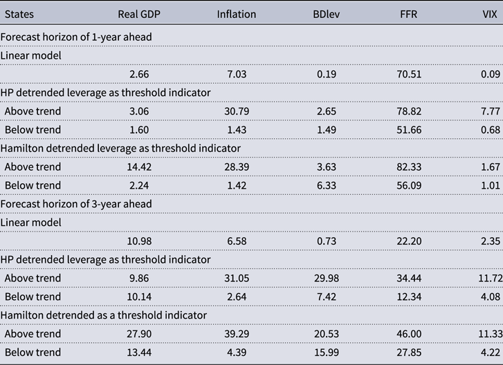
The FEVD results are mostly consistent with the IRF results. Overall, they show that monetary policy shocks have asymmetric effects that depend on the state of BD leverage. They mostly show that the percentage of the variation explained by monetary policy shocks is larger in the above-trend state with the only exceptions being the HP detrended output variation results at the 3-year horizon and the Hamilton detrended BD leverage variation results at the 1-year horizon. These higher percentages of the variation attributed to monetary policy during the above-trend leverage states likely arise because of the negative consequences seen in the IRFs for BD leverage. As noted earlier, those IRFs were consistent with BDs trying to control VaR during the above-trend leverage state and unwinding leverage. This unwinding of leverage likely spills over into the economy resulting in falling output and a larger decline in inflation. These adjustments in the above-trend leverage state result in a greater amount of variation being explained by the monetary policy stimulus. This connection between credit risks and the unwinding of BD portfolios can also be seen from the results in Section 5, where we further show that in above-trend leverage states, the credit risks in the financial markets are not pacified despite the monetary policy easing, and this likely prompts BDs to respond aggressively by unwinding their portfolios.
4.3 Robustness checks
The IRF and FEVD analysis show that the transmission of monetary policy shocks is asymmetric over the BD leverage cycle. In this subsection, we discuss various alternative specifications to check the robustness of our baseline findings. These robustness checks include (i) a three-variable model, (ii) three models with alternative monetary policy shocks, (iii) alternative filtering assumptions for the state variable, (iv) alternative Cholesky orderings, (v) alternative sample sizes, (vi) alternative economic specifications of the baseline model using other macroeconomic and financial variables and, (vii) two alternative business cycle measures, an alternative price index and lag length. Most of these robustness checks make use of modifications to the five-variable baseline model described above. However, we include a three-variable model as a check against endogeneity issues for the state variable. As noted in Gonçalves et al. (Reference Gonçalves, Herrera, Kilian and Pesavento2022), there is concern about consistency, or bias, in local projection (LP) state-dependent models. Among several sufficient conditions for consistency is to have the state depend on an exogenous variable to the model. The three variable model satisfies this condition and because the results in this model are similar to the five variable baseline model, this shows that consistency is not a concern here. The results for all of these exercises are available in an online appendix.
4.3.1 Three variable model
For the three-variable model, we use the same indicator specifications described above where the BD leverage trend defines the state variable. However, for this model, we remove the BD leverage series and the VIX index from our baseline model.Footnote 22 This means that the state variable is exogenous to the model variables and as shown in Gonçalves et al. (Reference Gonçalves, Herrera, Kilian and Pesavento2022), there is consistency in the LPs. This model, reported in Figure A.1 of the online appendix, resulted in qualitatively the same results as seen in the five-variable model providing comfort that consistency is not a concern here. Here, we see that expansionary monetary policy behaves in a conventional way during below-trend leverage states, but differs during above-trend leverage states.
4.3.2 Alternative monetary policy shocks
The second set of robustness exercises considers three alternative monetary policy shock series. Two are Divisa monetary policy aggregates, Divisa M3 and Divisa M4, advocated by Barnett (Reference Barnett1980) and Barnett et al. (Reference Barnett, Fisher and Serletis1992), and the third is the monetary policy shock sequence suggested by Romer and Romer (Reference Romer and Romer2004) using a narrative approach.Footnote 23 Dery and Serletis (Reference Dery and Serletis2021) also investigated the Divisa monetary aggregates and found that they have many desirable properties while the narrative-based monetary series has become a popular monetary policy series. In our application, we use an updated version of Romer and Romer’s monetary policy shocks reported in Coibion et al. (Reference Coibion, Gorodnichenko, Kueng and Silvia2017).Footnote 24
Figures A.2, A.3 and A.4 of the online appendix report the results for these alternative monetary policy shocks. All are versions of the five-variable baseline model. With these specifications, the impulse response dynamics are qualitatively similar to the baseline results, showing that an expansionary monetary policy shock is not effective in stimulating output in the above-trend leverage state.
4.3.3 Alternative filtering assumptions and state variable definitions
We also considered several alternative methods for filtering the leverage series to construct the threshold structure. First, we considered the alternative HP filter smoothing parameter $\lambda = 10^6$
. This choice is motivated by Bernardini and Peersman (Reference Bernardini and Peersman2018), who recommend a high smoothing parameter for HP detrending because credit cycles are twice as long as business cycles. Next, we considered the Baxter and King (Reference Baxter and King1999) band-pass filter. With this filter, we undertook exercises that isolate frequencies between 4 and 64 quarters as well as between 8 and 32 quarters, where the 4 to 64 quarter specification reflects the idea that credit cycle frequencies are twice as large as business cycle frequencies, while the 8 to 32 quarter specification matches the business cycle literature. Figure A.5 plots the cyclical components of the leverage series obtained from these alternative filtering assumptions along with the HP filter with
$\lambda = 10^6$
. This choice is motivated by Bernardini and Peersman (Reference Bernardini and Peersman2018), who recommend a high smoothing parameter for HP detrending because credit cycles are twice as long as business cycles. Next, we considered the Baxter and King (Reference Baxter and King1999) band-pass filter. With this filter, we undertook exercises that isolate frequencies between 4 and 64 quarters as well as between 8 and 32 quarters, where the 4 to 64 quarter specification reflects the idea that credit cycle frequencies are twice as large as business cycle frequencies, while the 8 to 32 quarter specification matches the business cycle literature. Figure A.5 plots the cyclical components of the leverage series obtained from these alternative filtering assumptions along with the HP filter with $\lambda = 1600$
for comparison. This figure shows similarities among the different options. We find that cyclical components using the band-pass filtering methodology are similar to those of the HP filter with
$\lambda = 1600$
for comparison. This figure shows similarities among the different options. We find that cyclical components using the band-pass filtering methodology are similar to those of the HP filter with $\lambda = 1600$
. Nevertheless, we find somewhat wider fluctuations of the cyclical components when adding a high smoothing parameter in the HP filter. In addition, we estimate a model using a truncated series of HP detrended leverage as a threshold indicator with setting
$\lambda = 1600$
. Nevertheless, we find somewhat wider fluctuations of the cyclical components when adding a high smoothing parameter in the HP filter. In addition, we estimate a model using a truncated series of HP detrended leverage as a threshold indicator with setting $\lambda = 1600$
. This is to address the well-known endpoint problem of the two-sided HP filter. Here, we excluded 12 quarters from the start and the end of the baseline sample and use a sample of 1971:Q1 to 2018:Q4. The differing filter assumptions are provided in Figure A.6, while results of the truncated series of HP detrended leverage as a threshold indicator are provided in Figure A.7. These impulse responses are similar to baseline results in Figure 2 and show that expansionary monetary policy has significant positive effects on real GDP when BD leverage is below the trend but negative or insignificant effects on real GDP when the BD leverage is above the trend.
$\lambda = 1600$
. This is to address the well-known endpoint problem of the two-sided HP filter. Here, we excluded 12 quarters from the start and the end of the baseline sample and use a sample of 1971:Q1 to 2018:Q4. The differing filter assumptions are provided in Figure A.6, while results of the truncated series of HP detrended leverage as a threshold indicator are provided in Figure A.7. These impulse responses are similar to baseline results in Figure 2 and show that expansionary monetary policy has significant positive effects on real GDP when BD leverage is below the trend but negative or insignificant effects on real GDP when the BD leverage is above the trend.
4.3.4 Alternative samples
One potential concern is that the ZLB for the FFR during the Great Recession and its aftermath, and the COVID-19 period of 2020–2021 could impact our results. To address this concern, a sub-sample ending in 2008:Q3 is considered.Footnote 25 Figure A.8 shows IRFs that are generated from this sub-sample for both of the baseline indicator series. These results are consistent with those from the baseline analysis. That is, the transmission of monetary policy is asymmetric across the states of the leverage cycle, confirming that a policy rate cut is more effective when the BD leverage is below the trend but has negative or insignificant effects when the leverage is above the trend.
4.3.5 Alternative variable orderings to identify monetary policy shocks
In the baseline model, to identify the monetary policy shocks, the VIX index is ordered last using the assumption that risk and uncertainty respond contemporaneously to monetary policy shocks [Bekaert et al. (Reference Bekaert, Hoerova and Duca2013)]. However, the VIX index does contain important information about uncertainty for future fundamentals that may have contemporaneous effects on current economic decisions.Footnote 26 In such a case, it could be argued that the VIX index should be ordered first. Hence, to identify monetary policy shocks, we consider an alternative Cholesky ordering which puts the VIX index first, followed by output, inflation, BD leverage, and the FFR. Another reasonable ordering follows from Bruno and Shin (Reference Bruno and Shin2015). They show that BDs contemporaneously respond to changes in monetary policy. Based on these results, the FFR should be ordered before BD leverage. Under these alternative orderings, seen in Figures A.9 and A.10, we find that looser monetary policy in the above-trend leverage state is not stimulative for economic or financial variables.
4.3.6 Alternative economic specifications
Here, we consider several alternative economic specifications to measure economic activities and investigate how they respond to an expansionary monetary shock between the two states of the economy. In the first model, we consider nondurable and durable goods consumption along with BD leverage, the FFR, and the VIX index. In another, we include real investment, credit to the private sector, and housing prices along with the output and the interest rate. We also experimented with alternative ordering within these alternative economic specifications. For instance, in one specification, we ordered the FFR after the credit to the private sector, while in another specification, we reversed the order. In these alternative specifications, we excluded the inflation rate, and following Bekaert et al. (Reference Bekaert, Hoerova and Duca2013), we consider the real interest rate (the FFR minus inflation) as a measure of the monetary policy stance. The IRFs using these three alternative specifications (seen in Figures A.11, A.12 and A.13) again show significant differences in response of economic activities to monetary policy shocks which depend on whether leverage is below or above trend.
4.3.7 Alternative output and price index measurements as well as lag lengths
Additionally, we consider four other alternative specifications of our baseline model which investigated different output and price index measurements and lag lengths. These include replacing real GDP with industrial production and the output gap. In another, we consider an alternative measure of inflation by swapping the inflation rate computed from the consumer price index for all urban consumers with an inflation rate computed from the personal consumption index. Finally, we consider an alternative lag length model using two lags based on the Bayesian Information Criterion (BIC). These alternative data series and lag length specifications, seen in Figures A.14, A.15, A.16, and A.17, resulted in the same qualitative results, showing that monetary policy impact during the below-trend leverage periods was similar to those of the linear model, while in above-trend leverage periods, expansionary monetary policy effects look similar to those of traditional contractionary monetary policy.
5. Monetary policy and credit risk
Heretofore the focus has been on what the IRFs and FEVD tell us about the monetary policy effects on economic variables across the leverage cycle. We have seen evidence that the monetary policy transmission mechanism changes depending on the state of the leverage cycle and that during above-trend leverage states, BDs reduce their leverage, which is associated with a rising VIX index in response to expansionary monetary policy and may, in part, explain why stimulative monetary policy is less effective during this phase of the leverage cycle. In this section, we provide further evidence of the strains on BDs by looking at interest rates that BDs are routinely involved with. Here, we focus on the TED spread, which is defined as the difference between the yield on 3-month London Interbank Offered Rate loans (LIBOR) and the U.S. 3-month Treasury rate.Footnote 27 BDs are routine participants in the LIBOR market and an increase in the TED spread is one of the most commonly followed measures of funding conditions that financial intermediaries take into consideration when they decide on their risk exposure.Footnote 28 In normal times, the TED spread is very small, and money flows freely and cheaply between banks because of low default risks.Footnote 29 However, in bad times, the interbank loan rate (LIBOR) rises as banks demand more interest to make up for the rising risk of default. Therefore, a lower TED spread reflects higher liquidity in the market, while a higher spread indicates less willingness to lend by major banks. Here, we show that the TED spread and hence the transmission mechanism of monetary policy depends on the state of BD leverage.Footnote 30
We investigate these connections using a threshold regression model given by
 \begin{equation} TED \ Spread_{t}=I_{t-1}\Bigg [\alpha ^{A}+\sum _{i=0}^n\beta _i^{A}\Delta FFR_{t-i}\Bigg ]+(1-I_{t-1})\Bigg [\alpha ^{B}+\sum _{i=0}^n\beta _i^{B}\Delta FFR_{t-i}\Bigg ]+\nu _{t}, \end{equation}
where $\alpha ^{j}$
and
$\alpha ^{j}$
and $\beta _i^{j}$
are constant and coefficient notations, respectively, and the index
$\beta _i^{j}$
are constant and coefficient notations, respectively, and the index $i=0,\ldots n$
is used to indicate lags for the independent variables. We investigate models that have
$i=0,\ldots n$
is used to indicate lags for the independent variables. We investigate models that have $n=0,\ldots 4$
lags. In addition, we use the index
$n=0,\ldots 4$
lags. In addition, we use the index $j\in \{A,B\}$
to distinguish above and below-trend leverage states. Changes in the stance of monetary policy are measured by
$j\in \{A,B\}$
to distinguish above and below-trend leverage states. Changes in the stance of monetary policy are measured by $\Delta FFR_{t}$
where for date
$\Delta FFR_{t}$
where for date $t$
,
$t$
, $\Delta FFR_{t}$
is the difference between FFR at quarter
$\Delta FFR_{t}$
is the difference between FFR at quarter $t$
and quarter
$t$
and quarter $t-1$
, and
$t-1$
, and $\nu _{t}$
is the error term. The indicator series
$\nu _{t}$
is the error term. The indicator series $I_{t-1}\in \{0,1\}$
are defined as before by using (7), and either the HP filter or the Hamilton filter is used to determine whether BD leverage is above or below trend. For comparison purposes, we also estimate a linear version of (10) which does not include the switching structure. The regressions are run using data from 1986:Q1 to 2021:Q4, and the data for the
$I_{t-1}\in \{0,1\}$
are defined as before by using (7), and either the HP filter or the Hamilton filter is used to determine whether BD leverage is above or below trend. For comparison purposes, we also estimate a linear version of (10) which does not include the switching structure. The regressions are run using data from 1986:Q1 to 2021:Q4, and the data for the $TED \ Spread$
(TEDRATE) is obtained from the FRED website. This data interval starts somewhat later than IRF and FEVD analysis because the TED spread data is not available prior to 1986:Q1.
$TED \ Spread$
(TEDRATE) is obtained from the FRED website. This data interval starts somewhat later than IRF and FEVD analysis because the TED spread data is not available prior to 1986:Q1.
Table 2 shows the results of these exercises. The table is organized into three vertical panels, where the first panel shows the results for various linear models which do not distinguish the above- and below-trend leverage states, while the next two panels show various HP-filtered and Hamilton-filtered state-dependent models. For both linear- and state-dependent models, we included a range of lags, with the first model having no lags ( $n=0$
) and the next four models incrementally adding additional lags. The table is also organized into three horizontal panels with the top panel (rows beginning with “
$n=0$
) and the next four models incrementally adding additional lags. The table is also organized into three horizontal panels with the top panel (rows beginning with “ $\alpha$
or
$\alpha$
or $\alpha ^B$
” and ending with “
$\alpha ^B$
” and ending with “ $\beta _4$
or
$\beta _4$
or $\beta _4^B$
”) having either the linear model coefficient results or the below-trend leverage state coefficient results for the state-dependent models, while the middle panel (rows beginning with “
$\beta _4^B$
”) having either the linear model coefficient results or the below-trend leverage state coefficient results for the state-dependent models, while the middle panel (rows beginning with “ $\alpha ^A$
” and ending with “
$\alpha ^A$
” and ending with “ $\beta _4^A$
”) has only the above-trend leverage state coefficient results for the state-dependent models. The third horizontal panel (rows beginning with
$\beta _4^A$
”) has only the above-trend leverage state coefficient results for the state-dependent models. The third horizontal panel (rows beginning with $R^2$
and ending with the Bayesian Information Criterion which is abbreviated as
$R^2$
and ending with the Bayesian Information Criterion which is abbreviated as $BIC$
) reports common regression information, such as
$BIC$
) reports common regression information, such as $R^2$
, at the bottom of the table. All standard errors are computed using the Newey-West procedure with four lags.Footnote
31
$R^2$
, at the bottom of the table. All standard errors are computed using the Newey-West procedure with four lags.Footnote
31
Table 2. Ted spread regression results
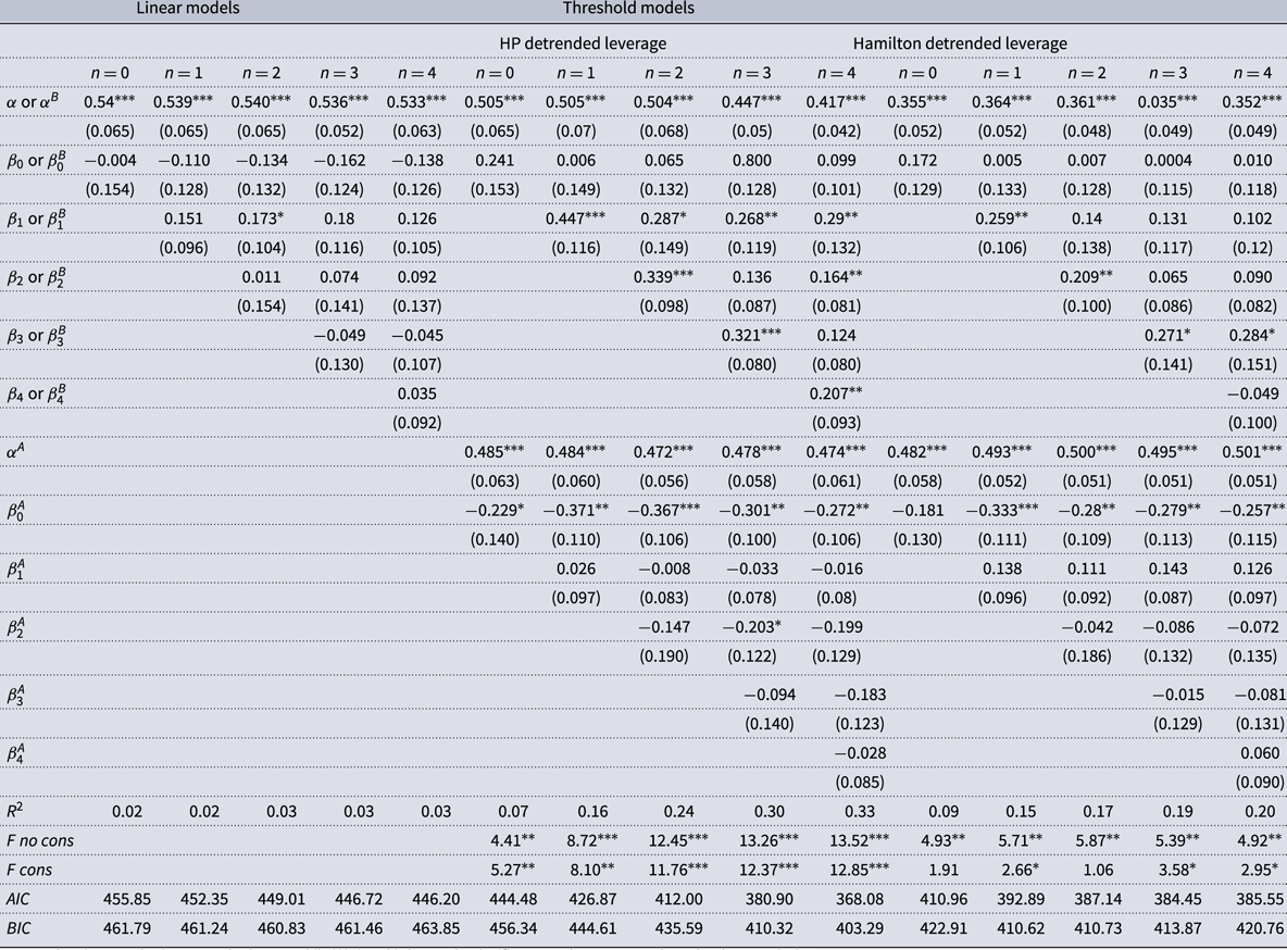
Notes: Values in parenthesis are standard errors while ***, * and * denote the significance at the 1%, 5%, and 10% level, respectively.
To interpret the results in Table 2, it is important to start by understanding how $\Delta FFR_{t}$
is computed. As noted earlier,
$\Delta FFR_{t}$
is computed. As noted earlier, $\Delta FFR_{t}$
is the difference between
$\Delta FFR_{t}$
is the difference between $FFR$
in quarter
$FFR$
in quarter $t$
and quarter
$t$
and quarter $t-1$
. This means positive values indicate contractionary monetary policy, and negative values indicate expansionary monetary policy. Because the real-world cases where highly leveraged states produced counter-intuitive economic outcomes occurred during the expansionary policy, we will use negative values for the independent variable in our discussion below.
$t-1$
. This means positive values indicate contractionary monetary policy, and negative values indicate expansionary monetary policy. Because the real-world cases where highly leveraged states produced counter-intuitive economic outcomes occurred during the expansionary policy, we will use negative values for the independent variable in our discussion below.
Looking at Table 2, note that the coefficients in the linear model are mostly insignificant, with only the first lag in the two lag model showing a marginal 10% level of significance. This is not surprising because as we will see, it is the state of the leverage cycle that is important.Footnote
32
Next, looking at the state-dependent models, we see similarities between the models using the two detrending methods. Both detrending methods show a few significant positive coefficients for the below-trend leverage states and consistently show significant negative coefficients for the no-lag coefficient in the above-trend leverage states. The positive coefficients in the below-trend leverage states mean that expansionary monetary policy, which has negative values for $\Delta FFR_{t}$
, results in TED spread decreasing. This means expansionary monetary policy can be interpreted as relieving credit stress.
$\Delta FFR_{t}$
, results in TED spread decreasing. This means expansionary monetary policy can be interpreted as relieving credit stress.
On the other hand, the negative coefficients in the above-trend leverage states mean expansionary monetary policy widens the difference between the LIBOR rate and the Treasury Bill rate, thus aggravating credit stress. This situation likely arises because financial institutions, which are nervous about lending to each other in the REPO market, demand higher collateral because of the risk of default on a loan or a higher market price (LIBOR rate) for taking on the risk. Geanakoplos (Reference Geanakoplos2010) and Gorton and Metrick (Reference Gorton and Metrick2012) show that when collateral requirements increase, leverage falls. As a result, the risk-bearing capacity of the financial system can be diminished, which eventually reinforces further withdrawal of credit and deleveraging. The credit risks can, therefore, be deemed as the empirical link between monetary policy and BDs’ decisions on leverage, which in turn, have macroeconomic implications because increasing credit risks reduce the credit supply to the real sector. Our robustness checks using alternative economic specifications of the baseline model in Section 4.3.6 show that when the leverage is above the trend, credit to the private sector and investment decline significantly following an interest rate cut (seen in Figures A.12 and A.13 in the online appendix). Finally, looking at the bottom panel of Table 2, we see that the $F$
-statistics testing equality of the coefficients in the above-trend leverage and below-trend leverage states are mostly significant, indicating the switching model is appropriate. This means that these different responses to expansionary monetary policy in the two states are important characteristics for measuring credit risk in financial markets.
$F$
-statistics testing equality of the coefficients in the above-trend leverage and below-trend leverage states are mostly significant, indicating the switching model is appropriate. This means that these different responses to expansionary monetary policy in the two states are important characteristics for measuring credit risk in financial markets.
The results from the IRFs in combination with the results from the TED spread regressions show that there are different monetary policy transmission mechanisms in the above- and below-trend leverage states. Because of the similarities of the below-trend leverage state with the single state results, it is reasonable to infer that the transmission mechanism follows a traditional path in the below-trend leverage state. In particular, lower interest rates stimulate output through the traditional aggregate demand channel where the lower interest rates encourage higher spending on investment goods. On the other hand, the above-trend leverage case is consistent with two opposing demand effects and the dynamics can be thought of in terms of the relative strengths of the two effects. First, lower interest rates stimulate demand through the traditional aggregate demand channel in which the lower interest rates encourage higher investment spending. Second, the lower interest rates induce a chain of risk issues in the REPO markets which cut aggregate demand. In particular, as seen in both the impulse response of the VIX index and the TED spread results, an interest rate cut raises risk in the REPO market which induces BD to reduce VaR by reducing borrowing, resulting in a pullback in aggregate demand. The net above-trend leverage effect is then the sum of these two opposing forces. The IRFs from the HP filter shows that there is virtually no net increase in demand from the interest rate cut. However, the IRF from the Hamilton filter paints a darker picture in that the risk channel dominates the investment spending channel and net demand actually decreases in the above-trend state. The differences in the effects of monetary policy on economic activities between the above-trend state and below-trend state are distinct when considering alternative economic specifications of the baseline model (seen in Figures A.11, A.12 and A.13 in the online appendix).
Recognizing that monetary stimulus works differently in the above-trend leverage case is important to policymakers because of the longer lag associated with monetary policy. In general, monetary policymakers know that demand stimulus from interest rate cuts take time to entice increases in investment spending, so they tend to be patient for the effects of policy to kick in. However, because of the muted or negative effects of policy in the above-trend leverage state, patience will not help if there is no net stimulus to be seen. Because policy is at best ineffective and at worst destructive in the above-trend leverage state, policymakers may wish to avoid this state by taking preemptive actions to prevent excess leverage by BD. Similar recommendations have been made by Geanakoplos (Reference Geanakoplos2010) and Smets (Reference Smets2018).
6. Conclusion
In this paper, we study the role of BD leverage in the monetary policy transmission mechanism. We use BD leverage to construct a regime-switching indicator and investigate the transmission of monetary policy across the leverage cycle in the United States. Using a state-dependent LP model of the type described by Jordà (Reference Jordà2005), we find that the monetary transmission mechanism is quite different in below-trend leverage and above-trend leverage states. Specifically, the results show that during the below-trend leverage state, expansionary monetary policy works in a traditional fashion through investment and aggregate demand stimulus. However, in the above-trend leverage state, monetary policy works through a combination of effects, including the traditional investment demand channel that is stimulative and a risk mitigation channel which is antistimulative. The net effect for expansionary monetary policy depends on the relative strengths of these opposing forces and is at best ineffective and at worst is destructive.
These findings show that monetary policymakers may need to be more thoughtful about economic conditions when they consider policy. If BD leverage is below trend, then policy will have its intended effects. However, if BD leverage is above trend, then policy will not work as desired. Because of the diminished or even opposite effect of policy in the above-trend leverage state, policymakers need to be careful when implementing policy under these conditions. Furthermore, because of the possibility of adverse policy effects in the above-trend leverage state, policymakers may wish to avoid this state by undertaking preemptive policy as BD leverage moves above its trend.
Supplementary material
To view supplementary material for this article, please visit https://doi.org/10.1017/S1365100523000081.


 Open access