


1 Introduction
The classic framework for the theoretical study of turbulent plumes and the widely adopted model that captures the streamwise variation in plume entrainment were reported in the mid-twentieth century (Priestley & Ball Reference Priestley and Ball1955; Morton, Taylor & Turner Reference Morton, Taylor and Turner1956). However, until now, analytical solutions for turbulent plumes with such variable entrainment have eluded us. In this paper, we develop these solutions, solving directly the plume conservation equations subject to a local variability in entrainment. The applicability of the solutions we provide for the mean fluxes of volume and momentum is wide, spanning forced, pure and lazy plume releases. These solutions are complemented by expressions for the location of the virtual origin and insights into the streamwise variation of the Richardson number (§ 2). The close agreement we observe between these predictions and measurements of the virtual origin inferred from experiments (§ 3) provides confidence in their practical application.
Turbulence in a buoyant plume approaches a state of local equilibrium with height (Turner Reference Turner1986). This state of equilibrium, referred to as a ‘pure’ plume (Morton Reference Morton1959), allows for straightforward mathematical descriptions of turbulent entrainment that are based on self-similarity, i.e. on parameterisations of mixing that are locally invariant. This parameterisation forms the basis for the closure of the plume conservation equations of Morton et al. (Reference Morton, Taylor and Turner1956) whose solutions have been used to predict the dynamics of turbulent plumes in nature, industry and the built environment (see the reviews by Kaye (Reference Kaye2008), Woods (Reference Woods2010) and Hunt & van den Bremer (Reference Hunt and van den Bremer2011)).
For the pure plume, a height-invariant description of entrainment has legitimately been assumed and analytical solutions to these equations widely reported (Morton Reference Morton1959; Morton & Middleton Reference Morton and Middleton1973; Hunt & Kaye Reference Hunt and Kaye2001, Reference Hunt and Kaye2005). Pure plumes do not exhibit a dynamical variability with height (Ezzamel, Salizzoni & Hunt Reference Ezzamel, Salizzoni and Hunt2015), their behaviour characterised by a local Richardson number  $Ri(z)$ which maintains the unique pure-plume source value $Ri(z)=Ri_{p}$ at all heights $z\geqslant 0$; $z$ denotes the vertical coordinate with origin coincident with the physical source and $Ri_{p}$ the (constant) pure-plume Richardson number. These solutions treat the plume as self-similar at all distances from the source; this is satisfied only when the release is ‘pure’ (Turner Reference Turner1986; Hunt & Kaye Reference Hunt and Kaye2005), beyond the near-source region of flow establishment (Fischer et al. Reference Fischer, List, Koh, Imberger and Brooks1979).
Plumes from general (i.e. non-pure plume) area sources, however, are released such that the local conditions are distinct from those that characterise the self-similar state (Turner Reference Turner1986). These plumes are in a ‘non-pure’ state, either locally ‘forced’ or ‘lazy’, and undergo an adjustment between the source and the far field (Morton Reference Morton1959; Morton & Middleton Reference Morton and Middleton1973). The buoyancy force drives this adjustment and consequently there is dynamical variability, characterised by  $Ri(z)\rightarrow Ri_{p}$, so that local conditions in the plume, including entrainment, are expected to depend on $Ri(z)$. This behaviour has been confirmed by measurements, in both thermal and aqueous-saline plumes, that show these imbalances radically change the entrainment in the proximity of the source and the approach to the self-similar state (Papanicolaou & List Reference Papanicolaou and List1988; Wang & Law Reference Wang and Law2002; Kaye & Hunt Reference Kaye and Hunt2009; Ezzamel et al. Reference Ezzamel, Salizzoni and Hunt2015). Further support for modified entrainment due to non-pure-plume behaviour has been garnered from direct numerical simulation (DNS) and theoretical studies (van Reeuwijk et al. Reference van Reeuwijk, Salizzoni, Hunt and Craske2016; Marjanovic, Taub & Balachandar Reference Marjanovic, Taub and Balachandar2017).
Studies on turbulent plumes spanning over 60 years of research are aligned in their view that entrainment for non-pure plumes varies as a linear function of the local Richardson number (Priestley & Ball Reference Priestley and Ball1955; Papanicolaou & List Reference Papanicolaou and List1988; Wang & Law Reference Wang and Law2002; Kaminski, Tait & Carazzo Reference Kaminski, Tait and Carazzo2005; Ezzamel et al. Reference Ezzamel, Salizzoni and Hunt2015; van Reeuwijk & Craske Reference van Reeuwijk and Craske2015). Beginning with Priestley & Ball (Reference Priestley and Ball1955), entrainment was modelled by invoking this form for the case of a forced plume ( $Ri(z)<Ri_{p}$), wherein a linear entrainment function $\unicode[STIX]{x1D6FC}=\unicode[STIX]{x1D6FC}(Ri(z))$ was introduced and matched between values measured for the pure jet and the pure plume. More recently, the same form for the entrainment function was deduced based on solutions of the plume conservation equations which are consistent with the equations for the conservation of energy fluxes (Kaminski et al. Reference Kaminski, Tait and Carazzo2005; van Reeuwijk & Craske Reference van Reeuwijk and Craske2015). On account of these developments placing no restrictions on the source condition for the plume, we have referred to this linear entrainment function as being universal. Surprisingly, despite the wide acceptance of this form, analytical solutions to the plume conservation equations subject to a linear dependence of the entrainment function with Richardson number have not previously been reported. Our motivation herein is therefore twofold: (i) to develop analytical solutions to the plume conservation equations for entrainment following a linear variation with local Richardson number and (ii) to determine the associated locations of the virtual origin for general forced, pure and lazy plumes from area sources.
The virtual origin refers to the location at which a point source of buoyancy flux would give rise to a plume whose behaviour matches the far-field behaviour of the actual (area source) plume of interest. In essence, the virtual origin is deduced as a vertical offset, or correction, to the analytical solutions for a plume formed from a point source of buoyancy flux. Hunt & Kaye (Reference Hunt and Kaye2001) provide a theoretical description of the origin location based on the solution to the plume equations for  $\unicode[STIX]{x1D6FC}=\text{constant}$. Whilst origin corrections are often instrumental in theoretical developments for which the plume is a single component of the overall system (Kaye & Hunt Reference Kaye and Hunt2007), the magnitude of this correction and its dependence on the source conditions have not been determined for the aforementioned linear entrainment model.
The remainder of this paper is structured as follows. In § 2 analytical solutions are derived for a plume from a point source and a general area source. We then develop expressions for the virtual origin, make comparisons with laboratory measurements (§ 3), and discuss the insights these solutions provide regarding the approach of the plume to the self-similar state. Conclusions are drawn in § 5.
2 Solutions to the plume equations
Denoting  $z$ as the vertical coordinate with origin at the physical source, the steady integral conservation equations of Morton et al. (Reference Morton, Taylor and Turner1956) for the time-averaged fluxes of volume $\unicode[STIX]{x03C0}Q$, specific momentum $\unicode[STIX]{x03C0}M$ and buoyancy $\unicode[STIX]{x03C0}B$ of an axisymmetric plume in an unstratified and otherwise quiescent environment may be expressed as
 $$\begin{eqnarray}\frac{\text{d}Q}{\text{d}z}=2\unicode[STIX]{x1D6FC}M^{1/2},\quad \frac{\text{d}M}{\text{d}z}=\unicode[STIX]{x1D705}\frac{BQ}{M},\quad \frac{\text{d}B}{\text{d}z}=0,\end{eqnarray}$$
 where  $\unicode[STIX]{x1D705}=1$ for top-hat and $\unicode[STIX]{x1D705}=2$ for Gaussian profiles of buoyancy and vertical velocity. A derivation of (2.1) is given, for example, in Hunt & van den Bremer (Reference Hunt and van den Bremer2011). Following classic plume theory, the solution to these governing equations relies on a turbulence closure, known as the entrainment hypothesis, which relates the horizontal velocity of the fluid entrained peripherally into the plume $u_{e}$ to a local vertical velocity $w$
$w$
 $$\begin{eqnarray}u_{e}:=\unicode[STIX]{x1D6FC}w.\end{eqnarray}$$
 Widely referred to as the entrainment coefficient, herein we refer to  $\unicode[STIX]{x1D6FC}$ as the entrainment function (cf. Marjanovic et al. Reference Marjanovic, Taub and Balachandar2017) as we acknowledge that $\unicode[STIX]{x1D6FC}$ may be constant or take a functional form depending on the source conditions. The assumption of a constant $\unicode[STIX]{x1D6FC}$ relies on the spatial invariance of the local turbulence as achieved when there is a specific balance of the buoyancy and inertial forces acting on the flow (Turner Reference Turner1986). Following Turner (Reference Turner1973), the ratio of these forces, whether in balance or otherwise, is characterised locally by the Richardson number
 $$\begin{eqnarray}Ri(z):=\frac{BQ^{2}(z)}{M^{5/2}(z)}.\end{eqnarray}$$
 Regardless of the conditions imposed at source, all plumes naturally tend to a pure-plume self-similar state with streamwise distance  $z$ in which the local Richardson number is invariant, i.e. $Ri(z)\rightarrow Ri_{p}=\text{constant}$ as $z\rightarrow \infty$ (Morton Reference Morton1959; Hunt & Kaye Reference Hunt and Kaye2001). It follows, from (2.1) and (2.3), that the vertical variation of the Richardson number is
 $$\begin{eqnarray}\frac{\text{d}Ri}{\text{d}z}=\left(4\unicode[STIX]{x1D6FC}Ri-\frac{5\unicode[STIX]{x1D705}}{2}Ri^{2}\right)\frac{M^{1/2}}{Q}.\end{eqnarray}$$
 Morton et al. (Reference Morton, Taylor and Turner1956) deduced power-law solutions for the fluxes  $Q$ and $M$ for the point-source plume, i.e. solving (2.1) subject to the source conditions $Q_{0}=M_{0}=0$ and $B_{0}>0$ at $z=0$. Morton (Reference Morton1959) then extended the analysis to area sources. He demonstrated that these plumes may be characterised by a scaled source Richardson number
 $$\begin{eqnarray}\unicode[STIX]{x1D6E4}_{0}:=\frac{Ri_{0}}{Ri_{p}}\quad \text{where }Ri_{0}=\frac{B_{0}Q_{0}^{2}}{M_{0}^{5/2}}.\end{eqnarray}$$
 For non-pure source conditions, i.e.  $Ri_{0}\neq Ri_{p}$, the source fluxes create an imbalance from the pure-plume state in the proximity of the source, where locally the scaled Richardson number $\unicode[STIX]{x1D6E4}(z):=Ri(z)/Ri_{p}\neq 1$. Morton (Reference Morton1959) presented approximate solutions to (2.1) for $0<\unicode[STIX]{x1D6E4}_{0}<1$ (so-called forced plumes) based on a vertical offset to the pure-plume power-law solutions; these vertical offsets being widely referred to as virtual origin corrections. Morton & Middleton (Reference Morton and Middleton1973) extended his analysis to plumes from sources for which $\unicode[STIX]{x1D6E4}_{0}>1$ (so-called lazy plumes). Hunt & Kaye (Reference Hunt and Kaye2001) subsequently deduced analytical solutions for the plume fluxes and virtual origin valid for both forced and lazy cases. The aforementioned solutions are all based on the assumption of a constant value of $\unicode[STIX]{x1D6FC}$ and thus do not take into account changes in behaviour due to imbalances from pure-plume behaviour.
2.1 The entrainment function
Non-pure plumes that are formed from area sources do not exhibit spatially invariant turbulence and are characterised by a vertical variation of the local Richardson number, from a source value of  $Ri_{0}$ to the far-field value of $Ri_{p}$ (Turner Reference Turner1986). Several analyses of the derivation of the plume conservation equations, including those of Priestley & Ball (Reference Priestley and Ball1955), Kaminski et al. (Reference Kaminski, Tait and Carazzo2005) and van Reeuwijk & Craske (Reference van Reeuwijk and Craske2015), have shown that the entrainment function takes the form
 $$\begin{eqnarray}\unicode[STIX]{x1D6FC}:=\unicode[STIX]{x1D6FE}_{1}+\unicode[STIX]{x1D6FE}_{2}Ri,\end{eqnarray}$$
 for constant coefficients  $\unicode[STIX]{x1D6FE}_{1}>0$ and
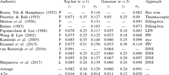
  $\unicode[STIX]{x1D6FE}_{2}>0$. Table 1 summarises historical numerical predictions and experimental measurements of these coefficients. The solution of (2.1c) is $B=B_{0}$ irrespective of the entrainment function. Carazzo, Kaminski & Tait (Reference Carazzo, Kaminski and Tait2006) propose an extended form of (2.6) that compensates for the adjustment of the cross-stream velocity and buoyancy profiles with streamwise distance (see discussion in appendix A). Invoking the entrainment function (2.6), the conservation equations (2.1a,b) become
 $$\begin{eqnarray}\frac{\text{d}Q}{\text{d}z}=2\unicode[STIX]{x1D6FE}_{1}M^{1/2}+2\unicode[STIX]{x1D6FE}_{2}B_{0}\frac{Q^{2}}{M^{2}},\quad \frac{\text{d}M}{\text{d}z}=\unicode[STIX]{x1D705}B_{0}\frac{Q}{M}.\end{eqnarray}$$
2.2 Point-source solution
For the point source,  $Q_{0}=M_{0}=0$ at $z=0$. Thus, guided by dimensional considerations, we seek the power-law solutions
 $$\begin{eqnarray}Q=C_{Q}B_{0}^{1/3}z^{5/3},\quad M=C_{M}B_{0}^{2/3}z^{4/3}.\end{eqnarray}$$
Substituting (2.8) into (2.7) yields the coefficients
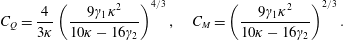 $$\begin{eqnarray}C_{Q}=\frac{4}{3\unicode[STIX]{x1D705}}\left(\frac{9\unicode[STIX]{x1D6FE}_{1}\unicode[STIX]{x1D705}^{2}}{10\unicode[STIX]{x1D705}-16\unicode[STIX]{x1D6FE}_{2}}\right)^{4/3},\quad C_{M}=\left(\frac{9\unicode[STIX]{x1D6FE}_{1}\unicode[STIX]{x1D705}^{2}}{10\unicode[STIX]{x1D705}-16\unicode[STIX]{x1D6FE}_{2}}\right)^{2/3}.\end{eqnarray}$$
Table 1. Values for  $\unicode[STIX]{x1D6FE}_{1}$ and $\unicode[STIX]{x1D6FE}_{2}$ in axisymmetric plumes. Entries for the pure-plume entrainment coefficient $\unicode[STIX]{x1D6FC}_{p}$ are given. The letters P, J, F and L are indicative of plume behaviour in each study. P indicates a pure plume, J a pure jet, F a forced plume and L a lazy plume. Hereafter, we take the average values listed. LDV (laser-Doppler velocimetry). PIV (particle image velocimetry).
2.3 Area-source solution
For the general area-source conditions  $Q_{0}>0$, $M_{0}>0$ and $B_{0}>0$, we scale $Q$ and $M$ on their respective source values and the streamwise coordinate on $L_{q}:=Q_{0}/M_{0}^{1/2}$. Thus, we introduce
 $$\begin{eqnarray}\unicode[STIX]{x1D701}:=\frac{z}{L_{q}},\quad q:=\frac{Q}{Q_{0}},\quad m:=\frac{M}{M_{0}}.\end{eqnarray}$$
 Note, for top-hat profiles,  $L_{q}$ is the radius of the source. Accordingly, (2.7) reduce to
 $$\begin{eqnarray}\frac{\text{d}q}{\text{d}\unicode[STIX]{x1D701}}=2\unicode[STIX]{x1D6FE}_{1}m^{1/2}+2\unicode[STIX]{x1D6FE}_{2}Ri_{p}\unicode[STIX]{x1D6E4}_{0}\frac{q^{2}}{m^{2}},\quad \frac{\text{d}m}{\text{d}\unicode[STIX]{x1D701}}=\unicode[STIX]{x1D705}Ri_{p}\unicode[STIX]{x1D6E4}_{0}\frac{q}{m},\end{eqnarray}$$
where the pure-plume Richardson number is given by
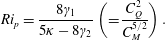 $$\begin{eqnarray}Ri_{p}=\frac{8\unicode[STIX]{x1D6FE}_{1}}{5\unicode[STIX]{x1D705}-8\unicode[STIX]{x1D6FE}_{2}}\left(=\frac{C_{Q}^{2}}{C_{M}^{5/2}}\right).\end{eqnarray}$$
Combining (2.11a) and (2.11b) gives the nonlinear differential equation
 $$\begin{eqnarray}\frac{\text{d}q}{\text{d}m}=\frac{2\unicode[STIX]{x1D6FE}_{1}}{\unicode[STIX]{x1D705}Ri_{p}\unicode[STIX]{x1D6E4}_{0}}\frac{m^{3/2}}{q}+\frac{2\unicode[STIX]{x1D6FE}_{2}}{\unicode[STIX]{x1D705}}\frac{q}{m}.\end{eqnarray}$$
 Defining  $\mathscr{A}_{1}(m):=2\unicode[STIX]{x1D6FE}_{1}m^{3/2}/\unicode[STIX]{x1D705}Ri_{p}\unicode[STIX]{x1D6E4}_{0}$ and $\mathscr{A}_{2}(m):=-2\unicode[STIX]{x1D6FE}_{2}/\unicode[STIX]{x1D705}m$, (2.13) becomes
 $$\begin{eqnarray}\frac{\text{d}q}{\text{d}m}=\mathscr{A}_{1}(m)q^{-1}-\mathscr{A}_{2}(m)q.\end{eqnarray}$$
 This is the Bernoulli differential equation for which solutions are readily available (Ince Reference Ince1956, pp. 22–23). With the change of variable  $\unicode[STIX]{x1D702}:=q^{2}$, (2.14) reduces to the linear differential equation
 $$\begin{eqnarray}\frac{\text{d}\unicode[STIX]{x1D702}}{\text{d}m}=2q\frac{\text{d}q}{\text{d}m}=A_{1}(m)-\unicode[STIX]{x1D702}A_{2}(m),\end{eqnarray}$$
 where  $A_{1}(m):=2\mathscr{A}_{1}(m)$ and $A_{2}(m):=2\mathscr{A}_{2}(m)$. Writing $c$ as a constant of integration, the solution of (2.15) is
 $$\begin{eqnarray}\unicode[STIX]{x1D702}=\frac{\displaystyle \int \exp \left(\displaystyle \int A_{2}(m)\,\text{d}m\right)A_{1}(m)\,\text{d}m+c}{\exp \left(\displaystyle \int A_{2}(m)\,\text{d}m\right)}.\end{eqnarray}$$
 Integrating from the source, where  $q=1$ and $m=1$, the solution of (2.13) is thus
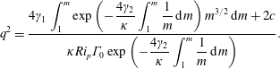 $$\begin{eqnarray}q^{2}=\frac{4\unicode[STIX]{x1D6FE}_{1}\displaystyle \int _{1}^{m}\exp \left(-{\displaystyle \frac{4\unicode[STIX]{x1D6FE}_{2}}{\unicode[STIX]{x1D705}}}\displaystyle \int _{1}^{m}{\displaystyle \frac{1}{m}}\,\text{d}m\right)m^{3/2}\,\text{d}m+2c}{\unicode[STIX]{x1D705}Ri_{p}\unicode[STIX]{x1D6E4}_{0}\exp \left(-{\displaystyle \frac{4\unicode[STIX]{x1D6FE}_{2}}{\unicode[STIX]{x1D705}}}\displaystyle \int _{1}^{m}{\displaystyle \frac{1}{m}}\,\text{d}m\right)}.\end{eqnarray}$$
Performing the integration in (2.17) we have
 $$\begin{eqnarray}q^{2}=\frac{1}{\unicode[STIX]{x1D6E4}_{0}}(m^{5/2}-m^{4\unicode[STIX]{x1D6FE}_{2}/\unicode[STIX]{x1D705}})+2cm^{4\unicode[STIX]{x1D6FE}_{2}/\unicode[STIX]{x1D705}}.\end{eqnarray}$$
 From the source conditions, the constant of integration  $c=1/2$. As a result, (2.18) may be written as
 $$\begin{eqnarray}q^{2}=\frac{m^{5/2}}{\unicode[STIX]{x1D6E4}_{0}}+\frac{\unicode[STIX]{x1D6E4}_{0}-1}{\unicode[STIX]{x1D6E4}_{0}}m^{4\unicode[STIX]{x1D6FE}_{2}/\unicode[STIX]{x1D705}}\quad \Rightarrow \quad \unicode[STIX]{x1D6E4}=1+(\unicode[STIX]{x1D6E4}_{0}-1)m^{4\unicode[STIX]{x1D6FE}_{2}/\unicode[STIX]{x1D705}-5/2}.\end{eqnarray}$$
 The first term on the right-hand side of (2.19a) is the pure-plume component; note from the dimensionless form of (2.8) that  $q^{2}=m^{5/2}$ for $\unicode[STIX]{x1D6E4}_{0}=1$, and correspondingly from (2.19b), $\unicode[STIX]{x1D6E4}=1$. The second term thus captures the adjustment towards pure-plume behaviour. Note that the sign of the exponent on $m$ is negative (e.g. $4\unicode[STIX]{x1D6FE}_{2}/\unicode[STIX]{x1D705}-5/2\approx -1.14$ taking $\unicode[STIX]{x1D6FE}_{2}=0.34$ and $\unicode[STIX]{x1D705}=1$, table 1). Momentum flux increases monotonically with streamwise distance $\unicode[STIX]{x1D701}$ due to the work done by the buoyancy force, thus from (2.19b) $\unicode[STIX]{x1D6E4}$ asymptotes to a value of unity as expected.
Substituting for the physically realistic (positive) root for  $q$ from (2.19a) into (2.11b)
 $$\begin{eqnarray}\frac{\text{d}m}{\text{d}\unicode[STIX]{x1D701}}=\frac{\unicode[STIX]{x1D705}Ri_{p}\unicode[STIX]{x1D6E4}_{0}}{m}\left(\frac{m^{5/2}}{\unicode[STIX]{x1D6E4}_{0}}+\frac{\unicode[STIX]{x1D6E4}_{0}-1}{\unicode[STIX]{x1D6E4}_{0}}m^{4\unicode[STIX]{x1D6FE}_{2}/\unicode[STIX]{x1D705}}\right)^{1/2}.\end{eqnarray}$$
Hence
 $$\begin{eqnarray}\unicode[STIX]{x1D701}=\frac{1}{\unicode[STIX]{x1D705}Ri_{p}\unicode[STIX]{x1D6E4}_{0}^{1/2}}\int _{1}^{m}m^{-1/4}(1+(\unicode[STIX]{x1D6E4}_{0}-1)m^{4\unicode[STIX]{x1D6FE}_{2}/\unicode[STIX]{x1D705}-5/2})^{-1/2}\,\text{d}m.\end{eqnarray}$$
 Defining  $\text{}_{2}F_{1}$ as the ordinary hypergeometric function (e.g. Abramowitz & Stegun Reference Abramowitz and Stegun1964, pp. 556–566)
 $$\begin{eqnarray}\text{}_{2}F_{1}(a,b;c;x)=\mathop{\sum }_{n=0}^{\infty }\frac{a^{\text{}\underline{n}}\,b^{\text{}\underline{n}}}{c^{\text{}\underline{n}}}\frac{x^{n}}{n!},\quad \text{where }a^{\text{}\underline{n}}=\mathop{\prod }_{k=0}^{n}(a-k),\end{eqnarray}$$
denotes the falling Pochhammer symbol, (2.21) can be integrated to give
 $$\begin{eqnarray}\unicode[STIX]{x1D701}=\frac{4}{3\unicode[STIX]{x1D705}Ri_{p}\unicode[STIX]{x1D6E4}_{0}^{1/2}}(m^{3/4}+\mathscr{F}-\mathscr{F}_{\unicode[STIX]{x1D6FF}}),\end{eqnarray}$$
 where the functions  $\mathscr{F}=\mathscr{F}(m,\unicode[STIX]{x1D6E4}_{0})$ and $\mathscr{F}_{\unicode[STIX]{x1D6FF}}=\mathscr{F}_{\unicode[STIX]{x1D6FF}}(\unicode[STIX]{x1D6E4}_{0})$ are defined as
 $$\begin{eqnarray}\displaystyle \mathscr{F} & = & \displaystyle \text{}_{2}F_{1}\left(\frac{1}{2},\frac{3}{8\unicode[STIX]{x1D6FE}_{2}/\unicode[STIX]{x1D705}-10};1+\frac{3}{8\unicode[STIX]{x1D6FE}_{2}/\unicode[STIX]{x1D705}-10};(1-\unicode[STIX]{x1D6E4}_{0})m^{4\unicode[STIX]{x1D6FE}_{2}/\unicode[STIX]{x1D705}-5/2}\right)-1\nonumber\\ \displaystyle & = & \displaystyle \mathop{\sum }_{k=0}^{\infty }\left({\displaystyle \frac{\displaystyle \mathop{\prod }_{k=0}^{n}\left({\displaystyle \frac{1}{2}}-k\right)\mathop{\prod }_{k=0}^{n}\left({\displaystyle \frac{3}{8\unicode[STIX]{x1D6FE}_{2}/\unicode[STIX]{x1D705}-10}}-k\right)}{\displaystyle \mathop{\prod }_{k=0}^{n}\left(1+{\displaystyle \frac{3}{8\unicode[STIX]{x1D6FE}_{2}/\unicode[STIX]{x1D705}-10}}-k\right)}}\frac{((1-\unicode[STIX]{x1D6E4}_{0})m^{4\unicode[STIX]{x1D6FE}_{2}/\unicode[STIX]{x1D705}-5/2})^{n}}{n!}\right)-1,\qquad \nonumber\\ \displaystyle & & \displaystyle\end{eqnarray}$$
and
 $$\begin{eqnarray}\displaystyle \mathscr{F}_{\unicode[STIX]{x1D6FF}} & = & \displaystyle \text{}_{2}F_{1}\left(\frac{1}{2},\frac{3}{8\unicode[STIX]{x1D6FE}_{2}/\unicode[STIX]{x1D705}-10};1+\frac{3}{8\unicode[STIX]{x1D6FE}_{2}/\unicode[STIX]{x1D705}-10};1-\unicode[STIX]{x1D6E4}_{0}\right)\nonumber\\ \displaystyle & = & \displaystyle \mathop{\sum }_{k=0}^{\infty }\left(\frac{\displaystyle \mathop{\prod }_{k=0}^{n}\left({\displaystyle \frac{1}{2}}-k\right)\mathop{\prod }_{k=0}^{n}\left({\displaystyle \frac{3}{8\unicode[STIX]{x1D6FE}_{2}/\unicode[STIX]{x1D705}-10}}-k\right)}{\displaystyle \mathop{\prod }_{k=0}^{n}\left(1+{\displaystyle \frac{3}{8\unicode[STIX]{x1D6FE}_{2}/\unicode[STIX]{x1D705}-10}}-k\right)}\frac{(1-\unicode[STIX]{x1D6E4}_{0})^{n}}{n!}\right).\end{eqnarray}$$
 Asymptotically far from the source, the plume becomes pure, cf. (2.19b), and momentum flux scales with the 4/3rd power of distance, cf. (2.8b). Thus, an origin correction  $\unicode[STIX]{x1D701}_{v}$ can be deduced on rearranging (2.23) in the form
 $$\begin{eqnarray}m=C_{M}Ri_{p}^{2/3}\unicode[STIX]{x1D6E4}_{0}^{2/3}(\unicode[STIX]{x1D701}+\unicode[STIX]{x1D701}_{v})^{4/3}\quad \Rightarrow \quad \unicode[STIX]{x1D701}_{v}=\frac{4}{3\unicode[STIX]{x1D705}Ri_{p}\unicode[STIX]{x1D6E4}_{0}^{1/2}}(\mathscr{F}_{\unicode[STIX]{x1D6FF}}-\mathscr{F}).\end{eqnarray}$$
 In the limit as  $\unicode[STIX]{x1D701}\rightarrow \infty$, $\unicode[STIX]{x1D701}_{v}\rightarrow \unicode[STIX]{x1D701}_{avs}$, $(1-\unicode[STIX]{x1D6E4}_{0})m^{4\unicode[STIX]{x1D6FE}_{2}/\unicode[STIX]{x1D705}-5/2}\rightarrow 0$ and $\mathscr{F}\rightarrow 0$, and hence (2.26b) reduces to
 $$\begin{eqnarray}\unicode[STIX]{x1D701}_{avs}=\frac{4}{3\unicode[STIX]{x1D705}Ri_{p}\unicode[STIX]{x1D6E4}_{0}^{1/2}}\mathscr{F}_{\unicode[STIX]{x1D6FF}}.\end{eqnarray}$$
 The solution for the asymptotic virtual origin given in (2.27) is valid for forced, pure and lazy plumes, i.e.  $\unicode[STIX]{x1D6E4}_{0}>0$. Figure 1(a) plots $\mathscr{F}/\mathscr{F}_{\unicode[STIX]{x1D6FF}}$ versus $\unicode[STIX]{x1D701}$ confirming that $\mathscr{F}\ll \mathscr{F}_{\unicode[STIX]{x1D6FF}}$ for $\unicode[STIX]{x1D701}\gg 1$.
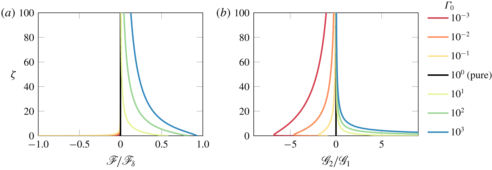
Figure 1. (a) Values of  $\mathscr{F}/\mathscr{F}_{\unicode[STIX]{x1D6FF}}$ versus $\unicode[STIX]{x1D701}$ and (b) $\mathscr{G}_{2}/\mathscr{G}_{1}$ versus $\unicode[STIX]{x1D701}$ for different values of $\unicode[STIX]{x1D6E4}_{0}$.
While (2.27) remains the apex contribution of the current analysis, an alternative solution approach to determine  $\unicode[STIX]{x1D701}_{avs}$ is to expand the bracketed term in (2.21) using the binomial theorem and integrate term by term to give
 $$\begin{eqnarray}\unicode[STIX]{x1D701}_{avs}=\frac{3\mathscr{B}_{\unicode[STIX]{x1D6FF}}}{4\unicode[STIX]{x1D705}Ri_{p}\unicode[STIX]{x1D6E4}_{0}^{1/2}},\quad \mathscr{B}_{\unicode[STIX]{x1D6FF}}:=\mathop{\sum }_{k=0}^{\infty }\frac{(\unicode[STIX]{x1D6E4}_{0}-1)^{k}}{k!(k(4\unicode[STIX]{x1D6FE}_{2}-5/2)+3/4)}\mathop{\prod }_{j=1}^{k}\left(\frac{1}{2}-j\right).\end{eqnarray}$$
 This solution, valid for  $0<\unicode[STIX]{x1D6E4}_{0}<2$, reduces to the constant- $\unicode[STIX]{x1D6FC}$ solution of Hunt & Kaye (Reference Hunt and Kaye2001) on setting $\unicode[STIX]{x1D6FE}_{2}=0$. Expressions (2.27) and (2.28a) scale identically on $Ri_{p}$ and $\unicode[STIX]{x1D6E4}_{0}$ and indeed are identical in the range $0<\unicode[STIX]{x1D6E4}_{0}<2$ (indicating that $3\mathscr{B}_{\unicode[STIX]{x1D6FF}}/4=4\mathscr{F}_{\unicode[STIX]{x1D6FF}}/3$).
Substituting for  $m$ from (2.26) into (2.19) gives the square of the volume flux
 $$\begin{eqnarray}q^{2}=\mathscr{G}_{1}+\mathscr{G}_{2}\quad \Rightarrow \quad q=\mathscr{G}_{1}^{1/2}\left(1+\frac{\mathscr{G}_{2}}{\mathscr{G}_{1}}\right)^{1/2},\end{eqnarray}$$
 where the functions  $\mathscr{G}_{1}(\unicode[STIX]{x1D6E4}_{0},\unicode[STIX]{x1D701})$ and $\mathscr{G}_{2}(\unicode[STIX]{x1D6E4}_{0},\unicode[STIX]{x1D701})$ are defined as
 $$\begin{eqnarray}\displaystyle & \displaystyle \mathscr{G}_{1}:=\unicode[STIX]{x1D6E4}_{0}^{2/3}C_{Q}^{2}Ri_{p}^{2/3}(\unicode[STIX]{x1D701}+\unicode[STIX]{x1D701}_{v})^{10/3}, & \displaystyle\end{eqnarray}$$
 $$\begin{eqnarray}\displaystyle & \displaystyle \mathscr{G}_{2}:=\frac{\unicode[STIX]{x1D6E4}_{0}-1}{\unicode[STIX]{x1D6E4}_{0}^{1-8\unicode[STIX]{x1D6FE}_{2}/3\unicode[STIX]{x1D705}}}(C_{Q}^{3}Ri_{p})^{16\unicode[STIX]{x1D6FE}_{2}/15\unicode[STIX]{x1D705}}(\unicode[STIX]{x1D701}+\unicode[STIX]{x1D701}_{v})^{16\unicode[STIX]{x1D6FE}_{2}/3\unicode[STIX]{x1D705}}. & \displaystyle\end{eqnarray}$$
 Since  $\mathscr{G}_{2}$ is associated with the non-pure adjustment behaviour, cf. (2.19b), the ratio $\mathscr{G}_{2}/\mathscr{G}_{1}\rightarrow 0$ in the limit as $\unicode[STIX]{x1D701}\rightarrow \infty$, provided $\unicode[STIX]{x1D6FE}_{2}/\unicode[STIX]{x1D705}\leqslant 5/8$, (n.b. which indeed is the case cf. table 1)
 $$\begin{eqnarray}\frac{\mathscr{G}_{2}}{\mathscr{G}_{1}}=\frac{\unicode[STIX]{x1D6E4}_{0}-1}{\unicode[STIX]{x1D6E4}_{0}^{(1-8\unicode[STIX]{x1D6FE}_{2}/\unicode[STIX]{x1D705})/3}}C_{Q}^{16(\unicode[STIX]{x1D6FE}_{2}/\unicode[STIX]{x1D705}-5/8)/5}Ri_{p}^{16(\unicode[STIX]{x1D6FE}_{2}/\unicode[STIX]{x1D705}-5/8)/15}(\unicode[STIX]{x1D701}+\unicode[STIX]{x1D701}_{v})^{16(\unicode[STIX]{x1D6FE}_{2}/\unicode[STIX]{x1D705}-5/8)/3}\end{eqnarray}$$
(see figure 1b).
Finally, substituting for  $m$ from (2.26a) into (2.19b), the variation of the local Richardson number $\unicode[STIX]{x1D6E4}(\unicode[STIX]{x1D701})$, indicating the imbalance from the equilibrium state, is
 $$\begin{eqnarray}\unicode[STIX]{x1D6E4}(\unicode[STIX]{x1D701})=1+(\unicode[STIX]{x1D6E4}_{0}-1)((\unicode[STIX]{x1D6E4}_{0}Ri_{p})^{2/3}C_{M})^{4(\unicode[STIX]{x1D6FE}_{2}/\unicode[STIX]{x1D705}-5/8)}(\unicode[STIX]{x1D701}+\unicode[STIX]{x1D701}_{v})^{16(\unicode[STIX]{x1D6FE}_{2}/\unicode[STIX]{x1D705}-5/8)/3}.\end{eqnarray}$$
3 Experiments
Particle image velocimetry measurements were acquired for negatively buoyant plumes formed by the injection of an aqueous-saline solution into a freshwater filled visualisation tank. Polyamide seeding particles with a nominal diameter of 50 μm and a density of 1.03 g cm-3 were used to seed the flow. PIV measurements were only conducted for plume release densities lower than 1.02 g cm-3 in order to minimise the optical distortion of particles owing to differences in refractive index between the saline release and the freshwater ambient. The Stokes velocity of the particles, estimated at 0.04 cm s-1, was considerably smaller than the centreline velocities recorded in the plume (1–7 cm s-1) such that the velocity lag experienced by the particles was expected to be minimal.
The videos were recorded at an acquisition rate of 30 f.p.s. with a shutter speed of 10 ms. A high aperture (F/1.4) was used to reduce the depth of field to a depth less than the thickness of the light sheet (the latter estimated at 10 mm). The PIV window was 180 × 360 mm2 (width by height) recorded with a resolution of 5 Megapixels (2048 × 2560). Particle scatter size roughly ranged between 3 and 5 pixels. A 15 pixel highpass filter was used to improve uneven lighting and a 5 pixel Wiener denoise filter was applied to reduce ghosting due to noise and unfocused particles. A two-pass interrogation scheme was adopted. Interrogation windows of area 128 × 128 and 64 × 64 pixels2 were used with a 50 % overlap for each window. Processing was conducted using a modified version of the open source software PIVlab from Thielicke & Stamhuis (Reference Thielicke and Stamhuis2014).
Plume nozzles with 44.5 mm and 89.0 mm diameters were used. The volume flux was estimated by integrating the time-averaged velocity field measured along the central plume axis and assuming rotational symmetry. The source volume flux was measured with an Apollo LowFlo flowmeter, with range 0.1–3.0 l min-1, and to an accuracy of ±1 % of the reading. The density of the saline solution and freshwater ambient was measured with an Anton Paar DMA 5000 density meter of accuracy ±0.0005 g cm-3.
The virtual origin correction  $\unicode[STIX]{x1D701}_{v\ast }$ was estimated from the volume flux measurements by defining it as
 $$\begin{eqnarray}\unicode[STIX]{x1D701}_{v\ast }:=\frac{q_{\ast }^{3/5}}{C_{Q}^{3/5}Ri_{0}^{1/5}}-\unicode[STIX]{x1D701}_{\ast },\end{eqnarray}$$
 where the asterisk subscript  $(\cdot )_{\ast }$ denotes a measured quantity. The maximum cumulative error $|\unicode[STIX]{x1D6FF}\unicode[STIX]{x1D701}_{v\ast }|$ on $\unicode[STIX]{x1D701}_{v\ast }$ was estimated to be ±11 %. The error on $C_{Q}(\unicode[STIX]{x1D6FE}_{1},\unicode[STIX]{x1D6FE}_{2})$ was estimated based on the historical values of $\unicode[STIX]{x1D6FE}_{1}$ and $\unicode[STIX]{x1D6FE}_{2}$ reported in table 1. Our estimates of the location for the virtual origin from (3.1) are shown in what follows by circular markers (●) with error bars overlain.
4 Results and discussion
The solutions for the  $\unicode[STIX]{x1D6FC}=\text{constant}$ and $\unicode[STIX]{x1D6FC}=\unicode[STIX]{x1D6FE}_{1}+\unicode[STIX]{x1D6FE}_{2}Ri$ formulations are expected to be indistinguishable in the far field, where locally the differences in behaviour between the actual plume and a pure plume are diminishingly small, irrespective of the source conditions (2.19b). This is confirmed in figure 2, which plots the streamwise variations of volume flux (figure 2a–c, from (2.29)) and momentum flux (figure 2d–f, from (2.26)), for example cases of forced ( $\unicode[STIX]{x1D6E4}_{0}=0.001$), pure ( $\unicode[STIX]{x1D6E4}_{0}=1$) and lazy ( $\unicode[STIX]{x1D6E4}_{0}=1000$) plumes. For the forced plume there is clearly a deficit in entrainment prevalent (lower volume flux) in the near-source region for the $\unicode[STIX]{x1D6FC}=\unicode[STIX]{x1D6FE}_{1}+\unicode[STIX]{x1D6FE}_{2}Ri$ formulation (blue line) when compared with the constant- $\unicode[STIX]{x1D6FC}$ predictions (red line); the trend in this region is reversed for lazy plumes. The variation of $\unicode[STIX]{x1D6E4}(\unicode[STIX]{x1D701})$ is plotted in figure 2(g–i). In both forced (figure 2g) and lazy (figure 2i) cases, the solutions indicate that the approach to pure behaviour is less rapid than predicted by constant- $\unicode[STIX]{x1D6FC}$ solutions.
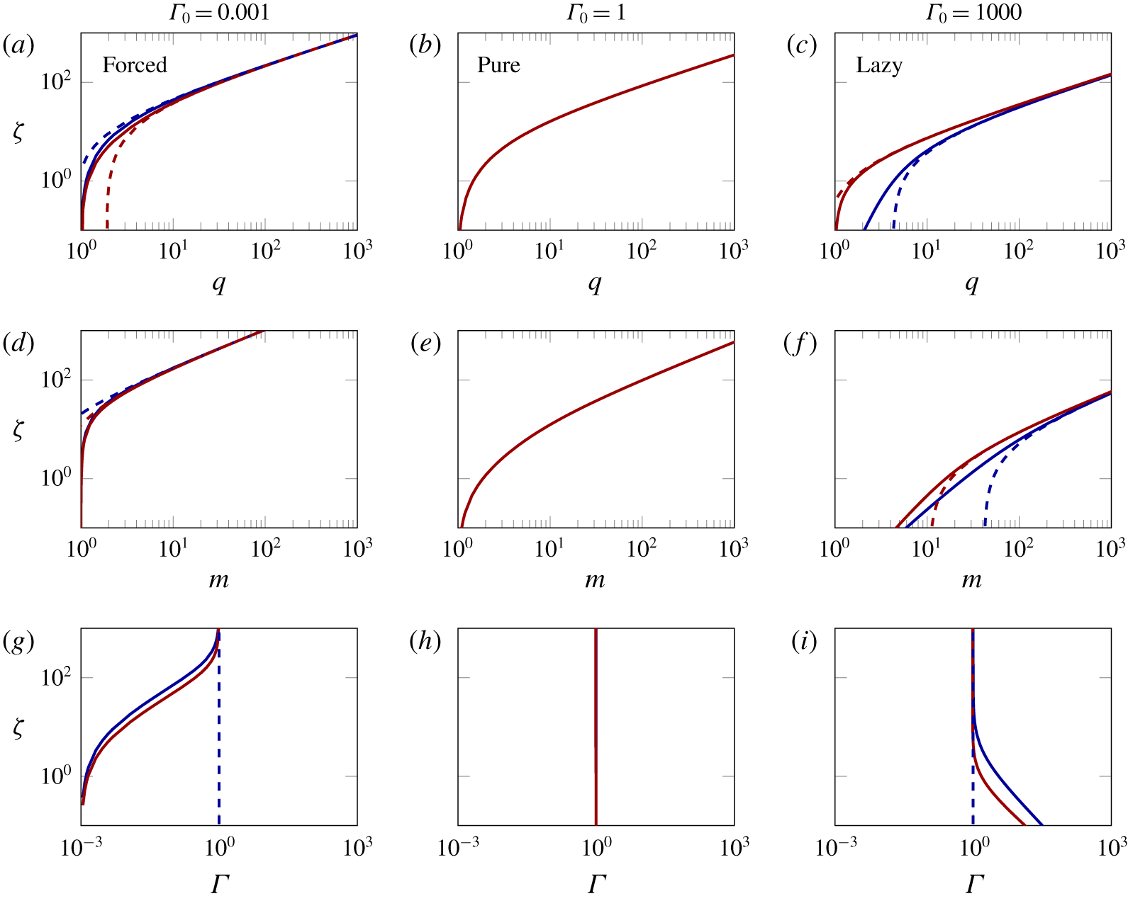
Figure 2. Values of  $q$ (a–c), $m$ (d–f) and $\unicode[STIX]{x1D6E4}(\unicode[STIX]{x1D701})$ (g–i) versus $\unicode[STIX]{x1D701}$ for $\unicode[STIX]{x1D6E4}_{0}=\{0.001,1,1000\}$, highlighting differences between the analytical solutions for $\unicode[STIX]{x1D6FC}=\text{constant}$ (solid red lines -) from Hunt & Kaye (Reference Hunt and Kaye2005), and for $\unicode[STIX]{x1D6FC}=\unicode[STIX]{x1D6FE}_{1}+\unicode[STIX]{x1D6FE}_{2}Ri$ (solid blue lines -) from (2.29), (2.26) and (2.33) (top-hat, $\unicode[STIX]{x1D705}=1$). Corresponding dashed lines show approximate solutions based on the virtual origin corrections given by Hunt & Kaye (Reference Hunt and Kaye2001, dashed red lines - -) and by (2.27, dashed blue lines - -). The $\unicode[STIX]{x1D6FC}=$ constant and $\unicode[STIX]{x1D6FC}=\unicode[STIX]{x1D6FE}_{1}+\unicode[STIX]{x1D6FE}_{2}Ri$ solutions overlie for the pure-plume case.
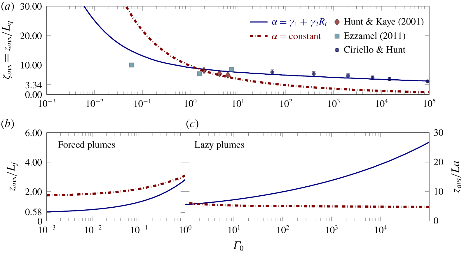
Figure 3. (a–c) Value of  $z_{avs}$ versus $\unicode[STIX]{x1D6E4}_{0}$ for $\unicode[STIX]{x1D705}=1$. Solution for $\unicode[STIX]{x1D6FC}=\text{constant}$ from Hunt & Kaye (Reference Hunt and Kaye2001, dot-dashed red line - ⋅-) and for $\unicode[STIX]{x1D6FC}=\unicode[STIX]{x1D6FE}_{1}+\unicode[STIX]{x1D6FE}_{2}Ri$ from ((2.27), blue line -). Markers plotted in (a) show experimental measurements from Hunt & Kaye (Reference Hunt and Kaye2001, ♦), Ezzamel (Reference Ezzamel2011, ▪) and our own PIV measurements of aqueous-saline plumes (§ 3, ●).
Our analytical solution (2.27) for the virtual origin correction  $\unicode[STIX]{x1D701}_{avs}=z_{avs}/L_{q}$, recalling $L_{q}=Q_{0}/M_{0}^{1/2}$, is plotted as a function of $\unicode[STIX]{x1D6E4}_{0}$ in figure 3(a) together with $\unicode[STIX]{x1D701}_{avs}$ inferred from integrating (2.11) numerically using a fourth-order Runge–Kutta method. Numerical and analytical solutions overlie so as to be graphically indistinguishable. Evidently, agreement between the prediction ((2.27), blue line -) and the data is good and improved over the constant- $\unicode[STIX]{x1D6FC}$ solution of Hunt & Kaye (Reference Hunt and Kaye2001, dot-dashed red line - ⋅-).
Physically, the magnitude of the virtual origin correction is indicative of the characteristic streamwise length over which the adjustment towards the pure-plume-like state occurs (Hunt & Kaye Reference Hunt and Kaye2001). Based on classically adopted scalings, the adjustment length is expected to scale on the jet length  $L_{j}:=M_{0}^{3/4}/B_{0}^{1/2}(\equiv L_{q}Ri_{0}^{-1/2})$ for forced plumes (Papanicolaou & List Reference Papanicolaou and List1988; Wang & Law Reference Wang and Law2002), and on the acceleration length $L_{a}:=Q_{0}^{3/5}/B_{0}^{2/5}(\equiv L_{q}Ri_{0}^{-1/5})$ for lazy plumes (Fischer et al. Reference Fischer, List, Koh, Imberger and Brooks1979; Hunt & Kaye Reference Hunt and Kaye2005). To assess this, figure 3(b) shows $z_{avs}/L_{j}$ and figure 3(c) shows $z_{avs}/L_{a}$.
For highly forced plumes ( $\unicode[STIX]{x1D6E4}_{0}\ll 1$, figure 3b) our solution (2.27) for the $\unicode[STIX]{x1D6FC}=\unicode[STIX]{x1D6FE}_{1}+\unicode[STIX]{x1D6FE}_{2}Ri$ formulation clearly shows $z_{avs}\sim O(L_{j})$, thereby confirming that the adjustment length does scale on the jet length. The distance between actual and virtual origins is less than that predicted by the Hunt & Kaye (Reference Hunt and Kaye2001) constant- $\unicode[STIX]{x1D6FC}$ model. Note that (2.27) gives
 $$\begin{eqnarray}\frac{z_{avs}}{L_{j}}=\frac{4}{3\unicode[STIX]{x1D705}Ri_{p}^{1/2}}\cdot \text{}_{2}F_{1}\left(\frac{1}{2};\frac{3}{8\unicode[STIX]{x1D6FE}_{2}/\unicode[STIX]{x1D705}-10};1+\frac{3}{8\unicode[STIX]{x1D6FE}_{2}/\unicode[STIX]{x1D705}-10};1\right)\approx 0.58\quad \text{for }\unicode[STIX]{x1D6E4}_{0}\ll 1.\end{eqnarray}$$
 For highly lazy plumes ( $\unicode[STIX]{x1D6E4}_{0}\gg 1$, figure 3c), our solution (2.27) for the $\unicode[STIX]{x1D6FC}=\unicode[STIX]{x1D6FE}_{1}+\unicode[STIX]{x1D6FE}_{2}Ri$ formulation shows that the adjustment length does not scale on the acceleration length scale (note the scale on the vertical axis). Instead, it follows from (2.27) that the virtual origin, and by extension also the adjustment length, scales on the plume radius at source
 $$\begin{eqnarray}\frac{z_{avs}}{L_{q}}=\frac{4}{3\unicode[STIX]{x1D705}Ri_{p}^{1/2}}\approx 3.34\quad \text{for }\unicode[STIX]{x1D6E4}_{0}\gg 1\end{eqnarray}$$
 (see figure 3a). By contrast, the solution for the constant- $\unicode[STIX]{x1D6FC}$ formulation, wherein $\unicode[STIX]{x1D701}_{avs}\sim \unicode[STIX]{x1D6E4}_{0}^{-1/5}$, appears to scale well on the acceleration length. This apparent change in adjustment length (from $L_{a}$ to $L_{q}$) has been observed in experimental measurements of highly lazy plumes (Kaye & Hunt Reference Kaye and Hunt2009), where the transition to a volume flux that varies as a 5/3rds power law occurs downstream of the neck of the plume and is independent of $\unicode[STIX]{x1D6E4}_{0}$. The solution (2.27) and $\unicode[STIX]{x1D701}_{avs}$ from Hunt & Kaye (Reference Hunt and Kaye2001) diverge as the acceleration length $L_{a}$ decreases with increasing $\unicode[STIX]{x1D6E4}_{0}$.
5 Conclusions
Our focus has been on developing analytical solutions that are applicable to turbulent plumes from area sources for which entrainment, varying locally in response to the fluxes of momentum, volume and buoyancy, is characterised by an entrainment function  $\unicode[STIX]{x1D6FC}$ that is linearly dependent on the local Richardson number. This form for the entrainment underpins our developments as it has been shown, both experimentally and numerically, to universally capture the behaviour of forced, pure and lazy plumes. We derive analytical solutions for the virtual origin, the fluxes of momentum and volume and the local Richardson number without placing restrictions on the source conditions. Our solutions thereby encompass the entire spectrum of forced, pure and lazy plume releases.
For forced and lazy releases, we show how the dynamical conditions in the plume approach the far-field equilibrium state of a pure plume and that this approach is less rapid than predicted under the assumption of invariant entrainment, i.e. for the widely adopted simplification  $\unicode[STIX]{x1D6FC}=\text{constant}$. Our solutions indicate that forced plumes adjust to become pure plume-like within a streamwise distance comparable to 60 % of a source jet length, while lazy plumes adjust within a distance comparable to three source radii. Finally, our analytical solution for the virtual origin agrees closely with data that span five orders of magnitude of source Richardson number, thereby giving us confidence in the application of this solution to general plumes from area sources.
Acknowledgements
G.R.H. gratefully acknowledges the EPSRC through grant no. EP/N010221/1, entitled Managing Air for Green Inner Cities (MAGIC).
Declaration of interests
The authors report no conflict of interest.
Appendix A. The entrainment function of Carazzo et al. (Reference Carazzo, Kaminski and Tait2006)
Carazzo et al. (Reference Carazzo, Kaminski and Tait2006) propose an entrainment function in the form
 $$\begin{eqnarray}\unicode[STIX]{x1D6FC}=\unicode[STIX]{x1D6FE}_{1}+\unicode[STIX]{x1D6FE}_{2}Ri+\frac{\text{d}\unicode[STIX]{x1D6FE}_{3}}{\text{d}\unicode[STIX]{x1D701}},\end{eqnarray}$$
 where  $\unicode[STIX]{x1D6FE}_{3}$ is a higher-order integral property that depends on the velocity, buoyancy and turbulent stress profiles. As noted by van Reeuwijk et al. (Reference van Reeuwijk, Salizzoni, Hunt and Craske2016), the third term, $\text{d}\unicode[STIX]{x1D6FE}_{3}/\text{d}\unicode[STIX]{x1D701}$, compensates for the adjustment in velocity and buoyancy profiles and can, as a result, be neglected in a time-averaged analysis. Our solutions are consistent with the model (A 1) in that we specify that the profiles are assumed to be either top-hat or Gaussian.
Appendix B. Two-dimensional plumes
Defining a pure-plume Richardson number as  $Ri_{0L}=B_{0L}Q_{0L}^{3}/M_{0L}^{3}$ and scaled source Richardson number as $\unicode[STIX]{x1D6E4}_{0L}=Ri_{0L}/2\unicode[STIX]{x1D6FC}_{p}\unicode[STIX]{x1D705}$, the conservation equations for a two-dimensional plume of dimensionless volume and momentum fluxes per unit length of the source, $q_{L}$ and $m_{L}$, can be deduced to give
 $$\begin{eqnarray}\frac{\text{d}q_{L}}{\text{d}\unicode[STIX]{x1D701}_{L}}=\unicode[STIX]{x1D6FE}_{1L}\frac{m_{L}}{q_{L}}+\unicode[STIX]{x1D6FE}_{2L}Ri_{pL}\frac{q_{L}^{2}}{m_{L}^{2}}\quad \text{and}\quad \frac{\text{d}m_{L}}{\text{d}\unicode[STIX]{x1D701}_{L}}=\unicode[STIX]{x1D705}Ri_{pL}\unicode[STIX]{x1D6E4}_{0L}\frac{q_{L}}{m_{L}},\end{eqnarray}$$
 where  $\unicode[STIX]{x1D701}_{L}=zM_{0L}/Q_{0L}^{2}$. Combining (B 1a,b) one may obtain the solutions
 $$\begin{eqnarray}q_{L}^{3}=\frac{m_{L}^{3}}{\unicode[STIX]{x1D6E4}_{0L}}+\frac{\unicode[STIX]{x1D6E4}_{0L}-1}{\unicode[STIX]{x1D6E4}_{0L}}m_{L}^{6\unicode[STIX]{x1D6FE}_{2L}/\unicode[STIX]{x1D705}}\quad \text{and}\quad \unicode[STIX]{x1D6E4}_{L}=1+(\unicode[STIX]{x1D6E4}_{0L}-1)m_{L}^{6\unicode[STIX]{x1D6FE}_{2L}/\unicode[STIX]{x1D705}-3}.\end{eqnarray}$$
 A virtual origin correction for a two-dimensional plume with a linear  $Ri$ entrainment function is reported in van den Bremer & Hunt (Reference van den Bremer and Hunt2014), their appendix A. Following the approach developed herein (§ 2), the correction can be expressed in terms of hypergeometric functions as
 $$\begin{eqnarray}\unicode[STIX]{x1D701}_{avs,L}=\frac{\mathscr{F}_{\unicode[STIX]{x1D6FF},L}}{\unicode[STIX]{x1D705}Ri_{pL}\unicode[STIX]{x1D6E4}_{0L}^{2/3}},\end{eqnarray}$$
where
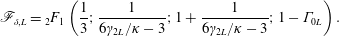 $$\begin{eqnarray}\mathscr{F}_{\unicode[STIX]{x1D6FF},L}=\text{}_{2}F_{1}\left(\frac{1}{3};\frac{1}{6\unicode[STIX]{x1D6FE}_{2L}/\unicode[STIX]{x1D705}-3};1+\frac{1}{6\unicode[STIX]{x1D6FE}_{2L}/\unicode[STIX]{x1D705}-3};1-\unicode[STIX]{x1D6E4}_{0L}\right).\end{eqnarray}$$
It should be noted that there is, as yet, no experimental evidence that supports the notion of a linear entrainment function for two-dimensional lazy plumes.


 Open access