


Introduction
Monte Carlo simulations are widely used in applications related to both electron beam imaging and microanalysis [Reference Walker1]. They provide information such as the interaction volume of incident electrons and X-ray distributions [Reference Morozov2], and they are useful in cathodoluminescence emission measurements [Reference Toth and Phillips3] and mass thickness estimations [Reference Moro4,Reference Pazzaglia5]. They also compute backscattered and secondary electron yields, which are important for image simulations used to estimate signal variations [Reference Mir6,Reference Yio7] and secondary election emissions of electrode materials [Reference Chang8]. Finally, a crucial use of Monte Carlo simulations is to perform accurate elemental quantification from energy-dispersive spectroscopy (EDS) data. Matrix correction factors can be computed using Monte Carlo simulations and then used to calculate accurate compositional information from X-ray intensities [Reference Donovan9–Reference Brodusch and Gauvin11]. This allows quantification to be done without the need for standards or pre-measured experimental databases [Reference Horny10].
The most widely used programs available are PENEPMA, CASINO, and DTSA-II [Reference Llovet and Salvat12–Reference Ritchie14]. While these programs have been well adapted for common uses in electron microscopy and microanalysis, there exist some limitations to their usability. The most notable of these are the computation time and restrictions on sample and microscope geometries. For example, simulations of electron numbers on the order of 105 at a single point may take approximately a minute on a desktop computer [Reference Ritchie15]. These long computing times can make simulations of backscattered electron (BSE) images or EDS maps unfeasible in a reasonable amount of time. The limitations in terms of geometry impact the usability of these programs on complex materials. Important obstacles arising from non-flat sample geometries can strongly impact accurate elemental quantification [Reference Newbury and Ritchie16,Reference Newbury17]. To simulate such materials, freedom in terms of sample and microscope geometry and placement must be possible.
Here, we present the incorporation of the existing Monte Carlo software MC X-ray [Reference Gauvin and Michaud18] into the image processing software Dragonfly developed by Object Research Systems (ORS) Inc. [19]. The class system of Dragonfly allows substantial freedom in terms of sample geometry and placement. Furthermore, additions have been made to turn MC X-ray into a full microscope simulation tool capable of reproducing some elements of an electron microscope. Multiprocessing has also been implemented to decrease computing times substantially, allowing more complex problems to be easily evaluated. The manuscript is structured as follows. First, the details and usability of the program are described with reference to previous Monte Carlo software. Then applications of the library to BSE image simulations and elemental quantification are presented. Finally, some concluding remarks are made about the method.
Materials and Methods
MC X-ray is a Monte Carlo-based simulation package [Reference Gauvin and Michaud18] that was devised as an extension of CASINO [Reference Hovington13,Reference Drouin20] and Win X-ray [Reference Gauvin21], specific for X-ray microanalysis. Scattering events are modeled based on a stochastic process where electrons are simulated using a forward scattering random walk. An electron is initiated, and uniform random numbers are generated and used in cross-sectional models to determine the particle's path through the sample material. The physical models, methodology, and calculations used are described in other work [Reference Gauvin21]. The previously stand-alone MC X-ray program was incorporated into the image processing software Dragonfly as a feature plug-in. The base code was written in C++, and the interface used to gather the input and call the simulation functions was written in Python 3.
Sample generation is done using the Multi-region of interest (ROI) class inside Dragonfly. A phantom material is created as a MultiROI where each subgeometry is its own ROI. The structures are voxel-based where the dimensions of the voxels are chosen by the user. Once a phantom has been defined, labels may be assigned to each ROI. Each label contains a property where, for the purpose of libMCXray, these properties represent the constituent elements of each region. The labels are vectors whose lengths are the number of regions and whose values are the composition of the elements in the indexed region. Thus, a material may be generated with a multitude of elements in a variety of regions with varying compositions. MultiROIs can be created by the user or generated from other image data such as stacks of images, which can be compiled into a 3D structure.
The simulation environment comprises an electron beam, a sample material, and a series of detectors. The electron beam is above the sample material normal to its surface. The user input parameters of the beam are the incident electron energy, incident current, and working distance. The rasterizing across the sample surface is done by displacing the beam across the sample surface at steps specified by the user input resolution. Once the sample material is constructed, it is placed so that the beam and the sample are along the same axis. Their vertical distance is specified by the desired working distance.
Detectors may then be added to the simulator. The BSE detector may be defined as a disc or circular annulus below the electron gun. The input in this case is the inner and outer radius of the annulus or the radius of the disc. BSEs are defined as those which have exited the sample and intersected the detector. The EDS detector is defined by the properties specified in Table 1 and are similar to the stand-alone version of MC X-ray. Multiple detectors can be added to the simulator, each with their own properties. Last, bright-field and dark-field detectors can be added below the sample. Each is defined by their distance from the exit surface of the sample and their inner and outer solid angles. Again, intensities of either signal are constructed from the number of electrons intersecting the respective detectors upon exit from the sample.
Table 1: EDS detector parameters modifiable by user in libMCXray.

The program output is separated into two parts: electron and X-ray data. From the rasterizing, the BSE image and any possible transmitted signal images are output as 2D arrays of floating-point real numbers. The EDS maps are output as 3D arrays where the first two dimensions are the point coordinates and the third dimension is the energy spectrum. Finally, if point analyses are chosen, the X-ray depth distribution curves, ϕ(ρz), of specified transitions may be output.
Results and Discussion
BSE image simulation
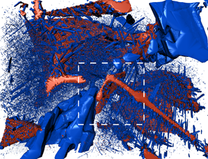
A MultiROI of a three-phase alloy compiled from a focused ion beam image dataset was used to simulate backscattered images. A 3D perspective of the MultiROI is depicted in Figure 1. Elemental compositions were assigned to the phases prior to performing the Monte Carlo simulation. A Ni-Fe-Cr system was investigated where each element was associated to a pure single phase. The phases to which each element is associated are presented in Table 2. The incident probe position was rasterized across the top surface of the sample shown in Figure 1. The sample plane at the incident direction is displayed in Figure 2.

Figure 1: 3D representation of sample geometry used in simulation experiment. Phase 1 is the matrix, phase 2 is in red, and phase 3 is in blue. The matrix phase is transparent.

Figure 2: View of simulated material from beam incident direction. The area across which the beam was rasterized is indicated by a dashed rectangle.
Table 2: Compositions of the simulated system assigned to the MultiROI of Figure 1.

Simulations were performed at 15 keV using 5,000 electrons. Because the simulations of each probe position are independent, the method is easily parallelized, allowing for an acceleration of 80 to 100 times the computing time of the original program. The simulated BSE image corresponding to a subsection of the incident plane of Figure 2 is presented in Figure 3.

Figure 3: Simulated BSE image of three-component Ni-Fe-Cr system at 15 keV using libMCXray.
The image consists of 512 × 512 pixels situated about the center of the plane. This area is indicated in Figure 2 by a dashed rectangle. Here, the three pure element phases are clearly distinguished with the fine structures from the underlying geometry clearly visible. The differences in signal level clearly reflect the differences in atomic number between each phase. The matrix is composed of pure Ni, the heaviest of the three elements, whose signal level is the highest. In comparison, the Cr phase, contained in the majority of the needle-like structures, is seen as the phase containing the lowest level of signal, consisting of points attached to the Fe phase and the large rectangular structure in the bottom right corner of the image.
Another system was simulated consisting of the expected phases of an Al-Si alloy to show the versatility of the method in simulating alloys closer to reality. Figure 4 shows a simulated BSE image of the same geometric structure, however here the phases consisted of pure Al as the matrix, phase 1, Al2Cu as phase 2, and Mg2Si as phase 3. Simulations were performed under the same conditions as the Ni-Fe-Cr system.

Figure 4: Simulated BSE image of Al-Si alloy containing three phases: pure Al, Al2Cu, and Mg2Si.
Because Cu has a much higher atomic number than the other constituent elements, and hence a higher probability of scattering, the signal level of the Al2Cu phase is the highest in the image. In comparison, the Mg2Si phase contains the lowest signal level due to its lower probability of scattering. This demonstrates that even multi-component phases may properly and easily be simulated using libMCXray, and the attributes of the Dragonfly software aid in proper image analysis.
EDS spectrum analysis and mapping
EDS maps were simulated for the above system using the same MultiROI and positions. Here, 2048 channels were used across the energy scale. Figure 5 shows the entire 3D dataset acquired using libMCXray, two spatial dimensions and the third in energy. The EDS simulation was performed on the Amazon AWS high-performance computing (HPC) network and took 1 hour on 500 computers each containing 8 cores. On an extremely performant workstation, such a simulation would take approximately 200 hours. Computing times are rendered much more reasonable by the use of cluster computing.

Figure 5: Three-dimensional depiction of the EDS dataset simulated using libMCXray. The image represents spatial dimensions of 512 × 512 pixels and 2048 energy bins.
Slices of the dataset were taken at the corresponding Kα transition energies for each element. These slices are depicted as 2D maps in Figure 6.

Figure 6: Simulated EDS maps for (a) Ni Kα, (b) Fe Kα, and (c) Cr Kα transitions. These correspond to 7.477, 6.403, and 5.414 keV respectively.
The simulated EDS maps correspond exactly to the BSE image and simulated geometry. Areas of white imply areas of high intensity, while black describes areas of low to no intensity. The simulated spectrum at a point is depicted in Figure 7 along with the BSE image showing the point at which the spectrum was taken.

Figure 7: (a) BSE image showing the point at which an energy spectrum was taken and (b) corresponding energy spectrum showing peaks from Ni, Fe, and Cr. The labels are placed above the Kα peaks.
At this point, contributions from all three phases are present. Although these results are all simulated, the accuracy of MC X-ray simulations for K-shell ionizations has been demonstrated in previous work [Reference Wuhrer and Moran22–Reference Teng25].
Conclusions
The Monte Carlo simulation program MC X-ray was incorporated into the Dragonfly software package by ORS to simulate BSE imaging and EDS analysis inside an all-encompassing image processing software. Using parallelization and good software practice, the calculation speed was improved by ~80–100 times the original code. Furthermore, using the Dragonfly interface, complex geometries may be created or even imported from datasets such as those generated in focused ion-beam experiments. Future work will see the addition of secondary electron detection and the incorporation of higher-order ionization effects such as secondary fluorescence yields.


