

After the failed convertibility attempt of 1947, the 1949 devaluation demonstrated that sterling still played an important role when it came to Europe. Governments across the continent, aware that their currencies were overvalued against the dollar, waited for sterling to devalue before they followed. More than nineteen countries followed sterling. The devaluations reshuffled the whole currency equilibrium not only in Europe but across the world. The devaluation also laid the ground for negotiations that would lead to the European Payments Union (EPU).
What is not clear is whether the devaluation was triggered by external international pressures or if the decision was based on domestic policy. The timing of the devaluation suggests that British policymakers took the decision to devalue only once reserves were exhausted. Using new archival materials, I demonstrate that the key issue was a worsening of the balance of payments. From May to August 1949, imports from the United States saw an up to six-fold increase. These spikes were mainly due to two factors: worsening economic conditions in the United States, and speculation through leads and lags.Footnote 1 I establish a precise timeline for the run on the pound by using daily data, which was unavailable in previous research.
Claudio Borio and Gianni Toniolo argue that the 1949 devaluation and the realignment of currencies were planned in a ‘coordinated fashion, reflecting the new postwar cooperative mood, and moved exchange rates closer to the purchasing power parity of European currencies’.Footnote 2 Despite more coordination among central banks, the timing of the devaluation was very much an internal decision made by the British government. While Borio and Toniolo are right to emphasise that there was more cooperation during that period, Britain’s decision to devalue was made without regard to the international situation.Footnote 3 US policymakers did use the threat of withdrawal of funding through the Marshall Plan or other means as a way to force Britain to comply. But at the end of the war, Britain still believed it played a major role in the world and was not keen to compromise.
This chapter also explores the impact of the 1949 sterling devaluation on US policies and monetary gold reserves. The 1949 devaluation marked a shift in US gold accumulation. Monetary gold reserves had been increasing since the war but the 1949 devaluation would reverse this trend. And during this period, there was an increase in demand for gold relative to the dollar, a phenomenon referred to as the dollar gap.Footnote 4
The Politics of the Devaluation
The British government and Bank of England were for the most part against devaluation. On the other side of the Atlantic, the IMF and US government were in favour of it. In late 1948, the British Board of Trade suggested devaluing sterling. But Harold Wilson, who presided over the Board at the time, was opposed to the idea.Footnote 5
In March 1949, a recession in the United States began to have an impact on Britain. At this point, Sir Robert Hall, director of the Economic Section of the Cabinet Office, ‘initiated a campaign to change minds in the Treasury and Foreign Office in favour of devaluation’.Footnote 6 The Chancellor of the Exchequer, Sir Stafford Cripps, was the principal opponent.Footnote 7 In July, however, Cripps went to Switzerland for medical treatment as he was suffering from abdominal cancer. His absence resulted in mounting pressure on the Cabinet to devalue.Footnote 8 Hugh Gaitskell, Minister of Fuel and Power and a figure of increasing importance in the Cabinet, believed that ‘devaluation might buy the government a brief “lull” in economic conditions’.Footnote 9 This would allow Labour to call a general election ‘before it had to put further controls on consumption and imports’, a decision that would prove electorally unpopular.Footnote 10 Morgan Phillips, general secretary of the Labour Party, wanted to call an election well after the devaluation. He opposed Gaitskell’s strategy. Philips did not prevail and the election was held in February 1950, just a few months after the devaluation.
According to Cairncross and Eichengreen, most of the officials at the Bank of England were against devaluation.Footnote 11 Still, the Bank was preparing for it and, as early as February 1948, was working on a devaluation communication plan. The goal was to assess how much notice to give to other sterling area countries, the United States and international institutions.Footnote 12 The main questions were who to communicate with and when. The Bank of England revised this communication plan frequently and several drafts have been kept in its archive. The first drafts mention partner countries and institutions to contact, but next to ‘U.S.A.’ there are two question marks. The Bank was not sure when to involve the United States in the process. In later drafts, the authors of the memo listed the United States as a country to be consulted between two and six days before the devaluation. This was still relatively short notice for an important partner such as the United States. The risk was that the information would leak. A leak would create a run on sterling before the official devaluation.
As the US government was pushing the United Kingdom to devalue, it expected more transparency. During a meeting in June, William McChesney Martin, who at the time worked for the US Treasury Department, stressed ‘the importance of consultation prior to action’ and that the IMF would have a role to play in a devaluation.Footnote 13 Willard Thorp, of the US State Department, also stressed ‘the need for close cooperation’, noting that ‘we had passed out of the honeymoon phase of the ERP program’.Footnote 14 The US government was informed in June 1949 of ‘the possibility that the UK may be confronted this summer with a major financial crisis not unlike that which developed in 1947’.Footnote 15 In early September, the US position became clear. The United Kingdom had to inform US officials not of ‘the precise rate to which they propose to devalue or the precise day on which they would expect to make their approach to the International Monetary Fund’, but they should ‘have a rough idea’.Footnote 16 The constant demands for information-sharing show that in this period, British policymakers did not see the United States as a partner in its domestic decision-making. US policymakers in turn thought that devaluation was a decision the United Kingdom should make ‘in its own interest, if it has a realistic view of its own situation’.Footnote 17
The IMF was in favour of devaluation and made this public.Footnote 18 Harold James argues that the IMF thought a devaluation was necessary to ‘clear the way for general European adjustment’.Footnote 19 An IMF report of May 1949 notes that ‘U.K. export prospects in the U.S. and Canada would be improved by a parallel devaluation of currencies other than the U.S. and Canadian dollars’.Footnote 20 Schenk describes how the IMF consulted European nations in May and June 1949 and concluded that ‘any general change of rates would have to be led by a devaluation of sterling’.Footnote 21 The fact that the IMF was consulted, Schenk argues, is proof that the devaluation was implemented with the IMF’s blessing.
The 1949 devaluation took place with pressure from the United States to stabilise the European situation. The United States was emerging as a world leader and in response began imposing its views on Europe. Still, the ultimate decision to devalue, and the process that led to it, remained very much within Britain’s domain.
Causes of the Devaluation
Explanations for the 1949 sterling devaluation have emphasised the role of a structural trade deficit with the dollar area. Another cause was a minor recession in the United States in the second quarter of 1949, followed by speculation against the pound. And finally, political pressure from the United States played a role.
The literature is unanimous in the belief that the devaluation was predictable. Cairncross and Eichengreen highlight the ‘growing conviction in financial circles that the current exchange rate would eventually have to be devalued’. Howson writes that it ‘was always likely that Britain would have to devalue the pound’. Schenk argues that a ‘gradual build-up of evidence and opinion’ led to devaluation. Capie and Wood refer to ‘outside opinion’ waiting for devaluation.Footnote 22
Contemporary observers were aware that devaluation was imminent and the Economist in April reads:
There is a steadily mounting volume of discussion throughout the world of what is somewhat euphemistically referred to as an adjustment of currencies but what it would be more honest to call the devaluation of all the world’s soft currencies. All over Europe it is a general topic of speculation in one, if not the other, meaning of the word.Footnote 23
Even Cripps later admitted that it was expected: ‘Our action had been discussed, debated, and indeed almost expected, throughout the world.’Footnote 24
The decline in reserves leading to devaluation was largely due to three factors: a recession in the United States; stockpiling; and speculation through leads and lags, which worsened the dollar balance of payments.
Leads and lags occur when importers and exporters speculate by adjusting the terms of payments.Footnote 25 For instance, a British importer could stockpile goods bought in dollars, hoping for a devaluation. Later, they would make a profit when the price of the goods from the dollar area increased as a result of the devaluation. British exporters could ease the terms of payment of their US counterpart. They could move the payment terms from, say, thirty to ninety days, to be paid after the devaluation.Footnote 26 It would be a bet that the devaluation would occur between thirty to ninety days after delivery of the goods. In his essay ‘Leads and Lags: The Main Cause of Devaluation’, Paul Einzig argues that the ‘main reason why the Government felt impelled to dishonour its pledges and devalue sterling was because of persistent selling pressure caused by leads and lags’.
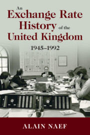
Contemporaries were aware of leads and lags. On 9 July 1949, The Financial Times observed that ‘in recent months the growing fear of sterling devaluation has sped up sales to Britain and has slowed purchases and the payment for them’.Footnote 27 The British Ambassador to the United States mentioned the issue. He explained: ‘withholding of payments by US importers, slower repatriation of dollar receipts by UK and Empire exporters and some postponement of purchasing commitments by US and other countries, all of these traceable to widespread talk about possible sterling devaluation’.Footnote 28 The Bank for International Settlements (BIS) reported that ‘foreign importers of sterling goods delayed their orders and payments, while sterling-area importers tried to speed up purchases and payments as much as they could’.Footnote 29 Leads and lags were putting a strain on British reserves, as Figure 2.1 illustrates.

Figure 2.1. EEA dollar and overall reserves
Note: Overall reserves are on the left scale, EEA dollar reserves (in $ million) are on the right scale. The overall reserves are the sum of the gold and dollar reserves (other currencies were negligible).
In 1949, Exchange Equalisation Account (EEA) dollar and gold reserves dropped by more than 40 per cent. They moved from £318.2 million in January to £190.2 million in early September, before the devaluation.Footnote 30 The loss represents $517.1 million at the official $4.03/£ parity. The most striking result can be seen in the EEA dollar account, which was almost emptied. The account held only $3.2 million at its lowest point on 7 September 1949, from just under $300 million in April (Figure 2.1). At the beginning of the run on sterling, the losses can be seen only in the dollar account.
The gold reserves fell later than the dollar reserves. Between June and September, the EEA sold over £86 million of gold to buy dollars. Until June, the EEA bought gold from South Africa against sterling, which explains the delay in the drop of overall reserves. The dollar account suffered dramatic losses starting in March 1949.
The Balance of Payments Problem
At the heart of the 1949 crisis lay balance of payments problems. This was not the overall balance of payments, which had been improving since 1947, but the trade deficit with the dollar area.Footnote 31 In previous research, data on the trade deficit have been collected by the quarter and usually from statistical yearbooks.Footnote 32 Here I use the confidential monthly reports on external finance. These reports circulated in numbered copies between the Bank of England, the Treasury and the Cabinet. These are the data policymakers used to decide on the future of sterling. I use these data to show evidence of the channels through which leads and lags went. Previous literature mentions leads and lags but does not provide data to substantiate their existence.Footnote 33
Figure 2.2 presents the dollar deficit. The worst trade deficits for the sterling area since 1947 (the year of the convertibility crisis) occurred during May to August 1949. Deficits for these four months are 57–81 per cent higher than the average of the preceding twelve months. The losses in these months provide an explanatory factor for the drop in EEA reserves. Marshall Plan aid was insufficient to mitigate the losses suffered. Despite these losses, officials were wary of publicly increasing drawings from the Marshall Plan as this would cause the market to react negatively. During this same period, the EEA’s combined gold and dollar reserves fell below £300 million for the first time. The 1949 crisis draws its roots from losses during these few months.
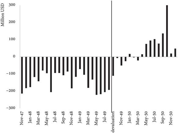
Figure 2.2. Variation of the overall sterling area balance of payments in millions as the sum of all the sterling area deficits with the non-sterling area
In the monthly reports, British imports are divided into six categories: food and drink, tobacco, raw materials, oil, machinery and other manufactures, and others.Footnote 34 The reports organise exports into three categories: exports and re-exports, diamonds and others.
Do these import and export figures for May to August 1949 stand out when compared with the averages for these months in other years? This would indicate speculation against the pound. It is unlikely that anything else would suddenly increase the country’s need for, say, food and drink, assuming that the population size remains constant.
Seasonality concerns require a comparison with similar months. To mitigate this, I compare the trade figures for May–August 1949 with the average for May–August 1948 and 1950 together. For example, in summer there would probably be more imported beverages consumed. But this would not change much from one summer to the next. Table 2.1 presents the results. To check the robustness of my findings, I also compared May–August 1949 to the twelve months before the devaluation. The results are broadly similar, but I do not show them here.
Table 2.1. Percentage increase/decrease of British exports, imports and trade deficit with the United States
| UK imports | May-49 | Jun-49 | Jul-49 | Aug-49 |
|---|---|---|---|---|
| Food and drink | 700% | 918% | 736% | 155% |
| Raw materials | 180% | 180% | 57% | 57% |
| Oil | 13% | –29% | –8% | 27% |
| Machinery and other manufactures | 51% | 87% | 44% | 8% |
| Total UK imports | 77% | 86% | 45% | 53% |
| UK exports and re-exports | –35% | –39% | –15% | –31% |
In absolute terms, the UK trade deficit with the United States for May–August was $307 million, 1.36 times the EEA dollar reserve at the beginning of 1949. Without Marshall Aid, the government would have been forced to devalue earlier. The figures in Table 2.1 are only imports and exports with the dollar area. The dollar area is where the United Kingdom was spending dollars needed by the Bank of England to defend the pound. In June 1949, food and drink imports were more than ten times higher than in the previous and following years. This stands out, and shows that it was most likely due to speculation. Equally, exports for these four months were down by approximately a third. Here also speculation is the likely culprit, and not a change in economic activity.
Why did imports rise tenfold and exports drop by a third for this period? Leads and lags offer the most convincing explanation. As seen earlier, contemporary economists and analysts reported the practice. To find evidence in the data, a closer look is needed. When analysing import and export data just before and after the devaluation there seems to be evidence of the practice. The rise in imports and fall in exports presented in Table 2.1 is the first explanation. But leads and lags also played a role after September 1949. Following a devaluation, at least in the short term, economists at the time agreed that exports were expected to rise and imports fall, as demand for domestic products increased, substituting for more expensive products.Footnote 35 Therefore, the expected short-term effect would be to see imports decrease and exports rise.
When looking at the data on exports to the United States in Figures 2.3 and 2.4, the effect is different. First, before the devaluation exports dropped drastically. This is due to exporters waiting for a devaluation before requiring payment from their counter-parties. After the devaluation there was a sharp increase in exports, but this lasted only two months. The peak in exports shows exporters being paid after the devaluation. On the import side, a similar occurrence can be seen. Importers were heavily stockpiling before the devaluation. Then, they used their stocks for the months following the devaluation when imports paid for in sterling were more expensive. These figures, presented here for the first time, offer further evidence of leads and lags.
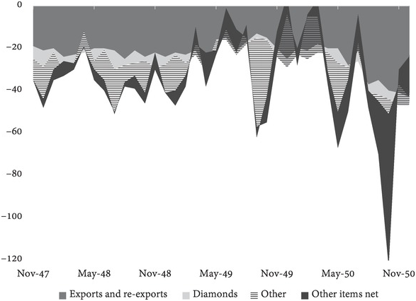
Figure 2.3. UK exports with the dollar area

A few years after these events, the Radcliffe Report summarised the devaluation: ‘Devaluation may take place as the only way out of an exchange crisis rather than a deliberate decision of policy.’Footnote 36 This is what happened in 1949, as the loss of reserves shows. The report continues, ‘but in that event, it is likely to be due to earlier policy decisions or failure to take them in time’. In 1949, the government failed to devalue before devaluation debates became public knowledge. This cost the United Kingdom valuable reserves. The devaluation occurred when Marshall Aid could no longer finance the reduction in reserves. The government decided to devalue not because of political pressure from abroad, but because of a run on sterling. Despite capital controls, the run operated through leads and lags. The deviation of imports and exports figures from previous trends makes this clear, and additional evidence comes from the drop in exports and increase in imports just before the devaluation, which was then reversed. What were the international repercussions of the devaluation?
International Repercussions
The IMF and the United States wanted Britain to lead the rest of the world in adjusting the value of the dollar.Footnote 37 Nineteen countries followed sterling in the currency adjustment. The BIS noted that since the gold standard was first established, ‘there have been only two years in which adjustments of foreign exchange rates have been so sweeping that the expression “wave of devaluations” has been justified’.Footnote 38 Table 2.2 summarises this ‘wave’ using an article in the Economist published a few days after the devaluation. It presents a list of all countries that followed the United Kingdom into devaluation. Sterling’s importance meant that most countries did so. With the approval of the IMF and the United States, even countries outside the sterling area devalued. This was the case for France, the Netherlands, Portugal and Sweden, among others. Most countries devalued by 30.5 per cent against the dollar. The last group in the table, however, did not change parity with the dollar and consequently also revalued their currency by 30.5 per cent against sterling.
Table 2.2. Devaluation against the dollar by country
| Country | Devaluation |
|---|---|
| Australia, Burma, Ceylon, Denmark, Egypt, Finland, Greece, India, Iraq, Ireland, Israel, Netherlands, New Zealand, South Africa, Sweden, UK | 30.5% |
| France | 22.2% |
| Portugal | 13.3% |
| Belgium | 12.3% |
| Canada | 9.1% |
| Czechoslovakia, Pakistan, Persia, Poland, Switzerland | No devaluation against the dollar |
Note: The table is missing Germany which also devalued the Deutschmark by 20.7%.
Beyond political coordination, did the 1949 devaluation reduce global economic imbalances? Was this sterling-led move beneficial for the stability of the international monetary system? Parallel market data show that the devaluation reduced global imbalances. Carmen Reinhart and Kenneth Rogoff provide a data-set of parallel markets for ninety-three countries.Footnote 39 The premium is calculated as a percentage of the official rate. The data comes from either free markets or black markets. Reinhart and Rogoff compute the market premia as follows: premium = (parallel – official)/official. A premium of 100 means the parallel market rate is twice the official rate. A premium of 0 means that parallel rates are the same as the official rate, which is the case for most exchange rates in a mobile capital economy. Figure 2.5 presents the average of the premium index for ninety-two countries from the Reinhart and Rogoff sample.Footnote 40
Figure 2.5. Average parallel (black or free) market premium, average of ninety-two countries
Figure 2.5 shows the rapid decline in parallel market premia, based on Reinhart and Rogoff. The index falls from almost 100 before the devaluation to around 50 six months later. For example, sterling traded around $2.4 on free markets in Switzerland and $4.03 in the official market. As a result of the sterling devaluation, the Reinhart and Rogoff index for the pound declined from a 42.4 per cent discount to a 9.8 per cent discount. After the devaluation, the average black and free market premia for the ninety-two countries from the sample dropped drastically and did not return to pre-devaluation levels until the 1960s. The devaluation played a positive role in the reduction of free market premia. This also meant less tension on global capital market and less illegal arbitrage.
The devaluation dealt with global imbalances as it reduced black market premia worldwide. It prepared the ground for the EPU. But what was the effect of the devaluation on the world’s leading currency, the dollar? And what effect did it have on the Federal Reserve? The devaluation of nineteen currencies against the dollar is akin to a revaluation of the dollar. The effects were also felt in the short run and the mechanism was as follows: The United Kingdom experienced large capital outflows during the run-up to the devaluation. Investors, importers and exporters all tried to move their assets out of sterling into the most liquid and safe currency, the dollar. After the devaluation, they repatriated their capital to the United Kingdom or the sterling area. This large inflow of dollars ended up in the hands of the Bank of England, which did not want such large dollar holdings and preferred gold. The Bank, as well as many European central banks in possession of dollars, went to the Federal Reserve gold window to convert their dollars into gold. This put some pressure on US gold reserves.
The sudden run on US gold is confirmed by econometric analysis. A Bai–Perron structural break test shows a break in US monetary gold holdings in November 1949, the month after the devaluation.Footnote 41 Bai–Perron break tests are used to identify a sudden structural change in a data series, first on a sample of monthly data from 1947 to 1959 and then on a broader sample from 1947 to 1970, for the whole Bretton Woods period. Table 2.3 summarises the results of various break tests: the model is specified to allow from one to five breaks for each of the two specifications; the figures in parentheses explain when a given break date appears. In the first sample (1947–70), 1949 appears as the significant break when only allowing for one break. When allowing for two breaks, 1949 and 1967 stand out. Finally, when allowing for three breaks, all the dates in Table 2.3 emerge. Adding a fourth or fifth break does not yield significant break dates. This confirms the robustness of November 1949 as a break date, as it appears as the most significant and first break in both samples.
Table 2.3. Bai–Perron structural break testing specifications and results
| Sample | Break dates (max. breaks allowed) | Specifications |
|---|---|---|
| 1947–70 | November 1949 (1) March 1958 (3) December 1967 (2) | Significance: 1% Trimming: 10% Max. breaks: 1–5 |
| 1947–59 | November 1949 (1) September 1951 (3) February 1958 (2) | Significance: 1% Trimming: 10% Max. breaks: 1–5 |
Note: The figures in parentheses represent the maximum number of breaks.
Another notable factor after the devaluation is a fall in the dollar Real Effective Exchange Rate (REER). The REER weighs the value of a currency against a basket of currencies. It is not only trade-weighted (the more a country trades with the United States, the more important it is in the basket of currencies in the REER) but is also adjusted for inflation and approximates the real value of the dollar. When taking a 140-year sample of annual observations of the REER, 1949 stands out as the year when the dollar lost the most value. The dollar gained value in nominal terms as it was then worth more in terms of sterling, French francs and Dutch florins, but it lost real value as it marked a period of challenge for the dollar. Figure 2.6 plots the REER and fits it to a constant using a Bai–Perron structural break test. One of three breaks over the 140-year period is 1949 (the other two are 1927 and 1984).Footnote 42 This suggests that 1949 represented a fundamental change in the value of the dollar. The devaluation had a negative impact on the value of the dollar, as expressed by the REER. US inflation was also increasing from 1950, especially in 1951 in the wake of the Korean War, and negatively impacted the REER. The break of 1927 is possibly a consequence of the Great Depression in the United States. The break in 1984 accounts for a general trend of weaker dollar in the late 1980s and 1990s.Footnote 43
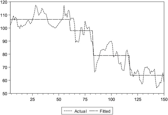
Figure 2.6. US Real Effective Exchange Rate (REER), 1870–2010
Note: Bai–Perron break test result. The red line is the US REER and the green line is best-fitted average.
Another consequence of the devaluation is that it paved the way for more trade integration within Europe. The 1949 devaluation was a necessary condition to open European Payments Union discussions. The Economist noted that ‘every Western European currency, save the Swiss franc, has now made some response to the sterling devaluation’.Footnote 44 Adjusting European currencies against the dollar helped bring trade deficits under control. A year after the devaluation, on 19 September 1950, European nations and the United States put in place the EPU, starting with an initial working capital of $350 million provided by the United States as part of Marshall Aid. The mechanism allowed monthly clearance between European countries, including the sterling area and franc zone. The BIS acted as an agent. The currency of the system was the dollar. Member countries could pay in gold, dollars or EPU credit.Footnote 45


 Open access