


1. Introduction
Characterizing the organization and energy content of coherent structures present in wall-bounded turbulent flows is important for many engineering and environmental pursuits, such as wind energy (Önder & Meyers Reference Önder and Meyers2018), environmental pollutant transport (Reche et al. Reference Reche, D'Orta, Mladenov, Winget and Suttle2018) and urban flows (Barlow Reference Barlow2014). Coherent structures cover a breadth of spatial and temporal scales, including streamwise-aligned packets of hairpin vortices resulting from auto-generation processes, while concatenation processes in the streamwise direction can lead to the generation of structures with a wavelength of the order of 2–3 times the outer scale of turbulence,  $\varDelta _E$ (e.g. the boundary layer thickness), which are denoted as large-scale motions (LSMs) (Adrian Reference Adrian2007; Marusic et al. Reference Marusic, McKeon, Monkewitz, Nagib, Smits and Sreenivasan2010; Smits, McKeon & Marusic Reference Smits, McKeon and Marusic2011; Jiménez Reference Jiménez2018). Even larger structures have been detected with streamwise extent in the range of 8-20
  $\varDelta _E$, denoted as very-large-scale motions (VLSMs) (Kim & Adrian Reference Kim and Adrian1999; Hutchins & Marusic Reference Hutchins and Marusic2007), for which a consensus on their generation process has not been achieved yet (Guala, Hommema & Adrian Reference Guala, Hommema and Adrian2006; Balakumar & Adrian Reference Balakumar and Adrian2007). Very-large-scale motions interact with the near-wall turbulence cycle through nonlinear modulation mechanisms (Mathis, Hutchins & Marusic Reference Mathis, Hutchins and Marusic2009; Talluru et al. Reference Talluru, Baidya, Hutchins and Marusic2014; Lee & Moser Reference Lee and Moser2019; Liu, Wang & Zheng Reference Liu, Wang and Zheng2019; Salesky & Anderson Reference Salesky and Anderson2020).
A cornerstone to achieving an in-depth understanding of the stochastic contribution of coherent structures to the turbulent kinetic energy in wall-bounded flows is the Townsend's attached-eddy hypothesis (AEH) (Townsend Reference Townsend1976), which models the logarithmic layer as a forest of randomly repeated geometrically similar eddies, whose vertical extent,  $\delta$, is proportional to their distance from the wall,
  $z$, and whose eddy population density is inversely proportional to their size. Furthermore, the geometric similarity of wall-attached turbulent motions and the overlapping between inner scaling with
  $z$ and outer scaling with
  $\varDelta _E$ justify the presence of the
  $k_x^{-1}$ region (where
  $k_x$ is the streamwise wavenumber) in the streamwise velocity energy spectrum,
  $\phi _{uu}$ (Perry, Henbest & Chong Reference Perry, Henbest and Chong1986). This spectral feature was also predicted through dimensional analysis (Perry & Abell Reference Perry and Abell1975; Perry et al. Reference Perry, Henbest and Chong1986; Davidson & Krogstad Reference Davidson and Krogstad2009). The spectral extension of this inverse-power-law region is expected to grow with scale separation, and, thus, the friction Reynolds number
  ${\textit {Re}}_\tau =U_\tau \varDelta _E/\nu$, where
  $U_\tau$ is the friction velocity (
 $U_\tau = \sqrt {\tau _0/\rho }$, with
  $\tau _0$ and
  $\rho$ being the wall-shear stress and the fluid density, respectively), and
  $\nu$ the kinematic viscosity. However, evidence of the
  $k_x^{-1}$ spectral region is still elusive even for high
  ${\textit {Re}}_\tau$ laboratory data (Morrison et al. Reference Morrison, Jiang, McKeon and Smits2002; Rosenberg et al. Reference Rosenberg, Hultmark, Vallikivi, Bailey and Smits2013; Vallikivi, Ganapathisubramani & Smits Reference Vallikivi, Ganapathisubramani and Smits2015; Baidya et al. Reference Baidya, Philip, Hutchins, Monty and Marusic2017), and field observations of the atmospheric surface layer (ASL) (Högström, Hunt & Smedman Reference Högström, Hunt and Smedman2002; Calaf et al. Reference Calaf, Hultmark, Oldroyd, Simeonov and Parlange2013).
Perry & Abell (Reference Perry and Abell1977), Perry et al. (Reference Perry, Henbest and Chong1986), Marusic & Perry (Reference Marusic and Perry1995) and Perry & Marusic (Reference Perry and Marusic1995) argued that the coherent structures in wall-bounded flows do not consist of only wall-attached eddies, rather they encompass eddies of different nature. In this scenario, Perry & Marusic (Reference Perry and Marusic1995) reasoned that three different eddy types exist in a wall-bounded flow: wall-attached eddies described by the AEH (type  $\mathcal {A}$ eddies), wall-detached eddies (type
  $\mathcal {B}$ eddies), referring to large-scale structures, superstructures and VLSMs (Högström Reference Högström1990, Reference Högström1992; Högström et al. Reference Högström, Hunt and Smedman2002; Baars & Marusic Reference Baars and Marusic2020a; Hu, Yang & Zheng Reference Hu, Yang and Zheng2020), and Kolmogorov small-scale eddies (type
  $\mathcal {C}$), which dominate the
  $k_x^{-5/3}$ inertial subrange of the streamwise velocity energy spectrum. Despite the capability of the AEH in providing an accurate representation of the stochastic energetic contribution of wall-attached eddies to the logarithmic layer of wall-bounded turbulent flows, the stochastic identification of turbulent coherent structures of different nature, i.e. type
  $\mathcal {A}$,
  $\mathcal {B}$ or
  $\mathcal {C}$ eddies according to the classification proposed by Perry & Marusic (Reference Perry and Marusic1995), is still elusive.
A common technique used to separate the energetic contributions due to coherent structures and, specifically, to isolate the energy connected with wall-attached eddies, is to apply a band-pass filter to the streamwise velocity signals (e.g. Nickels et al. Reference Nickels, Marusic, Hafez and Chong2005; Hwang Reference Hwang2015; Hu et al. Reference Hu, Yang and Zheng2020). The AEH assumes that wall-attached eddies scale as their wall-normal distance, and, thus, the high-wavenumber limit of a band-pass filter aiming at isolating the wall-attached-eddy contribution from the streamwise velocity spectrum should be proportional to  $z$ (Perry & Chong Reference Perry and Chong1982; Meneveau & Marusic Reference Meneveau and Marusic2013; Yang & Meneveau Reference Yang and Meneveau2019; Baars & Marusic Reference Baars and Marusic2020a; Hu et al. Reference Hu, Yang and Zheng2020). Furthermore, the streamwise velocity within the logarithmic layer at a given wall-normal position results from the superposition of contributions induced by wall-attached eddies within the vertical range between
  $z$ and
  $\varDelta _E$. Therefore, the low-frequency limit of a potential band-pass filter should scale with the boundary layer thickness,
  $\varDelta _E$ (Baars & Marusic Reference Baars and Marusic2020a; Hu et al. Reference Hu, Yang and Zheng2020). While there is consensus on the filtering approach to isolate the energetic contribution associated with wall-attached eddies, on the other hand, there are broad discrepancies on the actual spectral limits used for this band-pass filter.
Another technique to separate the energy content associated with coherent structures of different nature was proposed in Baars & Marusic (Reference Baars and Marusic2020a). In their study, the authors generated two spectral filters based on the linear coherence spectrum (LCS) obtained from the streamwise velocity signals collected at a given height and two reference positions, one located in the proximity of the wall and another within the logarithmic layer. Using this data-driven approach, the authors found that the coherence-based low-wavelength limit of the  $k_x^{-1}$ spectral region was proportional to the wall-normal position (
 $\lambda _x\geq 14z$, where
  $\lambda _x$ is the streamwise wavelength), while the high-wavelength limit was proportional to
  $\varDelta _E$.
As mentioned above, the spectral extension of the inverse-power-law region grows with the separation between the outer scale of turbulence,  $\varDelta _E$, and the viscous scale,
  $\nu /U_\tau$. This requirement has spurred the development of experimental facilities (Marusic et al. Reference Marusic, McKeon, Monkewitz, Nagib, Smits and Sreenivasan2010; Smits et al. Reference Smits, McKeon and Marusic2011; Marusic & Monty Reference Marusic and Monty2018) and numerical tools (Jiménez Reference Jiménez2004; Jiménez & Moser Reference Jiménez and Moser2007; Lee & Moser Reference Lee and Moser2015, Reference Lee and Moser2019) enabling investigations of wall-bounded flows at high Reynolds numbers. For the same purpose, the ASL represents a unique opportunity to probe a boundary layer with extremely high Reynolds numbers (Metzger, Mckeon & Holmes Reference Metzger, Mckeon and Holmes2007; Guala, Metzger & McKeon Reference Guala, Metzger and McKeon2011; Hutchins et al. Reference Hutchins, Chauhan, Marusic, Monty and Klewicki2012; Liu, Bo & Liang Reference Liu, Bo and Liang2017; Heisel et al. Reference Heisel, Dasari, Liu, Hong, Coletti and Guala2018; Huang et al. Reference Huang, Brunner, Fu, Kokmanian, Morrison, Perelet, Calaf, Pardyjak and Hultmark2021; Li, Wang & Zheng Reference Li, Wang and Zheng2021) upon filtering out velocity fluctuations connected with non-turbulent scales (Larsén, Vincent & Larsén Reference Larsén, Vincent and Larsen2013; Larsén, Larsén & Petersen Reference Larsén, Larsen and Petersen2016), restricting the data set to subsets presenting negligible effects connected with the atmospheric thermal stratification (Wilson Reference Wilson2008), and strictly verifying the statistical stationarity and convergence of the collected measurements (Metzger et al. Reference Metzger, Mckeon and Holmes2007). Analogies between ASL and laboratory flows have already been investigated for several features of turbulent boundary layers, such as near-wall structures (Klewicki et al. Reference Klewicki, Metzger, Kelner and Thurlow1995), hairpin vortex packets (Hommema & Adrian Reference Hommema and Adrian2003), Reynolds stresses (Kunkel & Marusic Reference Kunkel and Marusic2006; Marusic et al. Reference Marusic, Monty, Hultmark and Smits2013), inclination angle of coherent structures (Liu et al. Reference Liu, Bo and Liang2017), uniform momentum zones (Heisel et al. Reference Heisel, Dasari, Liu, Hong, Coletti and Guala2018), large-scale amplitude modulation process (Liu et al. Reference Liu, Wang and Zheng2019) and LCS (Krug et al. Reference Krug, Baars, Hutchins and Marusic2019; Li et al. Reference Li, Wang and Zheng2021).
Probing ASL flows requires measurement techniques providing sufficient spatio-temporal resolution throughout the ASL thickness. In this realm, wind light detection and ranging (LiDAR) has become a compelling remote sensing technique to investigate atmospheric turbulence. For instance, LiDAR scans can be optimally designed to probe the atmospheric boundary layer and wakes generated by utility-scale wind turbines (e.g. El-Asha, Zhan & Iungo Reference El-Asha, Zhan and Iungo2017; Zhan, Letizia & Iungo Reference Zhan, Letizia and Iungo2020; Letizia, Zhan & Iungo Reference Letizia, Zhan and Iungo2021a,Reference Letizia, Zhan and Iungob). Regarding atmospheric turbulence, LiDAR measurements were used to detect the inverse-power law (Calaf et al. Reference Calaf, Hultmark, Oldroyd, Simeonov and Parlange2013) or the inertial sublayer (Iungo, Wu & Porté-Agel Reference Iungo, Wu and Porté-Agel2013) from the streamwise velocity energy spectra. Multiple simultaneous and co-located LiDAR measurements can be leveraged to measure three-dimensional (3-D) velocity components and Reynolds stresses (Mikkelsen et al. Reference Mikkelsen, Courtney, Antoniou and Mann2008; Mann et al. Reference Mann, Cariou, Courtney, Parmentier, Mikkelsen, Wagner, Lindelöw, Sjöholm and Enevoldsen2009; Carbajo Fuertes, Iungo & Porté-Agel Reference Carbajo Fuertes, Iungo and Porté-Agel2014). More recently, the LiDAR technology was assessed against sonic anemometry during the experimental planetary boundary layer instrumentation assessment (XPIA) campaign showing excellent agreement in probing the horizontal velocity component (Debnath et al. Reference Debnath, Iungo, Ashton, Brewer, Choukulkar, Delgado, Lundquist, Shaw, Wilczak and Wolfe2017a,Reference Debnath, Iungo, Brewer, Choukulkar, Delgado, Gunter, Lundquist, Schroeder, Wilczak and Wolfeb; Lundquist et al. Reference Lundquist2017).
In this work, streamwise velocity measurements collected simultaneously at various wall-normal positions throughout the ASL thickness with a pulsed Doppler scanning wind LiDAR and a sonic anemometer are investigated to identify the spectral boundaries and the maximum vertical extent of the energy contributions associated with wall-attached eddies. The velocity data were collected through fixed scans performed with the azimuth angle of the LiDAR scanning head set along the mean wind direction during near-neutral thermal conditions. After the quantification of the spectral gap and estimation of the outer scale of turbulence,  $\varDelta _E$, the identification of the energy associated with eddies of different nature is performed through two independent methods: first, from the streamwise velocity energy spectra by leveraging the semi-empirical spectral model proposed by Högström et al. (Reference Högström, Hunt and Smedman2002); then, from the LCS obtained between the LiDAR data collected at a reference height and various wall-normal positions, in analogy with the approach proposed by Baars, Hutchins & Marusic (Reference Baars, Hutchins and Marusic2017). Finally, the integrated streamwise energy within both the spectral portion associated with wall-attached eddies, and that due to coherent structures with larger wavelengths, e.g. LSMs, VLSMs and superstructures, is evaluated along the wall-normal direction and assessed against previous laboratory studies.
The remainder of the paper is organized as follows. In § 2 the experimental data set is introduced, while the methodology to analyse the streamwise velocity spectrum and LCS is described in § 3. In § 4 the results on the identification of turbulent coherent structures of different nature and the quantification of their energy content are discussed. Finally, concluding remarks are reported in § 5.
In this work a Cartesian reference frame is used, where  $(x,y,z)$ represent the streamwise, spanwise and wall-normal directions, respectively. The respective mean velocity vector is indicated as
  $\boldsymbol {U}=(U,V,W)$, while the zero-mean velocity fluctuations are
  $\boldsymbol {u}=(u,v,w)$. The overbar denotes the Reynolds average,
  $t$ is time and the superscript ‘
 $+$’ for a dimension of length indicates the viscous scaling with
  $\nu /U_\tau$, while outer scaling is performed via
  $\varDelta _E$.
2. Experimental data set
2.1. The LiDAR field campaign
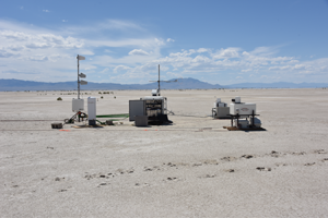
Wind and atmospheric data were collected during the idealized planar array experiment for quantifying surface heterogeneity (IPAQS) campaign performed in June 2018 at the surface layer turbulence and environmental science test (SLTEST) site (Huang et al. Reference Huang, Brunner, Fu, Kokmanian, Morrison, Perelet, Calaf, Pardyjak and Hultmark2021). This site is located in the south–west part of the dry Great Salt Lake, Utah, within the Dugway Proving Ground military facility. The SLTEST site is characterized by an extremely barren and flat ground ( $\approx$1 m elevation difference every 13 km) and exceptionally long unperturbed extensions (
 $\approx$240 km and
  $\approx$48 km in the north–south and east–west directions, respectively) (Kunkel & Marusic Reference Kunkel and Marusic2006). The typical terrain coverage consists of bushes over dry and salty soil, which allow classifying the terrain as transitionally rough (Ligrani & Moffat Reference Ligrani and Moffat1986; Kunkel & Marusic Reference Kunkel and Marusic2006). During the experimental campaign, several instruments were simultaneously deployed for different scientific purposes. The mobile LiDAR station (red triangle in figure 1a) of the University of Texas at Dallas was deployed in the proximity of a 4-by-4 array of CSAT3 3-D sonic anemometers (black circles in figure 1a), manufactured by Campbell Scientific Inc., which recorded the three velocity components and temperature with a sampling frequency of 20 Hz. The sonic-anemometer data considered for this study were collected from the station indicated as ‘PA2’ in figure 1(a) at a 2 m height. The sonic-anemometer data were firstly corrected for pitch and yaw misalignment following the procedure proposed by Wilczak, Oncley & Stage (Reference Wilczak, Oncley and Stage2001), then high-pass filtered as per Hu et al. (Reference Hu, Yang and Zheng2020) with a cutoff frequency
  $\,f_{gap}=0.0055$ Hz, whose selection is discussed in Appendix A.
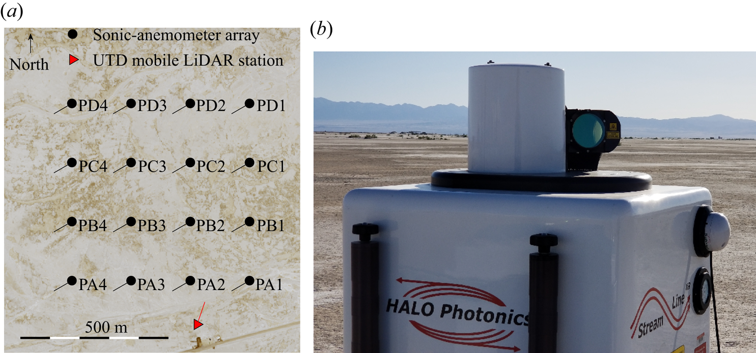
Figure 1. The LiDAR field campaign. (a) Aerial view of the instrument locations. Lines represent the orientation of each instrument, while the labels report the names of each sonic anemometer. (b) Photo of the scanning Doppler wind LiDAR.
To investigate a canonical near-neutral boundary layer, the effects of atmospheric stability on the velocity field should be accounted for. Regarding atmospheric boundary layer flows, the buoyancy contribution to turbulence is compared with the shear-generated turbulence through the Obukhov length,  $L$ (Monin & Obukhov Reference Monin and Obukhov1954),
 \begin{equation} L ={-}\frac{U_{\tau}^3 T}{\kappa g \overline{w\theta}}, \end{equation}
where  $T$ is the mean virtual potential temperature (in Kelvin),
  $\kappa =0.41$ is the von Kármán constant,
  $\overline {w\theta }$ is the vertical heat flux and
  $g$ is the gravity acceleration. Sonic-anemometer data from the PA2 station are further leveraged to calculate the friction velocity according to the eddy-covariance method (Stull Reference Stull1988),
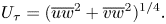 \begin{equation} U_{\tau} = (\overline{uw}^2 + \overline{vw}^2)^{1/4}. \end{equation}
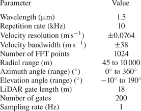
 The pulsed scanning Doppler wind LiDAR deployed for this experiment is a Streamline XR manufactured by Halo Photonics, whose technical specifications are reported in table 1 while a photo of its deployment for the IPAQS field campaign is reported in figure 1(b). A Doppler wind LiDAR allows probing the atmospheric wind field utilizing a laser beam whose light is backscattered due to the presence of particulates suspended in the atmosphere. The velocity component along the laser-beam direction, denoted as radial velocity,  $V_r$, is evaluated from the Doppler shift of the backscattered laser signal (Sathe & Mann Reference Sathe and Mann2013). A pulsed Doppler wind LiDAR emits laser pulses to perform quasi-simultaneous wind measurements at multiple distances from the LiDAR as the pulses travel in the atmosphere. The wind measurements performed over each probe volume, which is referred to as range gate, can be considered as the convolution of the actual wind velocity field projected along the laser-beam direction with a weighting function representing the radial distribution of the energy associated with each laser pulse (Frehlich, Hannon & Henderson Reference Frehlich, Hannon and Henderson1998). Therefore, the radial velocity,
  $V_r$, can be expressed in terms of the instantaneous wind velocity components,
  $(U(t),V(t),W(t))$, where the
  $x$ direction is considered aligned with the mean wind direction,
  $\varTheta _w$, as
 \begin{equation} V_r(t) = U(t)\cos\varTheta\cos\varPhi + V(t)\sin\varTheta\cos\varPhi + W(t)\sin\varPhi, \end{equation}
where  $\varTheta$ is the LiDAR azimuth angle and
  $\varPhi$ is the elevation angle. Both of these angles are measured with a digital inclinometer with an accuracy of 0.005
 $^\circ$ embedded in the LiDAR.
Table 1. Technical specifications of the scanning Doppler wind LiDAR Streamline XR.
To maximize the spatio-temporal resolution of the LiDAR measurements and accuracy in probing the streamwise velocity component, fixed LiDAR scans were performed with a low elevation angle ( $\varPhi =3.5^{\circ }$) and with the laser beam aligned with the mean wind direction, which is monitored by the PA2 sonic anemometer, namely with
  $V\approx 0$ (Iungo et al. Reference Iungo, Wu and Porté-Agel2013). During the post-processing, only LiDAR data sets with an instantaneous deviation of the wind direction smaller than
  ${\pm }10^{\circ }$ from the respective 10 minute average have been considered (Hutchins et al. Reference Hutchins, Chauhan, Marusic, Monty and Klewicki2012). Considering the low elevation angle used and the azimuth angle aligned with the mean wind direction, the first-order approximation for the mean streamwise velocity measured through the wind LiDAR is obtained from (2.3) as
  $U \approx V_r/\cos {\varPhi }$, while for the variance is
  $\overline {uu} \approx \overline {v_rv_r}/\cos ^2{\varPhi }$ (Zhan et al. Reference Zhan, Letizia and Iungo2020).
As previously mentioned, the LiDAR radial velocity is measured through a convolution of the LiDAR laser pulse with the actual velocity field over each range gate. This spatial averaging leads to an underestimation of the measured streamwise turbulence intensity. In this work the streamwise velocity energy spectra, and the respective turbulence intensity obtained as an integral over the measured spectral range, are corrected for the spatial averaging associated with the LiDAR measuring process by using the methodology proposed in Puccioni & Iungo (Reference Puccioni and Iungo2021). For the present set-up, the applied spectral correction only affects the inertial subrange of the streamwise velocity energy spectra calculated for heights larger than the LiDAR range gate (18 m). The reader can refer to Appendix B for more details.
Based on the data quality control described in the following subsection, a subset of one hour of LiDAR data collected during the day of 10 June 2018, from 09:00 AM to 10:00 AM UTC (local time  $-$6 hours) is selected for further analyses, which is characterized by a friction velocity of
  $U_{\tau }=0.42\,\text {m}\,\text {s}^{-1}$, Obukhov length of
  $L=-278$ m, which corresponds to a stability parameter of
  $z/L=-0.007$ indicating a near-neutral atmospheric stability regime (Högström et al. Reference Högström, Hunt and Smedman2002; Kunkel & Marusic Reference Kunkel and Marusic2006; Metzger et al. Reference Metzger, Mckeon and Holmes2007; Mouri, Morinaga & Haginoya Reference Mouri, Morinaga and Haginoya2019; Huang et al. Reference Huang, Brunner, Fu, Kokmanian, Morrison, Perelet, Calaf, Pardyjak and Hultmark2021). For the selected data set, the kinematic viscosity has been estimated
  $\nu =1.49\times 10^{-5}\,\text {m}^2\,\text {s}^{-1}$ based on the mean temperature of
  $290$ K recorded by the sonic anemometer (Picard et al. Reference Picard, Davis, Gläser and Fujii2008).
2.2. Quality control of the LiDAR data
The LiDAR measurements undergo a quality control procedure to ensure the reliability and accuracy of the velocity data. The first parameter used to ensure the accuracy of the LiDAR velocity measurements is the carrier-to-noise ratio (CNR), which represents a quantification of the intensity of the backscattered laser pulse over the typical signal noise as a function of the radial distance and time (Frehlich Reference Frehlich1997; Beck & Kühn Reference Beck and Kühn2017; Gryning & Floors Reference Gryning and Floors2019). For a fixed scan with a constant elevation angle, the range gates selected for any further analysis have a time-averaged CNR not lower than  $-20$ dB (Gryning & Floors Reference Gryning and Floors2019), which corresponds for the selected data set to all the LiDAR measurements collected within the vertical range between 6 and 143 m with a vertical resolution of approximately 1.08 m. Considering an elevation angle of the laser beam of
  $3.5^\circ$, the horizontal range between the first and last LiDAR range gate is then 2246 m.
A filtering procedure is then adopted to remove possible outliers from the LiDAR data, i.e. erroneous estimation of the radial velocity from the backscattered LiDAR signal (Frehlich et al. Reference Frehlich, Hannon and Henderson1998). In this study a standard deviation-based filter is implemented, i.e. any velocity sample out of the interval  $U\pm 3.5 {\overline {uu}}^{1/2}$, which is estimated for the entire 1 h period of the selected data set, is marked as an outlier and removed (Højstrup Reference Højstrup1993; Vickers & Mahrt Reference Vickers and Mahrt1997). The rejected samples are then replaced through a bi-harmonic algorithm with the Matlab function
  $inpaint\_nans$ (D'Errico Reference D'Errico2004). In the worst scenario, the total number of samples rejected for the data collected at a 140-m height is
  $0.75\,\%$ over the 1 h duration of the selected data set. The LiDAR signal quality typically improves by approaching the LiDAR due to the increased energy in the laser beam.
Subsequently, the statistical stationarity of the velocity signals is analysed through the standard deviation dispersion (SDD), which is calculated as (Foken & Wichura Reference Foken and Wichura1996)
 \begin{equation} \text{SDD}=\frac{\sqrt{\langle (\sigma_i-\sigma_0)^2\rangle_i}}{\sigma_0}\times100, \end{equation}
where  $\sigma _0$ is the standard deviation of a velocity signal over its entire sampling period of 1 h, and
  $\sigma _i$ is the velocity standard deviation calculated over a subset with a 5 min duration. The symbol
  $\langle \rangle _i$ indicates the average over the total number of non-overlapping subsets of the original velocity signal. The parameter
  $\textrm {SDD}$ is plotted in figure 2(a) indicating that throughout the vertical range probed by the LiDAR, the statistical stationarity of the velocity signals can be assumed considering a threshold for the
  $\textrm {SDD}$ parameter of
  $30\,\%$ (Foken et al. Reference Foken, Göockede, Mauder, Mahrt, Amiro and Munger2004).
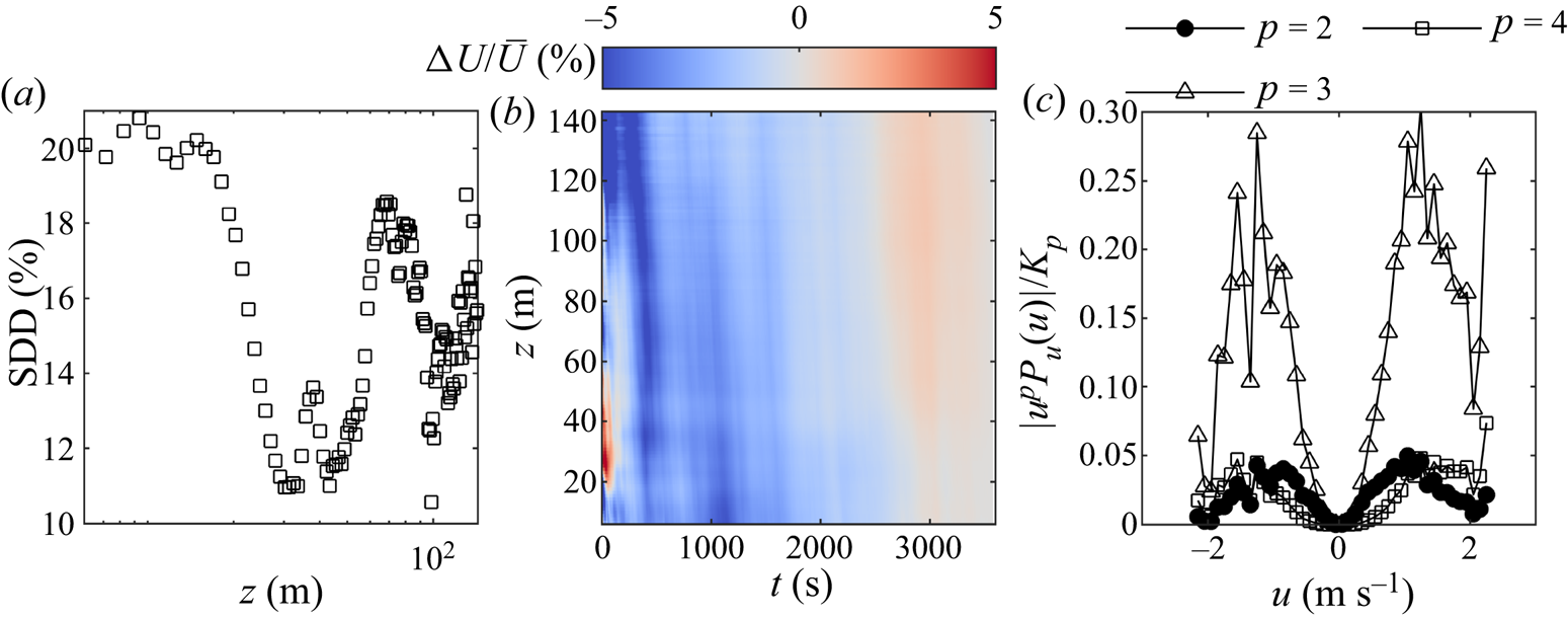
Figure 2. Analysis of the statistical stationarity and convergence of the LiDAR data. (a) The  $\textrm {SDD}$ parameter as a function of height. (b) Percentage difference between cumulative mean for different signal durations,
  $t$, and the mean for the entire 1 h duration of the LiDAR velocity data,
  $\bar {U}$. (c) Normalized absolute value of premultiplied probability density functions for the velocity signal collected at
  $z=143$ m for statistical moments with a different order,
  $p$.
$p$.
The convergence of the mean velocity is then analysed for an increasing number of samples (Heisel et al. Reference Heisel, Dasari, Liu, Hong, Coletti and Guala2018). In figure 2(b) the results of this analysis show that velocity signals with a duration of at least roughly 3000 s are needed to achieve a statistical convergence of the mean value. Furthermore, the statistical convergence of the mean streamwise velocity is comparable among the different heights probed. Finally, the convergence of higher-order statistical moments is qualitatively investigated by inspecting the probability density function of the velocity signal,  $P_u(U)$, for the highest range gate, premultiplied by
  $u^p$, where
  $p$ is the order of the considered central statistical moment. If the tails of the considered function smoothly taper towards zero, then the respective statistical moment,
  $K_p$, can be considered as adequately estimated through the available data (Meneveau & Marusic Reference Meneveau and Marusic2013). For the present study, this analysis is performed considering velocity bins with a width of
  $0.1\,\text {m}\,\text {s}^{-1}$. In figure 2(c) the results suggest a good convergence for the second-order statistics and an incomplete convergence for higher-order statistical moments. The latter is not crucial for the following analyses because higher-order statistics, e.g. skewness and kurtosis, will not be involved.
2.3. Streamwise mean velocity and turbulence intensity
The mean streamwise velocity measured through the wind LiDAR and the PA2 sonic anemometer is scaled with the friction velocity retrieved from the sonic-anemometer data, then compared in figure 3(a) to ASL data collected from previous experiments at different sites with variable terrain roughness (Clarke et al. 1971; Kunkel & Marusic Reference Kunkel and Marusic2006; Tieleman Reference Tieleman2008; Hutchins et al. Reference Hutchins, Chauhan, Marusic, Monty and Klewicki2012; Wang & Zheng Reference Wang and Zheng2016; Heisel et al. Reference Heisel, Dasari, Liu, Hong, Coletti and Guala2018), and laboratory experiments as well (Schultz & Flack Reference Schultz and Flack2007; Squire et al. Reference Squire, Morrill-Winter, Hutchins, Schultz, Klewicki and Marusic2016; Morrill-Winter et al. Reference Morrill-Winter, Squire, Klewicki, Hutchins, Schultz and Marusic2017). For an ASL flow, the effects of the terrain roughness on the mean streamwise velocity can be accounted through the aerodynamic roughness length,  $z_0$, into the logarithmic law of the wall (Kunkel & Marusic Reference Kunkel and Marusic2006; Gryning et al. Reference Gryning, Batchvarova, Brümmer, Jørgensen and Larsén2007; Metzger et al. Reference Metzger, Mckeon and Holmes2007; Heisel et al. Reference Heisel, Dasari, Liu, Hong, Coletti and Guala2018),
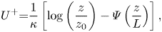 \begin{equation} U^+{=} \frac{1}{\kappa}\left[\log \left(\frac{z}{z_0}\right) - \varPsi\left(\frac{z}{L} \right) \right], \end{equation}
where  $\varPsi$ is the stability correction function (Businger et al. Reference Businger, Wyngaard, Izumi and Bradley1971). The experimental data are fitted with (2.5) to estimate the aerodynamic roughness length, which results in
  $z_0=8.71\times 10^{-6}$ m. By normalizing the wall-normal position with
  $z_0$, a very good agreement is observed in figure 3(b) between the stability-corrected mean streamwise velocity measured by the LiDAR and previous data sets. Furthermore, (2.5) is used to assess the value of
  $U_\tau$ calibrated on the LiDAR data (
 $U_\tau =0.51\pm 0.009$ m s
 $^{-1}$) against that estimated from the sonic-anemometer data using the eddy-covariance method (
 $U_\tau =0.42$ m s
 $^{-1}$).
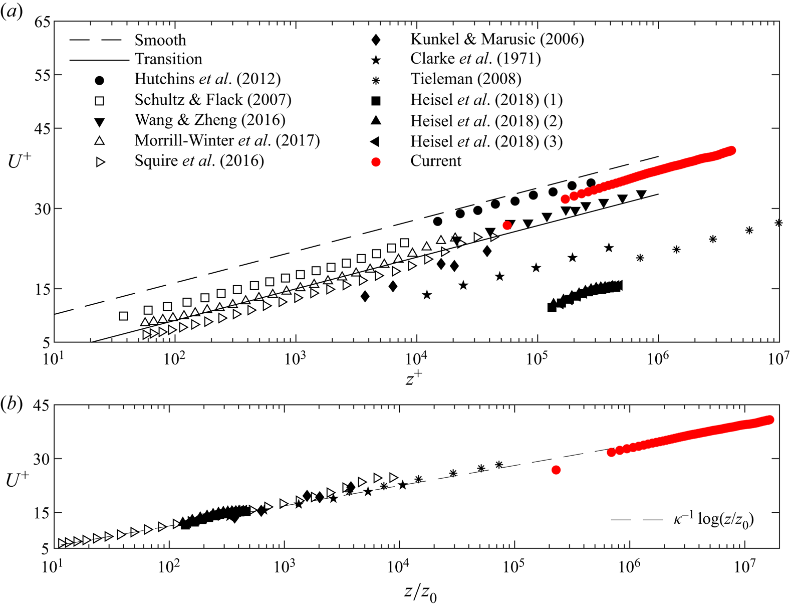
Figure 3. Mean streamwise velocity measured from the LiDAR and the PA2 sonic anemometer (the lowest point). (a) Mean velocity versus inner-scaled wall-normal coordinate. (b) Wall-normal coordinate is made non-dimensional with the aerodynamic roughness length,  $z_0$. Empty and filled symbols refer to wind tunnel and ASL studies, respectively. This figure is adapted from Heisel et al. (Reference Heisel, Dasari, Liu, Hong, Coletti and Guala2018).
Another way to account for the terrain roughness on the mean streamwise velocity profile is through the sand-grain roughness parameter,  $k_s^+$,
 \begin{equation} U^+{=} \frac{1}{\kappa}\log\left(\frac{z^+}{k_s^+} \right)+B(k_s^+), \end{equation}
where  $B(k_s^+)$ is a function accounting for the vertical shift of the mean velocity profile. For a transitional roughness regime, where
  $2.25\leq k_s^+\leq 90$ (Ligrani & Moffat Reference Ligrani and Moffat1986; Hutchins et al. Reference Hutchins, Chauhan, Marusic, Monty and Klewicki2012),
  $B(k_s^+)$ is given by (Kunkel & Marusic Reference Kunkel and Marusic2006)
 \begin{equation} B(k_s^+) = \frac{1}{\kappa}\log k_s^+{+} 5.0 + \sin\left(\frac{{\rm \pi} h}{2} \right)\left(8.5-5.0-\frac{1}{\kappa}\log k_s^+ \right), \end{equation}
where
 \begin{equation} h = \frac{\log(k_s^+{/}90)}{\log(k_s^+{/}2.25)}. \end{equation}
Comparing (2.5) and (2.6), the sand-grain roughness can be estimated from  $z_0$ as
  $k_s^+ = 11.4$ (
 $k_s=0.41$ mm), which is of the same order of magnitude as for previous estimates for the SLTEST site, e.g.
  $k_s^+\approx 34$ (
 $k_s=2.9$ mm) in Kunkel & Marusic (Reference Kunkel and Marusic2006), or
  $k_s^+=15$ in Huang et al. (Reference Huang, Brunner, Fu, Kokmanian, Morrison, Perelet, Calaf, Pardyjak and Hultmark2021).
The inner-scaled wall-normal profile of the turbulence intensity is reported against the viscous- and outer-scaled wall-normal coordinate in figure 4(a,b), respectively. The estimate of the outer scale of turbulence,  $\varDelta _E=127$ m for the present data set, is detailed in Appendix A. Based on the AEH, the law for the wall-normal distribution of streamwise turbulence intensity can be written as (Townsend Reference Townsend1976; Perry & Chong Reference Perry and Chong1982)
 \begin{equation} {\overline{uu}^+}=B_1-A_1\log\left(\frac{z}{\varDelta_E}\right), \end{equation}
where  $B_1$ is a flow-dependent constant accounting for the large-scale inactive motion, while
  $A_1$ is the Townsend–Perry constant (Perry et al. Reference Perry, Henbest and Chong1986; Baars & Marusic Reference Baars and Marusic2020b). For the SLTEST site under neutral conditions, Marusic et al. (Reference Marusic, Monty, Hultmark and Smits2013) reported that
  $A_1=1.33\pm 0.17$ and
  $B_1=2.14\pm 0.40$, whereas for the current data set we obtain
  $A_1=1.11\pm 0.04$ and
  $B_1=1.43\pm 0.05$.
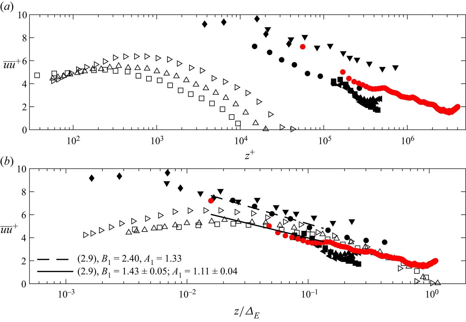
Figure 4. Wall-normal profile of turbulence intensity with the (a) inner-scaled and (b) outer-scaled wall-normal coordinate. For the current data set, the lowest point is retrieved from the PA2 sonic anemometer. In (b) the black continuous line refers to the model of Marusic et al. (Reference Marusic, Monty, Hultmark and Smits2013) calibrated on the present data set. Legend as for figure 3. This figure is adapted from Heisel et al. (Reference Heisel, Dasari, Liu, Hong, Coletti and Guala2018).
3. Contribution of eddies with different typology to the streamwise velocity energy
3.1. Reynolds stresses and isolated-eddy function
According to the AEH, a wall-attached eddy has a wall-normal extent,  $\delta$, growing linearly with the distance from the wall,
  $z$ (Townsend Reference Townsend1976; Perry & Chong Reference Perry and Chong1982). Therefore, the probability density function representing the occurrence of an eddy with size
  $\delta$,
  $p_H(\delta )$, should decrease monotonically with
  $z$ (Townsend Reference Townsend1976),
 \begin{equation} p_H(\delta) = \left\{\begin{array}{@{}ll@{}} \dfrac{M}{\delta} & \textrm{as}\ \delta_1\leq\delta\leq\varDelta_E, \\ 0 & \textrm{otherwise}, \end{array}\right. \end{equation}
where  $M$ is a constant related to the eddy population density on the plane of the wall (De Silva, Hutchins & Marusic Reference De Silva, Hutchins and Marusic2015), and
  $\delta _1\approx 100\nu /U_{\tau }$ is the smallest eddy size owning to the logarithmic layer, which is fixed by the viscous cutoff (Kline et al. Reference Kline, Reynolds, Schraub and Runstadler1967; Perry & Chong Reference Perry and Chong1982). The Reynolds stresses at a given
  $z$ are then calculated as the weighted integral of isolated-eddy contributions over the entire scale range,
 \begin{equation} \overline{u_iu_j}^+{=}\int_{\delta_1}^{\varDelta_E}I_{ij} \left(\frac{z}{\delta}\right)p_H(\delta)\,\text{d}\delta= \int_{\delta_1}^{\varDelta_E}MI_{ij}\left(\frac{z}{\delta}\right) \frac{\text{d}\delta}{\delta} = \int_{z/\varDelta_E}^{z/\delta_1}MI_{ij} \left(\frac{z}{\delta} \right)\frac{\delta}{z} \text{d}\left(\frac{z}{\delta}\right), \end{equation}
where the function  $I_{ij}$ is referred to as the ‘eddy function’, representing the geometrically self-similar isolated-eddy contribution to
  $\overline {u_iu_j}^+$. In the view of the AEH,
  $I_{ij}$ is determined by the sole geometrical features of the archetypal wall-attached eddy. Remarkably,
  $I_{ij}$ can also be estimated for a fixed eddy size,
  $\delta$, through the differential form of (3.2),
 \begin{equation} I_{ij}\left(\frac{z}{\delta} \right)={-}\frac{z}{M} \frac{\partial \overline{u_i u_j}^+}{\partial z}. \end{equation}
The term on the right-hand side of (3.3) is commonly referred to as the ‘indicator function’ and it has been used to detect the presence and extent of the logarithmic region (e.g. Bernardini, Pirozzoli & Orlandi Reference Bernardini, Pirozzoli and Orlandi2014; Lee & Moser Reference Lee and Moser2015; Hwang & Sung Reference Hwang and Sung2018; Yamamoto & Tsuji Reference Yamamoto and Tsuji2018; Klewicki Reference Klewicki2021). It is noteworthy that (3.3) represents the contribution to the Reynolds stresses of the sole wall-attached eddies (type  $\mathcal {A}$), and, thus, does not encompass the contribution of wall-detached eddies, or coherent structures characterized by larger wavelengths, e.g. VLSMs and superstructures (type
  $\mathcal {B}$).
3.2. Regions of the streamwise velocity energy spectrum
Regarding the streamwise velocity spectrum, as mentioned in § 1, for wall-normal locations owning to the inertial layer, the non-dimensional low-wavenumber limit of the  $k_x^{-1}$ region (denoted as
  $F$ following the notation of Perry et al. Reference Perry, Henbest and Chong1986) scales with
  $\varDelta _E$ (Perry & Chong Reference Perry and Chong1982; Perry et al. Reference Perry, Henbest and Chong1986). Therefore, the large eddies with scale
  $O(\varDelta _E)$ will contribute to the streamwise velocity energy spectrum as
 \begin{equation} \phi_{uu}^+(k_x\varDelta_E) = g_1(k_x\varDelta_E) = \frac{\phi_{uu}(k_x)}{\varDelta_EU_\tau^2}. \end{equation}
On the other hand, the non-dimensional high-wavenumber limit of the inverse-power-law spectral region,  $P$, scales with
  $z$, and the respective eddies contribute to the streamwise velocity energy spectrum as
 \begin{equation} \phi_{uu}^+(k_xz) = g_2(k_xz) = \frac{\phi_{uu}(k_x)}{zU_\tau^2}. \end{equation}
Considering an overlapping region where (3.4) and (3.5) hold simultaneously, and, thus, equating  $\phi _{uu}(k_x)$ from (3.4) and (3.5), we obtain
 \begin{equation} \frac{g_1(k_x\varDelta_E)}{g_2(k_xz)}= \frac{z}{\varDelta_E}. \end{equation}
Therefore, within this overlapping region,  $g_1$ and
  $g_2$ must be of the form (Perry & Abell Reference Perry and Abell1975; Perry et al. Reference Perry, Henbest and Chong1986; Davidson & Krogstad Reference Davidson and Krogstad2009)
 \begin{equation} g_1(k_x\varDelta_E) = \frac{A_1}{k_x\varDelta_E};\quad g_2(k_xz) = \frac{A_1}{k_xz},\end{equation}
where  $A_1$ is the Townsend–Perry constant, which is of the order of
  $1$ (Perry et al. Reference Perry, Henbest and Chong1986; Baars & Marusic Reference Baars and Marusic2020b). The turbulence intensity associated with wall-attached eddies is then expressed as the integral of the streamwise velocity energy spectrum over the different regions, i.e.
 \begin{equation} \overline{uu}^+{=} \int_0^{F} g_1(k_x\varDelta_E)\,\text{d}(k_x\varDelta_E) + \int_{Fz/\varDelta_E}^P g_2(k_xz)\,\text{d}(k_xz) + \int_{P}^\infty \phi_{uu}^+(k_xz)\,\text{d}(k_xz). \end{equation}
A similar approach for the identification of different regions of the streamwise velocity energy spectrum was proposed by Högström et al. (Reference Högström, Hunt and Smedman2002) for ASL flows. Specifically, three different regions are singled out within the turbulence spectral range by this model, which are indicated with dashed lines in the sketch reported in figure 5. Region (i) is the inertial subrange, which follows the Kolmogorov law
 \begin{equation} k_x^+\phi_{uu}^+ (k_x)= \frac{\alpha_K}{(2{\rm \pi}\kappa)^{2/3}}\varphi_{\varepsilon}^{2/3} \left(\frac{k_xz}{2{\rm \pi}} \right)^{{-}2/3}, \end{equation}
where  $\alpha _K$ is the Kolmogorov constant,
  $\kappa$ is the von Kármán constant and
  $\varphi _{\varepsilon }$ is the non-dimensional dissipation rate, which can be estimated as follows (Kaimal et al. Reference Kaimal, Wyngaard, Izumi and Coté1972):
 \begin{equation} \varphi_\varepsilon^{2/3}\left(\frac{z}{L}\right)= \left(\frac{\kappa z \varepsilon}{U_\tau^3}\right)^{2/3}=\left\{\begin{array}{@{}ll} 1+0.5\left|\dfrac{z}{L} \right|^{2/3}, & -2\leq z/L\leq0, \\ 1+2.5\left|\dfrac{z}{L} \right|^{3/5}, & 0\leq z/L\leq2. \end{array}\right. \end{equation}
Here  $\varepsilon$ is the turbulent kinetic energy dissipation rate and
  $L$ is the Obukhov length (see § 2.1). It is noted that the maximum value attained by the stability correction function in (3.10) is equal to 1.32 at
  $z=143$ m for the data set under investigation.
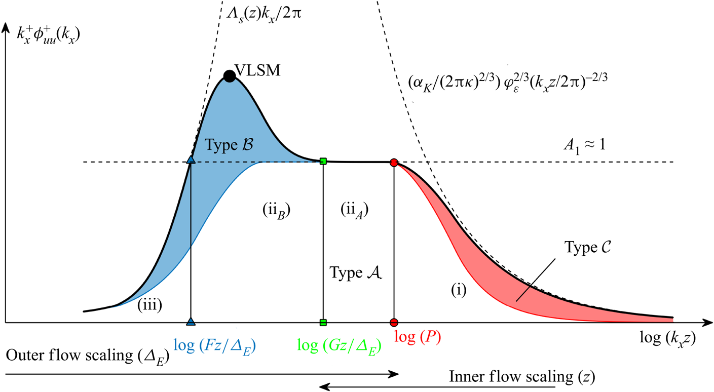
Figure 5. Sketch of the different regions encompassed in the streamwise velocity premultiplied energy spectrum.
Region (ii) corresponds to the spectral range where the premultiplied spectrum is nearly constant,
 \begin{equation} k_x^+\phi_{uu}^+ (k_x)\approx A_1, \end{equation}
where  $A_1$ is the Townsend–Perry constant in (2.9). The wall-normal range where region (ii) was observed in the ASL, which is dubbed the ‘eddy surface layer’ (ESL), has a thickness of about
  $\varDelta _E/3$ (Hunt & Morrison Reference Hunt and Morrison2000; Högström et al. Reference Högström, Hunt and Smedman2002). This estimate is similar to that for the height of the logarithmic layer for ASL flows reported in Hutchins et al. (Reference Hutchins, Chauhan, Marusic, Monty and Klewicki2012), while Marusic et al. (Reference Marusic, Monty, Hultmark and Smits2013) conservatively quantified the height of the logarithmic layer based on mean velocity profiles and turbulence intensity at
  $z=0.15\varDelta _E$ for laboratory flows.
For region (iii), the premultiplied spectrum increases with the wavenumber,
 \begin{equation} k_x^+\phi_{uu}^+ (k_x)= \varLambda_s \frac{k_x}{2{\rm \pi}}. \end{equation}
The parameter  $\varLambda _s$ is a large-scale characteristic wavelength estimated as
  $\varLambda _s=A(z)U_\tau /f_C$, where
  $f_C$ is the Coriolis frequency (Rossby & Montgomery Reference Rossby and Montgomery1935) (
 $f_C=9.38\times 10^{-5}$ Hz for the present data set), the parameter
  $A$ is linearly proportional to
  $z$ within the ESL, while
  $\varLambda _s$ reaches the maximum value at the height of the ESL, then decreases (Högström et al. Reference Högström, Hunt and Smedman2002).
The model of Högström et al. (Reference Högström, Hunt and Smedman2002) defined through (3.9), (3.11) and (3.12) allows for calculating the boundaries of region (ii). Specifically, from  $A(z)$ and
  $A_1$, the non-dimensional low-wavenumber limit of region (ii),
  $F$, can be found by equating (3.11) and (3.12),
 \begin{equation} F=\frac{2{\rm \pi} f_CA_1\varDelta_E}{A(z)U_\tau}. \end{equation}
Similarly, the wavenumber at the intersection between regions (i) and (ii) is found by equating (3.9) and (3.11),
 \begin{equation} P=\frac{1}{\kappa}\left(\frac{\alpha_K\varphi_\varepsilon^{2/3}}{A_1} \right)^{3/2}. \end{equation}
 Building upon the spectral model proposed by Högström et al. (Reference Högström, Hunt and Smedman2002), we propose to further divide region (ii) into two high- and low-wavenumber sub-regions referred to as (ii $_A$) and (ii
 $_B$), respectively, where the energy contribution of wall-attached eddies (type-
 $\mathcal {A}$ eddies) is predominant for the former, while that associated with type-
 $\mathcal {B}$ eddies is predominant for the latter (see figure 5). This approach is inspired by previous works; for instance, Rosenberg et al. (Reference Rosenberg, Hultmark, Vallikivi, Bailey and Smits2013) and Vallikivi et al. (Reference Vallikivi, Ganapathisubramani and Smits2015) modelled separately the VLSM spectral peak through a Gaussian function (here associated with region (ii
 $_B$)) and the flat premultiplied region through a cubic spline. For our study, the non-dimensional wavenumber at the intersection between regions (ii
 $_A$) and (ii
 $_B$), indicated with
  $G$ in figure 5, is thought to scale with
  $\varDelta _E$ considering that its spectral value is affected by the energy content of type-
 $\mathcal {B}$ eddies, which scale with
  $\varDelta _E$. Finally, the maximum height where region (ii
 $_A$) can be observed,
  $z_{max}$, is identified where the condition
  $P=z_{max}G/ \varDelta _E$ is fulfilled.
The technical strategy for the quantification of  $F,G$, and
  $P$ from the premultiplied streamwise velocity spectrum is detailed in the following. Starting from region (i), the term
  $\alpha _K/\kappa ^{2/3}$ in (3.9) is fitted by overlapping the premultiplied streamwise velocity spectra versus the inertia-scaled wavenumber for all the heights probed by the LiDAR and over the frequency range
  $k_xz\geq 2$. The fitting of the experimental spectra leads to an estimate of
  $\alpha _K/\kappa ^{2/3}=0.60$ for the present data set.
For region (ii $_A$),
  $A_1$ is heuristically determined for each height in the proximity of the spectral range where the high-frequency limit
  $P$ is expected (
 $k_xz\approx 1$). Subsequently, the intersection between the horizontal line equal to
  $A_1$ and the fitted spectrum for region (i) leads to the identification of the high-wavenumber limit
  $P$.
$P$.
For region (iii),  $A(z)$ is obtained for each height through the fitting of the streamwise velocity energy spectra with (3.12) limited to the low-frequency energy-increasing portion. Then, for each height, the intersection between the horizontal line equal to
  $A_1$ and the fitted spectrum for region (iii) identifies the low-frequency limit
  $F$. Finally, the inner boundary between regions (ii
 $_A$) and (ii
 $_B$),
  $G$, is heuristically quantified at the crossing between the energy-decreasing region for smaller wavenumbers typically associated with VLSMs and the horizontal line equal to
  $A_1$.
3.3. Identification of the energy associated with different eddy typology based on the LCS of the streamwise velocity
The scale-dependent cross-correlation of two statistically stationary velocity signals collected at wall-normal positions  $z$ and
  $z_R$ (reference height) can be estimated through the two-point LCS,
 \begin{equation} \gamma^2(z,z_R;k_x) = \frac{|\phi_{uu}'(z,z_R;k_x)|^2}{\phi_{uu}(z;k_x) \phi_{uu}(z_R;k_x)}, \end{equation}
where  $||$ indicates the modulus while
  $\phi _{uu}'(z,z_R;k_x)$ is the cross-spectral density of the two streamwise velocity signals, which is practically the Fourier transform of the cross-variance function between
  $u(z)$ and
  $u(z_R)$. Therefore, the LCS represents the fraction of common variance shared by
  $u(z_R)$ and
  $u(z)$ across frequencies (Bendat & Piersol Reference Bendat and Piersol1986). Due to the normalization with the single-point energy spectra, we have
  $0\leq \gamma ^2\leq 1$. Considering that the LCS is calculated from the amplitude of the cross-spectral density, no information is retained about the phase shift of the shared energy between the two velocity signals (Nelson, Hati & Howe Reference Nelson, Hati and Howe2013; Baars et al. Reference Baars, Hutchins and Marusic2017). This feature is advantageous when calculating the LCS from the LiDAR data, which are collected with a streamwise shift of about 18 m between consecutive LiDAR gates due to the elevation angle of 3.5
 $^\circ$ set for the LiDAR fixed scans. Nonetheless, it is reasonable to expect a slight reduction of
  $\gamma ^2$ for a large height difference between
  $z_R$ and
  $z$ associated with the limitations in the applicability of the Taylor's hypothesis of frozen turbulence (Taylor Reference Taylor1938).
Considering a boundary layer flow encompassing only wall-attached eddies generated by a single hierarchy with wavelength  $\lambda _H$, vertical size
  $\delta$, and, thus, aspect ratio
  ${A{\kern-4pt}R} = \lambda _H / \delta$, the non-zero portion of the LCS is limited to wall-normal positions with
  $z\leq \delta$, since no wall-attached eddies are present above, and to wavelengths with
  $\lambda _x\geq \lambda _H={A{\kern-4pt}R} \delta$ due to the concatenation and random repetitions of the same hierarchy along the streamwise direction (Baars et al. Reference Baars, Hutchins and Marusic2017). Therefore, the isolated-eddy contribution to the LCS for a single hierarchy can be modelled as
 \begin{equation} \gamma_{H}^2 \left(\frac{\lambda_x}{\delta},\frac{z}{\delta}\right) = C_0 H \left[1-\frac{z}{\delta} \right]H \left[\frac{\lambda_x}{{A{\kern-4pt}R}\delta}-1 \right];\quad \text{as}\ \frac{z}{\delta}\leq 1,\enspace \dfrac{\lambda_x}{{A{\kern-4pt}R}\delta}\geq 1, \end{equation}
where  $H$ is the unit Heaviside function, while the parameter
  $C_0$ (
 $0< C_0<1$) represents the isolated-eddy contribution to the LCS, and it only depends on the geometric features of the archetypal eddy. When a continuous distribution of attached eddies is considered, the resulting LCS will then be expressed as the sum of the various isolated contributions weighted by their probability density function throughout the scale range
 \begin{equation} \gamma^2\left(\frac{\lambda_x}{\varDelta_E};\frac{z}{\delta_{min}}, \frac{z}{\varDelta_E} \right) = \min\left[\int_{\delta_{min}}^{\varDelta_E}M\gamma_{H}^2 \left(\frac{\lambda_x}{\delta},\frac{z}{\delta} \right) \frac{\text{d}\delta}{\delta},1\right], \end{equation}
where  $\delta _{min}$ is equal to
  $\delta _1$ or
  $z_R$ if the latter is located in the near-wall or logarithmic region, respectively. Considering that
 \begin{equation} H\left[\frac{\lambda_x}{{A{\kern-4pt}R}\delta }-1 \right] = H\left[\frac{z}{\delta}-\frac{{A{\kern-4pt}R} z}{\lambda_x} \right], \end{equation}
(3.17) becomes
 \begin{equation} \gamma^2\left(\frac{\lambda_x}{\varDelta_E};\frac{z}{\delta_{min}}, \frac{z}{\varDelta_E} \right) = \min\left\{\int_{z/\varDelta_E}^{z/\delta_{min}}C_1 H \left[1-\frac{z}{\delta} \right]H\left[\frac{z}{\delta}-\frac{{A{\kern-4pt}R} z}{\lambda_x} \right] \frac{\delta}{z}\text{d}\left(\frac{z}{\delta} \right),1\right\}, \end{equation}
where  $C_1=MC_0$. Therefore, for a certain
  $z$ and
  $\lambda _x$, the region where the contribution to the LCS is non-zero depends on the values of
  $\varDelta _E,\delta _{min}$ and
  ${A{\kern-4pt}R}$. Specifically, four combinations are possible among these limits, each of them schematically reported in figure 6. For instance, assuming a wall-normal location within the logarithmic region (
 $z\geq \delta _1$) and
  ${A{\kern-4pt}R} z\leq \lambda _x\leq {A{\kern-4pt}R} \varDelta _E$, the case reported in figure 6(a) is obtained, where the active boundaries of the non-zero contribution to the LCS are
  ${A{\kern-4pt}R} z/\lambda _x$ and
  $1$. Thus, (3.19) becomes
 \begin{equation} \gamma^2=\min\left\{\int_{{A{\kern-4pt}R} z/\lambda_x}^{1}C_1 \frac{\delta}{z} \text{d}\left( \dfrac{z}{\delta}\right),1\right\} = \min\left\{C_1\log\left(\frac{\lambda_x}{{A{\kern-4pt}R} z} \right),1\right\}, \end{equation}
which is the model proposed by Baars et al. (Reference Baars, Hutchins and Marusic2017). This case, together with the three remaining combinations between active boundaries of (3.19) (sketched in figure 6b–d), lead to the analytical formulation of the LCS for an attached-eddy flow.
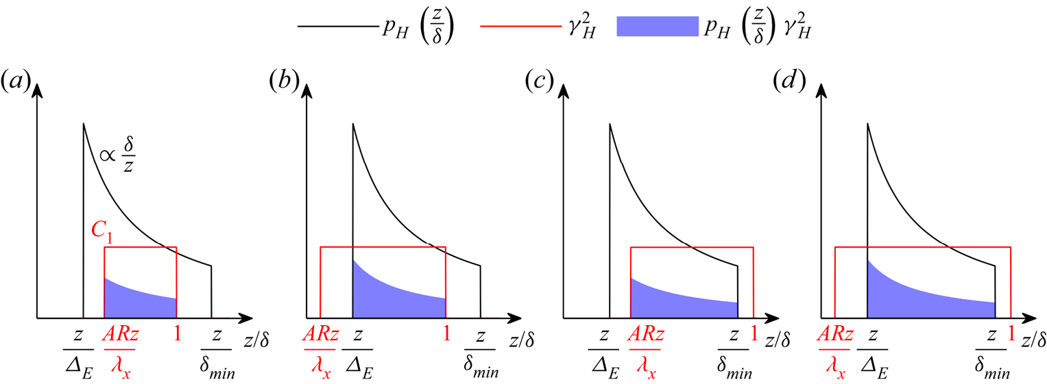
Figure 6. Isolated-eddy contribution to the LCS,  $\gamma _H^2$ (3.16), p.d.f. of an isolated eddy with vertical extent
  $\delta$,
  $p_H$, and their product for the various combinations of
  $\varDelta _E,\delta _{min}$ and
  ${A{\kern-4pt}R}$. The various functions reported on the vertical axis are listed in the legend.
In Baars et al. (Reference Baars, Hutchins and Marusic2017) it was noted that the LCS becomes zero for heights below  $\varDelta _E$. To encompass this feature, an offset for
  $\gamma ^2$, denoted as
  $C_3$, is added to the analytical formulation of the LCS model developed from (3.19), which then reads as
 \begin{align} \gamma^2 = \left\{\begin{array}{@{}ll@{}} \min\left[C_1\log \left(\dfrac{\lambda_x}{{A{\kern-4pt}R} z} \right),1\right] & \text{if}\ z\geq z_R,\enspace \lambda_x/\varDelta_E \leq \exp\left(\dfrac{C_3}{C_1}\right){A{\kern-4pt}R}\ (a), \\ \min\left[{-}C_1\log \left(\dfrac{z}{\varDelta_E} \right)+C_3,1\right] & \text{if}\ z\geq z_R,\enspace \lambda_x/\varDelta_E> \exp\left(\dfrac{C_3}{C_1}\right){A{\kern-4pt}R}\ (b), \\ \min\left[C_1\log \left(\dfrac{\lambda_x}{{A{\kern-4pt}R}\delta_{min}} \right),1\right] & \text{if}\ z< z_R,\enspace \lambda_x/\varDelta_E\leq \exp\left(\dfrac{C_3}{C_1}\right){A{\kern-4pt}R}\ (c), \\ \min\left[C_1\log \left(\dfrac{\varDelta_E}{\delta_{min}} \right)+C_3,1\right] & \text{if}\ z< z_R,\enspace \lambda_x/\varDelta_E> \exp\left(\dfrac{C_3}{C_1}\right){A{\kern-4pt}R}\ (d). \end{array}\right. \end{align}
The threshold wavelength  $\lambda _x^{th}/\varDelta _E = \exp (C_3/C_1){A{\kern-4pt}R}$ is obtained enforcing continuity in
  $\lambda _x$ between (3.21a) and (3.21b), and it represents the boundary between wall-attached eddies and coherent structures generated from their streamwise concatenation. It is noteworthy that including
  $C_3$ implies
  $\gamma ^2=0$ at
  $z_{max}/\varDelta _E=\exp (C_3/C_1)$, rather than at
  $z/\varDelta _E=1$. In Baars et al. (Reference Baars, Hutchins and Marusic2017),
  $\gamma ^2=0$ was identified for
  $z\gtrapprox 0.7\varDelta _E$ while the authors estimated
  $C_1=0.302$, which leads to
  $C_3=-0.103$.
All the cases in (3.21) were observed experimentally in Baars & Marusic (Reference Baars and Marusic2020a), and it is shown here that they are consistent with a continuous distribution of wall-attached eddies. In particular, assuming  $z_R$ within the near-wall region, we have
  $\delta _{min}=\delta _1$ and (3.21) becomes (4.7) of Baars & Marusic (Reference Baars and Marusic2020a). Similarly, assuming
  $z_R$ within the logarithmic region we have
  $\delta _{min}=z_R$, which leads to (4.10) of Baars & Marusic (Reference Baars and Marusic2020a).
It is noteworthy that in Baars & Marusic (Reference Baars and Marusic2020a),  $C_1$ and
  ${A{\kern-4pt}R}$ are calibrated twice from the experimental distribution of LCS depending on whether the reference height was located in the near-wall or logarithmic region. Specifically, it was estimated
  $C_1=0.302$ and
  ${A{\kern-4pt}R} =14.01$ if
  $z_R$ resides in the near-wall region and
  $C_1=0.383$ and
  ${A{\kern-4pt}R} =13.18$ if
  $z_R$ resides in the logarithmic region. This discrepancy is attributed by Baars & Marusic (Reference Baars and Marusic2020a) to the use of a single convection velocity for the application of the Taylor's hypothesis for frozen turbulence. From the proposed LCS model, we confirm that
  $C_1$ should not change with the reference height assuming a constant
  ${A{\kern-4pt}R}$.
3.4. Notes on the LCS of the streamwise velocity
By considering the logarithmic coordinates  $\lambda ^*=\log (\lambda _x/\varDelta _E)$ and
  $z^*=\log (z/\varDelta _E)$, the LCS model of (3.21) can be rewritten, by only considering the case with
  $\gamma ^2\leq 1$, as
 \begin{equation} \gamma^2 = \left\{\begin{array}{@{}ll} C_1\left(\lambda^*-\lambda^*_{th}\right) -C_1 \left({\rm \Delta} z^* + z^*_R \right) +C_3 & \text{if}\ {\rm \Delta} z^*\geq 0,\enspace \lambda^* \leq \lambda^*_{th}\ (a), \\ -C_1 \left({\rm \Delta} z^* + z^*_R \right) +C_3 & \text{if}\ {\rm \Delta} z^*\geq 0,\enspace \lambda^* > \lambda^*_{th}\ (b), \\ C_1\left(\lambda^*-\lambda^*_{th}\right) -C_1 z^*_R +C_3 & \text{if}\ {\rm \Delta} z^*< 0,\enspace \lambda^* \leq \lambda^*_{th}\ (c), \\ -C_1 z^*_R +C_3 & \text{if}\ {\rm \Delta} z^*< 0,\enspace \lambda^* > \lambda^*_{th}\ (d), \end{array}\right. \end{equation}
where  $\lambda ^*_{th}=C_3/C_1+\log ({A{\kern-4pt}R} )$ and
  ${\rm \Delta} z^*=\log (z/z_R)$. Based on (3.22), the following considerations can be made.
(a) For
 $\lambda ^* \leq \lambda ^*_{th}$, $\gamma ^2$ is a linear function of $\lambda ^*$, its slope is not a function of $z^*$ and has a constant value equal to $C_1$.
(b) For
$\lambda ^* > \lambda ^*_{th}$, $\gamma ^2$ achieves an asymptotic value, $\gamma _\infty ^2$, which is a linear function of ${\rm \Delta} z^*$ with slope $-C_1$ if ${\rm \Delta} z^*\geq 0$ while it is constant for ${\rm \Delta} z^*<0$.(c) The threshold wavelength,
$\lambda ^*_{th}$, is not a function of $z^*$.(d) The intercept of
$\gamma ^2$ for $\lambda ^* \leq \lambda ^*_{th}$ is equal to the asymptotic value achieved for $\lambda ^* > \lambda ^*_{th}$ for every $z^*$.


By imposing  $\gamma ^2=0$ in (3.21), we obtain the boundary conditions for a non-null LCS,
 \begin{equation} \left\{\begin{array}{@{}ll@{}} z^*=\lambda^*-\log({A{\kern-4pt}R}) & \text{if}\ {\rm \Delta} z^*\geq 0,\enspace \lambda^* \leq \lambda^*_{th}\ (a), \\ z^*=C_3/C_1 & \text{if}\ {\rm \Delta} z^*\geq 0,\enspace \lambda^* > \lambda^*_{th}\ (b), \\ \lambda^*=z_R^*+\log({A{\kern-4pt}R}) & \text{if}\ {\rm \Delta} z^*< 0,\enspace \lambda^* \leq \lambda^*_{th}\ (c), \\ z_R^*=C_3/C_1 & \text{if}\ {\rm \Delta} z^*< 0,\enspace \lambda^* > \lambda^*_{th}\ (d). \end{array}\right. \end{equation}
The relationship (3.23a) represents the line separating the coherent from the non-coherent component of the flow with  $z_R$ in the (
 $\lambda _x$,
  $z$) domain. According to the LCS model, this line represents the spectral boundary between region (i) and region (ii
 $_A$) for wall-normal positions above
  $z_R$. Below
  $z_R$, the zero contour of
  $\gamma ^2$ has a constant value of
  $\lambda _x$ (3.23c) because, according to the AEH, eddies with a height smaller than
  $z_R$ do not contribute to the LCS. It is noteworthy that the spectral boundary between region (i) and region (ii
 $_A$) is only a function of
  ${A{\kern-4pt}R}$, and it shifts towards larger wavelengths as
  ${A{\kern-4pt}R}$ increases.
The remaining relationships obtained by imposing  $\gamma ^2=0$ provide
  $z_{max}$ for
  $\lambda ^* > \lambda ^*_{th}$ in (3.23b), and the trivial condition that
  $z_R$ should be lower than
  $z_{max}$ to achieve a non-null
  $\gamma ^2$ (3.23d).
Similarly, we can estimate the conditions for the saturation on the contribution of wall-attached eddies to the LCS by imposing  $\gamma ^2=1$ in (3.21),
 \begin{equation} \left\{\begin{array}{@{}ll@{}} z^*=\lambda^*-\log({A{\kern-4pt}R})-1/C_1 & \text{if}\ {\rm \Delta} z^*\geq 0,\enspace \lambda^* \leq \lambda^*_{th}\ (a), \\ z^*=(C_3-1)/C_1 & \text{if}\ {\rm \Delta} z^*\geq 0,\enspace \lambda^* > \lambda^*_{th}\ (b), \\ \lambda^*=z_R^*+\log({A{\kern-4pt}R})+1/C_1 & \text{if}\ {\rm \Delta} z^*< 0,\enspace \lambda^* \leq \lambda^*_{th}\ (c), \\ z_R^*=(C_3-1)/C_1 & \text{if}\ {\rm \Delta} z^*< 0,\enspace \lambda^* > \lambda^*_{th}\ (d). \end{array}\right. \end{equation}
From (3.24a), it is noted that the line demarcating the LCS saturation above  $z_R$ is parallel to that separating the spectral region (i) from (ii
 $_A$), yet translated towards larger wavelengths by
  ${\rm \Delta} \lambda ^*=1/C_1$. The same shift applies below
  $z_R$ (3.24c), which provides an insightful physical interpretation for
  $C_1$, namely
  $C_1$ controls the spectral width where the energy contributions due to wall-attached eddies build up. Furthermore, (3.24b) and (3.24d) provide the maximum wall-normal position and the maximum
  $z_R$ where LCS saturation is achieved for
  $\lambda ^* > \lambda ^*_{th}$. Further, the range in the wall-normal position where the LCS is non-null is equal to
  ${\rm \Delta} z^*=1/C_1$.
4. Detection of the energy associated with eddies of different typology from LiDAR measurements
4.1. Energy spectra of the streamwise velocity
As detailed in Appendix A, the spectral gap between mesoscales and turbulent scales is identified at a frequency  $f_\text {gap}=0.0055$ Hz, which corresponds to a time period of about 182 s, while the outer scale of turbulence is estimated as
  $\varDelta _E=127$ m. Therefore, the friction Reynolds number for the data set under investigation is equal to
  ${\textit {Re}}_{\tau }=U_{\tau }\varDelta _E/\nu =3.55\times 10^6$. The streamwise velocity signals collected through the wind LiDAR and the sonic anemometer are high-pass filtered with a cutoff frequency equal to
  $\,f_{gap}$ through the filter proposed by Hu et al. (Reference Hu, Yang and Zheng2020) to isolate only velocity fluctuations connected with turbulence motions.
The streamwise velocity energy spectra are calculated through the Welch algorithm (Welch Reference Welch1967) using a window size equal to  $0.0003$ Hz and
  $10\,\%$ overlapping. Each spectrum is evaluated over
  $N/2+1$ frequencies linearly spaced between 0 and the Nyquist frequency (
 $0.5$ Hz for the LiDAR signals and
  $10$ Hz for the sonic-anemometer measurements), where
  $N$ is the total number of samples of the velocity signals (
 $3580$ and 72 000 for LiDAR and sonic-anemometer data, respectively). The spectra are then smoothed using a moving average applied at each frequency
  $f_i$ using a variable spectral stencil of
  $f_i\pm 0.35f_i$ (Baars & Marusic Reference Baars and Marusic2020a). The obtained streamwise velocity premultiplied energy spectra are reported in figure 7 versus the outer-scaled wavenumber and the wall-normal distance. The wavenumber is calculated as
  $k_x=2{\rm \pi} f/U(z)$ by leveraging the Taylor's hypothesis of frozen turbulence (Taylor Reference Taylor1938), where
  $f$ is frequency. At the lowest heights, significant energy content is observed within a
  $\lambda _x$ range between 0.3
 $\varDelta _E$ and 8
 $\varDelta _E$ (
 $0.9\lessapprox k_x\varDelta _E \lessapprox 20$). This energy contribution reduces with increasing height, while for heights with
  $z/\varDelta _E\gtrapprox 0.1$, the dominant energy contributions reside within the wavelength range between 10
 $\varDelta _E$ and 20
 $\varDelta _E$.
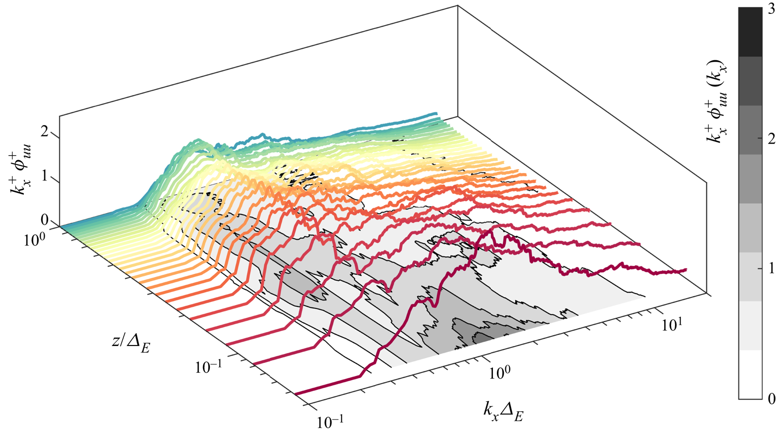
Figure 7. Premultiplied energy spectra of the streamwise velocity obtained from the wind LiDAR measurements.
As mentioned in § 3.2, from the streamwise velocity premultiplied spectra calculated at each height,  $A_1$ is estimated heuristically, while the parameter
  $A(z)$ is obtained by fitting the spectrum with (3.12) over the spectral region (iii). An example of this procedure is reported in figure 8(a) for the premultiplied streamwise velocity spectrum evaluated for the LiDAR data collected at a height of 16 m. A spectral region with roughly constant energy, i.e. corresponding to region (ii
 $_A$), is identified in the proximity of the low-frequency limit of region (i) (
 $k_x\varDelta _E\approx 5$). The fitting of (3.9) for the model of region (i) with the experimental spectrum is reported with a dashed line over the high-frequency part of the spectrum, while the fitting with (3.12) for the model of region (iii) is also reported with a dashed line over the low-frequency part of the spectrum. The intersections between the horizontal dashed line corresponding to the identified value of
  $A_1$ (
 ${\approx }0.91$ for the LiDAR data reported in figure 8a) and the modelled spectra for regions (i) and (iii) enable the identification of the non-dimensional spectral limit
  $P$ (red circle in figure 8a) and
  $F$ (blue triangle in figure 8a), respectively. Finally, for the identification of the spectral limit
  $G$, the part of region (ii) with energy larger than
  $A_1$ yet reducing with increasing wavenumber is considered. The spectral limit
  $G$ is associated with the intersection of this part of the spectrum with the horizontal dashed line corresponding to
  $A_1$.
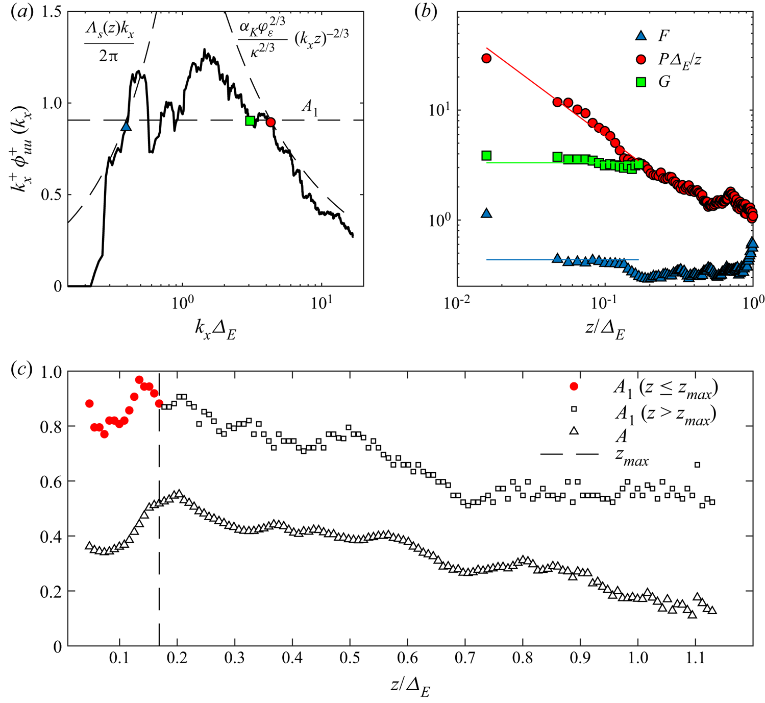
Figure 8. Identification of spectral limits from the streamwise velocity energy spectra. (a) Detection of the spectral limits for the LiDAR velocity signal collected at a 16 m height. (b) Wall-normal profiles of  $F$,
$F$,  $G$ and
  $P$. (c) Vertical profiles of
  $A_1$ (red circles for
  $z\leq z_{max}$ and black squares for
  $z > z_{max}$) and
  $A$.
$A$.
The vertical profiles of the spectral limits  $P$,
$P$,  $G$ and
  $F$ obtained from the analysis of the premultiplied streamwise velocity energy spectra are reported in figure 8(b). First, it is observed that, as predicted from the AEH (see § 1), the non-dimensional spectral limits
  $G$ and
  $F$ are roughly invariant with
  $z$. Specifically,
  $G$ has a mean value of about 3.3, which corresponds to a wavelength of
  $1.9\varDelta _E$, while
  $F$ has a mean value of 0.44, which corresponds to a wavelength of
  $14.3\varDelta _E$. In contrast, the spectral limit between region (i) and region (ii
 $_A$),
  $P$, decreases with the wall-normal position, which confirms its inertial-scaling consistently with the predictions of Perry & Chong (Reference Perry and Chong1982), Perry et al. (Reference Perry, Henbest and Chong1986) and the experimental results of Nickels et al. (Reference Nickels, Marusic, Hafez and Chong2005), Hwang (Reference Hwang2015), Baars et al. (Reference Baars, Hutchins and Marusic2017) and Hu et al. (Reference Hu, Yang and Zheng2020) for laboratory flows. The linear fitting of the profile reported in figure 8(b) produces an estimate for
  $P$ of 0.58, which corresponds to an eddy aspect ratio of
  $\lambda _x/z=2{\rm \pi} /0.58\approx 10.8$, which is smaller than the value of 14 estimated in Baars et al. (Reference Baars, Hutchins and Marusic2017) through the LCS analysis of data sets collected with a wide range of Reynolds number flows, including an ASL case as well.
As mentioned in § 3.2, the intersection between  $P\varDelta _E/z$ and
  $G$ identifies the maximum height where region (ii
 $_A$) is observed, i.e.
  $z_{max}\approx 21$ m (
 $0.17\varDelta _E$). It is noteworthy that this outer-scaled value coincides with that provided by Hwang (Reference Hwang2015) and it is close to the results by Baars & Marusic (Reference Baars and Marusic2020b) (
 $0.15\varDelta _E$), while it is lower than the value proposed by Hu et al. (Reference Hu, Yang and Zheng2020) (
 $0.53\varDelta _E$).
In addition to the limits amongst the different spectral regions, it is important to analyse the vertical profile of the parameter  $A_1$, which is heuristically estimated from the premultiplied spectra of the streamwise velocity. In the perspective of the AEH,
  $A_1$ can be estimated only for wall-normal positions lower than
  $z_{max}$, namely for heights where the spectral region (ii
 $_A$) can be detected. However, in this work, a value is still associated with
  $A_1$ even aloft, which corresponds to the average energy within the spectral range between regions (i) and (iii). The obtained wall-normal profile of
  $A_1$ is reported in figure 8(c), specifically reporting values for heights below
  $z_{max}$ with red circles and aloft with black squares. Starting from the lowest height and moving upwards,
  $A_1$ increases from a value of about 0.8 up to about 1 at
  $z/\varDelta _E\approx 0.13$. While the obtained values are reasonable according to previous works (e.g.
  $A_1=0.80$ for channel flows and
  $A_1=1.0$ for ASL and boundary layers (Hu et al. Reference Hu, Yang and Zheng2020), while
  $A_1=0.975$ for boundary layers Baars & Marusic Reference Baars and Marusic2020b), the variability of
  $A_1$ with height is not in agreement with the AEH predictions. Furthermore, for wall-normal positions above
  $z_{max}$, the mean energy roughly monotonically reduces up to
  $z/\varDelta _E\approx 0.7$, then it remains roughly constant aloft.
An interpretation of these experimental results might be provided by analysing the vertical profile of the parameter  $A(z)$, which represents the energy level over region (iii) as a function of height and it is connected with the vertical variability of the turbulent kinetic energy associated with large-scale turbulent motions. Figure 8(c) shows that
  $A(z)$ increases from 0.37 up to 0.60 between
  $0.1\varDelta _E$ and
  $0.2\varDelta _E$, followed by a roughly monotonic decrease aloft. These values are comparable to those reported by Högström et al. (Reference Högström, Hunt and Smedman2002), namely
  $A(z)$ increases from 0.2 up to 1 at a height of
  $z=0.3\varDelta _E$, then it decreases aloft. The similar trends obtained for
  $A_1$ and
  $A(z)$ as a function of the wall-normal position suggest that even though a roughly flat region of the premultiplied spectra can be singled out over the region (ii
 $_A$), the values attained by
  $A_1$ can significantly be affected by an underlying energy contribution associated with VLSMs, which is a reasonable feature within region (ii) where wall-attached and coherent structures with larger wavelengths co-exist and, thus, their energy contributions overlap.
To better visualize the boundaries of the various spectral regions, the streamwise velocity premultiplied energy spectra are reported in figure 9 with a grey colour map. The estimated spectral limits for the different heights,  $P$,
$P$,  $G$ and
  $F$, are reported as well with red circle, green square and blue triangle markers, respectively. The spectral limits of region (ii) estimated from the above-mentioned previous works are also reported in that figure. For heights below 0.17
 $\varDelta _E$, the wall-normal trend of the spectral limit
  $P$ has a good level of agreement with the findings for channel flows by Hwang (Reference Hwang2015), where the aspect ratio of the wall-attached eddies was estimated as
  ${A{\kern-4pt}R} =12$. The present results for
  $P$ are slightly larger than the spectral limit estimated through the LCS in Baars et al. (Reference Baars, Hutchins and Marusic2017), where the authors estimated
  ${A{\kern-4pt}R} =14$ for boundary layers.
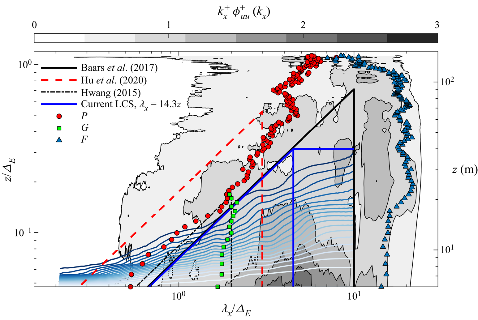
Figure 9. Premultiplied energy spectra of the LiDAR streamwise velocity measurements reported as a grey colour map (isocontour levels from 0.4 up to 3 with a 0.4 step). The LCS are reported as blue-scaled contour lines (isocontour levels from 0.1 up to 1 with a 0.05 step).
From the analysis of the spectral limit  $G$ between regions (ii
 $_A$) and (ii
 $_B$) (green squares in figures 8(b) and 9), the average value of
  $\lambda _x=1.9\varDelta _E$ is close to that obtained by Hwang (Reference Hwang2015) (
 $\lambda _x=2\varDelta _E$). For the spectral limit between regions (ii) and (iii), the outer-scaled wavelength associated to
  $F$ (blue triangles in figures 8(b) and 9) is quantified as
  $14.3\varDelta _E$ below
  $z_{max}$ and
  $15.8\varDelta _E$ above, both within the interval provided by Hutchins et al. (Reference Hutchins, Chauhan, Marusic, Monty and Klewicki2012) for the maximum streamwise extent of VLSMs in a boundary layer, i.e. between 10
 $\varDelta _E$ and 20
 $\varDelta _E$. Finally, the comparison for the spectral limits of region (ii) obtained from the current investigation with those from previous studies (Hwang Reference Hwang2015; Baars et al. Reference Baars, Hutchins and Marusic2017; Hu et al. Reference Hu, Yang and Zheng2020) are summarized in table 2.
Table 2. Identification of the various regions from the energy spectra and LCS of the streamwise velocity. The acronyms TBL, CH and ASL stand for turbulent boundary layer, channel flow and atmospheric surface layer, respectively.
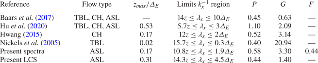
4.2. Detection of different energy contributions in the LiDAR measurements through the LCS
The energy contributions associated with different eddy typologies are further investigated through the analysis of the LCS, which is calculated according to (3.15) through the Welch (Reference Welch1967) algorithm and leveraging as reference the velocity signal collected from the lowest LiDAR gate ( $z_{R}\approx 0.05\varDelta _E$). Specifically, each signal is subdivided into windows with a 179 s duration (corresponding to nearly
  $18 \varDelta _E$ leveraging the Taylor's hypothesis of frozen turbulence Taylor Reference Taylor1938) and
  $90\,\%$ overlapping between consecutive windows to estimate the auto- and cross-spectra of the streamwise velocity. It is noted that the values for the window duration and overlapping of the various data subsets do not distort the LCS at lower frequencies, while these parameters are more important for ensuring a roughly null LCS at higher frequencies. Each LCS is smoothed, as performed for the energy spectra. For more details on the calculation of the LCS and the determination of its parameters see Appendix C. The LCS calculated from the LiDAR measurements is reported as blue isocontours over the (
 $\lambda _x, z$) domain in figure 9.
The parameters of the analytical LCS model for wall-attached eddies (3.21) are quantified by fitting the LCS calculated from the LiDAR measurements. According to the point (b) discussed in § 3.4, for a fixed  $\lambda _x$,
  $\gamma ^2$ is a linear function of
  $\log (z/z_R)$ with a slope equal to
  $-C_1$ for heights above
  $z_R$. To this aim,
  $\lambda _x$ is selected within the interval between
  $3.5\varDelta _E$ and
  $9.5\varDelta _E$ to avoid effects due to small-wavelength eddies and large-wavelength non-turbulent contributions, respectively. The portions of
  $\gamma ^2$ varying roughly linearly with
  $\log (z/z_R)$, which are reported with a red colour scale in figure 10(a), are fitted with a linear function of
  $\log (z/z_R)$ to estimate the intercept
  $I$ and the slope
  $-C_1$, which are then reported in figure 10(b) with square and circle markers, respectively. Here
  $C_1$ has roughly constant values for different
  $\lambda _x$, as predicted from the analytical model for the LCS of (3.22), with an average value of
  $C_1=0.485$.
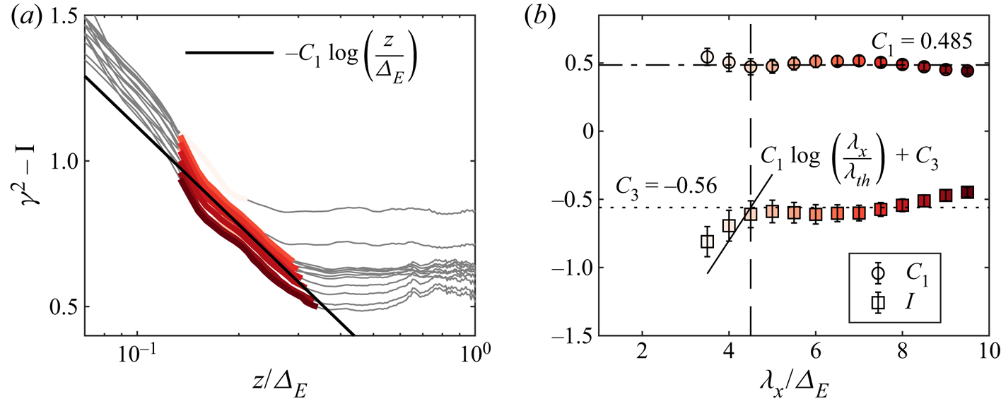
Figure 10. LCS of the LiDAR measurements using  $z_{R}/\varDelta _E\approx 0.05$; (a)
  $\gamma ^2-I$ for fixed values of
  $\lambda _x$; (b) fitted values of
  $C_1$ and
  $I$ from (3.22), the error bars refer to
  $95\,\%$ confidence level. The parameter
  $\lambda _x^{th}$ is reported with a vertical dashed line.
For  $z\geq z_R$, the analytical LCS model predicts that the intercept of
  $\gamma ^2$,
  $I$, should be a linear function of
  $\log (\lambda _x)$ for
  $\lambda _x\leq \lambda _x^{th}$, while achieving an asymptotic value equal to
  $C_3$ for
  $\lambda _x>\lambda _x^{th}$ (3.22). In figure 10(b) the values of
  $I$ confirm these predictions, specifically showing an asymptotic value of the intercept of
  $C_3\approx -0.56$ for
  $\lambda _x/\varDelta _E\geq 4.5$, thereby assumed as
  $\lambda _x^{th}$. An assessment of the results obtained with this fitting procedure is performed considering that the intercept of
  $\gamma ^2$ should vary as
  $C_1\log (\lambda _x/\lambda _x^{th})+C_3$ for
  $\lambda _x\leq \lambda _x^{th}$ and
  $z\geq z_R$. This function, which is reported in figure 10(b) with a black solid line using the fitted values obtained for
  $C_1$ and
  $C_3$, and
  $\lambda _x^{th}$ shows a good agreement with the experimental data considering the small number of samples available for
  $\lambda _x\leq \lambda _x^{th}$.
Recalling that  $\log (\lambda _x^{th}/\varDelta _E)=C_3/C_1+\log ({A{\kern-4pt}R} )$, we can estimate the aspect ratio of the coherent eddies as
  ${A{\kern-4pt}R} \approx 14.3$. Finally, the maximum height attained by wall-attached eddies is estimated from (3.23b), namely
  $z_{max}/\varDelta _E=\exp (C_3/C_1)\approx 0.31$. This estimate of
  $z_{max}$ obtained from the LCS analysis is larger than that obtained from the analysis of the energy spectra, i.e.
  $0.17\varDelta _E$ (§ 4.1), as well as the estimates obtained by Hwang (Reference Hwang2015) and Baars & Marusic (Reference Baars and Marusic2020b) (
 $0.17\varDelta _E$ and
  $0.15\varDelta _E$, respectively); furthermore, the spectral approach of Hu et al. (Reference Hu, Yang and Zheng2020) returns a sensibly larger value of
  $z_{max}$ (
 $0.53\varDelta _E$). Finally, in Baars et al. (Reference Baars, Hutchins and Marusic2017), for an aspect ratio of 14, the authors estimated
  $\lambda _x^{th}=10\varDelta _E$ based on
  $z_{max}=0.71\varDelta _E$.
The estimate of  $z_{max}/\varDelta _E\approx 0.31$ obtained from the LCS analysis agrees with the vertical extent of the ESL for ASL flows, which was previously estimated equal to
  $0.3\varDelta _E$ (Hunt & Morrison Reference Hunt and Morrison2000; Högström et al. Reference Högström, Hunt and Smedman2002; Drobinski et al. Reference Drobinski, Carlotti, Redelsperger, Banta, Masson and Newsom2007). In the existing literature, the ESL is considered as the layer where the vertical confinement induced by the wall affects the dynamics and evolution of eddies entraining the boundary layer from aloft that, in turn, contribute to the generation of new turbulence structures from the wall. Our analysis seems to indicate that the ESL is dominated by a hierarchical distribution of eddies statistically attached to the wall.
The calibrated LCS model, and specifically the  $\gamma ^2=0$ condition (3.23a), is now compared with the experimental values of
  $\gamma ^2$, as reported in the colour map of figure 9. Analysing the darkest isocontour with
  $\gamma ^2=0.1$, a deviation from the predicted unitary slope of the LCS isocontours is observed for
  $z\lessapprox 0.12\varDelta _E$, which is due to the local contribution of small, wall-incoherent structures (type-
 $\mathcal {C}$ eddies) (Krug et al. Reference Krug, Baars, Hutchins and Marusic2019; Baars & Marusic Reference Baars and Marusic2020a) as a consequence of the small vertical separation between
  $z_R$ and the wall-normal position of these LiDAR data. Moving towards higher vertical positions and for
  $\lambda _x/\varDelta _E\approx 2$, a unitary slope of the isocontours is recovered, in agreement with the LCS model (3.23a), and in agreement with previous experimental results (Baars et al. Reference Baars, Hutchins and Marusic2017; Baars & Marusic Reference Baars and Marusic2020a; Li et al. Reference Li, Wang and Zheng2021). For higher wall-normal positions, a further deviation from the model prediction is observed, which may be ascribed to a residual thermal stratification still present in the ASL flow considering the early morning time of the data collection (local time between 3:00 AM and 4:00 AM), as already observed from previous field experiments (Krug et al. Reference Krug, Baars, Hutchins and Marusic2019).
It is noteworthy that the zero-LCS contour predicted with (3.23a) has a relatively good agreement with the vertical profile of the spectral limit  $P$ between regions (i) and (ii
 $_A$) identified through the analysis of the streamwise velocity energy spectra in § 4.1 (figure 9), yet translated towards slightly larger wavelengths. An aspect ratio of 14.3 is estimated indeed from the LCS analysis, while
  ${A{\kern-4pt}R} \approx 10.8$ from the analysis of the energy spectra. Nonetheless, this result can be considered as proof that the inverse-power-law region of the streamwise velocity energy spectra is associated with wall-attached eddies (Perry et al. Reference Perry, Henbest and Chong1986), and the LCS approach resonates with the spectral approach to identify the
  $k_x^{-1}$ high-frequency limit.
The LCS analytical model calibrated through the LiDAR data for the high-frequency limit (3.23a) is in good agreement with the analysis based on the LCS presented in Baars et al. (Reference Baars, Hutchins and Marusic2017) for boundary layers ( ${A{\kern-4pt}R} =14$), while a slightly smaller aspect ratio (
 ${A{\kern-4pt}R} =12$) was estimated in Hwang (Reference Hwang2015) for channel flows. In contrast, the high-frequency spectral limit provided in Hu et al. (Reference Hu, Yang and Zheng2020) with
  ${A{\kern-4pt}R} =5.7$ seems to be an underestimate for the present data set.
Regarding the spectral boundary between the energy associated with wall-attached eddies and that due to larger coherent structures, the spectral limit  $G$ estimated through the analysis of the streamwise velocity energy spectra is about 1.9
 $\varDelta _E$, which is very similar to the respective limit estimated by Hwang (Reference Hwang2015), and is significantly lower than the value of 4.5
 $\varDelta _E$ obtained from the present LCS analysis through
  $\lambda _x^{th}$. For the sake of completeness,
  $G$ was estimated equal to 2.09
 $\varDelta _E$ in Hu et al. (Reference Hu, Yang and Zheng2020) and 10
 $\varDelta _E$ in Baars et al. (Reference Baars, Hutchins and Marusic2017) (estimated indirectly from
  ${A{\kern-4pt}R}$ and
  $z_{max}$). This analysis would suggest that the analysis of streamwise velocity energy spectra should lead to an underestimate of the spectral limit
  $G$ due to the co-existence of energy contributions associated with eddies of different typologies. In contrast, the present LCS approach should offer a more reliable approach to separate wall-attached spectral energy from that associated with larger coherent structures.
Finally, the present LCS method does not provide a criterion to identify the low-frequency limit of the spectral region (ii $_B$),
  $F$, which is then only identifiable through the analysis of the streamwise velocity energy spectra.
4.3. LCS calculated with increasing reference height
Once the LCS analysis is performed with the reference height  $z_R=0.05\varDelta _E$, a similar analysis is carried out by increasing
  $z_R$, which can provide more insights into the LCS analytical model (3.21), especially for
  $z< z_R$. However, we do not expect this analysis to further contribute to the foregoing discussion for
  $z>z_R$ because, with increasing
  $z_R$, the vertical range where incremental contributions associated with wall-attached eddies can be observed,
  $z_{max}-z_R$, reduces. To this aim, six additional reference heights are selected, namely
  $0.20\varDelta _E,\ 0.25\varDelta _E,\ 0.30\varDelta _E, 0.45\varDelta _E,\ 0.50\varDelta _E$ and
  $0.70\varDelta _E$.
The LCS maps obtained for all the considered  $z_R$ values are reported as isocontours in figure 11; further, the
  $\gamma ^2=0$ isocontours estimated analytically through (3.23) are also reported using the parameters
  $C_1$,
  $C_3$ and
  ${A{\kern-4pt}R}$ calibrated as for § 4.2. For the region at smaller wavelengths demarcated by the analytically predicted
  $\gamma ^2=0$ isocontours, it is evident that the experimental LCS obtained from the LiDAR measurements do not follow the analytical model of (3.21), rather they are dominated by energy contributions associated with wall-detached type-
 $\mathcal {C}$ eddies (Krug et al. Reference Krug, Baars, Hutchins and Marusic2019; Baars & Marusic Reference Baars and Marusic2020a). However, with increasing
  $z_R$, thus increasing the vertical distance between
  $z_R$ and the lower LiDAR sampling heights, which is advantageous to reduce the effects of type-
 $\mathcal {C}$ eddies on the LCS, a roughly vertical
  $\gamma ^2=0$ isocontour is observed already for
  $z_R/\varDelta _E=0.2$, which is even more evident for
  $z_R/\varDelta _E=0.25$ and
  $0.3$. As predicted through the LCS analytical model (3.23c), for
  $z< z_R$, the
  $\gamma ^2=0$ isocontour should occur for
  $\lambda _x={{A{\kern-4pt}R} }z_R$, which is indeed in good agreement for all the
  $z_R$ values used for this analysis below
  $z_{max}$ by assuming
  ${A{\kern-4pt}R} =14.3$ as estimated in § 4.2. The vertical
  $\gamma ^2=0$ isocontour becomes less evident with increasing
  $z_R$, until it disappears completely for
  $z_R/\varDelta _E=0.7\varDelta _E$, indicating that no structures originating from below
  $z_R=0.7$ are coherent with that reference position.
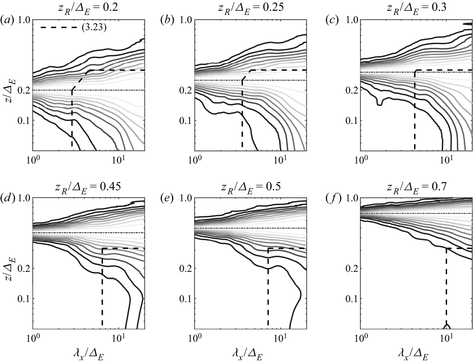
Figure 11. Isocontours (values from 0.1 up to 1 with a step of 0.1) of the LCS obtained with different  $z_R$ (horizontal dot-dashed lines). The
  $\gamma ^2=0$ contours predicted through the model in (3.23) are reported with a dashed line.
The maps of the streamwise velocity energy spectra for the coherent (figure 12) and incoherent (figure 13) components calculated for all the selected reference heights are now analysed. Starting from the lowest reference height,  $z_R=0.05\varDelta _E$, it is observed that the coherent energy is practically confined within the
  $\gamma ^2=0$ limit predicted in (3.23a) and the maximum height (3.23b) (figure 12a). The energy peak is observed at the lowest height (
 $z_R=0.05\varDelta _E$) at a wavelength
  $\lambda _x/\varDelta _E\approx 5.2$. This is practically the upper region of the outer energy peak already observed by, e.g. Wang & Zheng (Reference Wang and Zheng2016) for atmospheric flows.
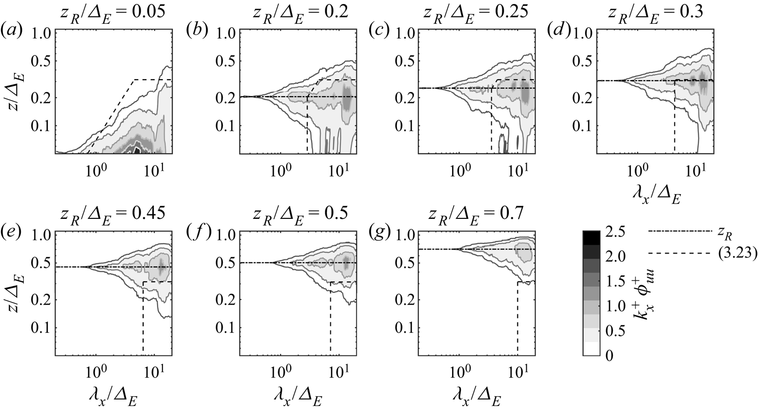
Figure 12. Coherent portion of the streamwise velocity energy spectra calculated for different reference heights,  $z_R$.
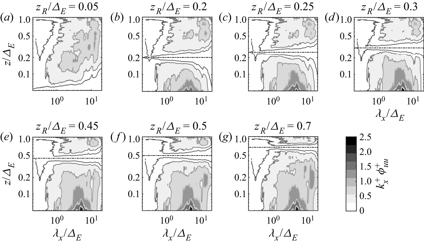
Figure 13. Incoherent portion of the streamwise velocity energy spectra calculated for different reference heights,  $z_R$.
On the other hand, figure 13(a) shows that the incoherent component obtained using  $z_R=0.05\varDelta _E$ encompasses energy across the entire spectral range considered and up to
  $\varDelta _E$. Furthermore, the energy seems to move towards larger wavelengths with increasing height, which is a similar feature predicted from the AEH for wall-attached eddies. This suggests that also wall-detached eddies might be affected by the wall confinement of the flow and the local shear in the boundary layer. The incoherent energy component may be thought of as the footprint of shear surface layer structures entraining from above via top–down motions (Hunt & Morrison Reference Hunt and Morrison2000; Högström et al. Reference Högström, Hunt and Smedman2002; Morrison Reference Morrison2007); thus, incoherent with a reference height located in the ESL.
With increasing reference height, i.e. for  $z_R=0.2\varDelta _E$, the coherent energy below
  $z_R$ (figure 12b) drastically reduces compared with the case with
  $z_R=0.05\varDelta _E$ (figure 12a), and the remaining coherent energy is mainly located towards large wavelengths (
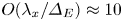 $O(\lambda _x/\varDelta _E)\approx 10$). This indicates that a cluster of coherent structures originated below
  $z_R=0.2\varDelta _E$, i.e. wall-attached eddies, does not attain this height, and only taller wall-attached eddies are left in the coherent energy component, which are characterized by larger wavelengths indeed.
For the same reason, increasing the reference height from  $0.05\varDelta _E$ to
  $0.2\varDelta _E$ leads to enhanced incoherent energy below
  $z_R$ (compare figure 13(b) with 13(a)). This added energy resembles the coherent energy obtained with
  $z_R=0.05\varDelta _E$ (figure 12a). Therefore, this analysis corroborates that the increase of reference height from
  $0.05\varDelta _E$ to
  $0.2\varDelta _E$ mainly leads to transferring a certain energy packet associated with wall-attached eddies from the coherent to the incoherent component.
It is noteworthy that in figure 12(b) a significant amount of coherent energy is singled out around  $z_R=0.2\varDelta _E$, which is the effect on the LCS due to type-
 $\mathcal {C}$ eddies and their streamwise concatenation. A similar feature is observed for all the reference heights located above
  $0.05\varDelta _E$ (figure 12b–g).
A similar trend is observed with increasing  $z_R$ below
  $z_{max}\approx 0.31 \varDelta _E$, i.e. reduced coherent energy and increased incoherent energy below
  $z_R$, while above
  $z_{max}$, i.e. in figure 12(e–g), the coherent component shows only the contribution associated with type-
 $\mathcal {C}$ eddies and no energy extending below, indicating no contribution due to wall-attached eddies. On the other hand, above
  $z_{max}$, the incoherent component achieves practically an asymptotic energy map for
  $z< z_{max}$, and only energy at large scales for
  $z>z_{max}$ are added with increasing
  $z_R$, which confirms that no wall-attached eddies are statistically present above
  $z_{max}$.
4.4. Streamwise turbulence intensity
The energy contributions to the streamwise velocity associated with wall-attached eddies and larger coherent structures have been identified through the analysis of the streamwise velocity energy spectra (§ 4.1), and the LCS (§ 4.2). Considering that the streamwise turbulence intensity is the integrated spectral energy across scales, it is then possible to distinguish the contributions to  $\overline {uu}$ associated with eddies of different typologies. The streamwise turbulence intensity obtained using the integration limits estimated either from the spectral analysis (§ 4.1) or the LCS (§ 4.2) are reported in figure 14(a) with black and blue markers, respectively. Specifically, the streamwise turbulence intensity associated with wall-attached eddies,
  $\overline {uu}_{ii,A}$, is obtained by integrating the streamwise velocity energy spectra between the limits
  $P$ and
  $G$ for the spectral method, while for the LCS method, the integration is performed between the limits
  $\lambda _x={{A{\kern-4pt}R} }z$ and
  $\min [\lambda _x={{A{\kern-4pt}R} }z\exp {1/C_1}, \lambda _x^{th}]$ (3.23) and (3.24). Similarly,
  $\overline {uu}_{ii,B}$ is obtained by integrating the energy spectra between the limits
  $G$ and
  $F$ for the spectral method, and between
  $\min [\lambda _x={{A{\kern-4pt}R} }z \exp {1/C_1}, \lambda _x^{th}]$ and
  $\lambda _x/\varDelta _E=2{\rm \pi} /F$, namely using the same low-frequency limit estimated through the spectral method.
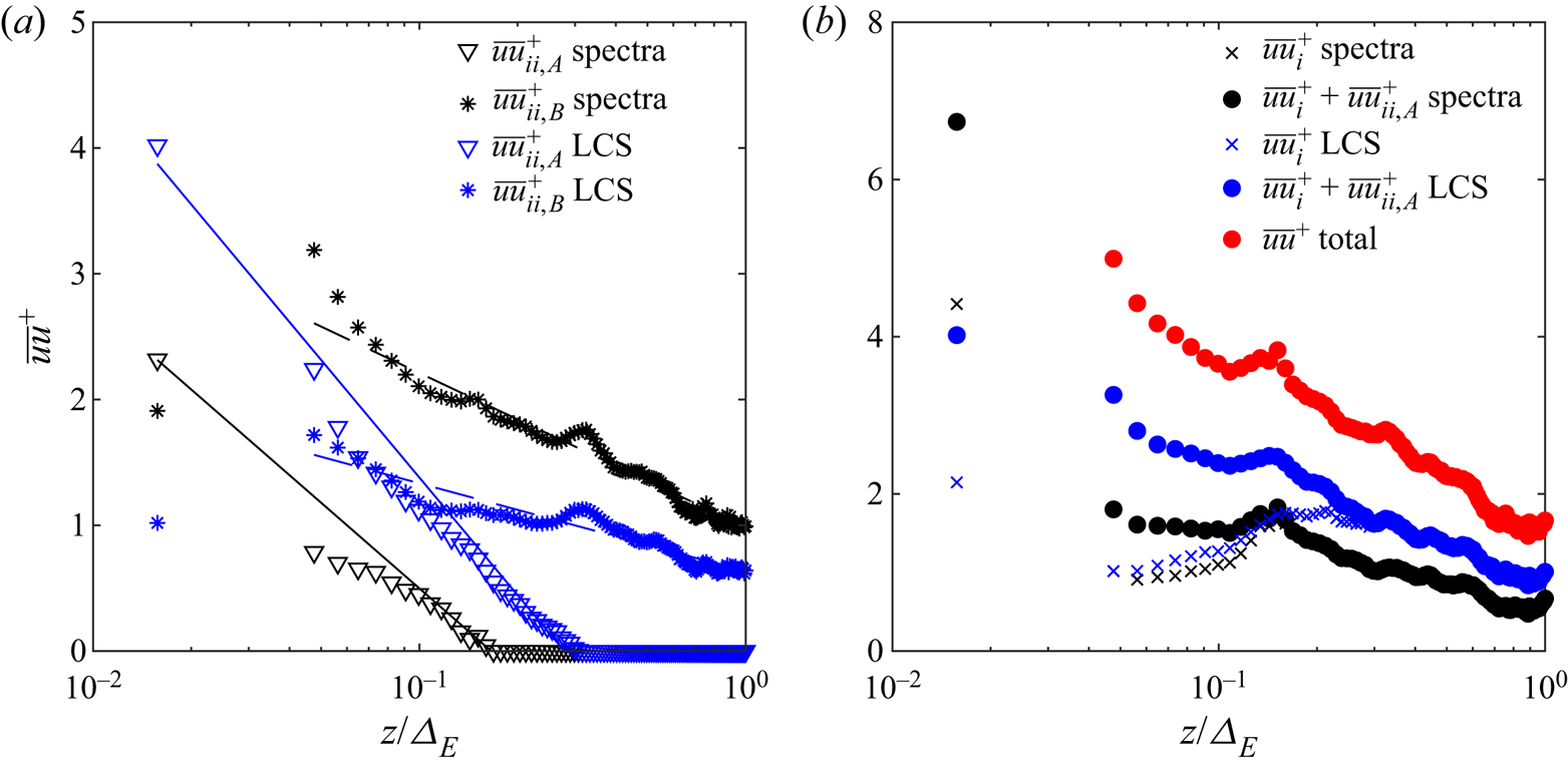
Figure 14. Vertical profiles of the streamwise turbulence intensity considering different eddy typologies and identification techniques. (a) Contributions over region (ii $_A$) and (ii
 $_B$) identified through the spectral method and the LCS. (b) Cumulative contributions to
  $\overline {uu}$.
Concerning the model for  $\overline {uu}_{ii,A}^+$ derived from the AEH (2.9), in figure 14(a) the data seemingly shows a logarithmic vertical profile for both spectral and LCS methods, even though with significant differences in energy content and maximum height. The wall-attached component
  $\overline {uu}_{ii,A}$ is lower for the spectral method than for the LCS method, because, as reported in § 4.1, while the spectral limit
  $P$ is slightly larger for the spectral method, the spectral limit
  $G$ is significantly overestimated with respect to the LCS outcome (shorter spectral range between
  $P$ and
  $G$ for the spectral method), due to the overlap of the energy associated with larger coherent structures, e.g. VLSMs and superstructures, concealing the flat part of the premultiplied streamwise velocity energy spectra of region (ii
 $_A$). For the same reason, the component
  $\overline {uu}_{ii,B}$ is larger for the spectral method than for the LCS method. Similarly,
  $z_{max}$ estimated from the spectral analysis is lower than that obtained from the LCS analysis being the limit
  $2{\rm \pi} /G$ smaller than
  $\lambda _x^{th}\approx 4.5$ estimated through the LCS method, thus the intersection of the high-frequency limit of the spectral region (ii
 $_A$) with the low-frequency limit occurs at higher wall-normal positions for the results obtained from the LCS.
The vertical profiles of  $\overline {uu}^+_{ii,A}$ are fitted with the model based on the AEH in (2.9) to estimate the parameters
  $A_1$ and
  $B_1$, which are reported in table 3. It is noteworthy that the fitting has been limited to LiDAR gates with
  $z\geq 18$ m, which is the LiDAR range gate, to avoid possible underestimation of
  $\overline {uu}$ due to the LiDAR spatial averaging over the probe volume (see Appendix B). As shown in table 3,
  $A_1$ is generally estimated very close to 1, namely equal to 0.98 or 1.35 if estimated through the spectral or the LCS method, respectively. The former is very close to the recent estimate provided by Baars & Marusic (Reference Baars and Marusic2020b) (0.975) where only the wall-attached-eddy contribution is considered. Thus, the spectral method seems to return the correct energy rate with height for the wall-attached-eddy component to the turbulence intensity, even though
  $\overline {uu}_{ii,A}$ can be underestimated. The values for
  $B_1$ are very close, namely
  $-$1.76 and
  $-$1.73 for the spectral and the LCS method, respectively. In Baars & Marusic (Reference Baars and Marusic2020b),
  $B_1$ for
  $\overline {uu}_{ii,A}^+$ was estimated equal to
  $-$2.26.
Table 3. Values of  $A_1$ and
  $B_1$ of (2.9) calibrated with different methods and spectral regions. Uncertainty intervals refer to a
  $95\,\%$ confidence level.
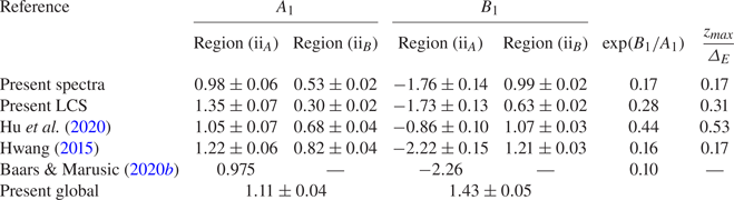
The best fit of the experimental profiles of  $\overline {uu}^+_{ii,A}$ with (2.9) is also performed for the vertical profiles obtained using the spectral limits proposed by Hwang (Reference Hwang2015) and Hu et al. (Reference Hu, Yang and Zheng2020), whose results are reported in table 3. The spectral boundaries of Hu et al. (Reference Hu, Yang and Zheng2020) lead to a fitted value of
  $A_1$ comparable with that estimated by the authors (
 $0.98$ vs 1.0) while using the spectral limits proposed by Hwang (Reference Hwang2015) leads to an estimate closer to the value obtained with the LCS method, i.e.
  $A_1=1.22$.
From (2.9), we can estimate the height where  $\overline {uu}_{ii,A}^+$ becomes zero, i.e.
  $z_{max}/\varDelta _E=\exp (B_1/A_1)$, which is reported in table 3 and compared against the previously reported values of
  $z_{max}$ estimated independently from the streamwise velocity energy spectra or the LCS. A good agreement between
  $z_{max}/\varDelta _E$ and
  $\exp (B_1/A_1)$ is generally observed for the different methods used for the detection of the energy contribution associated with wall-attached eddies, meaning that the selected streamwise energy is mainly limited to wall-attached-eddy contributions.
Focusing on the energy associated with large coherent structures (star markers in figure 14a), a logarithmic wall-normal trend of  $\overline {uu}_{ii,B}^+$ is seemingly observed throughout the vertical range probed by the LiDAR, as already noted in Hu et al. (Reference Hu, Yang and Zheng2020), for both spectral and LCS methods. The results for
  $B_1$ and
  $A_1$ obtained by fitting
  $\overline {uu}^+_{ii,B}$ with (2.9) are reported in table 3 for all the considered spectral boundaries. First,
  $A_1$ for the wall-detached component is significantly smaller than for the wall-attached counterpart, specifically
  $A_1$ equal to 0.53 and 0.3 for the spectral and LCS methods, respectively. The parameter
  $B_1$ is positive, while for
  $\overline {uu}^+_{ii,A}$, it is generally negative and close to one.
It is noteworthy that the value of  $\overline {uu}^+_{ii,B}$ measured by the sonic anemometer at
  $z/\varDelta _E=0.025$ is smaller than the maximum value of
  $\overline {uu}^+_{ii,B}$ measured by the LiDAR at
  $z/\varDelta _E=0.05$. This result is consistent with the work by Hu et al. (Reference Hu, Yang and Zheng2020), where a maximum of
  $\overline {uu}^+_{ii,B}$ was observed at
  $z/\varDelta _E=0.045$. Unfortunately, more data between the minimum height probed by the LiDAR (
 ${\approx }6$ m) and the 2 m height of the sonic anemometer would be needed to draw more firm conclusions on the lower part of the vertical profile for
  $\overline {uu}_{ii,B}^+$.
Finally, a cumulative analysis of the streamwise turbulence intensity is reported in figure 14(b) for both spectral and LCS methods. The streamwise turbulence intensity associated with type- $\mathcal {C}$ eddies (
 $\overline {uu}^+_i$ with cross-symbols) is added to the energy associated with wall-attached eddies (blue and black circles), then the total streamwise turbulence intensity is achieved by adding the components associated with VLSMs.
5. Concluding remarks
A study of a high-Reynolds-number near-neutral ASL flow has been presented. The streamwise velocity was measured with a scanning Doppler pulsed wind LiDAR from a height of 6 m up to 143 m with a vertical resolution of approximately 1.08 m, and a sonic anemometer deployed at a 2 m height. The main goal of this study is to identify the energy contributions in the streamwise velocity associated with wall-attached eddies and larger coherent structures. Furthermore, the maximum height attained by wall-attached eddies has been estimated as well.
After quality control of the LiDAR data, assessment of their statistical stationarity and convergence, quantification of the spectral-gap frequency to filter out non-turbulent motions, i.e. mesoscales, and estimation of the outer scale of turbulence,  $\varDelta _E$, the experimental data have mainly been interrogated through two different approaches: the analysis of the energy spectra and the LCS of the streamwise velocity. The main findings of the present study are summarized as follows.
(i) Based on previous works about the LCS of the streamwise velocity induced by wall-attached eddies in turbulent boundary layers (e.g. Baars et al. Reference Baars, Hutchins and Marusic2017; Krug et al. Reference Krug, Baars, Hutchins and Marusic2019; Baars & Marusic Reference Baars and Marusic2020a) and the present results, an analytical model for the LCS inspired by the AEH (Townsend Reference Townsend1976) has been proposed. This model applies for wall-normal positions both below and above the considered reference height and for both wall-attached eddies and larger coherent structures. The model encompasses three parameters, i.e. the streamwise wavelength divided by the height for wall-attached eddies, i.e. their aspect ratio
${A{\kern-4pt}R}$, a parameter $C_1$, which represents the isolated-eddy contribution to the LCS for a given eddy population density, and an offset $C_3$. The parameter ${A{\kern-4pt}R}$, which is estimated to be about 14.3 from the present LiDAR data set, determines the small-wavelength boundary as a function of height of the spectral energy where contributions due to wall-attached eddies begin to build up, i.e. the spectral boundary between regions (i) and (ii$_A$). The parameter $C_1$ determines the spectral range over which these wall-attached-eddy contributions can be observed, i.e. $\log ({\rm \Delta} \lambda _x/\varDelta _E)=1/C_1$, while the maximum height attained by wall-attached eddies is $\log (z_{max}/\varDelta _E)=C_3/C_1$. It is noteworthy that the estimate of $z_{max}$ from the LCS is analogous to that obtained from the AEH through the vertical law of the streamwise turbulence intensity, i.e. $\log (z_{max}/\varDelta _E)=B_1/A_1$, where $A_1$ is the Townsend–Perry constant. For the LiDAR data set under investigation, it is found that $C_1\approx 0.485$ and $C_3\approx -0.56$, which leads to a maximum height for non-null streamwise turbulence intensity associated with wall-attached eddies of $z_{max}/\varDelta _E\approx 0.31$. Finally, the proposed analytical LCS model enables the estimate of the spectral boundary, $\lambda _x^{th}$, between the energy associated with wall-attached eddies and that due to larger structures generated by their streamwise concatenation. For the present LiDAR data set, it is found that $\lambda _x^{th}/\varDelta _E\approx 4.5$.(ii) The analysis of the streamwise velocity energy spectra has enabled us to identify the
$k_x^{-1}$ region, allegedly associated with wall-attached eddies, for heights below ${\approx }0.17 \varDelta _E$, which is a smaller estimate than that obtained from the LCS analysis ($0.31\varDelta _E$). The high-wavenumber limit, $P$, is found to follow an inertial scaling, i.e. with an increasing wavenumber with increasing wall-normal position according to an aspect ratio of 10.8, which is smaller than the respective estimate from the LCS analysis (${A{\kern-4pt}R} \approx 14.3$). In summary, the analysis of the streamwise velocity energy spectra for the detection of the spectral regions associated with different eddy typologies seems reasonable, although encompassing a high level of uncertainty in the estimates of the actual spectral limits of the various regions and the maximum height attained by wall-attached eddies. The main sources of this uncertainty are the empirical nature of the procedure and the presence of the energy associated with larger coherent structures, such as VLSMs and superstructures, obscuring the part of the premultiplied energy spectra with a roughly constant energy level. Nonetheless, even though the spectral range associated with wall-attached energy and, thus, the respective turbulence intensity are underestimated, the analysis of the streamwise velocity energy spectra enables good estimates of the Townsend–Perry constant.(iii) The streamwise turbulence intensity associated with wall-attached eddies,
$\overline {uu}_{ii,A}$, has been assessed against the AEH prediction. The parameter $A_1$ fitted from $\overline {uu}_{ii,A}^+$ leads to estimates of 0.98 and 1.35 for the spectral and LCS methods, respectively, which are in good agreement with the recent results presented in Baars & Marusic (Reference Baars and Marusic2020b), thus confirming the scaling argument of Perry et al. (Reference Perry, Henbest and Chong1986) for ASL flows. The scattering in the estimates of $A_1$ might be caused by the different spectral limits between regions (ii$_A$) and (ii$_B$) identified with the spectral and LSC approach, which, in turn, leads to different values of integrated energy and, thus, wall-normal distributions. On one hand, the spectral-based underestimation of this boundary ($\lambda _x=1.9\varDelta _E$) leads to a downshift of the wall-normal profile of $\overline {uu}^+_{ii,A}$, yet it returns a more reliable estimate of $A_1$ (0.98) as it encompasses mainly type-$\mathcal {A}$ eddy contributions. On the other hand, the LCS-based estimate of this spectral boundary ($\lambda _x=4.5\varDelta _E$) leads to a cross-influence of larger coherent structures onto the wall-normal profile of $\overline {uu}^+_{ii,A}$, and, thus, to an overestimate of $A_1$. For region (ii$_B$), a logarithmic decay of integrated energy is observed, which seemingly confirms the scenario hypothesized by Hu et al. (Reference Hu, Yang and Zheng2020) of a geometrically similar distribution of VLSMs.


In summary, this work has provided evidence that investigations of a near-neutral ASL flow with a scanning Doppler pulse wind LiDAR can open up research opportunities to investigate high-Reynolds-number turbulent boundary layers, upon the optimal design of the LiDAR scanning strategy and post-processing of the generated observations. In this work, the use of the LCS has enabled the identification of the energy components either coherent or incoherent with the ground, their spectral limits with height and the maximum height attained by wall-attached eddies. However, this current LCS approach shows symptoms of cross-contamination on the wall-attached energy contribution with those generated by type- $\mathcal {C}$ and type-
 $\mathcal {B}$ eddies, which might affect, for instance, the estimate of the Townsend–Perry constant. Finally, other data-driven approaches, coupled with the methods tested for this work, might provide more detailed and accurate analyses of the organization and dynamics of coherent structures in turbulent boundary layers, which might be the focus of future investigations.
Funding
This research has been funded by the National Science Foundation, Fluid Dynamics Program, award no. 1705837, and the NSF CAREER program, award no. 2046160, Program Manager Ron Joslin.
Declaration of interests
The authors report no conflict of interest.
Appendix A. Evaluation of the spectral gap and outer scale of turbulence
A challenge to investigating atmospheric turbulent flows is represented by the coexistence of turbulent scales of motion and background large-wavelength flow fluctuations affecting the entire boundary layer height, which are associated with the mesoscale flow component (e.g. Draxl et al. Reference Draxl, Allaerts, Quon and Churchfield2021). Although the non-turbulent mesoscale velocity fluctuations are expected to occur with larger wavelengths than those associated with turbulence, a systematic method for mesoscale-turbulence separation is still elusive (Högström et al. Reference Högström, Hunt and Smedman2002; Metzger et al. Reference Metzger, Mckeon and Holmes2007). The streamwise velocity energy spectrum typically presents a local minimum at the interface between turbulence and mesoscales, which is referred to as the ‘spectral gap’ (Van der Hoven Reference Van der Hoven1957; Panofsky Reference Panofsky1969; Högström et al. Reference Högström, Hunt and Smedman2002; Wyngaard Reference Wyngaard2004; Metzger et al. Reference Metzger, Mckeon and Holmes2007; Guala et al. Reference Guala, Metzger and McKeon2011; Larsén et al. Reference Larsén, Vincent and Larsen2013, Reference Larsén, Larsen and Petersen2016), while the co-spectrum of the turbulent momentum flux,  $\overline {uw}$, becomes negligible for frequencies lower than the spectral-gap frequency (Metzger et al. Reference Metzger, Mckeon and Holmes2007).
For this work, the premultiplied streamwise velocity energy spectra obtained from the wind LiDAR measurements, and the co-spectrum of the vertical turbulent momentum flux measured from the sonic anemometer ‘PA2’ (figure 1a) are analysed. The energy spectra reported in figure 15(a) versus frequency,  $f$, are calculated at each height sampled with the LiDAR through the Welch spectrogram (Welch Reference Welch1967) using a window length of
  $0.0003$ Hz and
  $10\,\%$ overlapping between consecutive sub-periods. The energy spectra are evaluated over 100 frequencies logarithmically spaced between 10
 $^{-4}$ and 0.5 Hz (the Nyquist frequency), which are then smoothed through a moving-average algorithm with a spectral stencil of
  $f_i\pm 0.35f_i$ for a generic frequency
  $f_i$ (Baars & Marusic Reference Baars and Marusic2020a). The wall-normal average between all the spectra is then calculated and reported in figure 15(a) with a red line. The premultiplied energy spectra of the streamwise velocity indicate the spectral gap at a frequency of about
  $0.0055$ Hz (i.e. period of 181.8 s), which is very close to the value reported in Metzger et al. (Reference Metzger, Mckeon and Holmes2007) (
 $0.005$ Hz) for a neutrally stratified flow probed at the SLTEST facility through a vertical array of sonic anemometers, and it is in good agreement with the detrending period of 198 s (corresponding to
  $0.00505$ Hz) and 180 s (corresponding to
  $0.0055$ Hz) used in Guala et al. (Reference Guala, Metzger and McKeon2011) and Hutchins et al. (Reference Hutchins, Chauhan, Marusic, Monty and Klewicki2012), respectively, to remove mesoscale contributions from the velocity turbulence statistics.
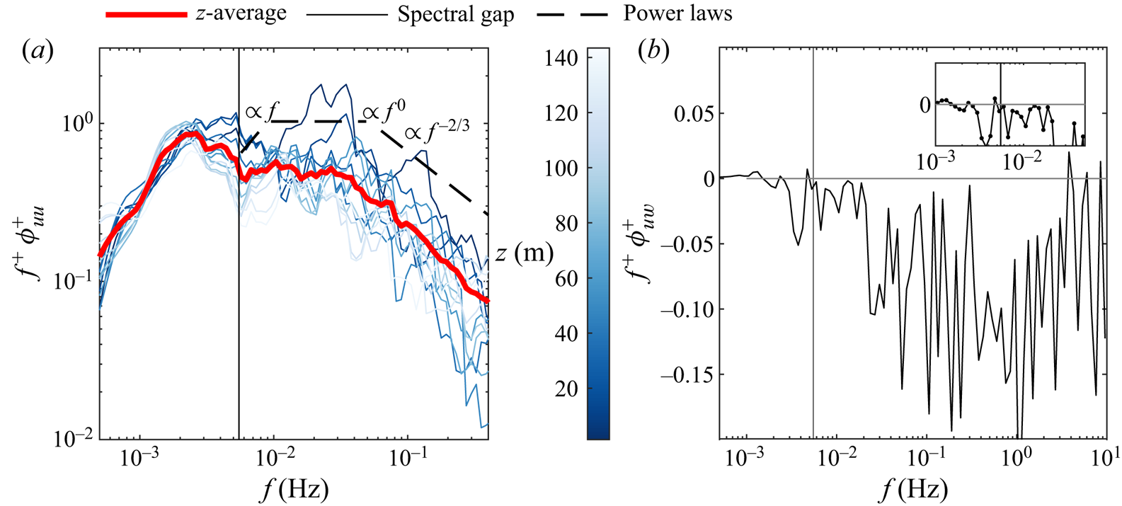
Figure 15. Detection of the spectral gap. (a) Premultiplied streamwise velocity energy spectra of the LiDAR data (the vertically averaged energy spectrum is reported with a red line). (b) Co-spectrum of the vertical turbulent momentum flux measured from the ‘PA2’ sonic anemometer.
The estimate for the spectral-gap frequency is also supported by the analysis of the co-spectrum of the vertical momentum flux measured through the PA2 sonic anemometer (figure 15b), which is obtained through the Welch spectrogram algorithm for 500 frequencies logarithmically spaced between  $10^{-4}$ and 10 Hz (Nyquist value), and using a window length of
  $0.0003$ Hz with a
  $10\,\%$ overlapping period. The co-spectrum is bin averaged over 100 non-overlapping bins to highlight the zero-crossing region at low frequencies, which is approximately located at
  $0.0055$ Hz. The latter is practically equal to the spectral-gap frequency quantified through the LiDAR data.
The quantification of the spectral-gap frequency is also instrumental for the estimate of the outer scale of turbulence,  $\varDelta _E$, which is assumed as the wall-normal position where the turbulence intensity achieves a minimum value (Gryning et al. Reference Gryning, Batchvarova, Floors, Peña, Brümmer, Hahmann and Mikkelsen2014, Reference Gryning, Floors, Peña, Batchvarova and Brümmer2016). For each height, the Weibull probability density function of the streamwise velocity is generated (Gryning et al. Reference Gryning, Floors, Peña, Batchvarova and Brümmer2016),
 \begin{equation} f_u(u) = \frac{S}{B}\left(\frac{u}{B}\right)^{S-1} \exp\left[-\left(\frac{u}{B} \right)^S\right], \end{equation}
where  $S$ and
  $B$ represent the shape and scale parameters, respectively, and
  $u$ is the zero-mean velocity fluctuation. The minimum of the turbulence intensity is identified from the maximum of the shape parameter,
  $S$, throughout the vertical range probed by the LiDAR (Gryning et al. Reference Gryning, Floors, Peña, Batchvarova and Brümmer2016). Subsequently, the vertical profile of
  $S$ is parametrized through the model proposed by Gryning et al. (Reference Gryning, Batchvarova, Floors, Peña, Brümmer, Hahmann and Mikkelsen2014, Reference Gryning, Floors, Peña, Batchvarova and Brümmer2016) for heights lower than
  $\varDelta _E$,
 \begin{equation} S(z;\varDelta_E,c) = S_{min} + c\frac{z-z_{min}}{\varDelta_E-z_{min}} \exp\left(-\frac{z-z_{min}}{\varDelta_E-z_{min}} \right), \end{equation}
where  $S_{min}$ is the shape parameter associated with the lowest height probed,
  $z_{min}$, which is equal to 6 m for the data set under investigation. It should be noted that in Gryning et al. (Reference Gryning, Batchvarova, Floors, Peña, Brümmer, Hahmann and Mikkelsen2014) a second term is added to (A2), which refers to the shape parameter distribution above
  $\varDelta _E$. The outer scale of turbulence and the dimensionless parameter
  $c$ of (A2) are obtained from the least-squares fitting of the vertical profile of
  $S$ estimated from the LiDAR data. It is obtained that
  $\varDelta _E=127\ \textrm {m}\pm 6$ m with a 95 % confidence level, as visualized in figure 16.
Figure 16. Vertical profile of the Weibull shape parameter,  $S$, estimated from the LiDAR velocity signals (black line) and fitted through the model of (A2) (red line).
Appendix B. Spectral correction of the LiDAR velocity measurements
Wind velocity measurements performed with a Doppler wind LiDAR entail an averaging process over each measurement volume, which is mainly affected by the probe length,  $l$, of each laser pulse, and the spatial distribution of the energy within the laser pulse. The radial velocity recorded at a radial distance
  $r$ can be modelled as the convolution between the true radial speed
  $\tilde {V}_r(r,t)$, namely the wind velocity component along the direction of the LiDAR laser beam, and a weighting function
  $\omega (r)$ representing the energy distribution along the laser pulse (Frehlich et al. Reference Frehlich, Hannon and Henderson1998; Frehlich & Cornman Reference Frehlich and Cornman2002; Mann et al. Reference Mann, Cariou, Courtney, Parmentier, Mikkelsen, Wagner, Lindelöw, Sjöholm and Enevoldsen2009; Cheynet et al. Reference Cheynet, Jakobsen, Snæbjörnsson, Mann, Courtney, Lea and Svardal2017; Puccioni & Iungo Reference Puccioni and Iungo2021),
 \begin{equation} V_r(r,t) = \int_{{-}l/2}^{l/2}\tilde{V}_r(r+x',t)\omega(x')\,\text{d}x'. \end{equation}
For the LiDAR unit used for this experiment,  $l=18$ m and
  $\omega =0$ outside of the range gate. The convolution in the physical domain corresponds to a product in the spectral domain between the true streamwise velocity spectrum (
 $\tilde {\phi }_{uu}(k_x)$) and the squared modulus of the Fourier transform of
  $\omega$ (said
  $\varOmega (k_x)$) (Mann et al. Reference Mann, Cariou, Courtney, Parmentier, Mikkelsen, Wagner, Lindelöw, Sjöholm and Enevoldsen2009; Puccioni & Iungo Reference Puccioni and Iungo2021), such as the energy spectrum of the measured velocity signal can be estimated as
 \begin{equation} \phi_{uu}(k_x) = |\varOmega(k_x)|^2\tilde{\phi}_{uu}(k_x). \end{equation}
Therefore, if  $|\varOmega (k_x)|^2$ across frequencies was known, the low-pass filtering effect due to the LiDAR spatial averaging could be reverted to correct the streamwise velocity energy spectra and, thus, turbulence intensity. In this work this correction is performed by using the method proposed in Puccioni & Iungo (Reference Puccioni and Iungo2021), which does not require any input related to the technical specifications of the used LiDAR system, such as the energy distribution over the laser pulse and LiDAR probe length, while it is completely data driven. Specifically, the spectral model of Kaimal et al. (Reference Kaimal, Wyngaard, Izumi and Coté1972) for a neutrally stratified ASL flow is firstly calibrated on the low-wavenumber portion of each experimental spectrum; then, the missing energy portion is quantified through the ratio between the LiDAR and the Kaimal et al. (Reference Kaimal, Wyngaard, Izumi and Coté1972) spectra and fitted with a low-pass filter model. Finally, the latter is used to revert the range-gate averaging effect onto the original spectrum.
The results of the correction procedure are reported in figure 17 for LiDAR velocity measurements collected at six different range gates, i.e. wall-normal positions. It is observed that, after the spectral correction, the expected  $k_x^{-5/3}$ slope is roughly recovered for all the velocity signals, together with a good overlapping on the same power law when the spectra are reported as a function of the inertia-scaled wavenumber,
  $k_x z$ (Perry et al. Reference Perry, Henbest and Chong1986).
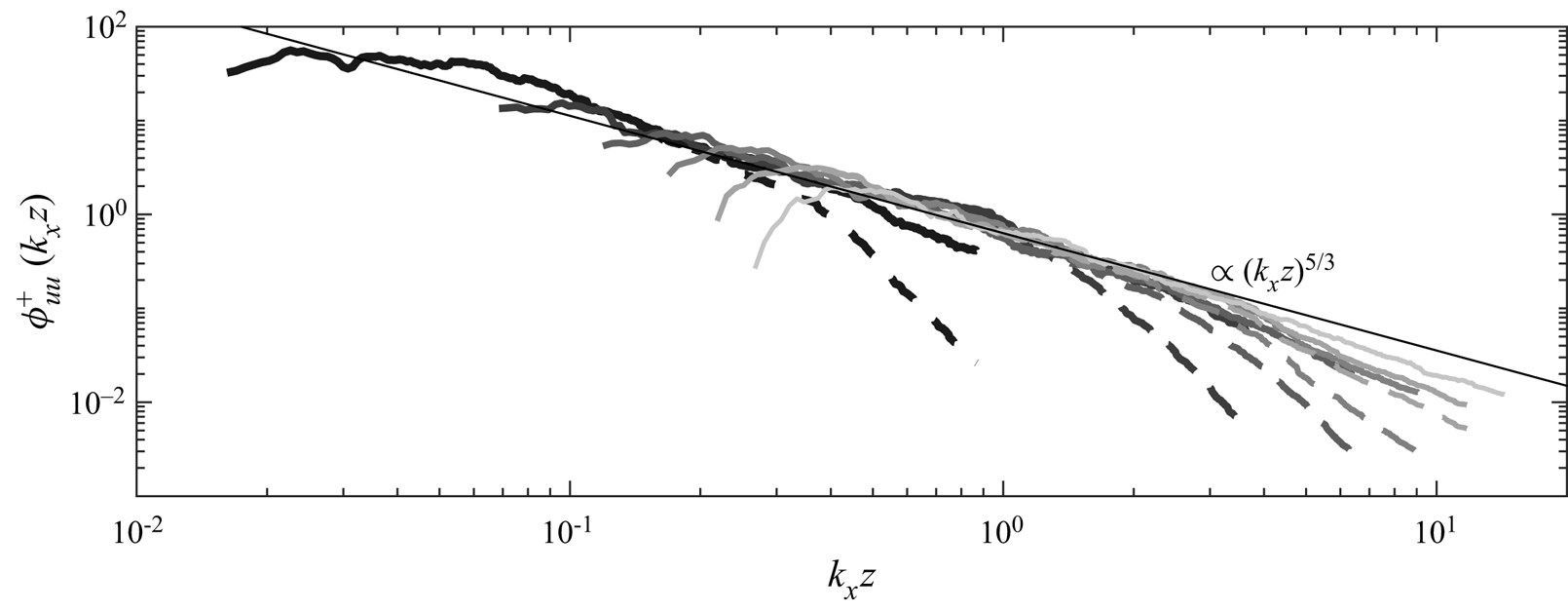
Figure 17. Correction of the streamwise velocity energy spectra obtained from the LiDAR measurements at six different wall-normal positions equally spaced between 6 and 121 m, respectively. Lines become darker with increasing height. Continuous lines represent corrected spectra, while dashed lines report raw spectra.
For the lowest part of the ASL ( $z< l$), it should be noted that the present correction method still underestimates the spectral energy, as the
  $k_x^{-1}$ region is also affected by the LiDAR spatial averaging. Other spectral correction procedures were tested (Mann et al. Reference Mann, Cariou, Courtney, Parmentier, Mikkelsen, Wagner, Lindelöw, Sjöholm and Enevoldsen2009; Cheynet et al. Reference Cheynet, Jakobsen, Snæbjörnsson, Mann, Courtney, Lea and Svardal2017), while the data-driven method of Puccioni & Iungo (Reference Puccioni and Iungo2021) provided the largest variance recovery.
Appendix C. Smoothing of the LCS
The parameters for the Welch spectral estimator (Welch Reference Welch1967), namely window length and overlapping, used for the calculation of the LCS are firstly determined by leveraging a synthetic first-order autoregressive model,  $q_n$, defined as (Von Storch & Zwiers Reference Von Storch and Zwiers1999)
 \begin{equation} q_n = \left\{\begin{array}{@{}ll} e_n & \text{as}\ n=1, \\ \alpha q_{n-1} + e_n & \text{as}\ n>1, \end{array}\right. \end{equation}
where  $e_n$ is a white-noise Gaussian process with variance
  $\sigma _e^2$,
  $0<\alpha <1$ and
  $n=1,\ldots,M$. From (C1) a second synthetic signal can be defined as
 \begin{equation} s_n = \beta q_n + \tilde{e}_{n}, \end{equation}
where  $\tilde {e}_{n}$ is another white-noise Gaussian process with variance
  $\tilde {\sigma }_{e}^2$, and
  $0<\beta <1$. From the definition of auto- and cross-spectra, it is possible to show that the coherence between
  $q$ and
  $s$ is given by
 \begin{equation} \gamma^2(q,s;f)=\frac{\beta^2\phi_{qq}(\,f)}{\beta^2\phi_{qq}(\,f)+ \tilde{\sigma}_{e}^2}, \end{equation}
where  $f$ is the frequency and
 \begin{equation} \phi_{qq}(\,f) = \frac{\sigma_e^2}{1+\alpha^2-2\alpha\cos(2{\rm \pi} f)}. \end{equation}
Thus, leveraging these two related autoregressive signals  $q_n$ and
  $s_n$, a theoretical reference for the LCS is available against which the numerical algorithm for the evaluation of the LCS from the two signals can be assessed.
As previously mentioned, the coherence for two time series is calculated by means of the Welch (Reference Welch1967) algorithm; the ensemble averaging operation in (3.15) is simulated by dividing the entire signals into a certain number of sub-windows,  $n_W$, with a certain overlapping percentage. Successively, a moving average with stencil
  $f_n\pm 0.35f_n (n=1,\ldots,M)$ is performed to smooth the LCS (Baars et al. Reference Baars, Hutchins and Marusic2017; Baars & Marusic Reference Baars and Marusic2020a).
The algorithm for the calculation of the LCS between the discrete signals of (C1) and (C2) is tested, then the results are compared against the analytical LCS reported in (C3). The results obtained from this sensitivity study are reported in figure 18 using  $\alpha =0.9, \beta =0.3$ for a signal with
  $M=3600$ samples simulated with a sampling frequency of
  $1$ Hz. A close agreement between the numerical results and the analytical prediction is obtained for the case with
  $n_W=20$ and
  $90\,\%$ overlapping (figure 18f), which are the parameters used for the present work.
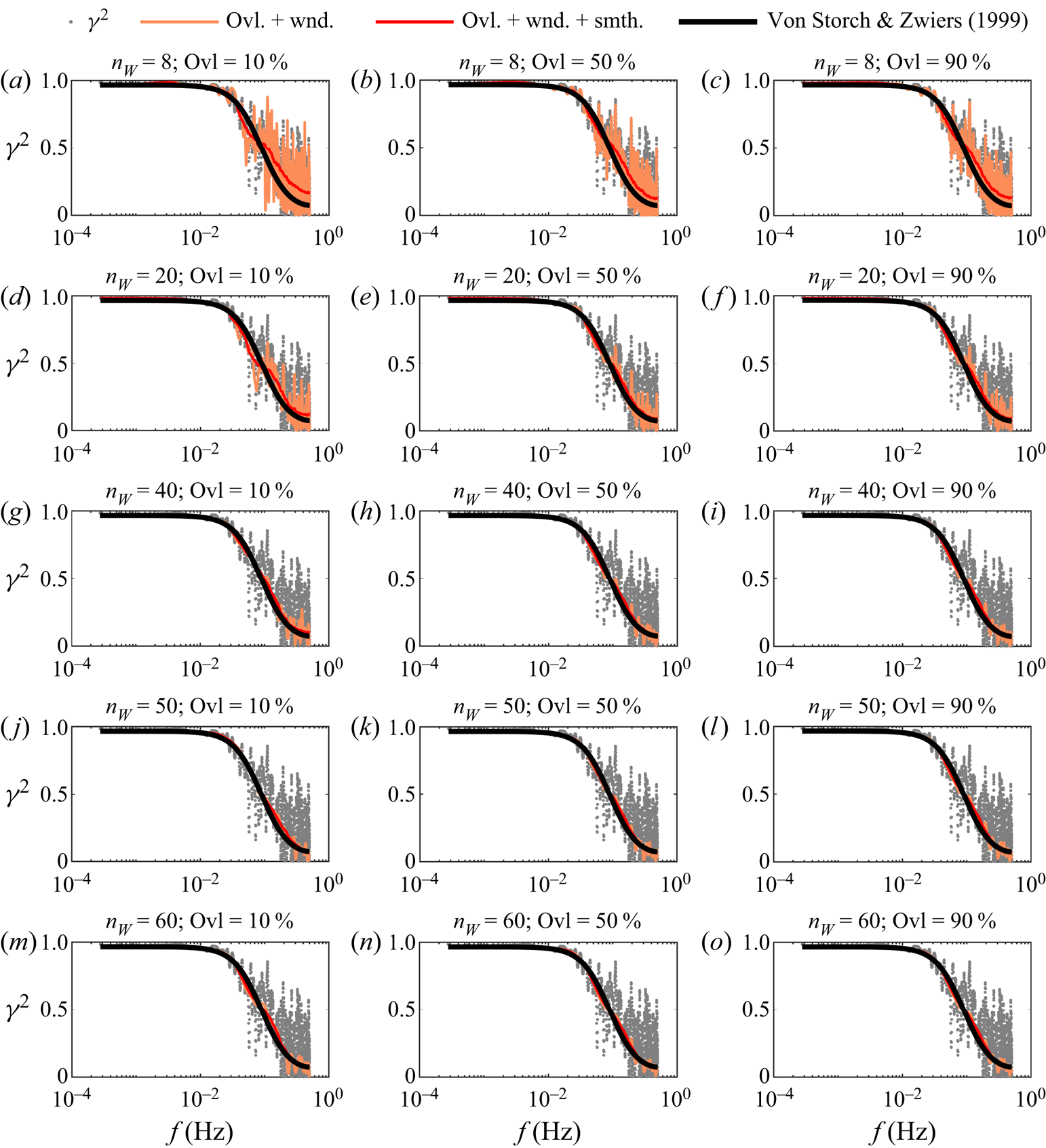
Figure 18. Sensitivity of the LCS to the windowing and overlapping parameters for a synthetic autoregressive case. Grey dots report the LCS without smoothing, the orange lines depict  $\gamma ^2$ calculated with the Welch (Reference Welch1967) periodogram with the indicated windowing and smoothing parameters, the red lines reports the result after the smoothing procedure and the black lines are the theoretical distribution of Von Storch & Zwiers (Reference Von Storch and Zwiers1999).


 Open access