


1. Introduction
Owing to their technological significance, turbulent boundary layers have, and continue to be, the subject of intense study (Klewicki Reference Klewicki2010; Smits, McKeon & Marusic Reference Smits, McKeon and Marusic2011; Vinuesa et al. Reference Vinuesa, Negi, Atzori, Hanifi, Henningson and Schlatter2018). For the purposes of clarifying the simplest and most fundamental properties of the turbulent boundary layer, the vast majority of studies have focused on the flat plate turbulent boundary layer where there is no streamwise pressure-gradient (PG) (i.e. the zero pressure-gradient turbulent boundary layer (ZPG TBL)). Rarely, however, is the canonical ZPG TBL precisely encountered in practical applications. Indeed, while many applications involve nominally ZPG TBLs (e.g. TBL flow on a commercial aircraft fuselage), many others involve streamwise PGs that have a leading-order dynamical effect. For the purposes of modelling and conceptual understanding, it is thus useful to know those aspects of PG boundary layers that are describable as an extension of those found in the canonical flow. Toward this aim, the present study broadly seeks to clarify the connections between the inertial sublayer of TBLs subjected to moderately adverse pressure-gradients (APG) and the inertial sublayer (logarithmic layer) of the ZPG TBL.
As a starting point, it is useful to consider time scales relevant to the underlying physics. In the case of the ZPG TBL, the two important time scales are the viscous diffusion time,  $t_\nu = \nu /u_\tau ^2$, that is relatively small and representative of the inner region, and $t_{\varDelta } = \varDelta /u_\tau$, a much larger outer region time scale. Here, $\nu$ is the kinematic viscosity of the fluid, $u_\tau$ is the friction velocity ( $\equiv \sqrt {\tau _w/\rho }$, where $\tau _w$ is the mean wall shear stress and $\rho$ the fluid density) and $\varDelta =\int _0^\infty u_\tau ^{-1} (U_\infty -U(y))\,{{\rm d} y}$ is the Rotta–Clauser length scale. In these expressions $U(y)$ is the mean streamwise velocity (a function of the distance-from-the-wall, $y$, at any given $x$) and $U_\infty$ is the free stream velocity (e.g. Tennekes & Lumley Reference Tennekes and Lumley1972). Accordingly, the non-dimensional parameter that describes the ZPG TBL is the ratio of the outer to the inner time scales:
 \begin{equation} Re_\varDelta \equiv \frac{t_\varDelta}{t_\nu} = \frac{\Delta u_\tau}{\nu}. \end{equation}
 Note that for a given flow this is equivalent to the usual friction Reynolds number,  $Re_\tau \equiv \delta u_\tau /\nu$ because $\varDelta$ is a constant fraction of the ‘usual’ TBL thickness $\delta$, i.e. $\varDelta \approx 3.5 \delta$, see for example Morrill-Winter, Philip & Klewicki (Reference Morrill-Winter, Philip and Klewicki2017). A ZPG TBL is deemed to be ‘self-preserving’, as its Reynolds number ( $Re_\tau$ or $Re_\varDelta$) is only slowly varying in space, and the local state of the momentum transport across the flow is reflected by (scales with) the wall shear stress. Note that ZPG TBLs typically grow slowly with $x$, for example ${\rm d}\delta /{\rm d}x \approx 0.012$ at $Re_\tau =14\,500$ whereas at $Re_\tau \approx 8000\, {\rm d}\delta /{\rm d}x \approx 0.016$ (as shown, respectively, by Chauhan et al. (Reference Chauhan, Philip, De Silva, Hutchins and Marusic2014) and Zimmerman et al. (Reference Zimmerman2019)). The present APG TBL measurements for $7100 \leq Re_\tau \leq 7770$ grow at a slightly faster rate, such that $0.016 \leq {\rm d}\delta /{\rm d}x \leq 0.05$. The definition and calculation of $\delta$ are made precise later.
In the case of an APG TBL, at subsonic speeds the free stream flow decelerates, and therefore there is a new time scale associated with the PG,  $t_{PG} = -{({\rm d}U_\infty /{{\rm d}x})}^{-1}$. This introduces a new non-dimensional number (the Clauser PG parameter):
 \begin{equation} \beta \equiv \frac{t_\varDelta}{t_{PG}} = \frac{\Delta u_\tau^{{-}1}}{-({\rm d}U_\infty/{{\rm d} x})^{{-}1}}. \end{equation}
Therefore, the interaction of the outer and PG scales is strongest when  $\beta =O(1)$. Note that because $u_\tau \varDelta = U_\infty \delta ^*$, where $\delta ^*$ is the displacement thickness, and $U_\infty ({\rm d}U_\infty /{{\rm d} x}) = -\rho ^{-1} ({\rm d}P/{{\rm d} x})$, one can also write
 \begin{equation} \beta \equiv \frac{\delta^*}{\tau_w}\frac{{\rm d}P}{{\rm d} x}. \end{equation}
As such, self-preserving APG TBLs are characterized by nominally constant  $\beta$ and $Re_\tau$, (e.g. Townsend Reference Townsend1956; Tennekes & Lumley Reference Tennekes and Lumley1972). Herein we consider experimental measurements of mild APG flows where $Re_\tau$ is large and both $Re_\tau$ and $\beta$ are changing rather slowly. The data analyses also consider large-eddy simulation (LES) data of APG flows for constant $\beta$. As seen in various experimental and numerical APG TBL studies, near or at separation $\beta$ can reach values greater than 10 (e.g. Skåre & Krogstad Reference Skåre and Krogstad1994; Krogstad & Skåre Reference Krogstad and Skåre1995; Hickel & Adams Reference Hickel and Adams2008; Maciel et al. Reference Maciel, Wei, Gungor and Simens2018). In the present paper, however, the cases studied have much smaller $\beta$ values, i.e. $\beta \leq 2$. Thus, for all of the flows studied herein history effects are expected to have only a relatively small influence on the dynamical structure.
1.1. Inertial sublayer
In classical theory the boundary layer is separated into an inner and outer region that overlap across the logarithmic layer (e.g. Tennekes & Lumley Reference Tennekes and Lumley1972). The inner region, where the length scale is order  $\nu /u_\tau$, can be defined by the validity of the law of the wall:
 \begin{equation} U^+{=}\frac{U}{u_{\tau}} =f(y^+) ; \quad y^+{=} \frac{y u_{\tau}}{\nu}. \end{equation}
Here the plus superscript  $(^+)$ denotes normalization by $\nu$, and $u_{\tau }$. The outer region, where the length scale is typically the boundary layer thickness, $\delta$, is described by the defect law
 \begin{equation} \frac{U_\infty-U}{u_{\tau}} = F(\eta) ;\quad \eta = \frac{y}{\delta}. \end{equation}
It is assumed that there is an overlap region where both (1.4) and (1.5) are valid. By matching the velocity gradients of (1.4) and (1.5) we find the logarithmic law
 \begin{equation} \frac{U}{u_{\tau}} = \frac{1}{\kappa} {\rm{ln}}\left(\frac{y u_{\tau}}{\nu}\right) + B, \quad {\rm{or}}, \quad U^+{=} \frac{1}{\kappa} {\rm{ln}}(y^+) + B. \end{equation}
While a topic of continuing study, the values of the constants in (1.6) are  $\kappa \approxeq 0.39$ and $B \approxeq 4.4$ (e.g. Österlund et al. Reference Österlund, Johansson, Nagib and Hites2000; Perry, Hafez & Chong Reference Perry, Hafez and Chong2001; Hellstedt Reference Hellstedt2003; Marusic et al. Reference Marusic, Monty, Hultmark and Smits2013). Under this construction, the start of the overlap layer is order $\nu /u_\tau$ and the logarithmic layer is defined empirically as the point where the profile exhibits an approximately logarithmic variation (e.g. Pope Reference Pope2000). Thus, under this classical description of the ZPG TBL the logarithmic layer is taken empirically (from relatively low Reynolds number data) to extend from $y^+\simeq 30$ to $y/\delta \simeq 0.15$ (e.g. Tennekes & Lumley Reference Tennekes and Lumley1972; Pope Reference Pope2000).
The bounds of the logarithmic layer (or more precisely the inertial sublayer) can, however, also be discerned through an analysis of the mean momentum balance (MMB). The basis for this approach was first described by Wei et al. (Reference Wei, Fife, Klewicki and McMurtry2005) for the ZPG TBL, channel and pipe flows. Here, the regions of the boundary layer are defined by the leading-order forms of the MMB. In these flows, the ratio of the viscous force (VF) term to the turbulent inertia (TI) term of the MMB facilitates identifying the different regions of the flow and their leading-order structure. The onset of the inertial domain is thus rationally defined as the point where the VF term loses leading-order dominance. The MMB analysis of the canonical wall-flows reveals that the  $y^+$ onset of the inertial region is a function of the square root Reynolds number and occurs near $y^+= 3 \sqrt {\delta ^+}$, (Wei et al. Reference Wei, Fife, Klewicki and McMurtry2005; Klewicki, Fife & Wei Reference Klewicki, Fife and Wei2009; Klewicki Reference Klewicki2013; Marusic et al. Reference Marusic, Monty, Hultmark and Smits2013; Morrill-Winter et al. Reference Morrill-Winter, Philip and Klewicki2017), and therefore not at $y^+ \simeq 30$ as traditionally supposed. Herein, $\delta ^+ \equiv \delta _{99} u_\tau /\nu$ and $Re_\tau$ are used interchangeably.
When compared with the ZPG TBL there are significant uncertainties regarding the bounds of the logarithmic layer in the APG TBL. This is at least partially due to the increasing wake strength of the mean velocity profile (Samuel & Joubert Reference Samuel and Joubert1974; Nagano, Tsuji & Houra Reference Nagano, Tsuji and Houra1998; Aubertine & Eaton Reference Aubertine and Eaton2005). Under APG conditions, but at relatively low Reynolds number, observations suggest that the wake layer of the mean velocity profile encroaches on the logarithmic layer from the outer region (e.g. Monty, Harun & Marusic Reference Monty, Harun and Marusic2011). As described later herein, this connects to the free stream balance between the PG and mean advection terms in the mean momentum equation. In the ZPG TBL at sufficiently large Reynolds number, the mean velocity variation with wall-normal distance within the inertial sublayer is given by the logarithmic law to within a very close approximation. With the addition of sufficiently large APG the mean velocity profile has been observed to fall below that given by (1.6) with the noted parameters (e.g. Spalart & Watmuff Reference Spalart and Watmuff1993; Nagano et al. Reference Nagano, Tsuji and Houra1998; Lee & Sung Reference Lee and Sung2008; Monty et al. Reference Monty, Harun and Marusic2011). It has also been observed, however, that the classical logarithmic variation and offset (as described by  $\kappa$ and $B$) are largely preserved in the APG TBL, with the effect of PG essentially manifest in a clear increase in wake strength (Aubertine & Eaton Reference Aubertine and Eaton2005). On the other hand, both Nickels (Reference Nickels2004) and Nagib & Chauhan (Reference Nagib and Chauhan2008) propose that the value of $\kappa$ and $B$ vary depending on the strength of the APG. Various authors have also suggested that the inertial sublayer mean profile can be described by a half-power law as initially proposed by Stratford (Reference Stratford1959). Stratford (Reference Stratford1959) postulates that at separation and closer to the wall the velocity is proportional to the square root of the distance from the wall. This result stems from the assumption that the mixing length is ‘proportional to the distance from the wall’. In connecting the log- and power-law, Brown & Joubert (Reference Brown and Joubert1969) proposed that there is an inner logarithmic region defined by (1.6) with the classical parameters, and an outer region defined by a half-power law. Expanding on these ideas, Knopp et al. (Reference Knopp, Schanz, Schröder, Dumitra, Cierpka, Hain and Kähler2014) suggest that the inner region of the inertial sublayer follows (1.6), but with varying $\kappa$ and $B$, and that the outer inertial sublayer can be described by a modified log-law. This modified log-law reduces to the half-power law of Stratford (Reference Stratford1959) for large PGs. This description is supported by the findings of Knopp et al. (Reference Knopp, Reuther, Novara, Schanz, Schülein, Schröder and Kähler2021), where logarithmic behaviour is observed in the mean velocity profile at large $\beta$ and high Reynolds number, but with a reduced $\kappa$. The extent of this region is also observed by Knopp et al. (Reference Knopp, Reuther, Novara, Schanz, Schülein, Schröder and Kähler2021) to be smaller in comparison with the logarithmic region of the ZPG TBL. A half-power law (the modified log-law of Knopp et al. Reference Knopp, Schanz, Schröder, Dumitra, Cierpka, Hain and Kähler2014) is seen to emerge above the flow domain, where the typical ZPG TBL logarithmic layer would exist. Herein we investigate an approach for locating the bounds of the inertial sublayer that does not depend on $\kappa$ and $B$. Furthermore, the uncertainty in the location and properties of the inertial layer is exacerbated by the fact that there is dependence on both $\beta$ and $Re_\tau$, and most data, although available over a range of $\beta$, are at relatively low $Re_\tau$. The present larger $Re_\tau$ experimental data alleviate some of these issues.
Central to the mean velocity profile log-law and the structure of turbulence in the ZPG TBL is the idea of ‘distance-from-the-wall’ scaling (e.g. Townsend Reference Townsend1976; Wei et al. Reference Wei, Fife, Klewicki and McMurtry2005; Baidya et al. Reference Baidya, Philip, Hutchins, Monty and Marusic2017). ‘A classical’ but less rigorous mixing length argument suggests that the stress velocity scale (i.e. square root of the Reynolds shear stress (RS)) is proportional to  $y {\rm d}U/{{\rm d}y}$, where $y$ – the distance-from-the-wall – is the mixing length. For a region with constant stress, this gives the log-law in $U$. More rigorous arguments by Morrill-Winter et al. (Reference Morrill-Winter, Philip and Klewicki2017) that eventually lead to a log-law also show that the appropriate length scale within the flow follows a $y$-scaling. Although the concept of distance-from-the-wall is well appreciated for the ZPG TBL, it has perhaps received less attention in APG TBL flows.
Stratford's (Reference Stratford1959) half-power law  $U$-profile relies on a $y$-scaling of the mixing length. In fact, Stratford (Reference Stratford1959) shows that if the RS $\propto (y\,{\rm d}U/{{\rm d} y})^2$, and in APG flow since stress is also $\propto y\, {\rm d}P/{{\rm d} x}$ (from the mean momentum equation, cf. equation (2.7)), it follows that ${\rm d}U/{{\rm d} y} \propto y^{-1/2}\sqrt {{\rm d}P/{{\rm d} x}}$, or $U \propto y^{1/2}\sqrt {{\rm d}P/{{\rm d} x}}$, which is Stratford's (Reference Stratford1959) half-power law. Although based on an heuristic mixing length argument, what is highlighted here is that both log-law (in ZPG flow) and a power-law (in APG flows) are commensurate with the distance-from-the-wall scaling. A part of the present study focuses on presenting a more rigorous theoretical argument for $y$-scaling in APG flows (following on from Fife, Klewicki & Wei (Reference Fife, Klewicki and Wei2009)), and providing experimental support from high $Re_\tau$ spectral maps, where length scales appear naturally.
1.2. Present study
The main aims of the present study centre on the inertial sublayer of the APG TBL and the degree to which its characteristics are similar to those of the ZPG TBL. For the remainder of this paper the inertial sublayer is defined as the region between where the VF term has lost leading order and where the streamwise kurtosis has reached the Gaussian value of 3. This study focuses on four traits of the inertial sublayer: (1) logarithmic behaviour in the mean velocity profile; (2) position of the inertial sublayer in relation to the RS,  $\overline {uv}$ profile; (3) properties of the turbulent stresses, including the decay of the streamwise velocity fluctuation variances, $\overline {u^2}$; and (4) the distance-from-the-wall scaling of various turbulence properties. For the remainder of this paper these will be denoted by traits (1)–(4), and various approaches, both equation-based analyses and empirical, are used to describe and quantify these inertial sublayer characteristics.
The logarithmic behaviour of the mean velocity profile is investigated using empirical measures such as the indicator function. The indicator function  $\varXi \equiv y^+({\rm d}U^+/{{\rm d} y}^+$) is commonly used to evaluate whether, and locate where, the mean velocity profile (approximately) exhibits logarithmic dependence. This function is commonly used to analyse ZPG flows, but has also been used to study APG flows (e.g. Monty et al. Reference Monty, Harun and Marusic2011). Such empirical measures are complemented by mean equation analyses. These analyses are founded in the MMB and related quantities associated with its once-integrated form (e.g. the stress balances). The stress balance analysis herein clarifies that logarithmic dependence in the mean profile can be characterized as stemming from the sum of the inertial terms of the stress balance yielding a subdominant (residual) ${\rm d}U^+/{{\rm d} y}^+$ that varies like $1/y^+$. Analytical predictions that enjoy empirical support indicate that in the ZPG TBL the onset of the inertial sublayer nominally coincides with the peak of the RS (Wei et al. Reference Wei, Fife, Klewicki and McMurtry2005; Klewicki et al. Reference Klewicki, Fife and Wei2009). This spatial coincidence is shown herein to not hold in the APG TBL. Unlike in the ZPG TBL, it is also revealed that the inertial sublayer in the APG TBL is not characterized by a logarithmic $\overline {u^2}$ decay. It is, however, also shown that the peak in $-\overline {uv}$ still aligns with the final decay of $\overline {u^2}$ for both the ZPG TBL and APG TBL. Stress-balance-based analyses are then augmented through analysis of the MMB – the $y$-derivative of the stress balance. This analysis shows that the curvature of the VF term of the APG TBL maintains certain properties that are held in common with those of the ZPG TBL. The scaling patch analysis of Fife et al. (Reference Fife, Klewicki and Wei2009) tells us that if the mean dynamics on the inertial sublayer become self-similar (e.g. through increased insulation from boundary condition effects) and that there is a single velocity scale, then this will coincide with distance-from-the-wall scaling. It is, however, also possible to have $y$-scaling with non-constant velocity scales, as discussed in the Appendix (A). Evidence of this is given for the APG TBL, and spectral analyses are used to investigate the existence of distance-from-the-wall-scaling more deeply.
2. Attributes of the inertial layer
2.1. Indicator function
The indicator function  $\varXi$ is used to observe whether the mean velocity profile exhibits a logarithmic behaviour. If a logarithmic layer does exist, then there will be a range of $y^+$ over which the $\varXi$ becomes nominally constant. In ZPG flows this region is located between $y^+\simeq 3\sqrt {\delta ^+}$ and $y/\delta \simeq 0.15$ (Wei et al. Reference Wei, Fife, Klewicki and McMurtry2005; Marusic & Adrian Reference Marusic and Adrian2013; Morrill-Winter et al. Reference Morrill-Winter, Philip and Klewicki2017). The indicator functions of the present APG flows are examined relative to these bounds.
2.2. MMB
The MMB is the Reynolds-averaged streamwise Navier–Stokes equation. We first consider the MMB for channel flow since its force balance structure contains a PG term that is the sole driving force of the fluid motion (see Wei et al. Reference Wei, Fife, Klewicki and McMurtry2005; Fife et al. Reference Fife, Klewicki and Wei2009; Klewicki Reference Klewicki2013). For channel flows the mean equation is a balance of three terms: VF; TI; PG. The inner-normalized form of this equation is given by
 \begin{equation} \underbrace{\frac{\partial^2 U^+}{\partial {y^2}^+}}_{\text{VF}} + \underbrace{\vphantom{\frac{\partial^2 U^+}{\partial {y^2}^+}}\frac{-\partial \overline{uv}^+}{\partial y^+}}_{\text{TI}} + \underbrace{\vphantom{\frac{\partial^2 U^+}{\partial {y^2}^+}}\frac{1}{{\delta}^+}}_{\text{PG}} = 0. \end{equation}
Here the VF term is the gradient of the viscous stress (VS) and the TI term is the gradient of the RS. The zero crossing of the TI term coincides with the peak location of the RS. On the wall-ward side of this zero crossing, TI is positive and acts as a momentum source, whereas beyond the zero crossing, the TI term becomes negative and acts as a momentum sink. The PG term is only a function of Reynolds number and remains constant with wall-normal distance.
For the two-dimensional ZPG TBL the equation is still a balance of three terms. Here, the PG term of the channel is supplanted by the mean inertia (MI) term, which is still a function of Reynolds number, but is no longer constant in  $y^+$ or streamwise distance $x^+$,
 \begin{equation} \underbrace{\vphantom{\left[{-}U^+\frac{\partial U^+}{\partial x^+}-V^+\frac{\partial U^+}{\partial y^+}\right]} \frac{\partial^2 U^+}{\partial {y^2}^+}}_{\text{VF}} + \underbrace{\vphantom{\left[{-}U^+\frac{\partial U^+}{\partial x^+}-V^+\frac{\partial U^+}{\partial y^+}\right]} \frac{-\partial \overline{uv}^+}{\partial y^+}}_{\text{TI}} + \underbrace{\left[{-}U^+\frac{\partial U^+}{\partial x^+}-V^+\frac{\partial U^+}{\partial y^+}\right]}_{\text{MI}} = 0. \end{equation}
Near the wall (but beyond a few viscous lengths from the wall) in either the channel or boundary layer, the VF and TI terms are dominant. Because of this, the MMB structure for the ZPG TBL and channel flow is very similar. The main difference is that small outer peaks form in the MI and TI terms of the ZPG TBL. For both the ZPG TBL and channel flow, the onset of the inertial sublayer scales with  $\sqrt {\delta ^+}$. Within the context of the MMB-based framework, the onset of the inertial sublayer is defined as where the VF loses leading order. This nominally corresponds to the location where the TI term crosses zero.
The MMB for the modest  $\beta$ APG TBL contains four terms. (Note that under large APG, the turbulence contributions to the advective term become non-negligible, see for example Castillo & George (Reference Castillo and George2001).) Like in the case of the ZPG TBL, this equation includes a non-constant MI term, and like in the channel case the relevant equation also includes a constant PG term. Where all terms are positioned on the left, for the APG TBL the PG term is constant and negative, while for channel flow it is positive,
 \begin{equation} \underbrace{\vphantom{\left[{-}U^+\frac{\partial U^+}{\partial x^+}-V^+\frac{\partial U^+}{\partial y^+}\right]} \frac{\partial^2 U^+}{\partial {y^2}^+}}_{\text{VF}} + \underbrace{\vphantom{\left[{-}U^+\frac{\partial U^+}{\partial x^+}-V^+\frac{\partial U^+}{\partial y^+}\right]} \frac{-\partial \overline{uv}^+}{\partial y^+}}_{\text{TI}} + \underbrace{\left[{-}U^+\frac{\partial U^+}{\partial x^+}-V^+\frac{\partial U^+}{\partial y^+}\right]}_{\text{MI}} + \underbrace{\vphantom{\left[{-}U^+\frac{\partial U^+}{\partial x^+}-V^+\frac{\partial U^+}{\partial y^+}\right]} U_\infty ^+ \frac{\partial U_\infty ^+}{\partial x^+}}_{\text{PG}} = 0. \end{equation}
 Owing to the additional PG term, the balance changes from that for the ZPG TBL shown in figure 1(a) to that for the APG TBL shown in figure 1(b). For the APG TBL, the VF term solely balances the PG term as the wall is approached, while the PG term comes to identically balance the MI term in the free stream. Like in the ZPG case, the MI term increases in magnitude as the VF term loses leading order (e.g. near where the VF is less than 25 % of the balance). As previously mentioned, the position in the ZPG TBL flow where the VF term loses leading order nominally coincides with where the TI term crosses zero, as both  $y^+$ positions scale with $\sqrt {\delta ^+}$. In the APG TBL flow, however, the TI term crosses zero well-beyond where the VF term loses dominance, as seen more clearly in figure 2. In the region where the VF loses leading order the TI term maintains nominally the same shape as in the ZPG case, but is shifted upwards. Here, subtle changes due to the MI term are, however, visible. Beyond the location where the VF term approaches zero, a new inertial balance emerges. This delicate balance involves all three of the remaining terms, the TI, MI and PG terms.

Figure 1. (a) The MMB of ZPG TBL at  $Re_\tau = 490$, data set from Schlatter & Örlü (Reference Schlatter and Örlü2010). (b) The MMB of APG TBL at $Re_\tau = 490$ at $\beta =1$, data set from Bobke et al. (Reference Bobke, Vinuesa, Örlü and Schlatter2017).

Figure 2. The MMB in the inertial sublayer at  $Re_\tau =490$. The ZPG TBL case plotted with dark thin lines and APG TBL at $\beta =1$, from Bobke et al. (Reference Bobke, Vinuesa, Örlü and Schlatter2017) plotted with thick lines in lighter shades. Zero crossing of the TI term marked by orange thick circle.
Overall, the results of figures 1 and 2 indicate that if the beginning of the inertial sublayer in the APG flow is marked by the loss of a leading-order VF term (as it is in the ZPG flow), then the inertial balance on this sublayer is more complex than in the ZPG TBL. Because of this, the TI zero crossing is, for example, no longer a signature of entering onto the inertial sublayer. Physically, this means that the turbulent motions do not necessarily behave like a momentum sink on the inertial sublayer. It similarly indicates that features other than the TI zero crossing constitute the essential mathematical attributes that define the inertial sublayer.
Self-similar mean dynamics admitted by the MMB and distance-from-the-wall scaling are compatible concepts. Analytical developments indicate that say if the ‘natural’ length scale of the flow varies as distance-from-the-wall and the velocity scale is constant (e.g.  $u_\tau$), then there is a logarithmic layer, as shown in Fife et al. (Reference Fife, Wei, Klewicki and McMurtry2005) via a rescaling of the MMB and an analysis of scale hierarchies in wall-bounded turbulent flows.
For APG TBLs, and following the framework of Fife et al. (Reference Fife, Wei, Klewicki and McMurtry2005, Reference Fife, Klewicki and Wei2009) for channel flows, the Appendix (A) shows that a modified RS term  $T_\epsilon ^{+}$ can be constructed. Note that $\epsilon$ is a subscript on $T^+ \equiv -{\overline {uv}}^+$ to indicate the modified RS function. Similar to the analysis carried out for channel and ZPG TBL flows, we introduce the small parameter $\epsilon$ whose values (within a specified range) are each associated with a ‘scaling patch’. (See, the Appendix (A.1) for the definition of a scaling patch.) For APG TBLs the modified RS takes the following form:
 \begin{equation} T_\epsilon^{+}(y^+) = T^+(y^+) + \displaystyle\int_{0}^{y^+}\text{MI}({y^\prime}^+)\,{\rm d}{y^\prime}^+ + (\text{PG} - \epsilon )y^+. \end{equation}
As  $PG\to 0$, (2.4) reduces to the form given in Morrill-Winter et al. (Reference Morrill-Winter, Philip and Klewicki2017) for the ZPG TBL. The MMB can then be written as
 \begin{equation} \frac{\partial^2U^+}{\partial{y^+}^{2}}+ \frac{\partial T_\epsilon^{+}}{\partial y^+} + \epsilon = 0. \end{equation}
As discussed in more detail in the Appendix (A), (2.5) can then be made parameterless (see the steps to transform equation (A2) into (A6)),
 \begin{equation} \frac{\partial^2\hat{U}}{\partial \hat{y}^{2}} + \frac{\partial \hat{T}}{\partial \hat{y}} + 1 = 0, \end{equation}
where  $\hat {\cdot }$ denotes normalization by the characteristic or ‘natural’ velocity and length. On each of these scaling patches, the MMB reduces to an invariant form.
Continuing further from (2.6), the Appendix (A) clarifies the possibility and consequences of multiple or a hierarchy of velocity scales represented within the boundary layer (and not a single velocity scale such as  $u_\tau$). Under these conditions the logarithmic $U^+$ is not necessarily present, rather the mean velocity could admit a power-law, but for which distance-from-the-wall scaling could still hold. Such a condition is a distinct possibility for APG flows. As such, this analysis provides some credibility to Stratford's (Reference Stratford1959) heuristic use of distance-from-the-wall scaling in the APG TBL. Identifying the appropriate velocity scale for APG flows, however, is beyond the scope of this paper. Instead, primary interests are on examining whether distance-from-the-wall scaling is seen via empirical means and on discerning how appropriate the friction velocity is for scaling APG TBLs. The theoretical basis for these arguments and an explanation of scale hierarchies following Fife et al. (Reference Fife, Klewicki and Wei2009) is discussed in the Appendix (A).
2.3. Stress balance
The properties of the once-integrated form of (2.3) are used to further clarify inertial layer properties. A single integration of the MMB from the wall to a particular  $y^+$ location yields a balance of stresses. The inner-normalized balance of stresses for the APG TBL becomes
 \begin{equation} \underbrace{\vphantom{\displaystyle\int_0^{y^+} \left[{-}U^+\frac{\partial U^+}{\partial x^+}-V^+\frac{\partial U^+}{\partial {y^\prime}^+}\right]d{y^\prime}^+} \frac{\partial U^+}{\partial {y}^+}}_{{\text{VS}} = \int\text{VF}} + \underbrace{\vphantom{\displaystyle\int_0^{y^+} \left[{-}U^+\frac{\partial U^+}{\partial x^+}-V^+\frac{\partial U^+}{\partial {y^\prime}^+}\right]d{y^\prime}^+} (-\overline{uv}^+)}_{{\text{RS}} = \int\text{TI}} + \underbrace{\displaystyle\int_0^{y^+} \left[{-}U^+\frac{\partial U^+}{\partial x^+} -V^+\frac{\partial U^+}{\partial {y^\prime}^+}\right]\,{\rm d}{y^\prime}^+}_{{\text{MIS}} = \int\text{MI}} + \underbrace{\vphantom{\displaystyle\int_0^{y^+} \left[{-}U^+\frac{\partial U^+}{\partial x^+}-V^+\frac{\partial U^+}{\partial {y^\prime}^+}\right]d{y^\prime}^+} ({-}y^+P_x^+)}_{{\text{PS}} = \int\text{PG}} = 1, \end{equation}
where  $-P_x^+\equiv U_\infty ^+ (\partial U_\infty ^+/\partial x^+)$ and $y^\prime$ is a dummy variable of integration. The integrated VF term becomes the VS (which reaches unity at $y=0$) and the integrated TI term becomes the RS. The stress balance for the ZPG TBL and APG TBL are shown in figures 3(a) and 3(b), respectively. Here, the focus is on the behaviour of the stress balance in the region where the VF loses leading order. For the ZPG case, the VS term decays as $(\kappa y^+)^{-1}$, which is associated with a logarithmic mean velocity. While the behaviour of the VS term for the present measurements is of interest, it is, however, difficult to obtain accurate estimates of the VS (or mean inertia stress (MIS)) term from experimental measurements. This is because VS becomes very small away from the wall relative to other terms (which are $O(1)$ in this region). On the other hand, the RS and PG can be measured with reasonable accuracy. By observing the remaining terms in the stress balance, such as the pressure stress and RS, this behaviour can be examined in greater detail.

Figure 3. (a) Stress balance of ZPG TBL at  $Re_\tau = 490$, data set from Schlatter & Örlü (Reference Schlatter and Örlü2010). (b) Stress Balance of APG TBL at $Re_\tau = 490$ at $\beta =1$ data set from Bobke et al. (Reference Bobke, Vinuesa, Örlü and Schlatter2017).
2.4. Higher-order statistics
The RS, variance, kurtosis and skewness of the fluctuating velocities,  $u$ and $v$, will be used to better understand the outer bound of the inertial sublayer. In the ZPG TBL the peak in the RS nominally corresponds with the onset of the inertial sublayer. In ZPG TBLs at sufficiently large $Re_\tau$, the variance of $u$ exhibits a logarithmic decay with $y$ on the same domain where $U^+$ varies logarithmically (e.g. Marusic et al. Reference Marusic, Monty, Hultmark and Smits2013). The kurtosis profiles of both $u$ and $v$ exhibit an outer peak that reflects the turbulent/non-turbulent intermittency in the boundary layer (e.g. Klebanoff Reference Klebanoff1955). This outer peak, and large kurtosis values in general, indicate that the instantaneous fluctuations tend to be either much smaller or much larger in magnitude than the standard deviation. Consistently, the $u$ skewness exhibits large negative values as the free stream is approached. Here the probability of large excursions exceeding the mean become diminishingly small, while those below the mean are comparatively common. Comparison of these statistics in the present APG flows thus provides a measure, relative to the ZPG flow, of how deeply the outer boundary condition influence penetrates into the interior of the flow, thus possibly influencing the upper bound of the inertial layer.
2.5. Spectra
Analyses of the premultiplied (co)spectra  $k_xE$ of $\overline {u^2}$, $\overline {v^2}$ and $\overline {uv}$ are used to identify wall-distance scaling in the inertial sublayer as approximately located using the indicator function. Here, $k_x$ is the streamwise wavenumber and $E$ is the power spectral density, such that integration of $E$ from $k_x = 0$ to $\infty$ will recover the corresponding variance or covariance. Premultiplied spectra evidence wall-distance scaling if their peak locations scale with $y$ over a range of wall-normal locations. The wavelength $\lambda _x = 2{\rm \pi} /k_x$ (or wavelength neighbourhood, as $k_xE$ is a per decade density rather than a per wavenumber density) that contributes the most to the variance and RS, as approximated by the peak in the spectra, is also examined. Wall-distance scaling is seen in the premultiplied spectra in Zimmerman (Reference Zimmerman2019) for ZPG TBLs and pipe flows at $\lambda _x/y = 2$, and these previous results are used to guide our investigation of the APG TBL spectra. The spectral analysis also looks for PG influences on the large scale motions that are observed at $\lambda _x/\delta \simeq 3$ in ZPG TBL flows.
3. Experimental and numerical data sets
3.1. Quantifying the PG
The value of the Clauser PG parameter  $\beta$ distinguishes between the ZPG ( $\beta =0$), APG ( $\beta >0$) and favourable pressure-gradient (FPG) ( $\beta <0$) cases. A boundary layer will behave differently depending on how rapidly $\beta$ is changing and whether $\beta$ is decreasing or increasing with the Reynolds number. Herein the focus is on near-self-preserving cases, where history effects are minimal, i.e. $\beta$ is nominally constant or changing mildly with Reynolds number.
Note that PG can also be quantified by the acceleration parameter,
 \begin{equation} K \equiv \frac{\nu}{U_\infty^2}\frac{{\rm d}U_\infty}{{\rm d}x}. \end{equation}
To provide context and comparison with other researchers who have used the acceleration parameter, the present values of  $K$ are also given in table 1.
Table 1. Summary of present APG TBL experiments, lower Reynolds number APG TBL experiments and LES, and ZPG TBL experiments and DNS. The distance  $x$ (m) is the distance downstream from the start of the APG ramp section. Here Z19 refers to Zimmerman (Reference Zimmerman2019) experiments, V20 refers to Volino (Reference Volino2020) experiments, H13 refers to Harun et al. (Reference Harun, Monty, Mathis and Marusic2013) experiments, SÖ10 refers to Schlatter & Örlü (Reference Schlatter and Örlü2010) DNS and B17 refers to Bobke et al. (Reference Bobke, Vinuesa, Örlü and Schlatter2017) LES.

3.2. Facility and ramp
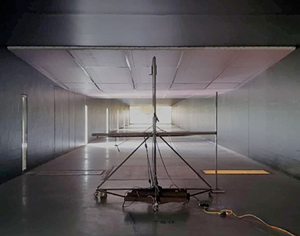
Experiments at relatively large Reynolds numbers were conducted in the Flow Physics Facility (FPF) at the University of New Hampshire. The nominal configuration of the FPF is a ZPG wind tunnel with a  $2.8\,{\rm m} \times 6\,{\rm m}$ cross-section having a fetch of 72 m in the streamwise direction (Vincenti et al. Reference Vincenti, Klewicki, Morrill-Winter, White and Wosnik2013). To create a PG, a ramp structure was installed in the FPF that is nominally based on the experimental design of Aubertine & Eaton (Reference Aubertine and Eaton2005). Unlike the ramp of Aubertine & Eaton (Reference Aubertine and Eaton2005), the present ramp structure was installed on the ceiling of the FPF, instead of the floor. The substantive difference here is that the present measurements were acquired on the flat floor. Thus, they include PG effects but not surface curvature effects. The ramp insert extends approximately 15 m downstream and creates an initial FPG region that reduces the tunnel height by 0.4 m over a 3.1 m streamwise distance. This is followed by a ZPG flat region (where the flow relaxes back to a nearly canonical state) extending approximately 7.0 m downstream. That is then followed by an APG ramp that expands the tunnel height by 0.5 m over a 5.3 m streamwise distance. Downstream of the ramp system the flow develops under ZPG conditions over a fetch of approximate 20 m. The focus of the present study is on the hot-wire measurements acquired along the APG ramp. A schematic of the flow geometry is shown in figure 4. The blue dots indicate the locations where the measurements were acquired.

Figure 4. Current flow geometry and measurement locations. Arrow points in flow direction. Symbols given in table 1.
3.3. Experimental techniques
3.3.1. Pressure distribution
As mentioned above, the pressure distribution was measured along the floor of the wind tunnel. This is different from similar ramp experiments, e.g. Aubertine & Eaton (Reference Aubertine and Eaton2005, Reference Aubertine and Eaton2006) and Cuvier et al. (Reference Cuvier, Foucaut, Braud and Stanislas2014), where the surface pressure was measured directly along the ramp. In their experiments suction peaks were observed near the discontinuous surface transitions between sections of the ramp structure. Besides the suction peaks, the behaviour of the pressure distribution remains essentially the same whether the pressure is measured directly along the ramp or on the opposite surface of the test section, as seen in Cuvier et al. (Reference Cuvier2017). Pitot-static tube measurements were taken 10 cm above the floor of the wind tunnel starting at approximately 15 m upstream of the ramp insert and extending to approximately 17 m downstream of the ramp insert. The coefficient of pressure  $C_p \equiv (P-P_o)/(0.5 \rho U_o^2)$, where $P$ is the local static pressure, $U_o$ is the free stream velocity taken at a reference location, which is at $x_{scaled} =-0.3$. The distance, $x_{scaled}$, is the streamwise distance normalized by the APG ramp length 5.3 m, where $x_{scaled} =0$ is at the start of the APG ramp and $x_{scaled} =1$ is at the end of the APG ramp. The present $C_p$ distribution was compared with that of Aubertine & Eaton (Reference Aubertine and Eaton2005) to confirm that these pressure distributions were nominally the same, see figure 5. The pressure distributions were similar to those reported by Aubertine & Eaton (Reference Aubertine and Eaton2005) except for the aforementioned suction peak. The flow initially accelerates due to the FPG ramp insert causing a strong FPG and subsequently re-establishes a constant free stream velocity along the ZPG portion of the ramp. The presence of the APG ramp detectably influences flow behaviour from approximately $-0.5 \leq x_{scaled} \leq 1.6$. We also note that unlike the studies of Aubertine & Eaton (Reference Aubertine and Eaton2005, Reference Aubertine and Eaton2006) and Cuvier et al. (Reference Cuvier2017) the present set-up features a relatively long flat test section after the FPG section and before the start of the APG section. This ensures approximately ZPG flow (or at worst a very mild FPG) before the APG ramp.

Figure 5. Pressure distribution of the present study (black thick dashed) and of Aubertine & Eaton (Reference Aubertine and Eaton2005) (red thick dashed). On the top  $x$-axis the distance is given in metres where $x=0$ at the start of the APG ramp. On the bottom $x$-axis the distance is normalized by the APG ramp length 5.3 m: $x_{scaled} =0$ is at the start of the APG ramp and $x_{scaled} =1$ is at the end of the APG ramp.
3.3.2. Hot-wire anemometry
An in-house manufactured hot-wire probe capable of measuring the instantaneous streamwise and wall-normal velocities was used, as seen in figure 6. The probe is based on the design of Kawall, Shokr & Keffer (Reference Kawall, Shokr and Keffer1983) and consists of three  $5\,\mathrm {\mu }{\rm m}$ diameter gold-plated tungsten hot-wires: two wires arranged in an $\times$-array are used to discern the streamwise and wall-normal velocities simultaneously and one single wire only measures the streamwise velocity. The gold plating is very thin compared with the overall diameter of the sensing element (i.e. it is not a Wollaston-type wire), and is included only to allow soldered connections between the wire and the supporting prongs. The non-dimensional wire length of the single wire is $L^+ = 17.6$, while the length of the $\times$-array wires projected onto the $y\text {--}z$ plane is $L^+/\sqrt {2}$. The probe's speed response is calibrated in the free stream of the wind tunnel before and after each profile. The angular response of the probe is calibrated via an articulating jet. The calibration process is described in Zimmerman (Reference Zimmerman2019). The raw sensor output is reduced to velocity following the procedure described in Morrill-Winter et al. (Reference Morrill-Winter, Klewicki, Baidya and Marusic2015) for a four-wire hot-wire probe, but adapted here for the three-wire probe. Relative to an $\times$-array alone, the three-wire arrangement reduces the sensitivity of the transverse velocity output to calibration drift of any one sensor relative to a typical two-wire $\times$-array by employing the redundant single wire, see Morrill-Winter et al. (Reference Morrill-Winter, Klewicki, Baidya and Marusic2015).

Figure 6. (a) Front-on probe schematic with relative dimensions. Probe centroid is indicated by the symbol  $\oplus$. The $\times$-array wires mounted on a shorter prong represented by the symbol $\otimes$ and a longer prong represented by the symbol $\odot$. Centre single wire mounted on prongs represented by $\bigcirc$. (b) Front-on picture of actual probe. (c) Side view of probe, schematic. (d) Side view of actual probe.
The non-dimensionalized sample interval for the hot-wire measurements is  $\Delta t_s^+ = (1/f_s)u_\tau ^2/\nu$, where $f_s$ is the sampling frequency. Table 1 lists $\Delta t_s^+$ for the present measurements and those of Zimmerman (Reference Zimmerman2019).
3.3.3. Measurement parameters
The friction velocity  $u_\tau$ was initially estimated by measuring the wall shear stress using 1.4 mm and 2.8 mm diameter Preston tubes ( ${\approx }22$ and 44 viscous lengths in the corresponding ZPG flow, respectively). The PGs are well within the limits proposed by Patel (Reference Patel1965). To check the validity of the Preston tube measurements the hot-wire-based mean velocity profiles were compared with the LES mean velocity profiles of Bobke et al. (Reference Bobke, Vinuesa, Örlü and Schlatter2017). Here the LES data revealed that near the wall the $U^+$ versus $y^+$ profiles for mild $\beta$ APG flows ( $\beta \lesssim 2$) match those of the ZPG direct numerical simulations (DNS) of Sillero, Jiménez & Moser (Reference Sillero, Jiménez and Moser2013) to within ${\pm }7\,\%$ for $y^+\lesssim 40$. Given the similarity between mild $\beta$ APG cases and canonical cases, a method similar to the Clauser chart method for ZPG TBLs was adopted. A second estimation of $u_\tau$ was obtained by matching the hot-wire mean velocity profiles to the LES mean velocity profiles for $y^+<40$. The $u_\tau$ values obtained from this matched-profile method agreed with the $u_\tau$ values obtained via the Preston tube to within ${\pm }8\,\%$. Since the matched profile $u_\tau$ has comparably less scatter with downstream distance, this $u_\tau$ is used herein. This might result in a slight but systematic underestimation of $u_\tau$ (and thus overestimation of $U^+$, etc.), but should not affect our interpretation of the results. The matched-profile $u_\tau$ values are given in table 1. A corrected Clauser chart method (known as CCCM) introduced by Dróżdż, Elsner & Sikorski (Reference Dróżdż, Elsner and Sikorski2018) was also tried. The $u_\tau$ values obtained (but not shown here) via the corrected Clauser chart method agreed with the matched-profile $u_\tau$ values to within ${\pm }2.3\,\%$.
The present mean profile measurements do not have a  $y$-location density in the outer region sufficient to reliably determine accurate estimates of the boundary layer thickness $\delta$. Thus, an alternative means for estimating $\delta$ was also developed, similar to that described by Zimmerman (Reference Zimmerman2019). Observation of the constant $\beta$ cases of Bobke et al. (Reference Bobke, Vinuesa, Örlü and Schlatter2017) indicate that over a range of $\beta$ and Reynolds numbers the inner-normalized variance profile exhibits outer similarity in the vicinity of $\overline {u^2}^+=0.44$ at $y=\delta _{99}$ (i.e. the location where $U = 0.99U_\infty$). It is also observed that the range of $\beta$ values from Bobke et al. (Reference Bobke, Vinuesa, Örlü and Schlatter2017) encompasses the $\beta$ values measured in the FPF. Therefore, in the present experiments we define $\delta$ as the $y$-location where our ${\overline {u^2}}^+=0.44$. Also note that from the mean velocity this location indeed visually appears close to the free stream. The values of $\delta _{99}$ and free stream velocity $U_\infty$ are given in table 1. The values of $\delta _{99}$ and $U_\infty$ are further corroborated by the diagnostic plot method. Based on empirical evidence, Vinuesa et al. (Reference Vinuesa, Bobke, Örlü and Schlatter2016) calculated the free stream velocity iteratively such that $U/U_\infty = 0.99$ at $u'/(U_\infty \sqrt {H})=0.02$. Even though we used a different method to calculate $U_\infty$, the diagnostic plot profiles of the present data at $U/U_\infty = 0.99$ correspond to $0.016\leq u'/(U_\infty \sqrt {H})\leq 0.018$, which are close to the values used by Vinuesa et al. (Reference Vinuesa, Bobke, Örlü and Schlatter2016). For comparison, the APG profile of Harun et al. (Reference Harun, Monty, Mathis and Marusic2013) (where $\beta =1.74$ and $Re_\tau =3200$) at $U/U_\infty = 0.99$ has a value of $u'/(U_\infty \sqrt {H})=0.018$.
3.3.4. Probe performance
To examine the hot-wire probe's performance, ZPG TBL profiles taken with the present hot-wire probe at  $Re_\tau \approx 3000$ are compared with experimental measurements of Morrill-Winter (Reference Morrill-Winter2016) and the LES of Eitel-Amor, Örlü & Schlatter (Reference Eitel-Amor, Örlü and Schlatter2014) at similar Reynolds number. The present hot-wire probe measurements follow essentially the same data reduction process as Morrill-Winter (Reference Morrill-Winter2016) and are measured in the same facility. The profiles are compared within the domain of interest, i.e. beyond the peak of the RS ( $y^+/\sqrt {\delta ^+} \geq 3$), since interior to the peak experimental measurements become more challenging. The maximum variation from the Morrill-Winter (Reference Morrill-Winter2016)'s profiles for $U^+$, $\overline {u^2}^+$, $\overline {v^2}^+$ and $\overline {uv}^+$ are, respectively, ${\pm }0.6$, ${\pm }0.5$, ${\pm }0.2$ and ${\pm }0.2$. The maximum variation from the Eitel-Amor et al. (Reference Eitel-Amor, Örlü and Schlatter2014)'s LES profiles for the same quantities are, respectively, ${\pm }0.5$, ${\pm }0.5$, ${\pm }0.2$ and ${\pm }0.1$.
3.4. Data sources
The present APG measurements are compared with the ZPG TBL measurements of Zimmerman (Reference Zimmerman2019) at similar Reynolds number. The ZPG TBL measurements of Zimmerman (Reference Zimmerman2019) were also acquired in the FPF. It is noted in Zimmerman et al. (Reference Zimmerman2019) that the mean velocity profile close to the free stream departs slightly from canonical behaviour. Although the exact reason for this is not clear, we suspect flow conditioning at the inlet. Despite this difference to the mean velocity profile close to the free stream, the turbulence statistics show close agreement with the experimental measurements of Baidya (Reference Baidya2015), Morrill-Winter et al. (Reference Morrill-Winter, Klewicki, Baidya and Marusic2015) and Samie et al. (Reference Samie, Marusic, Hutchins, Fu, Fan, Hultmark and Smits2018) in the University of Melbourne ZPG wind-tunnel at similar  $Re_\tau$.
Measurements that usefully complement the present experiments have recently been conducted at lower Reynolds numbers by Volino (Reference Volino2020). The experiments of Volino (Reference Volino2020) featured a series of adjustable wind tunnel ceiling panels similarly configured to the ramp insert used in the present study. That is, the flow was initially accelerated through an FPG contraction, allowed to relax back to near-equilibrium along a ZPG section, and then decelerated through an APG expansion. Herein our results are compared with the ZPG TBL measurements and moderate  $\beta$ APG TBL measurements of Volino (Reference Volino2020). The measurement parameters for these cases are given in table 1.
Harun et al. (Reference Harun, Monty, Mathis and Marusic2013) also conducted similar experiments at  $Re_\tau \approx 3000$. In these experiments the flow initially accelerates in the FPG region that is created by a contraction in the wind tunnel. The flow then relaxes along a fixed ceiling ZPG region and then decelerates along an APG region created by adjustable ceiling panels. The parameters for these experiments are given in table 1.
In addition to the experimental datasets described above, the present study makes use of several numerical datasets. The APG TBL LES of Bobke et al. (Reference Bobke, Vinuesa, Örlü and Schlatter2017) cover a range of  $\beta$ at lower Reynolds numbers. To achieve near-equilibrium conditions, the free stream velocity is defined as a power-law function: $U_\infty = C(x-x_o)^m$, where $C$ is a constant, $x_o$ is the virtual origin, and $m$ is the power-law exponent that satisfies the near-equilibrium conditions of Townsend (Reference Townsend1976). A summary is included in table 1.
4. Flow statistics
The outline of this section is as follows. In § 4.1 the indicator function is used to study trait (1) – the logarithmic behaviour in the mean velocity profile. Then in § 4.2.1 the variances and RS are examined to discuss (3) – properties of the turbulent stresses. In § 4.2.2 the effects of the outer boundary conditions on the skewness and kurtosis profiles are connected to free stream intermittency. Next, in §§ 4.3 and 4.4 the stress balance and MMB are studied to observe (2) – the position of the inertial sublayer in relation to the RS profile. Lastly, in § 4.5 the spectra are examined for evidence of (4) – distance-from-the-wall-scaling.
4.1. Mean velocity
A range of ZPG and APG cases are examined to study (1) the logarithmic behaviour in the mean velocity profile for an APG TBL. The mean velocity profiles examined are shown in figure 7.

Figure 7. Mean velocity profiles: (a) ZPG TBL cases; (b) APG TBL cases. Symbols are given in table 1. Green markers are plotted at  $y/\sqrt {\delta ^+}=3$. Magenta markers are plotted at $y/\delta =0.15$.
4.1.1. Indicator function
If the mean velocity profile exhibits a region of approximately logarithmic variation then the indicator function  $y^+\,{\rm d}U^+/{{\rm d}y}^+$ will become (approximately) constant over a range of distances from the wall. Figure 8 shows indicator function plots for a range of APG cases at matching $\beta$, while figure 9 shows the indicator function plots for a ZPG case and APG case at matching Reynolds number.

Figure 8. Indicator function  $y^+\,{\rm d}U^+/{{\rm d} y}^+$: (a,b) $\beta =0.9$; (c,d) $\beta \approx 1.8$. In panels (a,c) the abscissa is $y^+$, whereas it $y^+/\sqrt {\delta ^+}$ for panels (b,d). Symbols are given in table 1. Vertical line is plotted at $y^+/\sqrt {\delta ^+}=3$, whereas the horizontal black line is at the magnitude of $1/\kappa = 1/0.38 4= 2.6$. Magenta markers are plotted at $y/\delta =0.15$.

Figure 9. Indicator function  $y^+ \,{\rm d}U^+/{{\rm d}y}^+$: (a) $\delta ^+ \approx 1050$; (b) $\delta ^+ \approx 3000$; (c) $\delta ^+ \approx 7800$. Symbols are given in table 1. Vertical line is plotted at $y^+/\sqrt {\delta ^+}=3$, whereas the horizontal black line is at the magnitude of $1/\kappa =2.6$. Magenta markers are plotted at $y/\delta =0.15$.
Figures 8(a) and 8(c) are plotted versus  $y^+$, while figures 8(b) and 8(d) are plotted versus $y^+/\sqrt {\delta ^+}$. The location $y^+/\sqrt {\delta ^+}=3$ is marked in the mean velocity of figure 7 by ‘green’ markers and in figure 8(b,d) and in figure 9 by a vertical line. This position is found to be located within the region where the indicator function of the ZPG cases in figure 9 are most constant. The value of $1/\kappa$ is shown by the black horizontal line. Interestingly, close to where the data first meets the $1/\kappa$ horizontal line, for both lower $\beta$ (figure 8a,b) as well as for higher $\beta$ (figure 8c,d) the differing $Re_\tau$ data show better agreement with each other when plotted versus $y^+/\sqrt {\delta ^+}$ as compared with $y^+$. This is consistent with the theoretical findings of Wei et al. (Reference Wei, Fife, Klewicki and McMurtry2005) and experimental findings of Marusic et al. (Reference Marusic, Monty, Hultmark and Smits2013) for the canonical wall-flows. To further test the $y^+/\sqrt {\delta ^+}$-scaling, figure 9(a–c) compares APG with ZPG data at different $\beta$ and three different $Re_\tau$. Here it is apparent that in the vicinity of $1 \leq y^+/\sqrt {\delta ^+} \leq 3$, the $\beta =0$ and non-zero $\beta$ profiles maintain similarity across all $Re_\tau$. Taken in combination, figures 8 and 9 suggest that for a $Re_\tau$ range spanning over a decade the onset of the $U^+(y^+)$ logarithmic-like region is at $y^+ = O (\sqrt {\delta ^+})$. For the ZPG case this region begins at $y^+\approx 3\sqrt {\delta ^+}$, with the leading coefficient for the APG case perhaps being slightly smaller, i.e. $y^+ \approx 1.5\sqrt {\delta ^+}$.
We now seek to ascertain the location where the logarithmic region ends. In the ZPG TBL it is known that the logarithmic region ends at approximately  $y/\delta =0.15$. This location is denoted using a ‘magenta’ marker in all panels of figures 8 and 9 as well as in the mean velocity profiles of figure 7. A comparison of the indicator function for the ZPG and APG cases at matching Reynolds number is useful. Over the given range of Reynolds numbers the value of $y^+\,{\rm d}U^+/{{\rm d} y}^+$ at $y/\delta =0.15$ in the APG cases is larger than the ZPG cases, reflecting the significant change in the wake structure as $\beta$ increases. At lower Reynolds number in figure 9(a) there is little separation between $y^+/\sqrt {\delta ^+}=3$ and $y/\delta =0.15$, suggesting that a flat part of the curve may be indiscernible at such low Reynolds number. As the Reynolds number increases, a linear region appears to emerge, but with a non-zero slope (indicating a slight departure from purely logarithmic dependence). At larger Reynolds number the ZPG data of figure 9(b,c) exhibit a possible flat region. This is most evident for the ZPG case at $\delta ^+ = 7880$, where a plateau region occurs between $y^+/\sqrt {\delta ^+}=3$ and $y/\delta =0.15$. The APG cases, however, do not exhibit definitive logarithmic behaviour, while the same mean velocity profiles of figure 7 appear to exhibit logarithmic behaviour in this portion of the flow domain. This demonstrates the sensitivity of the indicator function. Nevertheless, there is a region where the curves become less steep in the indicator function. This less-steep region ends well before $y/\delta =0.15$, suggesting that the end of the linear-like region for these APG cases moves inward relative to $\delta$ when compared with the ZPG cases. Recall that, as defined by the properties of the MMB, the inertial sublayer is not purely related to logarithmic behaviour of the mean velocity profile. Thus these findings also are consistent with the notion that an inertial sublayer may exist (i.e. an interior region where the VF is subdominant), even if a logarithmic mean velocity profile is only approximately evidenced.
4.2. Turbulent stresses and higher-order statistics
4.2.1. Stresses
For the ZPG TBL the RS maximum, which is also the zero crossing of the TI term, coincides with the onset of the inertial sublayer since it also approximately marks the location where the VF term loses dominance. The zero crossing of the TI term for ZPG flow scales with  $\sqrt {\delta ^+}$ and occurs at approximately $y^+/\sqrt {\delta ^+} \approx 2$ (Morrill-Winter et al. Reference Morrill-Winter, Philip and Klewicki2017). To see if the $\sqrt {\delta ^+}$ dependence evidenced in § 4.1.1 persists, the $\overline {uv}^+$ profiles of the APG TBL LES of Bobke et al. (Reference Bobke, Vinuesa, Örlü and Schlatter2017) at low Reynolds numbers are compared in figure 10 with the low Reynolds number experimental data of Volino (Reference Volino2020) as well as the present experimental results at higher Reynolds number. Note, that for the present RS measurements, the probe resolution is $L^+ = 17.6$, and thus, the first measurement location ( $21.3 \leq y^+ \leq 26.4$) for each profile is larger than that.

Figure 10. Inner-normalized variances and RS. (a–c) Variance of  $u$, (d–f) variance of $v$, (g–i) RS. The LES data is at $Re_\tau =490$ and $Re_\tau =670$ for $\beta \approxeq 1.0$ and ZPG TBL DNS is at the same Reynolds number as the LES data. Symbols are given in table 1.
As  $\beta$ increases, the peak in $-\overline {uv}^+$ also increases and exceeds unity. A distinct possibility here is that the outer flow is undergoing a transition away from $u_\tau$ scaling alone. The $-\overline {uv}^+$ data are plotted versus $y^+$, $y^+/\sqrt {\delta ^+}$ and $y/\delta$ coordinates in the bottom row of figure 10. The location of the $-\overline {uv}^+$ maximum for the low and high Reynolds number experimental data remains almost constant with $\delta$ scaling over the given range of Reynolds numbers. A vertical line is plotted at $y/\delta =0.15$ marking this trend. The LES cases, however, do not follow the same trend. In fact, more compelling agreement is seen between the present experimental $-\overline {uv}^+$ maximum locations and those from the LES when the location is normalized with $\sqrt {\delta ^+}$. This trend continues in the $u$ and $v$ variance profiles in figure 10(a–c) and figure 10(d–f), respectively. The outer peak of the $\overline {u^2}^+$ profiles show better levels of agreement when the location is normalized with $\sqrt {\delta ^+}$ and also align with the peak of the $-\overline {uv}^+$ and $\overline {v^2}^+$ profiles. Although not conclusive, for the given cases $\sqrt {\delta ^+}$ scaling seems to be the most appropriate scaling. Here, it is perhaps unsurprising that the location of the $\overline {u^2}^+$ outer peak roughly coincides with the peak in the RS since it is associated with the production of $\overline {u^2}$.
Addressing trait (3) – properties of the turbulent stresses (including the decay of  $\overline {u^2}$) – the data of figure 10 support the idea that the portion of the final monotone decay of the $u$ variance profile, which is approximately logarithmic in the ZPG case, always occurs after the TI zero crossing. It also supports that the TI zero crossing aligns with the peak in $\overline {u^2}$ (right before this decay). While this feature is consistent with the ZPG structure, the notable difference is that this region of the flow no longer coincides with the inertial sublayer as it does in the ZPG TBL. This point is further discussed in § 4.4.
4.2.2. Skewness and kurtosis
After observing significant differences in mean and second-order statistics between ZPG and APG flows, here we consider higher-order statistics. Since we know that higher-order statistics show sharp changes as the free stream is approached, another purpose here is to identify the ‘outer edge’ of the boundary layer and if this influence is propagated inside the boundary layer as we have observed in lower-order statistics. The characteristics of turbulent/non-turbulent intermittency as well as incursion of free stream fluid into the boundary layer can be observed in the kurtosis distribution. Kurtosis,  $K_u ( \equiv \overline {u^4}/(\overline {u^2})^2)$, profiles are shown in the upper panel of figure 11(a) and $K_v( \equiv \overline {v^4}/(\overline {v^2})^2)$ in the upper panel of figure 11(b). The APG and ZPG TBL $K_u$ profiles behave largely the same. The $K_u$ profiles cross the $K_u=3$ (dashed line corresponding to the Gaussian value) at approximately $y/\delta =0.4$, for both the APG and ZPG cases. Profiles of $K_v$ exhibit little to no meaningful variation between the APG and ZPG cases. Differences in these profiles at very small $y/\delta$ can be attributed to Reynolds number (i.e. plotting with respect to inner variables would remove these differences). Similarly, the slight variations at $y/\delta \approx 0.5$ may be more reflective of uncertainty in the estimated values of $\delta$ than of genuine differences between the two flows.

Figure 11. Kurtosis (upper profiles) and skewness (lower profiles) for the  $(a)$ fluctuating streamwise $u$ velocity and $(b)$ fluctuating wall-normal $v$ velocity. Symbols given in table 1.
Skewness profiles are shown in the lower panel of figure 11 for the fluctuating streamwise  $u$ and wall-normal $v$ velocities. Both kurtosis profiles and skewness profiles reach an outer peak near $y/\delta =1$, which has been previously observed in ZPG flows. (As an aside, we note that this suggests that our method of finding $\delta$ is reasonable.) The distribution of $S_u$ in the lower panel of figure 11(a) at smaller $y/\delta$ for the APG cases remains positive for a slightly larger extent than the ZPG cases. The APG cases also have an increase in positive skewness for the wall-normal velocity components $S_v$ in the lower panel of figure 11(b).
The results of figure 11 suggest that the outer boundary condition is felt equally between the ZPG and APG cases, in terms of intermittency, but is perhaps felt more strongly in the  $K_v$ profiles. Consistent with the meaning of a central moment, these observations indicate that the turbulence ‘riding on top of the mean’ has not significantly changed. As a side note, small changes are seen between the $K_{\partial u/ \partial x}$ ZPG and APG profiles (not shown). These results, however, remain inconclusive, as $\partial u/\partial x$ computations are quite sensitive to high-frequency noise in the hot-wire signal. Intermittency was also measured (but not shown here) based on the estimated dissipation. Measures of intermittency using dissipation measurements also yielded indistinguishable results between the ZPG and APG flows examined.
4.3. Stress balance
It is difficult to accurately estimate the non-constant terms of the MMB from experimental data. By integrating the MMB from the wall to a particular  $y^+$ location one can, however, alternatively discern the behaviour of the stresses with greater clarity. This section examines the terms of the stress balance (2.7). Here, the focus is on the region near to and beyond where the VF first becomes subdominant. The VS ( $\text {VS} \equiv \int \text {VF}$) ${\rm d}U^+/{{\rm d}y}^+$ was previously plotted in figure 3 as solid green lines. In figure 12 the VS represented by the area shaded in grey for two LES flow conditions. Under this representation, logarithmic behaviour is manifesting as the height of the grey region diminishes like $1/y^+$. The emergence of this region is clarified in greater detail by studying the remaining terms of the stress balance that can be measured experimentally, i.e. RS ${-\overline {uv}}^+$ and the ‘pressure stress’ (PS) (the last term in (2.7)).

Figure 12. Inner-normalized stress balance. Present experimental RS for  $7100 \leq Re_\tau \leq 7800$ plotted with $- \bullet -$, powder blue, symbols. The experimental $\beta$ values are given in the colour bar. Corresponding $1$-PS plotted with $- \bullet -$, powder red, symbols. Experimental ZPG TBL RS at $Re_\tau$ = 7880 plotted with $- \bullet -$, black, symbols, from Zimmerman (Reference Zimmerman2019). The LES Reynolds shear stress, $1-PS$, and combination of PS and MIS are plotted, with – – (powder blue thick dashed), - - - (powder red thick hyphened) and - – - (purple thick hyphened dashed) lines, respectively. The LES data is at $Re_\tau =490$ and $Re_\tau =670$ for $\beta \approx 1.0$. The ZPG TBL DNS RS is plotted with – – (black thick dashed) lines. The ZPG TBL DNS is at the same Reynolds number as the LES data. Magnitude of the VS is represented by the area shaded in grey. The magnitude of the MIS is represented by the area shaded in yellow. Vertical grey lines at $y^+/\sqrt {\delta ^+}=3$ and $y/\delta =0.15$ representing the bounds of the ZPG TBL at $Re_\tau = 7880$.
The experimentally measured RS is compared with the PS in figure 12 for the APG and ZPG cases. The MIS is represented by the area shaded in yellow. Near the wall the MIS contribution is negligible and the grey shaded area between the RS and 1-PS represents the magnitude of the VS. Note that according to (2.7),  $\text {VS}+\text {RS}+\text {MIS}+\text {PS}=1$. Because the MIS is small near the wall, ${\rm d}U^+/{{\rm d} y}^+$ is approximately equal to $1+\overline {uv}^+ + y^+P_x^+$, and reduces in magnitude farther away from the wall. Accordingly, in the region where the VS diminishes approximately like $1/y^+$ (i.e. the region where the indicator function plots in figure 8(b,d) are most constant) the RS closely tracks the 1-PS profile. Although the VS becomes small in comparison with the other stresses, its role is still important in the stress balance. In figure 12, as the VS decreases, 1-PS is the upper limit of the RS $-\overline {uv}^+$, as given by (2.7). The PS and RS curves diverge as the MI term becomes dominant in the MMB in the outer region. Although there is a small offset between 1-PS and $-\overline {uv}^+$, due to the growing MIS, it appears that the pressure is mostly responsible for the $-\overline {uv}^+$ profile. As the PS increases, the RS also increases, showing that 1-PS dictates the shape of ${\overline {uv}}^+$ and causes its peak. Interestingly, the data of figure 10 show that the peaks in ${\overline {u^2}}^+$ and ${\overline {v^2}}^+$ also track the ${\overline {uv}}^+$ peak. Taken together, the findings of the last two sections suggest that the peak in ${\overline {u^2}}^+$ and ${\overline {v^2}}^+$ are related to the ${\overline {uv}}^+$ peak through the production and pressure strain redistribution terms in the ${\overline {u^2}}^+$ and ${\overline {v^2}}^+$ transport equations.
4.4. MMB
We now turn to consideration of the MMB. To establish context with the canonical flow, it is useful to first examine the Reynolds number variations of the  $\beta =0$ TBL MMB and channel flow MMB over the range of Reynolds number $252 \leq Re_\tau \leq 2000$. This is shown under inner-normalization in figure 13(a). Notable observations of the $\beta =0$ TBL MMB include that the outer peaks of the MI and TI terms decrease in magnitude and move outwards with increasing $Re_\tau$. For both the $\beta =0$ TBL MMB and channel flow MMB the location of the inner peaks of the TI and VF terms remain at the same magnitude and location with increasing $Re_\tau$. Furthermore, under inner-normalization, in accord with previous results (Wei et al. Reference Wei, Fife, Klewicki and McMurtry2005; Morrill-Winter et al. Reference Morrill-Winter, Philip and Klewicki2017), it is found that the position where the VF term loses dominance and the location of the TI zero crossing track and scale with $\sqrt {\delta ^+}$. Specifically, the balance exchange leading to an inertial dominant balance completes at near $y^+/\sqrt {\delta ^+}=3$.

Figure 13. (a) The MMB of ZPG TBL at  $\beta =0$ from $252 \leq Re_\tau \leq 2000$, from Schlatter & Örlü (Reference Schlatter and Örlü2010) and Sillero et al. (Reference Sillero, Jiménez and Moser2013). Top inset are ZPG TBL cases and bottom inset are channel flow cases. Here: VF, dark green thick solid line; TI, powder blue thick dashed line and powder blue thick hyphened line; MI, purple thick hyphened dashed line; $1/\delta ^+$, powder red thick hyphened line. (b) The MMB of ZPG TBL and APG TBL for varying $\beta$ at $Re_\tau = 490$, from Schlatter & Örlü (Reference Schlatter and Örlü2010) and Bobke et al. (Reference Bobke, Vinuesa, Örlü and Schlatter2017), respectively. Here: VF, dark green thick solid line; TI+MI, powder blue thick dashed line; PG, powder red thick dashed line. The inset is APG TBL MMB from (a) divided by the local PG term at $Re_\tau = 490$ and $Re_\tau = 700$. Here -VF/PG, dark green thick solid line; -TI/PG, powder blue thick solid line; -MI/PG, purple thick solid line; -PG/PG, powder red thick solid line.
Focusing on (2) (the position of the inertial sublayer in relation to the peak in  $\overline {uv}$) under outer scaling, the ZPG TI profile crosses zero at approximately $y/\delta = 0.1$ or in correct scaling $y^+/\sqrt {\delta ^+}\approx 2$ while in the APG cases TI crosses zero near $y/\delta =0.4$, as seen in the inset of figure 13(b). For the ZPG flow, the end of the inertial sublayer occurs near $y/\delta =0.15$, which highlights that the inertial sublayer is a very narrow subregion at small $\delta ^+$. If $y/\delta \simeq 0.15$ continues to locate the outer edge of the inertial sublayer in the APG flow, then the data of figure 13(b) indicate that the TI term for these cases remains positive and thus behaves like a momentum source to a position well beyond the end of the inertial sublayer. For ZPG cases it has been previously surmised that the inertial sublayer is characterized by a TI term that behaves like a momentum sink. This is because the TI zero crossing nominally coincides with the location where the VF term loses dominance (i.e. start of the inertial region). It is now clear, however, that the characteristic of the TI term as a momentum sink is not universal to the inertial sublayer. Unlike the ZPG case, the MMB layers of the APG TBL cannot be characterized solely on the behaviour of two terms in the MMB, i.e. the VF term and TI term. This is partly because the ZPG MMB is a balance of three terms, while the APG MMB is a balance of four terms. By definition the VF term must not be dominant in the inertial sublayer. With the additional PG term it is difficult, however, to precisely define where the VF loses dominance in the APG case. Thus, the existence of the inertial sublayer in the APG TBL is not as tightly connected to the TI term alone as it is in the ZPG TBL. Instead it depends on the decay rate of the sum of the other terms in the MMB, since the TI term behaving like a momentum sink is not a prerequisite for an inertial sublayer.
The MMB of the APG cases are compared for a range of  $\beta$ in figure 13(b) where the MI and TI terms are added together. The inset in figure 13(b) presents all the terms normalized by the PG term, since the PG term balances the MI + TI to leading order in the outer region, and comes to exactly balance the MI term as $y \to \delta$. Note that the $y^+$ location of the outer peak aligns for varying $\beta$ since we are observing cases at nominally fixed $Re_\tau$. The PG term clearly has a modulating effect on the height of the outer peaks. These data indicate that the outer peaks still follow outer scaling (as in the ZPG case) over the range of PGs ( $0 \leq \beta \leq 4.5$) and Reynolds number ( $490\leq Re_\tau \leq 700$) examined. This suggests that under near constant $\beta$ conditions the outer region MMB profiles follow outer scaling when divided by the local (in $x$) PG.
In figure 13(b) the combined MI and TI terms reflect the VF term, similar to the TI term of the channel flow MMB, except that the combined MI and TI terms remain positive. In particular, the decay of the VF term (since the PG term is a constant) appears essentially immune to  $\beta$ variations over the given range of $\beta$. Overall, the VF term essentially has the same form in all flows, meaning it has an internal peak and exhibits a monotone decay into the outer region. This is an apparently universal characteristic of the scaling patch hierarchy discussed in the Appendix (A).
An apparent difference between the APG and canonical flows has to do with the influence of boundary conditions on the internal layers of the hierarchy. This line of reasoning leads one to expect the emergence of (evidence of) self-similar mean dynamics to occur at larger Reynolds numbers for near-constant  $\beta$ APG cases than for ZPG cases. As explained in the Appendix (A), these consequences could be (i) a log-law and $l_n\propto y$ if $u_n$ is constant (where $l_n$ and $u_n$ are the ‘natural’ length and velocity scales), or (ii) a power-law and $l_n\propto y$ if $u_n = f(y)$ and $f(y)$ is related to the VF term in a particular way. Given its association with the two most frequently employed mean velocity formulations (i.e. the log-law and power-law), in the next section we search for evidence of distance-from-the-wall scaling via spectral analysis.
4.5. Spectra
The analysis presented in the Appendix (A) indicates that the MMB contains the possibility of admitting distance-from-the-wall scaling, even for the case where multiple characteristic velocity scales are operative. This apparently leads to the possibility of a power-law mean profile on the inertial sublayer, but turbulence characteristics that exhibit  $y$-scaling. From § 4.1.1 the mean velocity profile exhibits logarithmic-like behaviour in the region between $y^+/\sqrt {\delta ^+} \approxeq 3$ and $y/\delta \approxeq 0.15$, although a possibility of power-law distribution is not ruled out. Based on existing knowledge of canonical wall flows, distance-from-the-wall scaling is anticipated to be more apparent where logarithmic behaviour is evidenced by the indicator function. To highlight this region, in the premultiplied (co)spectra $k_xE$ of $u$,
$u$,  $v$ and $-\overline {uv}$ in figure 14 white vertical lines denote $y^+/\sqrt {\delta ^+}=3$ and $y/\delta =0.15$. Recall that the integral of $E$ from streamwise wavenumber $k_x=0$ to $\infty$ equals the corresponding variance (for $u$ and $v$) or $-\overline {uv}$. All of these data are normalized by their respective (co)variance (to highlight the scaling feature rather than the actual magnitude) and are presented in terms of streamwise length scale $\lambda _x(=2{\rm \pi} /k_x)$. This ostensibly removes dependence on velocity scale and focuses attention on length scale.

Figure 14. Premultiplied (co)spectra of (a,b) streamwise velocity (c,d) wall-normal velocity, and (e, f) RS, normalized at each  $y$ by (co)variance such that all vertical slices integrate to unity, versus $\lambda _x/y$. Here (a,c,e) $\beta =0$ at $Re_\tau =7880$ from (Zimmerman Reference Zimmerman2019), (b,d, f) $\beta =1.8$ at $Re_\tau = 7770$. The green and blue triangle symbols represent the peak magnitude of $k_xE$ as a function of wall distance for ZPG cases and APG cases, respectively. Vertical white lines representing the bounds of the logarithmic layer as identified by the indicator function are at $y^+/\sqrt {\delta ^+}=3$ and $y/\delta =0.15$. See the line-type labels at the bottom of the figure for $\lambda _x/\delta = 3$, $\lambda _x/y = 2$ and $\lambda _x/y = 20$. Here: (a) $uu,C =0.3$; (b) $uu,C =0.3$; (c) $vv,C =0.4$; (d) $vv,C =0.4$; (e) $uv,C = -0.4$; ( f) $uv, C = -0.4$.
Again, note that for the present measurements the probe resolution is  $L^+ = 17.6$ and the sampling rate was always greater than ${u_\tau }^2 / \nu$, i.e. $\Delta t_s^+ <1$. This ensures all significant energy containing motions are temporally resolved.
To check for trait (4) (wall-distance scaling), the premultiplied spectra are plotted with an ordinate of  $\lambda _x/y$. Proportionality between the wavelength associated with the peak per decade energy density and distance-from-the-wall evidences wall scaling, since it implies that wall-distance dictates the geometry of the motions that become the most energetic (i.e. when integrated across a finite range of wavenumbers) at each $y$. Figure 14 shows both an APG case at $\beta =1.8$, $Re_\tau \approx 7800$, and a ZPG case at similar Reynolds number for comparison. Strong wall-distance scaling is seen in the premultiplied spectra $k_xE_{vv}$. The peaks align at approximately $\lambda _x/y=2$, which is very similar to the behaviour seen by Zimmerman (Reference Zimmerman2019) for pipe flow and the ZPG TBL. This behaviour contributes to the wall-distance scaling seen in $k_xE_{uv}$ where the peaks align at approximately $\lambda _x/y=20$. The $k_xE_{uu}$ peaks for $\beta =1.8$ and $\beta =0$ align at approximately $\lambda _x/\delta = 3$, which is commonly associated with large scale motions for ZPG TBL (e.g. Monty et al. Reference Monty, Hutchins, Ng, Marusic and Chong2009). Given this, it is apparent that the wall-distance scaling in the $-\overline {uv}$ cospectra is inherited from the $v$ motions.
This seems to indicate that wall-distance dictates the ‘preferred’ length scale about which the highest per decade  $\overline {uv}$ density is observed. A local peak with respect to $y$ in the spectrum also represents a zero crossing in the per scale profile of the RS gradient. Thus, the proportionality of the spectral peaks with $y$ also indicates that wall-distance dictates (i) the $y$-position where a particular scale transitions from a net momentum source to a net momentum sink, and (ii) the ‘cutoff’ between scales that act as a net momentum source and those that act as a net momentum sink. Given the importance of the $\overline {uv}$ gradient in the MMB and the association of the source–sink dichotomy with the onset of logarithmic behaviour in canonical flows, this constitutes (at least) circumstantial evidence in favour of distance-from-the-wall as a candidate ‘natural’ length scale, and it is related to the MMB through the TI term.
5. Conclusions
The main aim of the present study focused on examining traits of the inertial sublayer for the APG TBL and contrasting them with the ZPG TBL and other canonical flows. The following traits were studied: (1) logarithmic behaviour in the mean velocity profile; (2) position of the inertial sublayer in relation to the peak in  $\overline {uv}$; (3) properties of the turbulent stresses (including the decay of $u^2$); and (4) distance from-the-wall scaling.
5.1. Logarithmic behaviour in the mean velocity profile
In the ZPG TBL the mean velocity profile exhibits logarithmic-like behaviour across the inertial sublayer, without ruling out the possibility of a power-law distribution. Over a range of Reynolds numbers similarity was seen in the indicator function  $y^+\,{\rm d}U^+/{{\rm d}y}^+$ between the ZPG and APG cases suggesting that the onset of the inertial region remains $O(\sqrt {\delta ^+})$ for $0 \leq \beta \leq 2$.
5.2. Position of inertial sublayer in relation to the peak in  $\overline {uv}$

The experimental and LES data showed better agreement with  $\sqrt {\delta ^+}$ scaling for both the maximum of $-\overline {uv}^+$ and the outer peak of ${\overline {u^2}}^+$. This observation, however, may be reflective of the relatively small value of $\beta$ investigated.
The classical notion of the logarithmic layer corresponding to a constant stress layer (Reynolds or total) is clearly not tenable for the APG case. Unlike the ZPG TBL, the location where the TI term crosses zero (the location where  $-\overline {uv}^+$ reaches its maximum) does not correspond to the start of the inertial sublayer for the APG TBL. In fact, the existence of the inertial sublayer does not seem to depend on the TI term alone since the TI term becoming negative (corresponding physically to a momentum sink) is not a prerequisite for the VF to lose leading-order dominance. The stress balance analysis and indicator function show that logarithmic behaviours manifest when the VS diminishes like $1/y^+$ as the inertial terms of the stress balance grow in importance. Through the MMB-based theory this coincides with a specific rate of decay of the TI term. In the APG flow the TI term is shifted upward (primarily owing to the PG effect), but largely retains a region of decay rate after the peak that mimics that seen in the ZPG flow.
5.3. Properties of the turbulent stresses including decay of $\overline {u^2}$

The final monotone decay of the  $\overline {u^2}$ profile features a region that is approximately logarithmic in the ZPG TBL (at sufficiently large $Re_\tau$) and occurs after the zero crossing of the TI term. The outer peak of $\overline {u^2}$ aligns with the peak in $-\overline {uv}$, which nominally corresponds to the onset of the inertial sublayer in the ZPG TBL. This feature is also apparent in the APG TBL, but no longer coincides with the inertial sublayer. Thus, the coincidence of the final region of variance decay (logarithmic or not) and the logarithmic mean profile in the ZPG TBL is likely to constitute a degenerate case of the more general possibilities admitted by turbulent wall-flow physics.
5.4. Distance-from-the-wall scaling of variance turbulence properties
The premultiplied spectra  $k_xE_{vv}$ indicate that the wall-normal velocity fluctuations contribute to wall-distance scaling of $\overline {uv}$ between $y^+/\sqrt {\delta ^+} \simeq 3$ and $y/\delta \simeq 0.15$ for both the ZPG TBL and APG TBL. From a turbulence perspective, little change was seen in the turbulence when self-normalized, e.g. see the $S_u$ and $K_u$ profiles of figure 11. This suggests that for the range of $\beta$ examined the outer boundary condition is felt equally between the ZPG and APG cases for turbulence quantities. Despite many differences (particularly in the Reynolds stresses (shear and normal)), distance-from-the-wall scaling is still evident. Thus, it is possible that a logarithmic layer may emerge if a single velocity scale is appropriate over a finite subdomain that also exhibits $y$-scaling. Another alternative (as explored in the Appendix (A)) is that this distance-from-the-wall scaling begets a power-law region if a particular hierarchy of $y$-dependent velocity scales is operative. The wall-distance scaling is also a possibility if multiple velocity scales are present, which then leads to a power-law. Therefore, Stratford's (Reference Stratford1959) heuristic arguments that led to his famous half-power law are shown to gain a firmer theoretical footing.
5.5. Closing comments
The present findings suggest that the defining characteristics of an inertial sublayer require modification. This is highlighted by the fact that the zero crossing of the TI term no longer corresponds to the location where the VF term loses dominance, i.e. the onset of the inertial sublayer. Owing to the additional PG term (relative to the ZPG TBL) the balance of dominant terms changes within this region. Some attributes connected to the inertial sublayer of the canonical turbulent boundary layer are not present. For example, the final decay of  ${\overline {u^2}}^+$ no longer coincides with the inertial sublayer, even for the relatively mild range of APG cases examined. The ${\overline {u^2}}^+$ profiles are also no longer self-similar and do not exhibit a logarithmic decay, indicating that the arguments used by Townsend (Reference Townsend1976) and Perry & Chong (Reference Perry and Chong1982) in the analysis of the ZPG TBL are not directly applicable to the APG TBL flow. These differences are apparent even when the PG is relatively small, i.e. $\beta =1$. For the ZPG TBL, $-{\overline {uv}}^+$ is bounded by 1, which is indicative of the communication (relative to momentum transport) between the inner and outer regions. As presented in § 4.2.1 several of the APG TBL $-{\overline {uv}}^+$ profiles exceed the value of 1 although $\beta$ is small, suggesting that the local $u_\tau$ may not be the appropriate scaling velocity. There is a likely a transition from $u_\tau$ scaling to a pressure-dependent scaling as $\beta$ increases. Interestingly, the effects of $\beta$ appear to diminish as Reynolds number increases. This is seen in the $-{\overline {uv}}^+$ profiles, where the high Reynolds number experimental profile at $\beta \simeq 1.8$ behaves similarly to the low Reynolds number LES profile at $\beta \simeq 1$. Similar conclusions are also drawn from the analyses of Sanmiguel Vila et al. (Reference Sanmiguel Vila, Örlü, Vinuesa, Schlatter, Ianiro and Discetti2017, Reference Sanmiguel Vila, Vinuesa, Discetti, Ianiro, Schlatter and Örlü2020).
To investigate the effects of Reynolds number in APG TBLs and to better understand APG cases as a departure from ZPG cases, the present findings suggest the need to examine smaller  $\beta$ for large and increasing Reynolds number. In this regard, note that there is a clear jump in the behaviours from $\beta =0$ to $\beta =1$ in figure 10. Recall that $\beta =O(1)$ implies that the time scales of the PG and the outer scale are of the same order. Thus, future studies that investigate low $\beta \leq 1$ or $\beta$ near 0 conditions should clarify these phenomena. As far as the authors are aware such experiments have not been conducted for $0<\beta <1$ at large Reynolds numbers (e.g. $Re_\tau > 7000$). A study within this range of $\beta$ and as $Re_\tau \to \infty$ would have a diminishing PG effect. This would also increase the size of the inertial sublayer, allowing for a detailed investigation of the logarithmic mean profile and the inertial sublayer behaviours more generally for $Re_\tau \to \infty$.
Acknowledgements
The ramp structure of the present experiments was constructed at The University of New Hampshire (UNH) by Dr A. Ebadi and C.J. Klewicki.
Funding
This work was supported by the Australian Research Council and the Office of Naval Research under award number N00014-17-1-2307.
Declaration of interests
The authors report no conflict of interest.
Appendix A. Independence of velocity scale with distance-from-the-wall
The scaling patch analysis of Fife et al. (Reference Fife, Klewicki and Wei2009) provides an analytical basis for the existence of a distance-from-the-wall scaling domain in turbulent wall-flows. The APG TBL MMB transformation is a natural extension of the transformation used for canonical flows. To provide context, this Appendix begins by reviewing the transformation for the simpler channel flow MMB, which reflects the basic elements of the transformation. Key aspects of this analysis are revisited here to clarify the conditions under which distance-from-the-wall scaling (and thus log or power-law distribution in  $U$) may be expected to emerge in APG TBLs. For a more thorough mathematical exposition of scaling patches and their application to plane Couette and channel flow, the reader is referred to Fife et al. (Reference Fife, Klewicki and Wei2009).
A.1. Basic notion of scaling patches
First, a ‘scaling patch’ is an interval  $I(\epsilon )$ (i.e. a subdomain) wherein a space variable $x\in I(\epsilon )$ and a function of that space variable $\phi (x,\epsilon )$ can both be rescaled such that the derivatives of the rescaled function $\hat {\phi }$ with respect to the rescaled space variable $\hat {x}$ are $\leq O(1)$ on the interval. The width of the interval $I(\epsilon )$ is also $O(1)$ in terms of $\hat {x}$. Here, $\epsilon$ is a small parameter that simply determines the location of the scaling patch in the overall flow domain. The scaling factors $\alpha (\epsilon )$ and $\gamma (\epsilon )$ that realize a scaling patch for a particular function and space variable can be thought of, in a sense, as the ‘natural’ scales for the problem. Here the example cited by Fife et al. (Reference Fife, Klewicki and Wei2009) is instructive. Consider the case where $\phi (x,\epsilon ) = \text {e}^{-x/\epsilon }$ on the interval $I(\epsilon ) = [0,\epsilon ]$. After rescaling the increments of $x$ and $\phi$ as ${{\rm d} x} = \alpha (\epsilon ) \,{\rm d}\hat {x}$ and ${\rm d}\phi = \gamma (\epsilon )\,{\rm d}\hat {\phi }$ with the scaling factors $\alpha (\epsilon )=\epsilon$ and $\gamma (\epsilon )=1$, one can write ${\rm d}\hat {\phi }/{\rm d}\hat {x} = -\text {e}^{-x/\epsilon }$. The magnitude of ${\rm d}\hat {\phi }/{\rm d}\hat {x}$ (and subsequent derivatives with respect to the rescaled variables) is bounded on the interval in contrast to the unscaled derivative ${\rm d}\phi /{{\rm d} x} = -\epsilon ^{-1}\text {e}^{-x/\epsilon }$. By construction, the scaling factors ensure that the derivatives of $\hat {\phi }$ with respect to $\hat {x}$ remain $O(1)$ on the scaling patch. Evidently, the scaling factors are ‘natural’ scales in the same sense that $\epsilon$ is the ‘natural’ scale for the function $\phi = \text {e}^{-x/\epsilon }$. The notion of scaling patches thus provides a useful framework within which to analyse the MMB equation for wall-bounded flows; the ‘natural’ scaling factors that realize these ‘scaling patches’ in the MMB equation invite comparisons with length and velocity scales found in the literature. It also allows one to derive mathematically precise conditions under which distance-from-the-wall scaling (for example) becomes a proper ‘scaling factor’ (and thus the natural scale), along with the consequent mean velocity profile.
A.2. Application of scaling patch to wall-flow mean momentum equation
To illustrate how this framework can be applied to APG TBLs, we begin with the simpler channel flow MMB (e.g. see Fife et al. Reference Fife, Wei, Klewicki and McMurtry2005; Wei et al. Reference Wei, Fife, Klewicki and McMurtry2005), which can be written as
 \begin{equation} \frac{{\rm d}^2U^+}{{\rm d}{y^+}^{2}}+ \frac{{\rm d}T^+}{{{\rm d} y}^+} + {\delta^+}^{{-}1} =0, \end{equation}
where  $T^+ \equiv -{\overline {uv}}^+$. The small parameter $\epsilon$ whose values (within a specified range) are each associated with a scaling patch is then introduced by defining a modified RS term $T_\epsilon ^{+}\equiv T^+ + ({\delta ^+}^{-1}-\epsilon )y^+$ such that (A1) can be rewritten as
 \begin{equation} \frac{{\rm d}^2U^+}{{\rm d}{y^+}^{2}}+ \frac{{\rm d}T_\epsilon^{+}}{{{\rm d} y}^+} + \epsilon = 0. \end{equation}
Note that the small parameter  $\epsilon$ has most often been denoted by ‘ $\beta$’ in earlier studies; the different notation herein is chosen to avoid confusion with the Clauser parameter.
A.2.1. Properties that guarantee the existence of scaling patches
The channel flow (and/or boundary layer) boundary conditions virtually guarantee that the global magnitude maximum of the first term in (A1) will be internal to the flow (i.e. that it will not occur at either boundary). This then guarantees that scaling patches can be constructed over a subdomain of the flow. The argument for the existence of the internal peak is as follows. At the wall the no-slip condition dictates that the viscous term must balance the PG term (e.g. see Klewicki Reference Klewicki2010). As noted above, for channel flows the pressure gradient can be expressed in terms of the Reynolds number as  ${\delta ^+}^{-1}$. If one then assumes that there is a point $y_m$ at which $T^+\approx 1$, then the peak magnitude of the turbulent inertia term is larger than the PG term, since
 \begin{equation} \max\left(\frac{{\rm d}T^+}{{{\rm d}y}^+}\right) \gtrsim \frac{1}{y_m^+} > \frac{1}{\delta^+}. \end{equation}
In order for (A1) to balance, the global maximum magnitude of the viscous term therefore must also exceed  ${\delta ^+}^{-1}$ (i.e. its own magnitude at $y=0$). Furthermore, the magnitude of the viscous term must also become arbitrarily small relative to the other two terms at the centreline. This follows from the stress balance $T^+ + {\rm d}U^+/{{\rm d}y}^+ = 1-y/\delta$ and the notion that ${\rm d}U/{{\rm d} y}$ becomes vanishingly small at fixed $y/\delta$ as Reynolds number increases. From this, one can show that ${\rm d}T^+/{{\rm d}y}^+ = -{\delta ^+}^{-1}$ at the centreline (in the limit of infinite Reynolds number), and thus the viscous term at this location must tend to zero. Note that for external flows the argument is even simpler, since all gradients must vanish as $y\rightarrow \infty$. This establishes that the viscous term is small at both boundaries relative to some point internal to the flow for both channel flows and boundary layers, and thus the function has an internal magnitude peak. As will be explained below, scaling patches are guaranteed to exist over the subdomain beyond the peak in the viscous term where it decreases monotonically (i.e. where ${\rm d}U/{{\rm d}y}$ is convex). This includes, for example, the classical log-layer for channel flows, which gives ${\rm d}U^+/{{\rm d} y}^+ = (\kappa y^+)^{-1}$.
To illustrate how the above properties of  ${\rm d}^2U^+/{\rm d}{y^+}^{2}$ guarantee the existence of scaling patches, consider the balance of terms in the vicinity of $y=\delta$ for some positive $\epsilon$. Since the first term in (A2) (or (A1)) is subdominant at the outer boundary, (A2) in this region reflects (nominally) a two-term balance between the second and third terms. As one moves to smaller $y^+$, the magnitude of ${\rm d}^2U^+/{\rm d}{y^+}^{2}$ grows until it is eventually equal to the magnitude of $\epsilon$ for any $\epsilon \in [0, \max (-{\rm d}^2U^+/{\rm d}{y^+}^{2}))$. At this location, ${\rm d}T_\epsilon ^{+}/{{\rm d} y}^+$ must equal zero (i.e. $T_\epsilon ^{+}$ must reach a local maximum), and at still smaller $y^+$ one will observe a nominal balance between the first and second terms in (A2). This ‘balance breaking and exchange’ has been explored in great detail (e.g. see Fife et al. Reference Fife, Wei, Klewicki and McMurtry2005; Wei et al. Reference Wei, Fife, Klewicki and McMurtry2005), as it guarantees the existence of a domain for a given $\epsilon$ wherein all three terms in (A2) are of leading order – that is, it guarantees that one can realize a scaling patch associated with (A2) for each suitable value of $\epsilon$. The location of the zero crossing in ${\rm d}T_\epsilon ^{+}/{{\rm d} y}^+$ (i.e. the local maximum in $T_\epsilon ^{+}$), hereafter denoted by $y_\epsilon ^+$, is therefore associated with the location of the scaling patch.
A.2.2. Parameterless form of channel flow MMB
The scaling factors  $\alpha (\epsilon )$, $\gamma (\epsilon )$ and $\lambda (\epsilon )$ necessary to realize scaling patches for (A2) relate $y^+$, $U^+$ and $T^+$ (in the scaling patch) to $\hat {y}$, $\hat {U}$ and $\hat {T}$ as
 \begin{equation} {{\rm d} y}^+{=} \alpha\, {\rm d}\hat{y}, \quad {\rm d}T_\epsilon^{+}(y^+) = \gamma\,{\rm d}\hat{T}, \quad {\rm d}U^+{=} \lambda \,{\rm d}\hat{U}. \end{equation}
Note that  $\alpha$ and $\lambda$ here represent unitless forms of the ‘natural’ length and velocity scales $l_n$ and $u_n$ discussed briefly in § 4.4, i.e. in this case one could write $\alpha = l_n^+$ and $\lambda = u_n^+$. Substituting (A4) into (A2) and requiring that all terms be of equal order then results in
 \begin{equation} \alpha = \left(\frac{\lambda}{\epsilon}\right)^{1/2}, \quad \gamma = \left(\lambda\epsilon \right)^{1/2} \end{equation}
and the parameterless form of (A2), i.e.
 \begin{equation} \frac{{\rm d}^2\hat{U}}{{\rm d}\hat{y}^{2}} + \frac{{\rm d}\hat{T}}{{\rm d}\hat{y}} + 1 = 0, \end{equation}
regardless of the particular characteristics of the scaling factors. Here, however, we are assisted by classical scaling arguments and the preponderance of empirical evidence; the case where  $u_\tau$ is the appropriate velocity scale across the entire shear layer (i.e. where the velocity increment across each scaling patch is fixed relative to $u_\tau$, for example see Klewicki (Reference Klewicki2021)) corresponds to $\lambda = 1$, which simplifies the subsequent analysis. It is shown below how the $\lambda =1$ case (i.e. $\alpha = \epsilon ^{-1/2}$ and $\gamma = \epsilon ^{1/2}$), along with self-similarity of the solutions to (A6) over a range of scaling patches, results in a logarithmic mean velocity profile.
A.2.3. Similarity argument
The similarity argument as presented by Fife et al. (Reference Fife, Klewicki and Wei2009) begins with differentiation of  ${\rm d}T_\epsilon ^{+}/{{\rm d} y}^+$ with respect to the small parameter $\epsilon$. Recall that ${\rm d}T_\epsilon ^{+}/{{\rm d} y}^+ = 0$ serves as the ‘anchor point’ about which each scaling patch is constructed (i.e. at $y_\epsilon$). This differentiation creates a term (via the chain rule) that is proportional to ${{\rm d} y}^+/{\rm d}\epsilon$, which is then used to investigate the relationship between the small parameter $\epsilon$ and the location of the scaling patches. For the present purposes it makes more sense to differentiate the other two terms in (A2) whose sum is equal and opposite to ${\rm d}T_\epsilon ^{+}/{{\rm d} y}^+$, i.e.
 \begin{equation} \frac{{\rm d}}{{\rm d}\epsilon}\left(\left.\frac{{\rm d}^2U^+}{{\rm d}{y^+}^2}\right|_{y=y_\epsilon} + \epsilon\right) = 0. \end{equation}
Distributing the derivative then yields
 \begin{equation} \frac{{{\rm d} y}^+}{{\rm d}\epsilon}\frac{{\rm d}^3U^+}{{\rm d}{y^+}^3} + 1 = 0. \end{equation}
This expression can then be rewritten in terms of ‘hat’ variables:
 \begin{equation} \frac{{{\rm d} y}^+}{{\rm d}\epsilon}\frac{{\rm d}^3\hat{U}}{{\rm d}\hat{y}^3}\lambda^{{-}1/2}\epsilon^{3/2} + 1 = 0. \end{equation}
The construction of scaling patches fixes the values of  $\hat {U}$, ${\rm d}\hat {U}/{\rm d}\hat {y}$ and ${\rm d}^2\hat {U}/{\rm d}\hat {y}^2$ at $y=y_\epsilon$, and ensures that ${\rm d}^3\hat {U}/{\rm d}\hat {y}^3$ is $\leq O(1)$ over the width of the scaling patch. One may expect, then, that the particular value of ${\rm d}^3\hat {U}/{\rm d}\hat {y}^3$ at $y_\epsilon$ (which is ultimately determined by the boundary conditions for each patch) becomes invariant from patch-to-patch on the scaling layer (patch) hierarchy for some subdomain that is sufficiently insulated from ‘edge’ effects. One measure of boundary effects is the skewness and kurtosis, which is discussed in § 4.2.2. This argument shares some features with, for example, the overlap argument of Millikan (Reference Millikan1939), but is grounded in a specific mathematical property of the MMB. Constancy of this term allows one to integrate (A9) with respect to $\epsilon$ if the functional form of $\lambda (\epsilon )$ is known.
A.2.4. Effects of non-constant $\lambda$

For illustrative purposes (i.e. to demonstrate the potential effects of non-constant  $\lambda$), we proceed under the assumption that $\lambda (\epsilon )$ may be modelled as $\lambda _m \equiv \epsilon ^{-\sigma }$, where $\sigma \geq 0$ is a constant. Integration of (A9) with $A\equiv {\rm d}^3\hat {U}/{\rm d}\hat {y}^3$ evaluated at $y_\epsilon$, i.e.
 \begin{equation} y_\epsilon^+= A^{{-}1}\int\lambda^{1/2}\epsilon^{{-}3/2}\,{\rm d}\epsilon \end{equation}
can proceed using this model  $\lambda _m$ as follows:
 \begin{equation} y_\epsilon^+{=} -2A^{{-}1}\epsilon^{-(1+\sigma)/2} + C_1 ={-}2A^{{-}1}\left(\frac{\lambda_m}{\epsilon}\right)^{1/2} + C_1. \end{equation}
Recall that the unitless ‘natural’ length scale (i.e.  $l_n^+$) for a scaling patch is given by $\alpha = (\lambda /\epsilon )^{1/2}$, and thus
 \begin{equation} {y_\epsilon^+{=} -2A^{{-}1}\alpha + C_1 ={-}2A^{{-}1}l_n^++ C_1.} \end{equation}
Equation (A11) therefore demonstrates that proportionality between the natural length scale and distance-from-the-wall can follow directly from the assumption of self-similar mean dynamics, i.e. constant  $A$, even for non-constant $\lambda$. Note that this distance-from-the-wall scaling result is not general for all $\lambda = f(\epsilon )$. Nevertheless, it demonstrates that distance-from-the-wall scaling can be realized in the presence of a non-uniform velocity scale hierarchy.
For every scaling patch,  $\epsilon$ is the value that ensures ${\rm d}T_\epsilon ^{+}/{{\rm d} y}^+ = 0$ at $y_\epsilon$. This can be restated according to (A2) as $\epsilon = -{\rm d}^2U^+/{\rm d}{y^+}^2$ at $y=y_\epsilon$. Plugging this into (A11) and rearranging then yields
 \begin{equation} \frac{{\rm d}^2U^+}{{\rm d}{y^+}^2} = \left(\frac{A}{2}\left(y_\epsilon^+{-}C_1\right)\right)^{{-}2/(1+\sigma)}. \end{equation}
Finally, this can be integrated twice to yield a ‘log-law’ or a power-law depending on the value of  $\sigma$ as
 \begin{equation} U^+{=} \begin{cases} \dfrac{4}{A^2}\log\left(y^+-C_1\right) + C_2y^++ C_3, & \sigma = 0, \\ \left(\dfrac{4}{A^2}\right)^{{1}/({1+\sigma})}\left(y^+-C_1\right)^{{2\sigma}/({1+\sigma})} + C_2y^++ C_3, & \sigma>0. \end{cases} \end{equation}
 As indicated in the subsection below, the above arguments for the channel flow can be extended to APG flows, and that a velocity distribution of the kind (A14) is compatible with APG flows. Regarding the power-law profile, a deeper investigation of  $\sigma$ is beyond the scope of the present paper. The present analysis does, however, show that non-zero $\sigma$ indicates a power-law solution, as shown in (A14). This is consistent with Stratford (Reference Stratford1959). In fact, from the second equation of (A14) $2\sigma /(1+\sigma )$ suggests $\sigma = 1/3$ for a half-power-law profile, which is in accord with the condition of $\sigma >0$ within the analysis.
A.3. Applying to APG TBLs
Extending these ideas to APG TBLs (or, really, a variety of similar flows) is possible by following the steps outlined for the channel flow MMB. In transitioning from (A1) to (A2) for channel flow, we contrived a modified RS  $T_\epsilon ^{+}$ that produced (A2) by construction. Indeed, one can define a $T_\epsilon ^{+}$ for any flow that will recover (A2). For APG TBLs this takes the following form:
 \begin{equation} T_\epsilon^{+}(y^+) = T^+(y^+) + \displaystyle\int_{0}^{y^+}\text{MI}({y^\prime}^+)\,{\rm d}{y^\prime}^++ (\text{PG} - \epsilon )y^+. \end{equation}
As  $PG\to 0$, (A15) reduces to the form given in Morrill-Winter et al. (Reference Morrill-Winter, Philip and Klewicki2017) for the ZPG TBL. The modified RS term $T_\epsilon ^{+}(y^+)$ is plotted in figure 15(a) for a channel flow case, ZPG case and equilibrium APG cases for $\beta =1$ and 2 at similar Reynolds number. Over a range of $\epsilon$ the $T_\epsilon ^{+}(y^+)$ curves for the various flows behave similarly. Likewise the $\partial T_\epsilon ^{+}/\partial y^+$ curves plotted in figure 15(b) also behave similarly.

Figure 15. (a) The modified RS term  $T_\epsilon ^{+}(y^+)$. (b) Gradient of the modified RS term $\partial T_\epsilon ^{+}/\partial y^+$. (c) Inner-normalized VF. Lines become lighter with increasing $\epsilon$. Channel flow DNS at $Re_\tau = 1000$ from Yamamoto & Tsuji (Reference Yamamoto and Tsuji2018) plotted as blue lines. The ZPG DNS at $Re_\tau = 830$ from Schlatter & Örlü (Reference Schlatter and Örlü2010) plotted as green lines. The APG LES at $Re\tau =800$ from Bobke et al. (Reference Bobke, Vinuesa, Örlü and Schlatter2017), where $\beta =1$ plotted as solid red lines and $\beta =2$ plotted as dashed red lines.
Fife et al. (Reference Fife, Klewicki and Wei2009) describe how the existence of scaling patches for (A2) is then guaranteed by the fact that  $\partial T_\epsilon ^{+}/\partial y$ features an internal peak near the wall and a zero crossing farther from the wall. This behaviour is in turn guaranteed for any flow in which there is an internal magnitude peak in the VF term as described above. As shown in figure 15(b), there is an internal magnitude peak in $\partial T_\epsilon ^+/\partial y^+$ or equivalently in $\partial ^2U^+/\partial {y^+}^2$, as seen in figure 15(c), for a variety of flows. Furthermore, the $\partial ^2U^+/\partial {y^+}^2$ profiles for each type of flow shown (channel flow case, ZPG case and APG cases at $\beta =1$ and 2 at similar Reynolds number) behave similarly to one another as the profiles decay.
It is not until one is faced with the determination of scaling factors that a meaningful difference between channel flow and the APG TBL first arises; there is considerably more reason to doubt that  $u_\tau$ is the appropriate velocity scale across the full boundary layer for the APG flow case than for the channel flow case, and thus the argument in favour of $\lambda = 1$ is perhaps more dubious. In this study we present what might be considered circumstantial evidence, in the form of Reynolds normal and shear stress profiles, of the failure of $u_\tau$ as a universal velocity scale. This does not, however, directly address the question of its suitability for realization of scaling patches, as this can be determined only through analysis of the derivatives of the mean streamwise velocity (i.e. to ensure that they remain $\leq O(1)$). The question of a suitable form for the scaling factor $\lambda$ is therefore left for a future study.
A.4. Summary
The primary takeaways from the MMB analysis presented herein are (i) distance-from-the- wall scaling can result from an assumption of self-similar mean dynamics, and does not require primacy of a single velocity scale, and (ii) distance-from-the-wall scaling does not necessarily imply a logarithmic mean velocity profile; a power-law velocity scale hierarchy along with self-similar mean dynamics simultaneously produces distance-from-the-wall scaling and a power-law mean velocity profile. The choice to refer to the (potentially) self-similar subdomain as the ‘inertial sublayer’ in the present study (rather than the ‘log’ layer) is therefore deliberate given the uncertainty in the appropriate form for  $\lambda$.


 Open access