


1. Introduction
Turbulent binary mixtures of immiscible fluids are ubiquitous in natural phenomena and industrial applications. Their physical properties depend strongly on the structure of the disperse phase, in which the breakup of fluid particles—drops or bubbles—plays a fundamental role. Understanding and modelling turbulent breakup is essential to predict and control the dynamics of immiscible mixtures, but this remains a challenge to theoretical and empirical approaches. The physical mechanisms that drive particle deformation and breakup are still poorly understood.
The first studies of drop and bubble breakup in turbulent flows date back to the pioneering works of Kolmogorov (Reference Kolmogorov1949) and Hinze (Reference Hinze1955), who proposed the idea of a maximum stable diameter based on dimensional analysis. This quantity provides a reasonable estimate of the predominant fluid–particle size in turbulent mixtures, and has been extensively validated in experiments and numerical simulations (Hinze Reference Hinze1955; Perlekar et al. Reference Perlekar, Biferale, Sbragaglia, Srivastava and Toschi2012; Mukherjee et al. Reference Mukherjee, Safdari, Shardt, Kenjereš and Van den Akker2019; Yi, Toschi & Sun Reference Yi, Toschi and Sun2021). Although highly successful, the maximum stable diameter does not provide information on the dynamics of breakup, which is essential to predict the spatio-temporal variations of fluid–particle distributions in complex flows (Hakansson Reference Hakansson2019). The evolution of fluid–particle distributions is usually described with population balance equations (PBE), which use convolution kernels to model the effect of breakup and coalescence (for a recent review, see Ramkrishna & Singh Reference Ramkrishna and Singh2014). An important parameter of these kernels is the breakup rate, which depends on the particle size, the material properties of the mixture and the characteristics of turbulence. An abundance of models predict the breakup rate based on different phenomenological assumptions (Lasheras et al. Reference Lasheras, Eastwood, Martınez-Bazán and Montanes2002; Liao & Lucas Reference Liao and Lucas2009), but many of these assumptions are heuristic or cannot be readily tested against empirical data. As a consequence, these models provide contradictory results, and their ability to yield accurate predictions of particle–size distributions even in simple turbulent flows is limited (Aiyer et al. Reference Aiyer, Yang, Chamecki and Meneveau2019). In addition, determining the breakup rate directly from experiments is not straightforward (Hakansson Reference Hakansson2020), and data to validate and parametrise these models have been traditionally difficult to obtain. Laboratory experiments are challenging because of the difficulty to isolate surface tension effects from other effects such as buoyancy (Risso & Fabre Reference Risso and Fabre1998), or large-scale anisotropies and inhomogeneities (Eastwood, Armi & Lasheras Reference Eastwood, Armi and Lasheras2004; Andersson & Andersson Reference Andersson and Andersson2006; Solsvik & Jakobsen Reference Solsvik and Jakobsen2015), or to follow the evolution of single drops until breakup (Maaß & Kraume Reference Maaß and Kraume2012). Direct numerical simulations have recently filled this gap by producing high-quality data to study particle–turbulence interactions (Dodd & Ferrante Reference Dodd and Ferrante2016) and particle breakup in turbulent emulsions (Perlekar et al. Reference Perlekar, Biferale, Sbragaglia, Srivastava and Toschi2012; Komrakova, Eskin & Derksen Reference Komrakova, Eskin and Derksen2015; Scarbolo, Bianco & Soldati Reference Scarbolo, Bianco and Soldati2015; Roccon et al. Reference Roccon, De Paoli, Zonta and Soldati2017; Mukherjee et al. Reference Mukherjee, Safdari, Shardt, Kenjereš and Van den Akker2019), and in single-drop simulations (Qian et al. Reference Qian, McLaughlin, Sankaranarayanan, Sundaresan and Kontomaris2006; Shao et al. Reference Shao, Luo, Yang and Fan2018; Zhong & Komrakova Reference Zhong and Komrakova2019). A recent review on direct numerical simulations of particle-laden flows is provided by Elghobashi (Reference Elghobashi2019). Despite these advances, our limited understanding of the theoretical aspects of particle–turbulence interactions limits the exploitation of these results in breakup modelling.
Some commonly used breakup models rely on an energetic description of particle deformation and breakup (Coulaloglou & Tavlarides Reference Coulaloglou and Tavlarides1976; Narsimhan, Gupta & Ramkrishna Reference Narsimhan, Gupta and Ramkrishna1979; Luo & Svendsen Reference Luo and Svendsen1996). In this context, the surface energy of the particle is a marker of its degree of deformation, which increases owing to interactions with turbulent fluctuations. This process is viewed as an energetic exchange between the turbulent kinetic energy of the flow and the surface energy of the particle. Similar to the idea of the activation energy in chemistry, breakup is thought to occur when a threshold of the surface energy is reached (Andersson & Andersson Reference Andersson and Andersson2006). A widespread phenomenological picture describes the increments of the surface energy as caused by the ‘impact’ of eddies on the surface of the particle (see e.g. Lasheras et al. Reference Lasheras, Eastwood, Martınez-Bazán and Montanes2002 and Liao & Lucas Reference Liao and Lucas2009 for reviews). The kinetic energy of these eddies and their arrival frequency are relevant model parameters, and an efficiency factor is usually introduced to account for an incomplete energetic exchange in the process. The energetic approach to modelling breakup is convenient because it lumps the complexity of particle–turbulence interactions into model parameters, but it depends on the validity of the model assumptions about the energetic exchange between the surface energy and the kinetic energy of turbulent fluctuations.
An important limitation of the energetic approach is the lack of a quantitative framework to test and refine these phenomenological breakup models. In particular, the idea of ‘impact’ and the definition of eddies are fraught with ambiguity, and the connection of these concepts with measurable quantities in the flow is unclear. Recent studies have addressed the problem of the energetic exchange in fluid–fluid dispersions (Dodd & Ferrante Reference Dodd and Ferrante2016; Mukherjee et al. Reference Mukherjee, Safdari, Shardt, Kenjereš and Van den Akker2019; Perlekar Reference Perlekar2019; Rosti et al. Reference Rosti, Ge, Jain, Dodd and Brandt2019), but focusing mainly on global budgets, which limits their application to fluid–particle breakup.
This paper addresses the energetic problem of particle–turbulence interactions from a local perspective, and presents an analytical derivation of the local mechanism responsible for the energetic exchange between surface energy and kinetic energy. For our derivation, we use the Cahn–Hilliard–Navier–Stokes equations (Jacqmin Reference Jacqmin1999), which provide a thermodynamically consistent and convenient framework to study the interactions between turbulence and fluid–fluid interfaces from an energetic perspective. In these equations, the interface has finite thickness but in the limit of a sharp interface, the classical stress balance at the infinitesimal fluid–fluid interface is recovered (Magaletti et al. Reference Magaletti, Picano, Chinappi, Marino and Casciola2013). We exploit this to show that the energetic exchange is solely described by the action of the rate-of-strain tensor on the surface of the fluid particle. The increments of the surface energy are a consequence of the stretching of the surface by the rate-of-strain tensor, a mechanism that resembles the stretching of the vorticity field in turbulence.
This result applies in general to fluid–fluid interfaces. Here we use it to study drop deformation in turbulence. We analyse data generated by direct numerical simulations of single drops embedded in homogeneous isotropic turbulence in a range of Weber numbers in which breakup occurs. Using analytical tools borrowed from turbulence research (Ohkitani & Kishiba Reference Ohkitani and Kishiba1995; Hamlington, Schumacher & Dahm Reference Hamlington, Schumacher and Dahm2008), we distinguish the self-induced increments arising from surface (inner) dynamics from the action of the surrounding (outer) turbulence. We show that an important contribution to drop deformation and breakup stems from the non-local surface stretching by eddies away from the drop, which constitutes a quantitative reinterpretation of the phenomenological collision of eddies. This analysis provides a consistent quantitative framework to advance the theoretical understanding of breakup and its modelling.
This paper is organised as follows. In § 2, we present the derivation of the fundamental mechanisms that drives the exchange between the kinetic energy and the surface energy. We study this mechanism in direct numerical simulations of single drops, which are described in § 3. The results and their discussion are presented in §§ 4 and 5, respectively. Finally, our main findings are summarised in § 6.
2. The exchange between kinetic energy and surface energy
We consider the Navier–Stokes (NS) equations coupled to the Cahn–Hilliard (CH) equation,
 \begin{equation} \left.\begin{gathered} \rho(\partial_t u_i + u_j \partial_j u_i) ={-}\partial_i \tilde p + 2\partial_{j} \mu S_{ij} + f_i - c\partial_i \phi, \\ \partial_t c + u_j\partial_j c = \kappa\partial_{kk}\phi, \end{gathered}\right\} \end{equation}
which, together with the incompressibility constraint,  $\partial _i u_i=0$, describe the evolution of an immiscible binary mixture of incompressible fluids (Jacqmin Reference Jacqmin1999). Here $u_i$ is the $i$th component of the velocity vector, $\tilde p$ is a modified pressure, $S_{ij}=\frac {1}{2}(\partial _i u_j + \partial _j u_i)$ is the rate-of-strain tensor and $f_i$ is a body-force term per unit volume acting on the large scales to sustain turbulence. Repeated indices imply summation and we consider periodic boundary conditions. The concentration of each component in the mixture is represented by $c$, where $c=\pm 1$ are the pure components. The density, $\rho$, and the dynamic viscosity, $\mu$, of the fluid mixture depend on $c$, and the immiscibility is modelled through a chemical potential,
 \begin{equation} \phi = \beta(c^2 - 1)c - \alpha\partial_{kk}c. \end{equation}
The true pressure is related to the modified pressure by  $p=\tilde p + c\phi -\beta /4(c^2 - 1)^2 + \alpha /2(\partial _i c)^2$ (Jacqmin Reference Jacqmin1999). The action of interfacial forces in the momentum equation is represented by $c\partial _i\phi$, which is derived from physical energy-conservation arguments, and consistently reproduces the linear relation between surface tension forces and the local curvature of the interface (Jacqmin Reference Jacqmin1999). The numerical parameters $\alpha$ and $\beta$ determine the typical width of the fluid–fluid interface,
 \begin{equation} \delta=4\sqrt{2\alpha/\beta}, \end{equation}
and the mobility,  $\kappa$, determines its typical relaxation time. When these parameters are fixed appropriately, $\kappa \sim \delta ^2$ (Magaletti et al. Reference Magaletti, Picano, Chinappi, Marino and Casciola2013), the interface is consistently close to the equilibrium profile, $c_{eq}(\xi )=\tanh (4 \xi /\delta )$, where $\xi$ is the spatial coordinate in the direction normal to the surface tangent plane. The surface tension reads
 \begin{equation} \sigma=\alpha\int_{-\infty}^{+\infty}\left(\partial_i c_{eq}\right)^2\textrm{d}\xi= \frac{4}{3\sqrt{2}}\sqrt{{\alpha\beta}}. \end{equation}
The limits of the integral indicate that it is taken between large distances (formally infinite) compared to the interface thickness,  $\delta$. In practice, $95\,\%$ of the integral in (2.4) is contained in $\xi \in [-\delta /2,\delta /2]$.
2.1. The evolution equations of the kinetic energy and the free energy
We obtain the evolution equation of the kinetic energy of the flow by taking the dot product of the NS equations with  $u_i$. For convenience, we use the transformation $-c\partial _i \phi =\phi \partial _i c - \partial _i(c\phi )$, and add the second term in the right-hand side to a new modified pressure, $p'=\tilde p - c\phi$. Then the equation reads
 \begin{equation} \partial_t e + u_j\partial_j e= \partial_i ({-}u_i p' + 2\mu u_j S_{ij}) - 2\mu S_{ij}S_{ij} + u_i\phi\partial_i c + u_i f_i, \end{equation}
where  $e=1/2 \rho u_iu_i$ is the turbulent kinetic energy per unit mass. The only terms contributing on average to the total kinetic energy budget are the local kinetic energy dissipation, $2\mu S_{ij}S_{ij}$, the power input, $u_i f_i$, and the energetic exchange between the kinetic energy and the surface energy, $u_i\phi \partial _i c$.
By multiplying the CH equation by the chemical potential, we obtain
 \begin{equation} \partial_t h + u_j\phi\partial_j c = \kappa\phi\partial_{kk}\phi, \end{equation}
where
 \begin{equation} h=\beta/4(c^2 - 1)^2 + \alpha/2 (\partial_k c)^2 \end{equation}
is the free energy per unit volume. When integrated across the interface thickness, this quantity transforms into the energy per unit area of the interface,
 \begin{equation} \sigma=\int_{-\infty}^{+\infty} h(\xi)\,\textrm{d}\xi, \end{equation}
where we have assumed an equilibrium profile of the phase field,  $c_{\text {eq}}$, and the integral is performed as in (2.4).
We now transform (2.6) into an advection equation for  $h$ by decomposing the product $\phi \partial _i c$ and operating on the partial derivatives. We find the relation
 \begin{equation} \phi \partial_i c = \partial_i h -\alpha\partial_j\tau_{ij}, \end{equation}
where  $\tau _{ij}=\partial _i c\partial _j c$ is a Korteweg stress tensor. Substituting this expression into the kinetic energy equation and the free energy equation, we obtain
 $$\begin{gather} \partial_t e + u_j\partial_j e = \partial_i \varPsi_i - 2\mu S_{ij}S_{ij} - \alpha u_i\partial_j \tau_{ij} + u_i f_i, \end{gather}$$
 $$\begin{gather}\partial_t h + u_j\partial_j h = \kappa\phi\partial_{kk}\phi + \alpha u_i\partial_j \tau_{ij}, \end{gather}$$
where  $\varPsi _i=u_i (-p' + h) + 2\mu u_j S_{ij}$ and $-p'+ h = -p + \alpha (\partial _i c)^2$. The free energy equation has been transformed into an advection equation, where the first term in the right-hand side represents the diffusive and dissipative action of the chemical potential, and the second term the interaction of the fluid–fluid interface with the velocity field through the stress tensor, $\tau _{ij}$. This term also appears in the kinetic energy equation, and represents the conservative energetic exchange between the free energy of the interface and the kinetic energy of the flow.
By taking the volume average of (2.10) and (2.11), we obtain an equation for the evolution of the total kinetic energy and the surface energy,  $\mathcal {E}=\langle e \rangle _V$ and $\mathcal {H}=\langle h \rangle _V$,
 $$\begin{gather} d_t \mathcal{H}= \kappa\langle\phi\partial_{kk}\phi\rangle_V - \langle \alpha u_i\partial_j \tau_{ij} \rangle_V, \end{gather}$$
 $$\begin{gather}d_t \mathcal{E}= 2\langle \mu S_{ij}S_{ij}\rangle_V + \langle \alpha u_i\partial_j \tau_{ij} \rangle_V + \langle u_i f_i\rangle_V, \end{gather}$$
where the spatial fluxes vanish after averaging provided that there are no fluxes through the boundaries. This is the case for the periodic boundary conditions. Note that by virtue of (2.8), the total surface energy is  $\mathcal {H}=\sigma A$, where $A$ is the surface of the fluid–fluid interface. On average, $\alpha u_i\partial _j \tau _{ij}$ is the only term responsible for the exchange between the surface energy and kinetic energy.
2.2. The physical mechanism of the surface energy variations
To gain a better physical understanding of the energy-exchange term, we further expand it into
 \begin{equation} \alpha u_i\partial_j \tau_{ij}=\alpha \partial_j \left(u_i\tau_{ij}\right) - \alpha S_{ij}\tau_{ij}. \end{equation}
The first term on the right-hand side represents the divergence of a flux and vanishes in the mean, so that only the second term on the right-hand side has a net non-zero contribution. Furthermore, owing to the symmetric form of  $\tau _{ij}$, only the symmetric part of the velocity gradient tensor, the rate-of-strain tensor $S_{ij}$, interacts with $\tau _{ij}$. Considering that the components of the vector normal to the surface tangent plane are $n_i=\partial _i c/\gamma$, where $\gamma =\sqrt {(\partial _k c)^2}$, we rewrite the Korteweg stress tensor as $\tau _{ij}=-\alpha \gamma ^2n_in_j$ and the exchange term as $-\alpha \gamma ^2 n_i S_{ij} n_j$. This term describes the change in the free energy per unit volume. We transform it into a change of energy per unit area by integrating it normal to the interface, which yields
 \begin{equation} \vartheta={-} \sigma n_i S_{ij} n_j. \end{equation}
Here we have assumed that the interface is in equilibrium, so that (2.4) holds, and that neither  $\boldsymbol n$ nor $S_{ij}$ change substantially across the interface width. Both assumptions are fulfilled in the sharp-interface limit (Magaletti et al. Reference Magaletti, Picano, Chinappi, Marino and Casciola2013).
Introducing the above analysis in the evolution equations for the kinetic energy and the surface energy, we obtain
 $$\begin{gather} d_t \mathcal{H}= \kappa\langle\phi\partial_{kk}\phi\rangle_V + \langle \vartheta \rangle_S, \end{gather}$$
 $$\begin{gather}d_t \mathcal{E}= 2\langle \mu S_{ij}S_{ij}\rangle_V - \langle \vartheta \rangle_S + \langle u_i f_i\rangle_V, \end{gather}$$
where  $\langle \cdot \rangle _S$ denotes the integral over the fluid–fluid surface. On average, $\vartheta$ is the only term responsible for the exchange of surface and kinetic energies. These equations are valid independently of the physical properties of the fluids in the mixture. In the case of different viscosities, the balance of tangential stresses produces a discontinuity in the rate-of-strain tensor across the interface (in the sharp-interface limit), but this discontinuity only affects the off-diagonal components of the rate-of-strain tensor in a frame fixed to the interface normal vector, which do not enter $\vartheta$ (Dopazo, Lozano & Barreras Reference Dopazo, Lozano and Barreras2000). Thus the expression for $\vartheta$ remains valid and has equal value at both sides of the interface.
The expression in (2.15) resembles the vortex-stretching term in the evolution equation of the enstrophy (the square of the vorticity vector), which is responsible for its amplification (Betchov Reference Betchov1956). By analogy,  $\vartheta$ describes the stretching or contraction of the interface width by the rate-of-strain tensor. This result may be difficult to interpret from a physical and geometrical perspective, because the interface between immiscible fluids has a width of molecular scale and its relaxation time is much faster than the time scale of the velocity gradients. In what follows, we give this term a physical interpretation.
For simplicity and consistency with the numerical simulations shown later in this paper, we have considered incompressible fluids. Nevertheless, (2.15) holds regardless of the divergence of the velocity field. Compressibility modifies both (2.12) and (2.13), because new fluxes and variables appear, but it does not modify the structure of the exchange term, which remains the only net source of energy exchange. To derive (2.15) from  $\alpha u_i\partial _j \tau _{ij}$, we have only assumed that the gradients of the velocity field take place at a scale much larger than the interface thickness. Thus, (2.15) is also valid for compressible flows as long as the velocity field does not contain any discontinuity (shock) in the interface. For the sake of generality, in the following analysis, we consider a compressible flow and decompose the rate-of-strain tensor into a deviatoric and a volumetric part, $S_{ij}=S^d_{ij} + (P/3)I_{ij}$, where $I_{ij}$ is the identity tensor and $P=S_{lk}I_{lk}$ is the local volumetric rate of expansion or contraction. Because $S^d_{ij}I_{ij}=0$ and $I_{ij}n_jn_i=1$, we arrive at
 \begin{equation} S_{ij} n_j n_i=S^d_{ij} (n_j n_i - I_{ij}) + P/3. \end{equation}
Now we reformulate (2.15) in terms of  $P$ and of any pair of orthonormal vectors parallel to the surface, $\boldsymbol {t}^1$ and $\boldsymbol {t}^2$,
 \begin{equation} \vartheta= \sigma( t^1_k S^d_{kj} t^1_j + t^2_k S^d_{kj} t^2_j) - \sigma P/3, \end{equation}
where we have considered that  $n_j n_i - I_{ij}=-t^1_it^1_j - t^2_it^2_j$. The first term represents the growth rate of an infinitesimal surface area, $\delta A$, arising from the deviatoric part of the rate-of-strain tensor, which reads
 \begin{equation} \frac{1}{\delta A}\textrm{d}_t\delta A= t^1_k S^d_{kj} t^1_j + t^2_k S^d_{kj} t^2_j. \end{equation}
The second term is related to compressibility effects and is proportional to the growth rate of an infinitesimal volume at the surface.
In the case of an incompressible flow, in which  $P=0$ and $S_{ij}=S^d_{ij}$,
 \begin{equation} \vartheta=\sigma( t^1_k S_{kj} t^1_j + t^2_k S_{kj} t^2_j), \end{equation}
which shows that the surface energy increases as a consequence of the stretching of the surface area by the rate-of-strain tensor. The opposite mechanism is also possible and the decrements of the surface energy are related to the contraction of the surface area. In figure 1(a,b), we show a schematic representation of these mechanisms for an incompressible flow.

Figure 1. (a,b) Schematic representation of the mechanism that generates positive (a) and negative (b) increments of the surface energy owing to the compression or stretching of the interface between two immiscible liquids, where  $\boldsymbol n$ is the orthogonal vector normal to the interface, $\boldsymbol t^1$ and $\boldsymbol t^2$ are vectors parallel to the surface, and $\vartheta =-\sigma n_i S_{ij} n_j$. Blue and green arrows indicate the compressive and stretching directions of the rate-of-strain tensor at the surface, and dotted lines are the streamlines of the velocity field with respect to the surface.
3. Single-drop experiments in homogeneous isotropic turbulence
The analysis presented in the previous section is valid for any configuration of the fluid–fluid interface or flow regime. Hereinafter, we apply our analysis to the dynamics of a single drop embedded in a homogeneous and isotropic turbulent flow.
3.1. Numerical method
We consider two fluids with equal density and kinematic viscosity, and integrate (2.1) in a triply periodic cubic domain of volume  $L^3=(2{\rm \pi} )^3$ by projecting the equations on a basis of $N/2$ Fourier modes in each direction, where $N=256$. Nonlinear terms are computed through a dealiased pseudo-spectral procedure and a third-order semi-implicit Runge–Kutta scheme is used for the time integration, with a decomposition of the linear terms proposed by Badalassi, Ceniceros & Banerjee (Reference Badalassi, Ceniceros and Banerjee2003). To sustain turbulence in a statistically steady state, we implement a linear body force, $\,\widehat f_i=C_f\hat {u}_i$, which is only applied to wavenumbers $k<2$, where $\widehat {\cdot }$ denotes the Fourier transform and $k$ is the wavenumber magnitude. The forcing coefficient, $C_f$, is set so that, at each time, the total kinetic energy per unit time injected in the system is equal to a constant, which is chosen so as to fix the numerical resolution, $k_{max}\eta =4$, where $\eta =(\nu /\varepsilon^{1/3})^{3/4}$ is the Kolmogorov length scale and $k_{max}=N/3$ is the maximum wavenumber magnitude after dealiasing.
The Reynolds number of the flow is  $Re_\lambda =\lambda u'/\nu =58$, where $\lambda =\sqrt {15(\nu /\varepsilon })u'$ is the Taylor microscale, $u'=\sqrt {2\mathcal {E}/3}$ is the root-mean-square of the velocity fluctuations and $\mathcal {E}=1/2\langle u_iu_i\rangle$ is the ensemble-averaged kinetic energy. The thickness of the fluid–fluid interface is set by the Cahn number ${Ch}=({{\alpha }/{\beta L^2}})^{1/2}=0.012$, which for $N=256$ is appropriate to resolve the interface with a spectral Fourier basis (Chen & Shen Reference Chen and Shen1998). The mobility $\kappa$ defines the Péclet number, ${Pe}={u' L^2}/{\kappa \sqrt {\alpha \beta }}=3{Ch}^{-2}$, which is fixed to ensure that the dynamics of the interface are consistent in the sharp-interface limit (Magaletti et al. Reference Magaletti, Picano, Chinappi, Marino and Casciola2013). The time step is set to $\Delta t=0.04{Ch}$. Simulations have been performed on graphics processing units (GPUs) using a modified version of the spectral code described by Cardesa, Vela-Martín & Jiménez (Reference Cardesa, Vela-Martín and Jiménez2017).
The code has been validated as in Shao et al. (Reference Shao, Luo, Yang and Fan2018) and the results of this validation analysis are presented in Appendix A.
In addition, the consistency of the numerical parameters, such as the time step and the spatial resolution, has been checked.
3.2. Initial conditions and drop size
We introduce a drop of diameter  $d=\frac {1}{3}L=45\eta$ in a fully developed turbulent flow at time $t=0$, and integrate the governing equations (2.1) until the drop breaks at time
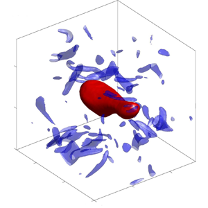
  $t_b$. In figure 2, we show a visualisation of a typical single-drop simulation. Because $d\gg \eta$, breakup is dominated by inertial forces and characterised by the Weber number, ${We} = {\rho \varepsilon ^{2/3} d^{5/3}}/{\sigma }$, and by a characteristic inertial time scale
 \begin{equation} t_d=(d^2/\varepsilon)^{1/3}. \end{equation}
To statistically characterise drop deformation, we perform many independent single-drop simulations initialised with statistically independent turbulent flow fields. Mass leakage (Yue, Zhou & Feng Reference Yue, Zhou and Feng2007) leads to a slow but progressive reduction of the drop diameter and to a time-dependent Weber number,  $We^{\dagger} (t)$, which decreases slightly through the simulations. However, this variation is small and therefore we do not employ any special numerical approach to prevent it (Zhang & Ye Reference Zhang and Ye2017; Soligo, Roccon & Soldati Reference Soligo, Roccon and Soldati2019). We consider the effective Weber number of our simulations as the average Weber number at the average time of breakup, $\langle t_b\rangle$, i.e $We=\langle We^{\dagger} (\langle t_b\rangle )\rangle$. Here the brackets denote the ensemble average. The difference between the time-dependent Weber number at the time of breakup, $We^{\dagger} (t_b)$, and the effective Weber number, $We$, is at most ${\sim }3\,\%$ in the worst cases.

Figure 2. Temporal evolution of a drop at  ${We}=1.8$. The frame is fixed at the centre of the drop and the time of the snapshots corresponds, from left to right, to $t/t_d=2.0$, $2.9$, $4.8$ and $5.1$. Blue isosurfaces denote vorticity with magnitude $|\boldsymbol \omega |=2.6\langle |\boldsymbol \omega |\rangle$, where the brackets denote the ensemble average. The size of the computational box is marked in Kolmogorov units.
We have performed simulations at four different effective  $We\in [1.8,7.4]$. For each $We$, the number of simulations is approximately $100$, which yields a total simulation time of between $300t_d$ and $1500t_d$.
From each simulation, we stored a sufficient number of full flow fields to have fully converged statistics. We analysed flow fields at times at least  $0.5t_d$ after the initial condition and before breakup. We assume that in this time interval the evolution of the drop is statistically stationary. In this range of $We$, breakup occurs in times of the order of the inertial time-scale of the drop, $t_d$. In figure 3(a), we show the median and the standard deviation of the time to breakup, $t_b$, as a function of the $We$. As expected, lower values of the $We$ yield longer times to breakup.

Figure 3. (a) Median time to breakup as a function of the  $We$. The upper and lower bars mark plus-minus the standard deviation. The style of the markers is only used for ease of reference for the data shown in the following panels. (b) Average kinetic energy spectra at $Re_\lambda =58$ for turbulent flow without droplet (dashed line); ${We}=1.8$ (magenta circles); ${We}=5.4$ (blue squares). Vertical dotted lines mark the scale (wavenumber) of the drop, $k_d=2{\rm \pi} /d$, the scale where the spectral density of the kinetic energy dissipation is the highest, $k_\varepsilon$, and the scale of the interface, $k_\delta =2{\rm \pi} /\delta$. The spectra are averaged across the flow fields in the database. (c) Pre-multiplied production spectra, $k\eta \varPhi (k)$. Lines as in panel (b). The total contribution of each wavenumber to the variation of the surface free energy is represented as the area below the curve. Here, $\varPhi$ is normalised with its average in each case.
In what follows, we show that although  $d$ is comparable to the integral scale of the flow, the drop neither modifies the structure of the surrounding turbulence nor resonates with the numerical box. The drop interacts mostly with scales smaller than $d$, which indicates that the linear forcing used to sustain turbulence does not affect breakup. In figure 3(b), we show the average kinetic energy spectrum, $E(k)=2{\rm \pi} k^2 \langle \widehat u \widehat u^* \rangle _k$, with and without an immersed drop. Here $\langle \cdot \rangle _k$ denotes averaging over modes with wavenumber magnitude $k$ and $\cdot ^*$ represents the complex conjugate. The energy spectra are similar for the flow with and without droplet above $k\eta \sim 1$, which suggests a similar turbulent structure at those scales. To further corroborate this, we calculate the skewness and flatness factor of the longitudinal velocity derivatives,
 \begin{equation} \mathcal{F}_n=\frac{\langle (\partial_i u_i)^n \rangle}{\langle (\partial_i u_i )^2\rangle^{n/2}}, \end{equation}
where no summation is intended for repeated indices. We find that, away from the drop surface,  $\mathcal {F}_3\approx -0.52$ and $\mathcal {F}_4\approx 5.2$ independent of the Weber number, which are similar to the values for a simulation without the drop and in the expected range for the $Re_\lambda$ considered (Jiménez et al. Reference Jiménez, Wray, Saffman and Rogallo1993).
The good collapse of the energy spectra at the small wavenumbers (large scales) also suggests the absence of any resonances between the drop and the box, which could lead to spurious large-scale dynamics. To examine how the large-scale forcing affects the dynamics of breakup, we study the pre-multiplied production spectra,  $k\eta \varPhi (k)$, shown in figure 3(c), where
 \begin{equation} \varPhi(k)={-}4{\rm \pi} k^2 \Re\langle\widehat{ \left( u_j\partial_j c\right)}{\widehat \phi}^* \rangle_k, \end{equation}
describes the contribution of each scale to the changes of the surface energy arising from the deformation of the interface by the velocity field. Note that the integral of  $\varPhi (k)$ across wavenumbers is equal to $\langle \vartheta \rangle _S$. Variations of the surface energy arise mostly from turbulent fluctuations at scales below the drop diameter, whereas the contribution of larger scales is comparatively small. In fact, the contribution of the scales affected by the forcing (with $k<2$) to the production of surface energy is slightly negative on average, which confirms that the forcing does not contribute to deformation and breakup.
4. Analysis of the energetic exchange in isotropic turbulence
4.1. Local and non-local surface stretching
Despite the simplicity of the energetic exchange described in § 2, the coupling between the dynamics of the drop surface and the surrounding turbulence is bidirectional and highly nonlinear. The rate-of-strain tensor generates surface contraction or expansion, and, at the same time, the surface dynamics generates straining motions. For instance, as a deformed drop relaxes towards a spherical shape, the surface energy follows damped oscillations before settling into equilibrium (see Appendix A). Although these changes of the surface energy are produced by the stretching and compression of the surface, they are drop induced and not necessarily related to drop breakup.
To separate the dynamics of the interface from the action of the surrounding turbulence, we split the surface-stretching term into contributions related to eddies close to (including those inside) the drop and far from the drop. Here we consider eddies as patches of swirling fluid and associate them with the vorticity field. The kinematic relations that hold between the vorticity vector and the rate-of-strain tensor imply that eddies away from the drop stretch its surface by non-local effects (Ohkitani & Kishiba Reference Ohkitani and Kishiba1995; Hamlington et al. Reference Hamlington, Schumacher and Dahm2008). Let us consider a distance  $\varDelta$, and separate the vorticity field in $\varDelta$-outer and $\varDelta$-inner eddies. The former are defined as eddies a distance $\varDelta$ or further from the drop surface, while the latter correspond to eddies that are closer than $\varDelta$ or inside the drop surface. We define the vorticity field at a distance further than $\varDelta$ from the drop surface as
 \begin{equation} \boldsymbol \omega'^O=G(\boldsymbol x;\varDelta) \boldsymbol \omega, \end{equation}
where  $\boldsymbol \omega =\boldsymbol {\nabla } \times \boldsymbol u$ is the vorticity vector and
 \begin{equation} G(\boldsymbol x;\varDelta)= \begin{cases} 1 & \text{if}\ |\boldsymbol x - \boldsymbol x_s|_s>\varDelta\ \text{and}\ \boldsymbol x \in \mathscr{O}, \\ 0 & \text{if otherwise}, \end{cases} \end{equation}
is a kernel that truncates the vorticity field at a distance  $\varDelta$ from the drop surface. Here $\boldsymbol x_s$ defines the surface of the drop, $|\boldsymbol x - \boldsymbol x_s|_s$ is the shortest Euclidean distance from $\boldsymbol x$ to the drop surface and $\mathscr O$ comprises all the points outside the drop. Let us note that $\boldsymbol \omega '^O$ does not define a vorticity field because it does not locally fulfil $\boldsymbol {\nabla }\boldsymbol {\cdot }\omega ^O=0$, where the truncation is performed. We thus project it into the closest divergence-free field, $\boldsymbol \omega ^O=\boldsymbol \omega '^O - \boldsymbol {\nabla }\psi$, by solving
 \begin{equation} \nabla^2\psi=\boldsymbol{\nabla}\boldsymbol{\cdot}\boldsymbol\omega'^O, \end{equation}
with periodic boundary conditions. We calculate the stretching induced on the drop by the eddies away from its surface from the Biot–Savart law (Ohkitani & Kishiba Reference Ohkitani and Kishiba1995). By taking the curl of the vorticity and considering that  $\boldsymbol {\nabla }\boldsymbol {\cdot }\boldsymbol u^O =0$, we obtain the following equation:
 \begin{equation} \nabla^2\boldsymbol u^O={-}\boldsymbol{\nabla}\times\boldsymbol \omega^O, \end{equation}
which, when solved with periodic boundary conditions, provides the rate-of-strain tensor produced by  $\varDelta$-outer eddies, $S^O_{ij}=\frac {1}{2}(\partial _j u_i^O + \partial _i u_j^O)$, and by $\varDelta$-inner eddies, $S_{ij}^I=S_{ij} - S_{ij}^O$.
The contributions to the stretching of the drop surface by  $\varDelta$-outer and $\varDelta$-inner eddies are
 \begin{equation} \left.\begin{gathered} \vartheta^O={-}\sigma n_iS^O_{ij}n_j,\\ \vartheta^I={-}\sigma n_iS^I_{ij}n_j, \end{gathered}\right\} \end{equation}
respectively, where the rate-of-strain tensor is evaluated at the surface of the drop. A schematic representation of this decomposition and its application to a snapshot of a direct numerical simulation are shown in figure 4(a–c).

Figure 4. (a) Decomposition of the rate-of-strain tensor in contributions arising from eddies a distance  $\varDelta$ from the drop surface, denoted as $S^O_{ij}$, and a distance $\varDelta$ close to the surface (including the inside of the drop), denoted as $S^I_{ij}$. Here $\boldsymbol x_s$ marks the drop surface. Magnitude of the outer (b) and inner (c) rate-of-strain tensor, $2S^O_{ij}S^O_{ij}$ and $2S^I_{ij}S^I_{ij}$, in a direct numerical simulation for $\varDelta =0.19d$ and $We=5.4$. The solid red line marks the drop surface and the dashed magenta line a distance $\varDelta =0.19d$ from the surface. In panel (b), the outer rate-of-strain tensor at a distance smaller than $\varDelta =0.19d$ from the drop surface has been multiplied by $10$ to ease visualisation. Axes in Kolmogorov units.
4.2. Stretching by inner and outer eddies
In this section, we obtain a value of  $\varDelta$ for which the separation in $\varDelta$-inner and $\varDelta$-outer eddies is physically meaningful and practical. We aim to separate the surface stretching into a contribution arising from eddies close to the drop surface, which are affected by surface dynamics or by the material properties of the drop, and another contribution arising from eddies far from the surface, which are independent of surface dynamics or the material properties of the drop.
A practical approach is to find the smallest  $\varDelta$ for which the $\varDelta$-outer eddies and the surface are not coupled, i.e. where the $\varDelta$-outer stretching is independent of surface dynamics. In addition, this approach identifies the smallest region close to the drop surface where eddies are affected by surface dynamics. We denote the $\varDelta$-inner and $\varDelta$-outer eddies identified with this criterion simply as inner and outer eddies.
To find the  $\varDelta$ that separates inner and outer eddies, we use the correlation coefficient between $\vartheta ^O$ with $\vartheta ^I$,
 \begin{equation} \mathcal{C}=\frac{\langle \overline{\vartheta^I}\boldsymbol{\cdot} \overline{\vartheta^O}\rangle}{\sqrt{\langle {\overline{\vartheta^I}}^2\rangle \langle {\overline{\vartheta^O}}^2\rangle}}, \end{equation}
where the bar denotes quantities without their ensemble average,  $\bar {\vartheta }=\vartheta -\langle \vartheta \rangle$. We evaluate $\mathcal {C}$ for different $We$ and $\varDelta$, and show the results in figure 5(a,b). The correlation coefficient is close to unity for $\varDelta$ close to zero, and decays fast with increasing $\varDelta$. For $\varDelta =0.12d$, $\mathcal {C}\approx 0.2$, and for $0.19d$, it drops close to zero. In figure 5(b), we show that the correlation coefficient for $\varDelta =0.12d$ and $\varDelta =0.19d$ is close to zero for all $We$, which indicates that $0.12d<\varDelta <0.19d$ is a reasonable estimate of the distance that separates outer and inner eddies in the range of $We$ considered here. This separation corresponds in Kolmogorov units to $6\eta <\varDelta <9\eta$.

Figure 5. (a,b) Correlation coefficient,  $\mathcal {C}$, between the stretching by inner eddies, $\vartheta ^I$, and outer eddies, $\vartheta ^O$, as a function of $\varDelta$ (a) and $We$ (b).
In the following, we will study the contribution of inner and outer eddies to the surface stretching. For simplicity, we name these contributions as the inner and outer stretching, respectively.
4.3. Statistics of the surface stretching
In figure 6(a–c), we show the probability density function (p.d.f.) of  $\vartheta$, $\vartheta ^O$ and $\vartheta ^I$, measured at the surface of the drop for $We=1.8$ and $5.4$, and $\varDelta =0.12d$. Results are similar for $\varDelta =0.19d$. We find that $\vartheta$ and $\vartheta ^I$ are very similar and display fairly fat-tailed distributions which depend on the $We$. We suggest that these tails are a consequence of surface tension forces produced by the oscillations of the interface. However, the p.d.f.s of $\vartheta ^O$ are more symmetric, closer to a Gaussian. Their good collapse at two different $We$ indicates that the outer stretching is not affected by surface dynamics. These results corroborate that the value of $\varDelta$ used to decompose the flow in inner and outer eddies is adequate.

Figure 6. Probability density function of the local surface stretching arising from the full flow,  $\vartheta$, (a), the inner eddies, $\vartheta ^I$, (b) and the outer eddies, $\vartheta ^O$, (c) for $\varDelta =0.12d$ and at $We=$: solid magenta line, 1.8; dashed blue line, 5.4. Quantities are plotted without the mean and divided by their standard deviation.
In figure 7(a), we show the mean of  $\vartheta$, $\vartheta ^O$ and $\vartheta ^I$ normalised with $\rho u^3_d$, where $u_d=d/t_d$, for different values of $We$. The average of $\vartheta$ increases with $We$, which is consistent with the statistics of the breakup time shown in figure 3(a). We assume that the breakup of an initially spherical drop takes place when a critical increment of the surface energy, $\Delta \mathcal {H}_b$, is reached (Andersson & Andersson Reference Andersson and Andersson2006). Because the surface energy can only increase owing to the stretching term, its average measured on the surface of the drop is related to the time to breakup by
 \begin{equation} t_b\sim\left\langle\frac{\Delta \mathcal{H}_b}{\vartheta d^2}\right\rangle, \end{equation}
which has been estimated by averaging (2.12) in time, considering that the increment of the surface energy is approximately  $\langle \vartheta \rangle d^2$ and neglecting the dissipation of surface energy. The increment of the surface energy required for breakup is approximately the difference between the surface energy after breakup, $\mathcal {H}_b$, and the surface energy of a spherical drop, $\mathcal {H}_0$, i.e. $\Delta \mathcal {H}_b\approx \mathcal {H}_b - \mathcal {H}_0=f\sigma d^2$, where $f\leq f_{b}$ is a factor that depends on the geometry of breakup and is largest for binary breakup, when $f_{b}=2^{1/3} - 1\approx 0.26$ (Andersson & Andersson Reference Andersson and Andersson2006). The time to breakup increases with decreasing $We$, which is consistent with the increment of $\langle \vartheta \rangle$ with $We$.
$We$.

Figure 7. (a) Mean, (b) standard deviation, (c) skewness and (d) excess flatness of  $\vartheta$ as a function of $We$. Mean and standard deviation are normalised by $\rho u_d^3$, where $u_d=d/t_d$. Solid symbols correspond to the statistics of $\vartheta ^O$ and empty symbols to $\vartheta ^I$. Colour lines correspond to $\varDelta =$: solid, $0.12d$; dashed, $0.19d$; and solid black line to the full rate-of-strain tensor. In panel (b), the dotted line is proportional to $We^{-1}$.
The average outer stretching is positive and larger than the inner stretching. It decreases approximately by a factor of  $2$ from $We=1.8$ to $We=7.4$. The inner stretching increases substantially with $We$, transitioning from $\langle \vartheta ^I\rangle <0$ to $\langle \vartheta ^I\rangle >0$ at approximately $We\approx 3.5$. Note that negative average values of the inner stretching indicates that, close to the surface, energy is being mostly transferred from the surface to turbulent fluctuations. This phenomenon will be examined in detail in § 4.5.
In figure 7(b), we show the standard deviation of  $\vartheta$ normalised by $\rho u^3_d$. It is approximately proportional to $We^{-1}$ and substantially higher for the inner than for the outer stretching. In all cases, the standard deviation of the surface stretching is larger than its mean. This is particularly significant for the inner stretching and small $We$, and suggests that a very significant part of the stretching is not efficient and cancels out when averaging.
We focus now on higher-order statistics of the surface stretching, in particular the skewness and the flatness factor, which are defined as
 \begin{equation} F_n(\vartheta)=\frac{\langle(\vartheta-\langle\vartheta\rangle)^n\rangle}{\langle\vartheta^2 -\langle\vartheta\rangle^2\rangle^{n/2}}, \end{equation}
for  $n=3$ and $n=4$, respectively, and are shown in figure 7(c,d). For ease of comparison, we consider the excess flatness factor, which is the flatness factor minus that of a Gaussian distribution, for which $F_4=3$. These statistical moments reflect the strong differences between inner and outer stretching. While the skewness of the outer contributions is close to zero and does not change with $We$, the inner stretching is negatively skewed and its skewness depends on the $We$. The excess flatness factor conveys a similar picture. The outer contributions have a low, $We$-independent, excess flatness factor, whereas for the inner contributions the excess flatness factor increases with decreasing $We$. These results corroborate, first, that the statistics of the outer stretching are $We$-independent, and second, that the inner stretching has an intermittent structure, with intense events of the surface stretching becoming stronger with decreasing $We$. These events are probably related to the relaxation of the drop towards a spherical shape.
4.4. Geometrical characterisation of the inner and outer stretching
To further explain the differences between the inner and outer stretching, and how they change with  $We$, we study the structure of the vorticity vector and the rate-of-strain tensor induced by inner and outer eddies on the surface of the drop. In the spirit of the analysis of vortex stretching in isotropic turbulence (Ashurst et al. Reference Ashurst, Kerstein, Kerr and Gibson1987; Buaria, Bodenschatz & Pumir Reference Buaria, Bodenschatz and Pumir2020), we analyse the surface stretching term in the frame of reference of the eigenvectors of the rate-of-strain tensor and quantify the contribution of each of its eigenvalues to the total surface stretching.
In figure 8(a–c), we show the p.d.f. of the cosine of the angle of alignment between each of the principal axes of the rate-of-strain tensor,  $\boldsymbol v_1$, $\boldsymbol v_2$ and $\boldsymbol v_3$ (where $\lambda _1\le \lambda _2\le \lambda _3$ are their corresponding eigenvalues) and the normal to the surface, $\boldsymbol n$.

Figure 8. (a–c) Probability density function of  $\cos \theta _i=\boldsymbol n \boldsymbol {\cdot }\boldsymbol v_i$, where $\boldsymbol v_i$ are the principal directions of the rate of strain tensor and $\lambda _1\le \lambda _2\le \lambda _3$ are their eigenvalues. Solid markers correspond to angles calculated with $S^{O}_{ij}$ and empty markers to $S^{I}_{ij}$, for $\varDelta =0.19d$. (d) Similar but for the vorticity vector, $\cos \theta _\omega =\boldsymbol n \boldsymbol {\cdot }\boldsymbol \omega /|\boldsymbol \omega |$. Lines correspond to ${We}=$: solid, $1.8$; dashed, $3.6$; dash–dotted, $5.4$. The vertical dotted line in panels (a,c) marks $\cos {\rm \pi}/4$.
For the inner contributions, the most stretching ( $\boldsymbol {v}_3$) and the most compressing ( $\boldsymbol {v}_1$) eigenvectors tend to be oriented at ${\sim }45^{\circ }$ with respect to the surface normal, and therefore also to the surface tangent plane, while the intermediate eigenvalue is predominantly normal to the surface normal (parallel to the surface tangent plane). As shown in figure 8(d), the vorticity vector aligns strongly normal to $\boldsymbol n$ and parallel to the surface. This trend was also reported by Soligo, Roccon & Soldati (Reference Soligo, Roccon and Soldati2020). In all cases, the alignment is more marked for small $We$, which reveals an important effect of surface dynamics on the configuration of the velocity gradients at the surface of the drop.
The stretching of the surface by outer eddies shows a substantially different picture. There is a weak but consistent tendency of the most compressing eigenvector to align normal to the surface tangent plane. The collapse of the p.d.f.s of  $\cos \theta _i$ at different $We$ suggests that this effect is independent of the surface dynamics.
We further decompose the surface stretching term into the contribution from each of its eigenvalues. A possible approach is to consider the rate of compression or stretching of the vector normal to the surface by each eigenvalue,  $r_i=-\sigma \lambda _i\sin \theta _i$ (no summation for repeated indices is intended), which yields
 \begin{equation} \vartheta=r_1 + r_2 + r_3={-}\sigma(\lambda_1\cos^2\theta_1 + \lambda_2\cos^2\theta_2 + \lambda_3\cos^2\theta_3). \end{equation}
However, this decomposition cannot be readily interpreted from a physical perspective. Instead, we consider the contribution of each eigenvalue to the stretching or compression of the surface tangent plane,  $p_i=\sigma \lambda _i\sin ^2\theta _i$. Note that $\sin \theta _i=\cos ({\rm \pi} /2-\theta _i)$ is the projection of each eigenvector on the surface tangent plane. Because $\lambda _1 + \lambda _2 + \lambda _3=0$, and $\cos ^2\theta _i=1-\sin ^2\theta _i$, the total surface stretching reads,
 \begin{equation} \vartheta=p_1 + p_2 + p_3=\sigma(\lambda_1\sin^2\theta_1 + \lambda_2\sin^2\theta_2 + \lambda_3\sin^2\theta_3). \end{equation}
 In figure 9(a,b), we show the averages of  $p_i$ for the inner and outer contributions. In both cases, the surface stretching and compression arising from $p_1$ and $p_3$ is much larger in absolute value than that of $p_2$ (note that in the plot, $p_1$ and $p_3$ are divided by $10$ for ease of visualisation). However, there is a significant cancellation between $p_1$ and $p_3$, and $\langle p_1 + p_3\rangle \sim \langle p_2\rangle$.

Figure 9. (a,b) Average surface stretching owing to each eigenvalue of the rate-of-strain tensor,  $p_i=\sigma \lambda _i\sin ^2\theta _i$, as a function of the Weber number for the inner (a) and the outer (b) contributions, for $\varDelta =0.19d$. The surface stretching is normalised by $\rho u_d^3$. (c) Surface average of the square of the inner rate-of-strain tensor, $2S^I_{ij}S^I_{ij}$, for $\varDelta =0.19d\eta$, and the vorticity vector $\omega _i\omega _i$ for different Weber numbers, normalised with Kolmogorov units. (d) Probability distribution function of $\varLambda =\log _2 |\lambda _1|/\lambda _3$ for different Weber numbers.
For the outer stretching,  $p_1 + p_3$ produce net surface stretching, which stems from the tendency of $\boldsymbol v_3$ to align parallel to the surface (or $\boldsymbol v_1$ normal to it). Conversely, $p_2$ does not contribute on average to the outer stretching. This is in agreement with the almost random orientation of $\boldsymbol v_2$ with respect to the surface normal, as shown in figure 8(b).
For the inner stretching, the cancellation of  $p_1$ and $p_3$ is consistent with a predominant alignment of $\boldsymbol v_1$ and $\boldsymbol v_3$ at ${\sim }45^{\circ }$ with respect to the normal and to the surface tangent plane. In this case, $p_2$ contributes to the average stretching of the surface. As $We$ increases, the absolute value of $\langle p_1 + p_3\rangle$ decreases and $\langle p_2 \rangle$ progressively dominates the average stretching, which leads to $\langle \vartheta ^I\rangle >0$ for $We>3.5$, as shown in figure 7(a).
4.5. Transition from a  $2-D$ to a $3-D$ structure for the inner rate-of-strain tensor


In this section, we explain the transition from  $\langle \vartheta ^I\rangle <0$ to $\langle \vartheta ^I\rangle >0$ at $We\approx 3.5$ by analysing the intensity and structure of the velocity gradients at the drop surface. In figure 9(c), we show the average of $2S^I_{ij}S^I_{ij}$ for $\varDelta =0.19d$ and $\omega _i\omega _i$, measured at the surface of the drop. The intensity of the velocity gradients on the surface of the drop increase with decreasing $We$ owing to surface tension forces, but these forces impose a strong constraint on their structure. This is particularly noticeable in the rate-of-strain tensor, which has a quasi-2-D structure at the low $We$, with $|\lambda _2|\ll |\lambda _3|\approx |\lambda _1|$, and becomes progressively 3-D, $|\lambda _2|\sim |\lambda _3|\sim |\lambda _1|$, as $We$ increases. To characterise this transition, we analyse
 \begin{equation} \varLambda=\log_2 \frac{|\lambda_1|}{\lambda_3}, \end{equation}
at the drop surface. Because  $\frac {1}{2}\lambda _3\leq |\lambda _1|\leq 2\lambda _3$, this quantity is defined in the range $-1\leq \varLambda \leq 1$. Predominant $\varLambda >0$ is characteristic of fully developed 3-D turbulence and implies that $\lambda _2>0$ on average. Conversely, $\varLambda =0$ indicates 2-D dynamics, in which $\lambda _1=-\lambda _3$ and, by continuity, $\lambda _2=-\lambda _1 - \lambda _3=0$. As shown in figure 9(d), the p.d.f. of $\varLambda$ shows that for small $We$,
$We$,  $|\lambda _1|\sim \lambda _3$ and $\lambda _2\ll \lambda _3$. As $We$ increases, the peak of the p.d.f. of $\varLambda$ moves towards $\varLambda \approx 0.4$, which indicates a transition from a quasi-2-D to a 3-D structure of the inner rate-of-strain tensor at the surface. This transition implies that $\lambda _3$ and $|\lambda _1|$ decrease with respect to $\lambda _2$, which leads to $\langle p_2\rangle >\langle p_1 + p_3 \rangle$ and to $\langle \vartheta ^I\rangle >0$.
5. Discussion
We have separated the stretching of the drop surface into contributions from inner and outer eddies, which we have defined in § 4.2. For distances to the drop surface larger than  $\varDelta =0.12d$, the inner and outer stretching are not correlated pointwise (figure 5), which indicates that beyond this distance, the outer stretching is independent of surface dynamics. This is corroborated by the statistics of the outer surface stretching for this $\varDelta$, which are roughly $We$-independent. We have shown that the outer stretching is dominant and contributes on average to the increment of the surface energy at all $We$.
$We$.
Conversely, the average of the inner stretching is negative for  $We<3.5$, which indicates a predominant flux of energy from the surface into turbulent fluctuations. We interpret this flux of energy as the generation of inner eddies arising from the relaxation of the surface. Above $We\approx 3.5$, the average inner stretching becomes positive, which indicates that, on average, also inner eddies contribute to drop deformation. In all cases, the inner stretching shows non-Gaussian and negatively-skewed $We$-dependent statistics. Negative events of the inner stretching become more intense as $We$ decreases, which evidences the action of the surface to restore deformations by transferring the surface energy back to turbulent fluctuations.
At low  $We$, the net increments of the total surface energy depend on the interplay between the outer surface stretching, which constitutes a mechanism of net drop deformation, and the ability of the surface to restore this deformation by transferring energy to inner eddies, which provide a source of energy dissipation through molecular viscosity. In addition, we have shown that at low $We$, the rate-of-strain tensor is constrained by surface tension forces. Although its average magnitude is larger than in the turbulent background, which provides enhanced dissipation of turbulent kinetic energy, its 2-D structure and its configuration with respect to the interface precludes the net stretching of the surface. As $We$ increases, the inner rate-of-strain tensor develops a 3-D structure in which its intermediate eigenvalue becomes predominantly positive, which produces net stretching of the surface. This phenomenon explains the transition at $We\approx 3.5$ from a net energy transfer from the surface to inner eddies (negative inner stretching), to a net energy transfer from inner eddies to the surface (positive inner stretching).
We have reported a statistically significant alignment of the surface normal vector with the most compressing direction of the rate-of-strain tensor induced by outer eddies and of the surface tangent plane with the most stretching one. This phenomenon, which is also observed in the evolution of passive material surfaces in turbulence and naturally leads to these alignments (Girimaji & Pope Reference Girimaji and Pope1990), indicates the persistent stretching of the drop surface by outer eddies. The alignment statistics are similar at different  $We$, which corroborates that this mechanism is independent of surface dynamics.
6. Conclusions
In this work, we have analysed the energetics of fluid–fluid interfaces. One of our main contributions is to provide a mathematical description of the mechanism responsible for the exchange between the kinetic energy of the flow and the surface energy of the fluid–fluid interface. We have shown that this exchange occurs owing to the stretching or compression of the surface area by the rate-of-strain tensor (see (2.15)–(2.17)), in a mechanism analogous to the stretching of the vorticity field in turbulence. This analytical result highlights the relevant role of straining motions in drop deformation and breakup, in agreement with experiments and theoretical analyses of laminar flows in the Stokes limit (Rallison Reference Rallison1984).
In the context of drop deformation and breakup, this mathematical analysis provides a solid framework to quantify the energetic exchanges between the surface and the kinetic energy fluctuations of the surrounding turbulence. By leveraging the non-local nature of turbulence, we have separated the total stretching into contributions from inner and outer eddies. We use here the term outer to refer to eddies sufficiently far from the drop surface for their dynamics to be unaffected by surface tension forces. Conversely, we define inner eddies as those close to the surface or inside the drop, whose dynamics are affected either by surface tension forces or by the material properties of the fluid inside the drop. We have shown that the stretching of the drop surface by outer eddies contributes substantially to the deformation of the drop and is relevant to drop breakup. This mechanism constitutes a physically well-defined, quantitative reinterpretation of the phenomenological ‘collision’ of eddies (Luo & Svendsen Reference Luo and Svendsen1996).
Our results justify a ‘stochastic’ approach to breakup modelling, particularly at low  $We$. Outer eddies provide the main source of drop deformation. They are not locally coupled to inner eddies or to the dynamics of the interface, which precludes synergies between inner and outer eddies that may lead to enhanced breakup (at least in the case of similar density and viscosity investigated here). For sufficiently long breakup times, the stretching by outer eddies may be modelled as a stochastic forcing with statistical properties that depend mostly on the surrounding turbulence. Although the surface stretching by inner and outer eddies is not coupled locally, it is likely globally coupled, for instance, owing to energy conservation.
Our results suggest that for low  $We$ ( $We<3.5$), drop deformation and breakup occur as an interplay between inner and outer dynamics, where the latter is the driver and a source of surface energy increments, while the former is a sink. The stretching by outer eddies is mostly balanced by an energy transfer from the surface to inner eddies, which provide a source of dissipation and prevents the buildup of surface energy.
Although our study is limited to the ideal case of incompressible fluids with equal density and viscosity, the theoretical analysis in § 4 applies equally to compressible fluids, and to fluid pairs with different viscosity and density. For instance, we suggest that an increment of the drop viscosity affects the inner eddies owing to, first, the kinematic relations imposed on the rate-of-strain tensor across the interface, which depend on the viscosity ratio (Dopazo et al. Reference Dopazo, Lozano and Barreras2000), and second, the enhanced ability of the fluid inside the drop to diffuse momentum and dissipate energy. These changes may inhibit the stretching of the surface by inner eddies and/or provide a fast mechanism to dissipate the surface energy produced by the stretching of outer eddies, which explains the resistance of viscous drops to breakup (Calabrese, Chang & Dang Reference Calabrese, Chang and Dang1986; Roccon et al. Reference Roccon, De Paoli, Zonta and Soldati2017). Our analysis also applies to bubbles. We suggest that our decomposition allows a separation of the effect of the bubble's natural oscillations from that of turbulence, which enables an exploration of how resonances with the characteristic oscillatory frequency affect breakup (Risso & Fabre Reference Risso and Fabre1998).
An important question that we have not addressed in this work is whether breakup occurs as a progressive buildup of surface energy arising from the accumulative interaction with many eddies or as sharp increments of the surface energy owing to interactions with isolated intense turbulent events. Although answering this question necessarily requires temporal analysis, we have shown that the standard deviation of the local surface stretching is much larger than its mean, possibly reflecting inefficient stretching that cancels out. Moreover, at low  $We$, the stretching by outer eddies is mostly balanced by a transfer of energy back to turbulent fluctuations (inner eddies), which precludes the buildup of surface energy. These results suggest that the weak turbulent background produces much of this ineffective stretching, whereas the interaction of the drop with just a few intense turbulent structures produces the effective stretching leading to breakup.
Acknowledgement
We thank M.P. Encinar for fruitful discussions and comments on the content of the manuscript.
Funding
A.V.-M. acknowledges the support of the European Research Council COTURB project ERC-2014.AdG-669505.
Declaration of interests
The authors report no conflict of interest.
Appendix A. Code validations: oscillations of a viscous drop in a quiescent fluid
We validate the Cahn–Hilliard–Navier–Stokes code by simulating the oscillations towards equilibrium of a drop in a quiescent fluid. We introduce a drop in a flow without velocity fluctuations and deform it slightly with an axisymmetric perturbation, so that its evolution towards equilibrium is linear and can be described in terms of axisymmetric spherical harmonics. The solution of this flow was given by Lamb (Reference Lamb1924), and reads
 \begin{equation} r(\theta,t)=r_0 + \epsilon P_n(\cos\theta)\cos(f_n t)\exp(-\gamma_n t), \end{equation}
where  $r_0=d/2$ is the radius of the spherical drop, $\epsilon \ll r_0$ is the perturbation magnitude and $P_n$ is the Legendre polynomial of order $n$. Here $f_n$ and $\gamma _n$ are the characteristic oscillation frequency and decay rate of each harmonic,
 \begin{equation} f^2_n=\frac{\sigma}{\rho d^3}\frac{n(n-1)(n+1)(n+2)}{2n+1}, \end{equation}
and
 \begin{equation} \gamma_n=\frac{\nu}{d^2}\left(n(n-1) + (n+1)(n+2)\right), \end{equation}
respectively. Here  $\sigma$ is the surface tension, and $\rho$ and $\nu$ are the density and the kinematic viscosity of the fluid, respectively. The two characteristic time scales of the problem are $\sqrt {\rho d^3/\sigma }$ and $d^2/\nu$. Their ratio, the Ohnesorge number, ${Oh}=\sqrt {\rho /(\sigma d)}\nu$, is the only parameter of the problem.
We consider a spherical drop with  ${Oh}=0.013$ and perturb only its second harmonic, $n=2$. We measure the oscillation of the interface in the direction of the longest semiaxis of the drop ( $\theta =0$ and $P_2=1$), and compare it with the analytical solution. The numerical parameters of the code are the same as those used in the single-drop simulations. In figure 10, we show the evolution of
 \begin{equation} {\Delta r}={r(0,t) - r_0}, \end{equation}
in the simulation and the analytical solution,
 \begin{equation} {\Delta r}=\epsilon\cos(f_n t)\exp(-\gamma_n t). \end{equation}
The match between the two is very good. The characteristic oscillatory frequency given by the code matches the analytical solution with less than  $1\,\%$ error, whereas the decay rate is reproduced with less than $4\,\%$ error.

Figure 10. Comparison of the analytical solution of  $\Delta r/\epsilon$ for a drop with ${Oh}=0.013$ with a numerical simulation with a Cahn–Hilliard–Navier–Stokes (CHNS) code.


 Open access