Introduction

Climate models synthesize current understanding of complex interactions of various elements of the global climate system that may be important to evolution, particularly in terms of the atmosphere, oceans, cryosphere and biosphere. Observational data provide much information on current or past climatic conditions, but do not provide a clear picture of the future climatic evolution, because extrapolation to the future based on past conditions is unreliable when a highly nonlinear system is used. Models therefore constitute the only predictive tool available for investigating future climate change, for example under conditions of enhanced greenhouse-gas forcing.

Abstract theories and models need to be validated in order to develop an acceptable degree of confidence in their projections and analyses. Often, however, the geographical distribution of observational data is highly heterogeneous, even over continental areas where mosi of the data is to be found. There is a lack of direct climatological information over oceanic regions (although satellite remote sensing has been filling this gap in recent years), regions of complex orography and polar regions.

Cryospheric data can be used as a proxy for temperature and precipitation, particularly in remote mountain regions or boreal zones where instrumental climate records are non-existant. The quantity and quality of information on the equilibrium-line altitude (ELA) of glaciers on the one hand, and the evolution of permafrost on the other hand, are good indicators of climate variability on scales ranging from years to centuries; these types of record are dependent on temperature and precipitation, both seasonal and annual, and cumulative over longer periods (i.e. they represent the “memory” of past climatic conditions).

Few, if any, climate-modeling studies have used cryo-spheric records for intereomparison purposes. This paper will discuss briefly the current status of climate models and the type of corresponding cryospheric data that could be used for model intereomparison purposes.

Climate Models: Applications to Polar and High Mountain Regions

High-resolution climate modeling has opened up new perspectives for understanding some of the mechanisms behind climate change. High resolution is obtained either through reducing the grid size of general circulation models (GCMs), or coupling detailed limited-area models (LAMs) to GCMs over a particular region of interest. Combining both techniques allows a very high resolution to be obtained (e.g. Reference Beniston, Ohmura, Rotach, Tschuck, Wild and MarinucciBeniston and others, 1995; Reference Marinucci, Giorgi, Beniston, Wild, Tschuck and BernasconiMarinucci and others, 1995; Reference Rotach, Wild, Tschuck, Beniston and MarinucciRotach and others, in press).

There are about 30 GCMs that have been developed worldwide for climate research. Many of these have been used by the Intergovernmental Panel on Climate Change (Reference Houghton, Jenkins and EphraumsHoughton and others, 1990, Reference Houghton, Callander and Varney1992, Reference Houghton, Meiro Filho, Callander, Harris, Kattenburg and Maskell1996) for assessing model capability in reproducing present-day climate, and for providing an insight into the future, greenhouse-gas enhanced climate of the 21st century. In terms of current climate simulations, current models now capture many elements of the observed climate with a reasonable degree of accuracy, even on a continental scale, particularly when initialized with observed sea-surface temperature distribution and its recent evolution.

Experiments with the European Centre/HAMburg (ECHAM) GCM for conditions of doubled atmospheric concentrations of CO₂ are illustrated in Figure 1 (Reference Beniston, Ohmura, Rotach, Tschuck, Wild and MarinucciBeniston and others, 1995). The global mean temperature increase in this experiment, with respect to the current climate simulation, is 1.5°C. This indicates that the predicted increase in temperature over different regions is largest over continents and at high latitudes. The land surface is responding faster to greenhouse forcing than is the ocean, due to the large thermal inertia of the latter. The retreating snow cover and sea ice, and associated positive feedbacks, lead to the amplification of greenhouse forcing at higher latitudes. The increase in air temperature in the Arctic is strongest during autumn, which can he explained by delayed sea-ice formation in fall.

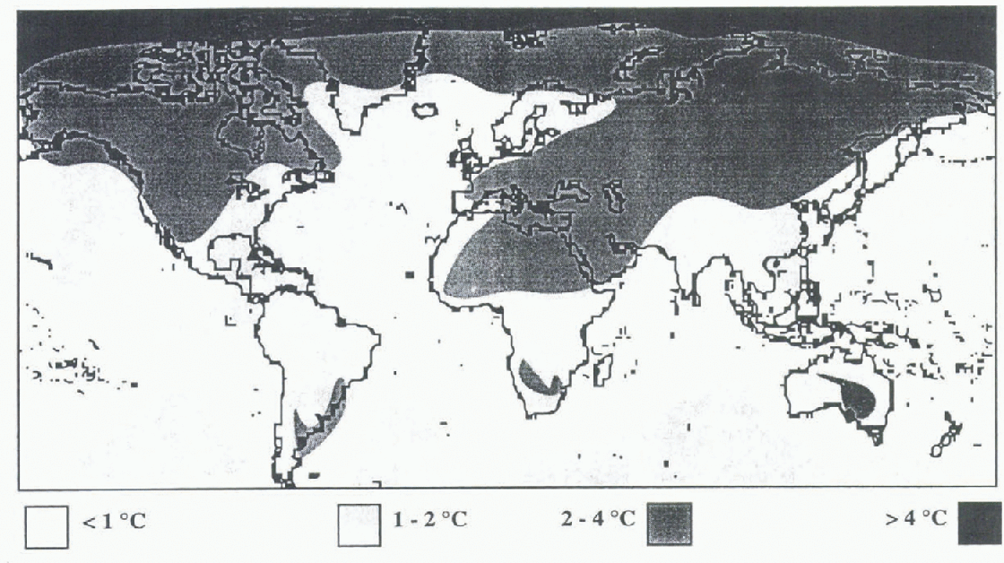
Fig. 1. Changes in annual mean global temperatures between current climate and 2 × CO² climate as simulated by the ECHAM GCM of the Max-Planck Institute for Meteorology.

The regional detail in the global mean temperature increase of 1.5°C is, in a large extent, absent. In high latitudes and in regions of complex orography, certain climatological features that may be significant on a regional scale are not resolved even by the relatively dense grid network of the ECHAM GCM. One method of overcoming this problem is to couple, or “nest” a LAM within the GCM grid structure in order to enhance regional climatological detail.

A coupled GCM-LAM approach has been applied in the Alpine region at a very high spatial resolution by Reference Beniston, Ohmura, Rotach, Tschuck, Wild and MarinucciBeniston and others (1995), specific aspects of which are reported by Reference Marinucci, Giorgi, Beniston, Wild, Tschuck and BernasconiMarinucci and others (1995) and Reference Rotach, Wild, Tschuck, Beniston and MarinucciRotach and others (in press). The ECHAM GCM at T-106 spectral resolution has been used to provide initial and boundary conditions to the Regional Climate Model Version 2 (RegCM2) LAM, developed at the National Center for Atmospheric Research (US) (NCAR). The LAM has a resolution of 20 km, which allows a much better definition of Alpine orography than the 120 km of the driving GCM. An example of the average January and July precipitation patterns over the Alps in a wanner global climate (the CO² doubling experiment) is illustrated in Figure 2. The structure of the precipitation fields reflects, to a large extent, the presence of the orography, as would be expected from the enhanced Spatial definition of the LAM gridmesh. Temperature patterns also reflect the detail of the underlying surface, thereby emphasizing the need for higher spatial resolution in order to investigate climate and climate change over a particular region, especially if that region has complex topography.

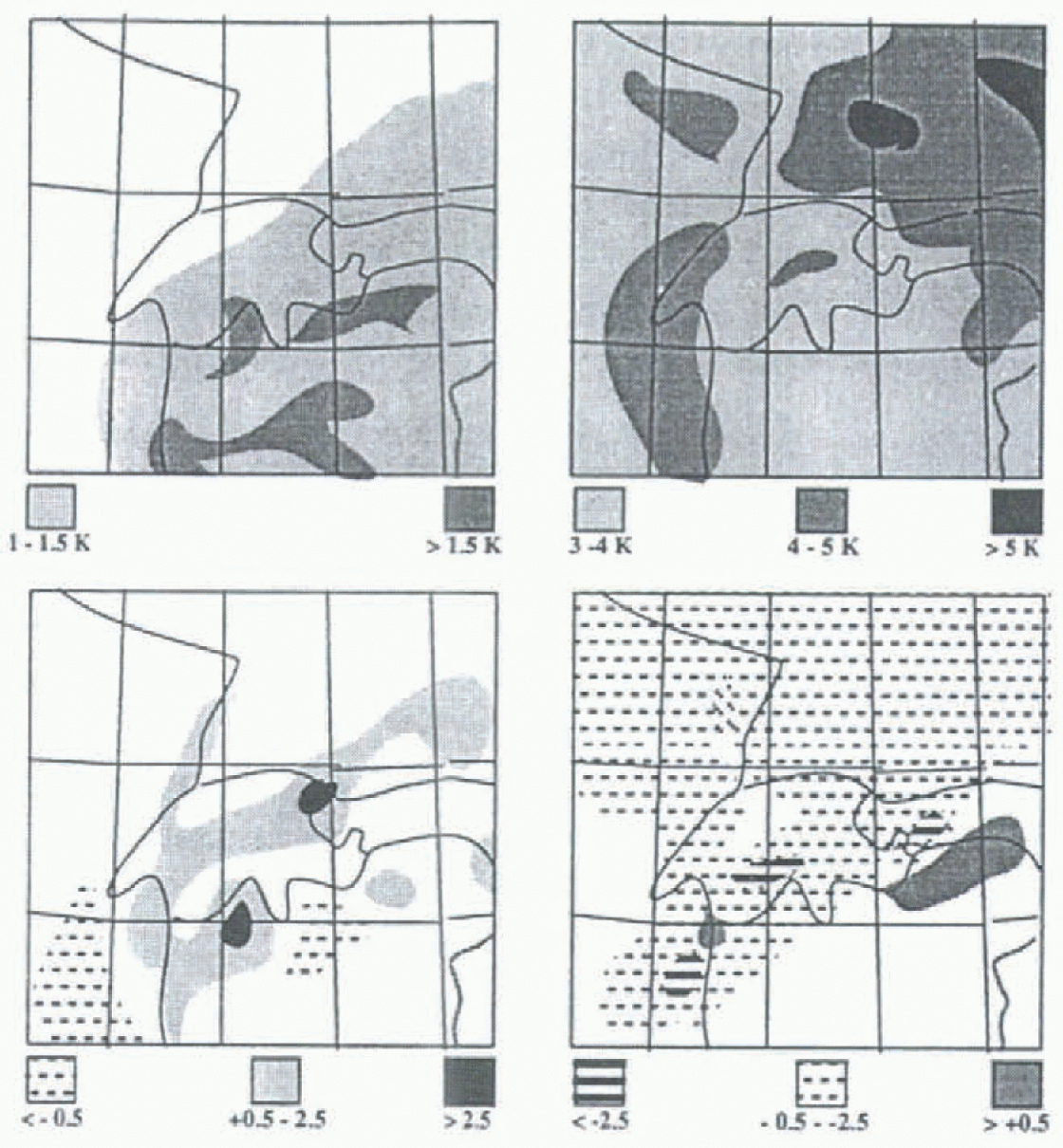
Fig. 2. Upper: LAM-simulated temperature changes in January (left) and July (right), between current and 2 × CO₂ climate in °K; Lower: as for upper, except for precipitation changes in mm d¹.

High-resolution simulations, such as those illustrated here, have contributed to a further improvement of our understanding of the underlying mechanisms of climate change, and have helped point out model deficiencies. Some of these deficiencies are linked to a lack of observational data that could help improve model performance in remote zones, such as in high latitudes or areas of complex orography. In these regions, certain forms of proxy data might be used to reconstruct climate and its recent Huclualions. Direct intercomparison with model results is complex because of the problems associated with the spatial and temporal resolution of the models, which may not correspond to the spatial distribution of the observations (e.g. for mountain glaciers), and because of incomplete physical parameterizations, which may not be simulating the complete physics associated with, for example, permafrost and active layer thickness.

However, some of the very high-resolution model simulations discussed here go some way in alleviating these problems. Solutions can be found on a case-by-case basis for models of different scales (from the global GCMs to the high-resolution LAMs). For example, analyses of ELA data for different mountain regions of the world might provide a detailed picture of zonal and meridional temperature/precipitation gradients at high elevations that are not available from the meteorological instrument record. Model performances, particularly LAMs, in reproducing the observed gradients could thereby be assessed and, wherever necessary, parameterizations improved. In the case of permafrost in boreal zones, observations might help determine the discrepancies between surface sensible and latent heat fluxes in the models. Most Climate models project much larger temperature and precipitation changes in northern latitudes than the global average, because of the high sensitivity of the surface energy budget to shifts in snow cover and corresponding ground temperatures. Under these circumstances, verifying the model performance through proxy permafrost borehole observations becomes crucial.

Because of projected improvements in climate models in coming years, the use of cryospheric data will become increasingly important for verification purposes, since it is anticipated that problems relating to model resolution and physics will be reduced. The following sections will introduce the existing data from high latitudes and mountainous regions that could be used for climate model intereomparison purposes.

Glaciers

Worldwide collection of standardized observations on changes in mass, volume, area and length of glaciers with time (glacier fluctuations), as well as statistical information on the distribution and characteristics of perennial surface ice in space (glacier inventories) is coordinated by the World Glacier Monitoring Service (WGMS) under the auspices of the International Commission on Snow and Ice (ICSI) (Reference Haeberli, Bösch, Scherler, Østrem and WallénHaeberli and others, 1989; Reference Haeberli and HoelzleHaeberli and Hoelzle, 1993; Reference Haeberli, Hoelzle and BöschHaeberli and others, 1994). Data are periodically published (for instance Reference Haeberli, Bösch, Scherler, Østrem and WallénHaeberli and others, 1989; Reference Haeberli and HoelzleHaeberli and Hoelzle, 1993; Reference Haeberli, Hoelzle and BöschHaeberli and others, 1994; cf. also Reference Haeberli and WallénHaeberli and Wallén, 1992; Reference HaeberliHaeberli, 1995) and are incorporated in the World Data Center for Glaciology (WDC-A) and the Global Resources Information Database (GRID) of the Global Environment Monitoring System (GEMS/UNEP).

An extensive database on topographic glacier parameters is being developed in the context of regional glacier inventories. World glacier inventory: status 1988 is a guide to the existing statistical database on the worldwide distribution, and contains information on the morphological characteristics of glaciers as documented in regional inventories (some of which are detailed, while others are preliminary; Reference Haeberli, Bösch, Scherler, Østrem and WallénHaeberli and others, 1989, Reference Haeberli, Hoelzle, Keller, Schmid, vonder Mühll and Wagner1993, Reference Haeberli, Hoelzle and Bösch1994). Repetition of such glacier-inventory work is planned at time intervals that are comparable to the characteristic dynamic response times of mountain glaciers (i.e. a few decades). This should help with analyzing changes on a regional scale, and with assessing the representativity of continuous measurements that can only be carried out on selected glaciers. In addition, glacier-inventory data also serve as a statistical basis for extrapolating the results of observations or model calculations concerning individual glaciers (Reference OerlemansOerlemans, 1993a), and to simulate regional aspects of the effects of past and potential future climate change.

This latter application requires the introduction of a parameterization scheme using the four main geometric parameters contained in detailed inventories (length; maximum and minimum altitude along the central flowline; and surface area) and using correspondingly simple algorithms for deriving such parameters as overall slope, mean and maximum thickness, ELA, mass balance at the glacier terminus, response time, etc. A test study in the European Alps (Reference Haeberli and HoelzleHaeberli and Hoelzle, 1995) indicates a total Alpine glacier volume of some 130 km³ in the mid-1970s. Total loss in Alpine surface-ice mass from 1850 to the mid-1970s is estimated at about half the original value. An acceleration of lhis situation, with annual mass losses of around 1ma⁻¹ or more, as anticipated from IPCC scenario A for the coming century, would lead to the disappearance of a major part of current Alpine ice within decades. The striking sensitivity of glaeierization in cold, mountainous areas, wiih respect to trends in atmospheric warming is clearly observed.

An important parameter for the potential application of glacier inventory information to GCM validation is mean glacier elevation, as contained in detailed glacier inventories (Fig. 3). This easily determined parameter is a rough approximation to ELA. As such, it is associated with continentality and, hence, with annual precipitation, mass balance gradient (activity index), mass turnover, englacial temperature and glacier/permafrost relations (Reference KuhnKuhn, 1981; Reference HaeberliHaeberli, 1983; Reference Oerlemans and PeltierOerlemans, 1993b). Information on mean glacier elevation is of paramount importance for glaciological modeling and hydrological assessments (e.g., Reference Kotlyakov and KrenkeKotlyakov and Krenke, 1982; Reference Haeberli and HoelzleHaeberli and Hoelzle, 1995).

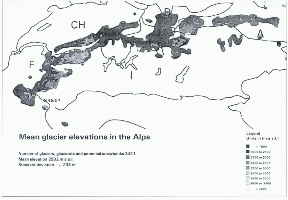
Fig. 3. Mean glacier elevation in the European Alps as based on glacier inventories compiled for Austria (1969), France (1967–71), Germany (1979), Italy (1975–84) and Switzerland (1973).

With respect to glacier fluctuations, annual glacier mass balances are being measured on about 50 glaciers, mainly in the Northern Hemisphere, whereas length changes on about 1000 glaciers will help to assess the global long-term representativity of the limited number of mass balance measurements. An assumed step change in ELA induces an immediate step change in specific mass balance. The resulting change in specific mass balance is the product of the shift in ELA and the gradient of mass balance with altitude, weighted by the distribution of glacier surface area with altitude (hypsometry). Hypsometry represents the local/individual or topographic aspect of glacier sensitivity, whereas the mass balance gradient reflects principally the regional or climatic aspect (Reference KuhnKuhn, 1990). As the mass balance gradient tends to increase with increasing humidity (Reference KuhnKuhn, 1981), the sensitivity of glacier mass balance with respect to changes in ELA is generally much higher in areas with humid/maritime than dry/continental climatic conditions (Reference Oerlemans and PeltierOerlemans, 1993b).

Results from continuous mass balance observations during the period 1980–93 in North America, Eurasia and Africa are summarized in Figure 4. The mean of all 33 glaciers is strongly influenced by the great number of Alpine and Scandinavian glaciers. A mean value was therefore also calculated using only a single (in some places averaged) value for eleven of the mountain ranges involved. Fhc annual signal of the mean mass balance is smaller than the regional variability, but can be improved by cumulating mass balance values over extended periods of time. The mean specific net balance (−0.3 m w.e.) over the entire period reflects an additional energy flux of 3 W m² — chararteristic energy fluxes involved with the shrinkage of mountain glaciers roughly correspond to the estimated radiative forcing. Decadal to secular trends appear to be comparable beyond the scale of individual mountain ranges, with continentality of the climate being the main classifying factor (Reference Letréguilly and ReynandLetréguilly and Reyuaud, 1990) along with individual hypsometric effects (Reference Furbish and AndrewsFurbish and Andrews, 1984; Reference Tangborn, Fountain and SikoniaTangborn and others, 1990). However, detailed analyses reveal considerable spatio-temporal variability over short time periods. Results from worldwide glacier mass-balance programs thus constitute an important key factor in validating time-dependent climate models on both global and regional scales. Algorithms for relating atmospheric temperature and precipitation to ELA, for potential application in GCMs and LAMs, have been developed by a number of authors (e.g. Reference Kuhn and OerlenmansKuhn, 1989; Reference OerlemansOerlemans, 1993a, Reference Oerlemans and Peltierb).

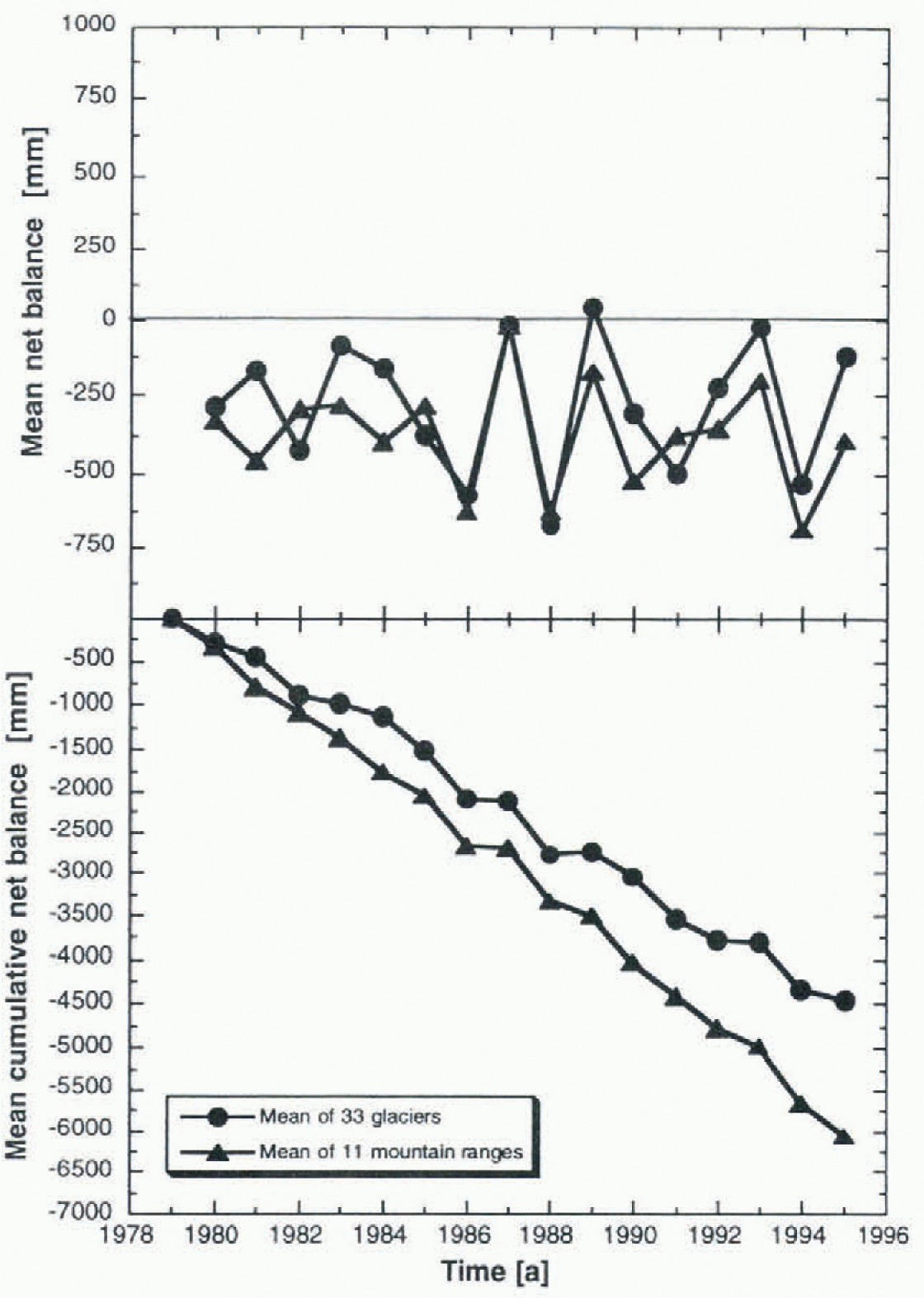
Fig. 4. Mean net balance (upper) and cumulative-mean net balance (lower) continuously measured for the period 1980–93 on 33 glaciers in 11 mountain unices (from Reference Haeberli, Hoelzle and BöschHaeberli and others, 1994).

At the sub-zero temperatures that predominate at high latitudes, regions of continental climate and high altitudes, atmospheric warming in firn does not lead directly to mass loss through melting and/or runoff but rather to the warm-ing of layers, thereby producing corresponding signals in firn/iee temperature profiles with depth (Reference BlatterBlatter, 1987; Reference Haeberli and FunkHaeberli and Funk, 1991; Reference RobinRobin, 1983). For periods corresponding to dynamic-response time, or to multiples of it, cumulative glacier-length changes can be interpreted in terms of the av erage mass balance during the time interval under consideration. In the European Alps, for instance, such analyses confirm the representativeness of the few secular glacier mass balances that have been determined by repeated precision mapping (Reference Haeberli and HoelzleHaeberli and Hoelzle, 1995). The cumulative length change of glaciers constitutes the basis of global intereomparison of secular mass losses.

Permafrost

Some 25% of the Earth’s land surface is permafrost, highlighting the importance of the circumpolar regions as both a boundary condition for GCMs, and a locale where verification should be achieved. Permafrost is a direct physical consequence of severe past and present climates and, as such, provides unique opportunities to study the interactions between die ground and die overlying atmosphere, and the impact of future climate warming on a sizeable part of the Earth. The long-term response of frozen ground to climate change will the controlled by the large reservoir of latent heat. The Global Change Working Group of the International Permafrost Association (IPA) has canvassed researchers around the world who are monitoring changes in permafrost. Sites with measurements dating back several decades, transects crossing the discontinuous to continuous permafrost transition, and intensely instrumented sites stdying near-surface heat-transport processes have been identified, and may contribute to the goals outlined above.

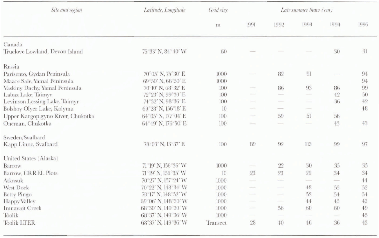
Decadal changes to the thickness of the active layer overlying permafrost will be a sensitive indicator of any climate change, and the vegetation modification that may accompany it. The Circumpolar Active Layer Monitoring Program (CALM) has developed a statistically robust strategy for long-term measurement of the active layer by simple probing on a standard grid (personal communication with Nelson and others, 1995). CALM has been adopted for the International Tundra Experiment sites (ITFX) and die GTOS of WMO/UNESCO/UNEP/ICSU (1995) at independent sites (Table 1). Some researchers are installing frost tubes to record the maximum development of the active layer each season (Reference Nixon, Taylor, Allen and WrightNixon and others, 1995) while new approaches are being used to map soil moisture content from satellite imagery (Reference Kane, Hinzman, Yu and GoeringKane and others, 1994). This is an important parameter for models, while other instrumentation improves our understanding of the mechanisms of heat transfer within the active layer (e.g. Reference Hinkel and OutcaltHinkel and Outcalt, 1995).

Table 1. Circumpolar active layer monitoring (CALM) Program. Note: abstracts and posters reporting these results were presented and published in April 1996 at the ITEX workshop in Copenhagen and the geocryology conference in Pushchino. Additional mountain site and those measuring soild temperatures are being identified and will be added to the network and reported with 1996 observations (Reference BnownBrown, 1996, Reference Brown and Crawford1997)

From a different perspective, currently available maps of surficial geology, soils, vegetation and present climate parameters, and the physics of heat transfer have been used in a geographic information system (GIS) to predict permafrost occurrence and thickness over areas of thousands of square kilometres in the discontinuous permafrost zone. These maps can also be used to predict the impact of climate warming on critical areas of marginal permafrost (Reference Wright, Smith and TaylorWright and others, 1994). Reference Hoelzle and HaeberliHoelzle and Haeberli (1995) outline similar approaches with mountain permafrost. Such a model. embodying surface properties and dynamics known today, might represent the ground surface-boundary condition in future GCMs (or perhaps in higher-resolution LAMs) by refining the surface sensible and latent heat fluxes. Such a map-based model allows an estimation of the rate of release of greenhouse gases, particularly methane, from the huge store of carbon in the tundra, presently also being measured at many sites (Reference Kvenvoldon and LorensonKvenvolden and Lorenson, 1993).

Observational networks are being maintained to ensure that long-term time-series of data will be available in the future that will allow the detection of subtle changes. Watershed ecology (Reference Thorsteinsson and TaylorThorsteinson and Taylor, 1994), permafrost forms and geomorphology (personal communication with E. Kolstrup, 1995), and particularly changes with elevation (Reference Corte and SennesetCorte, 1988; Reference Haeberli, Hoelzle, Keller, Schmid, vonder Mühll and WagnerHaeberli and Others, 1993), are also being monitored. The working group on mountain permafrost within the IPA is presently undertaking attempts to build up a long-term monitoring programme (Fig. 5) as well as a mapping programme on a number of different scales.

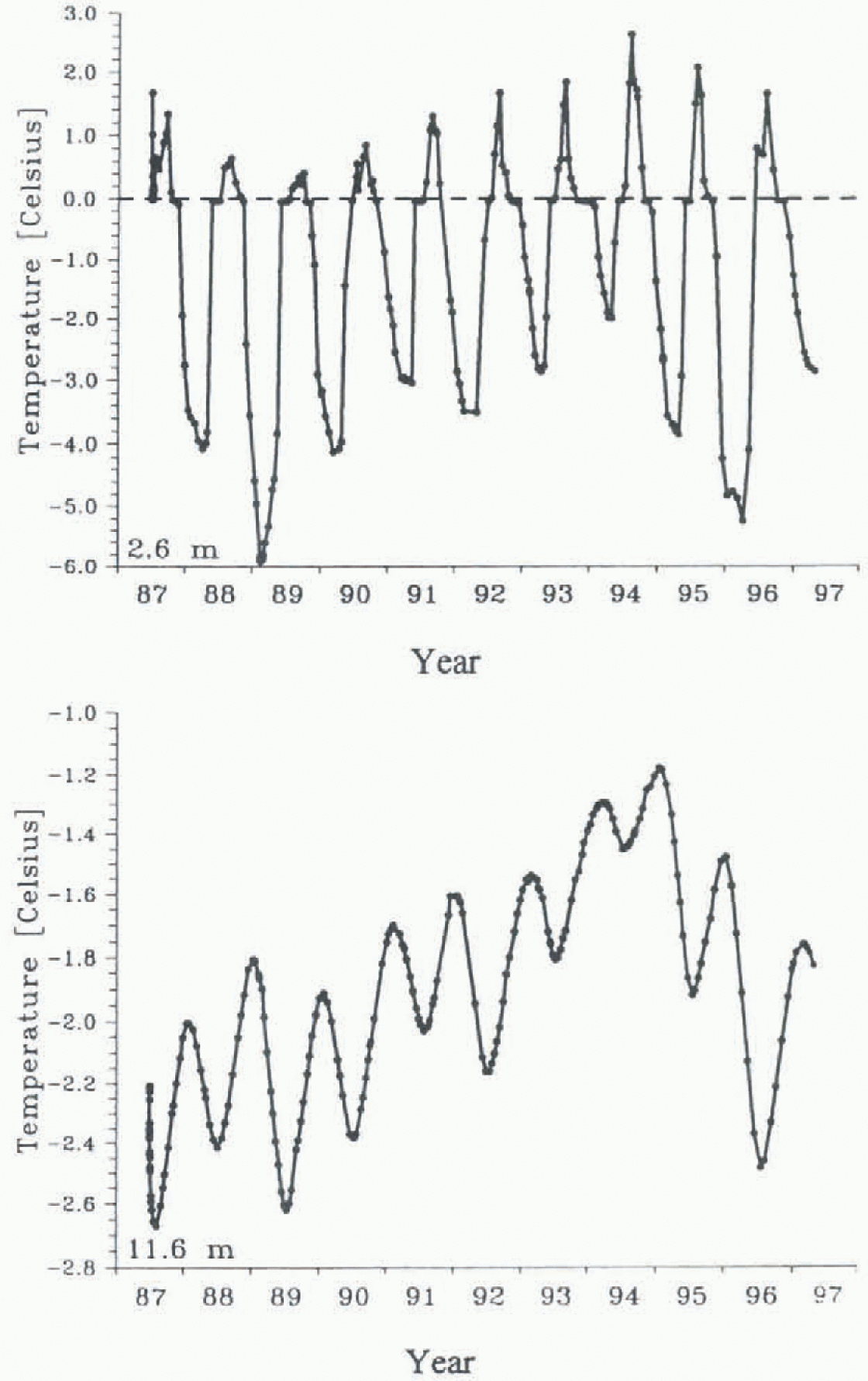
Fig. 5. Temperature evolution at 2.5 m depth (active layer) and at 11.5m Within the permafrost borehole Murtèl/Corvatsch (eastern Swiss Alps). Active-layer temperatures help with understanding energy-exchange processes at the surface and can be used for calibrating statistical relations between ground temperatures and meteorological parameters (such as air temperature and precipitation). Heat-conduction effects filter out high-frequency irregularities at the surface and show longer-term trends with extreme clarity. Snow-poor winters in 1988–89, 1994–95 and 1995–90 with intense ground cooling interrupt the general-warming trend since the late 1980s.