1.1 Basic considerations

In the initial stages of the discussion of the CO₂-climate problem the CO₂-induced global warming was computed by means of climate models based on the assumption of radiative equilibrium between incoming and outgoing radiation fluxes on Earth. Recently attention has been called to the fact that the world ocean has a considerable heat capacity, and that the radiation budget is not balanced while the ocean is being heated up (Reference Thompson and SchneiderThompson and Schneider 1979, Reference Hoffert, Callegari and HsiehHoffert and others 1980, Reference Cess and GoldenbergCess and Goldenberg 1981, Reference HansenHansen and others 1981). We present here results of simulations of the delay and attenuation of the C0₂-induced temperature change by the oceanic heat uptake, obtained using the box-diffusion model (Reference Oeschger, Siegenthaler, Schotterer and GugelmannOeschger and others 1975) with an eddy diffusion coefficient K = 7 685 m² a⁻¹ (2.4 cm² s⁻¹). This value has been obtained from a re-calibration of the box-diffusion model using bomb-produced ^l4C (Reference SiegenthalerSiegenthaler 1983) and is larger than the value obtained using the natural ¹⁴C distribution for. calibration (4 000 m² a^−l). Our results are partly similar to others, although obtained independently. The general discussion will therefore be relatively short. For further details, reference is made to the cited literature, especially to Reference Hoffert, Callegari and HsiehHoffert and others (1980) who used a model similar to the box-diffusion model for simulating oceanic heat transport, and who dwelt on several aspects of the problem.

Changes of the global mean surface temperature T are considered first. A global energy balance for the Earth (per m² of Earth surface) can be written as

(1)

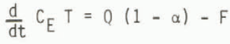
The left-hand term symbolizes changes in global heat storage with C_E representing the effective heat capacity of the Earth; it will be discussed in paragraph 1.3. On the right are the radiation fluxes at the boundary of the Earth-climate system, i.e. at the top of the atmosphere. Q is the incident solar radiation, assumed constant, α is the global albedo and F denotes the outgoing infrared flux at the top of the atmosphere.

1.2 Heat flux parameterization and equilibrium temperature changes

Subtracting the steady-state values from Equation (1)yields the perturbation equation

(2)

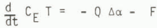
Q Δα denotes the effect of albedo changes on the net solar input, including variations of snow/ice cover or of cloud cover. The change of the infrared flux ΔF can be written as

following Reference WattsWatts (1980), Here, Y_j denotes all factors of influence except carbon dioxide, for instance surface temperature T, water vapour concentration or cloud cover, c is the CO₂ concentration, c₀ its preindustrial value. The last term takes into account the approximate variation of the infrared flux with the logarithm of the CO₂ concentration. Equation (2) can now be written as:

(3)

with the sensitivities

(4)

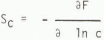
and

(5)

The numerical values for these sensitivities were taken from the radiative-convective model results of Reference Augustsson and RamanathanAugustsson and Ramanathan (1977) which include a positive water-vapour feedback process (constant relative humidity profile) and consider possible variations of cloud top altitude. They obtained, as extreme values for S_T, 2.24 W m⁻² K⁻¹ for constant cloud top altitude CTA and 1.38 W m⁻² K⁻¹ for constant cloud top temperature CTT. The CO₂ sensitivity of the flux appears to be relatively well established, and the value S_c = 6.4 W m⁻² is accepted here. Once radiative equilibrium has been reached, the heat storage term in Equation (3) vanishes and the new equilibrium temperature differs from the original temperature by:

(6)

For a CO₂ doubling, this yields, with the figures for S_c and S_T given above, a temperature increase of 1.98 and 3.21 K for constant CTA and constant CTT, respectively (Table I).

Table I Heat Flux Parameters and Equilibrium Temperature Changes for CO₂ Doubling for the Two Model Cases (CTA: cloud top altitude, CTT: cloud top temperature)

1.3 Heat storage and transport on Earth

The left-hand term of Equation (3), (d/dt) C_ET, denotes heat storage changes on Earth. It is easy to see that the main contributor to heat storage is the ocean. The atmospheric heat capacity per m² of Earth surface is 1 × 10⁷ J m⁻² K⁻¹, that of a 100 m thick layer of ocean water is 3.0 × 10⁸ J m⁻² K⁻¹, taking into account that the ocean covers the fraction f =0.71 of the Earth’s surface. For the continent, the penetration depth of the CO₂-induced warming is h_k = , where K_k is the diffusivity of heat and τ = 22.5 a is the e-folding time of the observed CO₂ increase. (As long as the relative CO₂ excess is smaller than about 20%, the temperature response to an exponential CO₂ incease is also approximately exponential, and the penetration depth is . This is found from Equation (3) when developing ln(c/c₀)). The effective heat capacity of the continent per m² of Earth surface, then, is h_k ρ C_k (1-f) = 1.2 × 10⁷ J m⁻² K⁻¹ (h_k = 19 m), using the values indicated by Reference Hoffert, Callegari and HsiehHoffert and others (1980), i.e. K_k = 16 m² a⁻¹, ρ=2 800 kg m⁻³ and C_k = 750 J kg⁻¹ K⁻¹ (specific heat). In other words, the heat capacities of the atmosphere and of the continents correspond to that of ocean layers of about 3 m and 4 m in depth, respectively, while the total penetration depth into a box-diffusive ocean with a mixed layer of 75 m and an eddy diffusivity of K = 4 005 m² a⁻¹ is of the order of 75 m + = 375 m. In the model simulation, therefore, only the oceanic heat capacity is considered.

In determining the mean global temperature change, different possibilities may be considered for taking into account the continental surface. First, we set the temperature change of the continents equal to that of the sea surface, which would correspond to a coupling coefficient υ = ∞ in Reference Cess and GoldenbergCess and Goldenberg’s (1981) terminology. This implies that the continental temperature change is driven fully by the temperature of the sea surface, or, in the one-dimensional boxdiffusion model, by that of the mixed layer. In this model, the heat balance (per m² of Earth surface) for the mixed layer reads, using Equation (3):

(7)

where T_s is the sea-surface temperature, f = 0.71 is the oceanic fraction of the Earth’s surface, h_m = 75 m the mixed layer depth, C_w the specific heat and ρ the density of sea-water, K. the eddy diffusion coefficient describing the vertical exchange rate in the deep sea (assumed to be the same for heat as for water or carbon) and

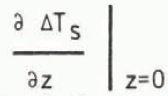
is the gradient of the temperature perturbation at the top of the deep-sea reservoir. The transport within the deep sea is governed by the same formulae as valid for CO₂, given by Reference Oeschger, Siegenthaler, Schotterer and GugelmannOeschger and others (1975). In contrast to the case of CO₂, there is no separate heat balance equation for the atmosphere, because its heat capacity is set to zero and the global surface temperature change is, in the model, equal to the change in the mixed layer.

2.1 Step increase of forcing

The transient heat storage of the model is well characterized by considering a step increase of an external forcing mechanism, e.g. a sudden increase of atmospheric CO₂.

In Figure 1 the result of the box-diffusion simulation for a stepwise CO₂ doubling is shown for constant CTT (cf. Table I). In the first 10 or 20 a, the temperature increases rapidly and reaches half the final value (1.6 K) after 27 a. After this initial period, however, it changes more and more sluggishly. After 100 a, the change is 69% of the equilibrium value of 3.21 K. The precise numbers depend on the values chosen for the model parameters and should not be considered as realistic. An important feature is, however, that equilibrium is not approached in an exponential way, as would be the case for a constant heat capacity. Rather the characteristic time scale, defined by ΔΤ_eq (d∆T/dt)⁻¹ increases with time, as does the effective heat capacity of the ocean. This reflects the characteristic behaviour of the box-diffusion model which for CO₂ was discussed by Reference Siegenthaler and OeschgerSiegenthaler and Oeschger (1978). The mixed layer and the upper deep-sea layers are rapidly warmed up, but it takes a very long time until the whole ocean has reached the new temperature. Until this is the case, however, heat is still transported downwards and the surface temperature is below its equilibrium value. In view of the very long time needed for reaching the equilibrium temperature, the effect of oceanic thermal inertia is not only a delay but actually also an attenuation of the temperature increase on the time scale of centuries.

Fig. 1 Transient response (solid line) of mean global surface temperature to a CO₂ doubling at time 0, using the box-diffusion model and assuming constant cloud top temperature (CTT). Dashed line: equilibrium response.

2.2 Temperature response due to fossil-energy induced CO₂ increase

Of interest is, of course, the predicted temperature rise due to the observed CO₂ increase. For this purpose, this increase was simulated by means of the box-diffusion model using the CO₂ production data of Reference RottyRotty (1983) as model input. Because here the effect of the actual CO₂ rise is of interest, the model was adapted so as to reproduce the observed CO₂ concentration (1 January 1959: 315.6 ppm, 1 January 1978: 333.8 ppm (Reference Bacastow, Keeling and BolinBacastow and Keeling 1981) by assuming a (small) additional CO₂ sink proportional to the fossil production rate. The pre-industrial level (constant until 1860) was assumed to be 296.9 ppm or about 297 ppm. The results for radiative equilibrium and for the transient system are represented in Figure 2 and for 1980 in Table II(a) both for constant CTA and constant CTT. If we consider these two cases as limits, then the temperature increase computed with oceanic heat capacity is between 0.20 and 0.26K in 1980 or roughly 50% of the equilibrium value. The corresponding time delay is between 16 and 24 a. The effect of the oceanic heat capacity (attenuation by about a factor of two) is relatively strong if compared to other estimates. This is related to the method of calibration of the ocean model using bomb-produce ¹⁴C, which yields a relatively large vertical diffusivity (7 685 m² a⁻¹) and is probably more applicable to the time scales considered here than a calibration using the natural ¹⁴C distribution.

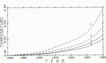
Fig. 2 Transient (solid lines) and equilibrium (dashed lines) temperature response to a CO₂ increase starting from 297 ppm in 1860, i.e. assuming fossil input only. Curves 1, 3: constant cloud top temperature (CTT), curves 2, 4: constant cloud top altitude (CTA).

Table II Equilibrium and Transient Temperature Increase for the Co₂ Increase Until 1980, and Delay of ΔT Compared to ΔT_eq (CTA: V constant cloud top altitude, CTT: V constant cloud top temperature)

a) Fossil input only (c₀ = 297 ppm)

2.3 Consequences of a low pre-industrial CO₂ concentration

Measurements on air bubbles occluded in old polar ice have yielded strong evidence that the pre-industrial CO₂ concentration was significantly lower than the value of 290 to 295 ppm previously assumed (Oeschger and others in preparationFootnote *). This implies that there must have been a large non-fossil input of CO₂ in the past, between about 50 and 150 a ago. Here we consider the consequences for the global temperature trend. For this purpose it was assumed that the concentration was 265 ppm until 1820; then it increased as a quadratic function of time to 273 ppm in I860, rose linearly to 313 ppm in 1955 and from then on followed the same curve as assumed in the last paragraph (fossil input only). The resulting transient temperature changes are presented in Figure 3 (upper two curves) for constant CTT and CTA, together with the corresponding curves for fossil input only (lower two curves); values for 1980 are given in Table II(b). Corresponding to the higher CO₂ increase until 1980 (27% of the preindustrial value instead of 13%), the computed temperature changes are roughly twice as large as in the 297 ppm (fossil-only) case. Again the attenuation due to the oceanic heat uptake is considerable, but it is not as strong as in the 297 ppm case because the CO₂ has increased more slowly in the 265 ppm case, according to our assumption, than in the first case, so that the ocean has had more time to warm up.

Fig. 3 Transient (solid lines) and equilibrium (dashed lines) temperature responses for CO₂ increase starting at 297 ppm (fossil input only, curves 3, 4) and at 265 ppm (early nonfossil input, curves 1, 2). Constant CTT is assumed.

Table II b) Lower pre-industrial value (c_o = 265 ppm)

2.4 Comparison with observed temperature trend

The observed hemi spheric or global trends of surface air temperature, as compiled by different authors, exhibit considerable short-time scatter, as well as long-term trends, for instance a cooling after 1940, which cannot be explained by CO₂ variations alone. This is not surprising and documents that other causes, such as volcanic dust or changing insolation, influence the air temperatures. Never-theless it is interesting to compare the observations with the computed trends due to CO₂. In Figure 4, anomalies of the mean surface temperature for the northern hemisphere since 1880, as calculated by Reference Jones, Wigley and KellyJones and others (1982), are shown, together with model-simulated curves for pre-industrial concentrations of 265 and 297 ppm (constant CTT, transient case). Since the observed data are not for the whole Earth but for the northern hemisphere only, the model curves shown were calculated for equal ocean and continent areas (f = 0.5), in contrast to those of Figures 1 to 3 that were obtained using f = 0.71. The model curves have been shifted so that their mean values for the period 1880–1980 are zero, as is the case for the observed anomalies. The comparison shows that the simulated curve for C₀ = 265 ppm can in principle explain an observed long-term warming of about 0.5 K between 1890 and 1980 (the decade between 1880 and 1890 seems to have been unusually cold and should therefore not be given much weight). The model curve for fossil input only (c₀ = 297 ppm) can explain less of the observed variations than the other model curve, in magnitude as well as in shape. In view of the large residual scatter it cannot easily be decided if this difference is significant. In order to determine whether the observed overall warming is due to CO₂ or not, it would be necessary to explain the residual variability. Attempts in this direction have been undertaken, invoking volcanic dust and solar variability (Reference HansenHansen and others 1981), but at present the experimental data are uncertain for volcanic forcing and only speculative for solar variability.

Fig. 4 Observed mean northern hemisphere temperature anomalies (Reference Jones, Wigley and KellyJones and others 1982). Dashed lines: transient mean global temperature changes simulated for pre-industrial values of 265 and 297 ppm. Constant CTT is assumed. All three curves have been shifted so as to have a mean value of zero in the period 1980 to 1980.

3.1 Heat exchange between ocean and continent

The transport of sensible and latent heat by the atmosphere provides for a quasi-continuous energy exchange process between continents arid ocean surface. In the following, we consider in a schematic way the case that this exchange flux is finite. We make the simple assumption that the exchange flux F_SC is proportional to the difference between the mean temperatures T_s and T_c of sea surface and continent:

(8)

where k_SC is a heat transfer coefficient (units: W m⁻² K⁻¹). It is assumed constant, which is an over-simplification since evaporation and hence latent heat transport strongly depend on temperature, but for a first sensitivity study it may be acceptable. We assume that ocean and continent cover the same area, which approximately holds for mid-latitudes in the northern hemisphere, so that the same transfer coefficient k_sc (per unit area) applies for the continent and for the sea.

The heat balance for the oceanic mixed layer now is given by

(9)

(cf. Equation (7)).

For the continent we have

(10)

Instead of the forcing by CO₂, any other external perturbation of the energy balance e.g. the seasonal variation of insolation can be inserted as the first term on the right-hand side of Equations (9) and (10). This provides a means to estimate the magnitude of the transfer coefficient k_sc. Using as a forcing term the expression S_T ΔΤ₀ sin ωt, with ω = 2∏ a⁻¹, yields expressions for the seasonal temperature variations; ΔΤ₀ would be the temperature amplitude in the absence of any internal heat fluxes. In midlatitudes of the northern hemisphere the ratio of the mean annual temperature amplitudes of continent and sea surface is 4 ± 1, as estimated from figure 7.20 of Reference Wallace and HobbsWallace and Hobbs (1977). For solving the equations equivalent to (9) and (10), we take into account only the mixed-layer heat capacity (h_m = 75 m), since the seasonal variations hardly penetrate into the thermocline. Formally, this is equivalent to setting K = 0 in Equation (9). With an average value of 1.7 W m⁻² K⁻¹ for S_T (the exact value of S_T is not essential) we obtain

for continent/ocean amplitude ratios of 3/4/5, respectively. For the numerical computation, the value 7.2 W m⁻² K⁻¹ has been used. An atmospheric thermal relaxation time can be calculated as C_a/k_sc, where C_a is an effective atmospheric heat capacity. Assuming that the layers below 500 mbar effectively contribute to the heat transport, C_a = 0.5 × 10⁷ W m⁻² K⁻¹•, and the relaxation time is eight days which appears a reasonable value.

3.2 Results

Transient temperature responses were computed for ocean and continent for the two CO₂ scenarios starting with 297 and 265 ppm, respectively. The results are plotted in Figure 5. The oceanic temperature change (solid line) is slightly smaller than the corresponding change on the continent (dashed line). The difference in 1980 is 10% for c₀ = 265 ppm and 151 for c₀ = 297 ppm; the relative differences would be slightly larger if constant CTA, instead of CTT had been assumed.

Fig. 5 Transient temperature changes calculated separately for continent (dashed) and ocean (solid curves), assuming a pre-industrial value of 265 ppm (curves 1, 2) or 297 ppm (curves 3, 4).

The simulated difference between ocean and continent is not large, but it is significant. In our model the ocean-continent heat coupling has been simulated 1n a very crude way, and the actual heat transfer flux may be different from the value determined here in an approximate way only (e.g. not con-sidering the influence of ocean circulation on seasonal sea-surface temperature variations).

Although the precise result for the temperature difference ocean-continent should not be given much weight; it is large enough to warrant further inspection. Reference Schneider and ThompsonSchneider and Thompson (1981) discussed the transient climatic response with respect to latitudinal differences. According to their model the approach towards equilibrium was significantly different in different regions, implying that the horizontal temperature gradient, and therefore the distribution of climatic change, might vary considerably from that determined, assuming equilibrium. (See also Reference Bryan, Komro, Manabe and SpelmanBryan and others 1982 and Reference Thompson and SchneiderThompson and Schneider 1982 for further discussions.) This argument also applies for the distinction ocean-continents. A continuing CO₂ growth, mainly if it. will be rapid, will imply ocean-continent differences, possibly leading to changes in atmospheric circulation.

All values (of Figure 5) are larger than those for the mean global temperature increase shown in Figure 3. The reason is that those curves were calculated with a value f = 0.71 for the oceanic fraction of the Earth’s surface area, while for Figure 5 (and Figure 4) equal oceanic and continental areas are assumed (f = 0.5). The results for the mean global temperature change with f = 0.5 (see Fig.4) are a few percent higher than those for the sea surface alone, as one would quantititively expect.