


Introduction
Temperature at the snow/soil interface strongly affects physical and biogeochemical processes that occur in snow-dominated environments. Cooling at the interface of shallow snowpacks allows freezing of the soil and retards infiltration at the beginning of snowmelt (Reference Dunne and BlackDunne and Black, 1971), and temperature influences carbon and nitrogen exchange (Reference Williams, Hood and CaineWilliams and others, 2001). The temperature at the interface can vary significantly spatially and temporally (Reference Hirota, Pomeroy, Granger and MauleHirota and others, 2002; Reference Cherkauer and LettenmaierCherkauer and Lettenmaier, 2003). Traditional measurements of snow and soil temperature profiles have often relied on vertically installed thermistors or thermocouples. While high temporal sampling can be achieved with such instruments, the spatial coverage is limited by logistical difficulties of wiring. Recent advantages in low-cost, self-organizing sensing platforms (Reference Akyildiz, Su, Sankarasubramaniam and CayirciAkyildiz and others, 2002) offer advances in the number of spatial measuring points; however, these continue to provide point measures of temperature rather than a comprehensive elucidation of the distribution of temperature.
Remote sensing of snow and land surface skin temperature offers fine spatial resolution across a snow or mixed snow/ soil surface. Forward-looking infrared imaging (FLIR) can provide meter-scale temperature resolution in fairly complex terrain (Reference Loheide and GorelickLoheide and Gorelick, 2006) but it cannot measure temperature beneath the snow surface. In snow-covered landscapes, FLIR also requires consideration of spatial, temporal and angular variability in emissivity not typically found in other environments (Reference Dozier and WarrenDozier and Warren, 1982).
Fortunately, new approaches in spatially distributed temperature sensing offer advantages. One such technique, Raman-spectra distributed temperature sensing (commonly referred to as ‘DTS’), developed in the 1980s (Reference Dakin, Pratt, Bibby and RossDakin and others, 1985; Reference Kurashima, Horiguchi and TatedaKurashima and others, 1990), has had wide application for sensing of temperature in harsh industrial environments including oil pipelines and boreholes, electric transmission cables and nuclear power plants (e.g. Reference FernandezFernandez and others, 2005). As the cost of the instruments has decreased and technology has improved, their application for environmental monitoring has blossomed (Reference SelkerSelker and others, 2006b; Reference WesthoffWesthoff and others, 2007), with preliminary foci on groundwater borehole logging and stream/groundwater interaction (Reference Selker, van de Giesen, Westhoff, Luxemburg and ParlangeSelker and others, 2006a). In these studies, the fine spatial (typically 1–2 m) and temporal (typically 10–60 s) resolutions have provided insights into local-scale processes that were impossible to resolve with traditional thermal monitoring instruments.
In this work, we expand the realm of DTS to the monitoring of snow basal temperatures in complex terrain. Our objective in the 2007 snow season was to test the suitability of the instrumentation and to examine fine-scale variability in the late snowmelt season. We begin with a brief overview of the Raman-spectra DTS theory and instrumentation, followed by a description of the study sites and an analysis of data recovered during spring melt. We conclude with recommendations for future installations and also suggestions for additional applications.
A Brief Overview of DTS Theory and Instrumentation
Detailed descriptions of DTS theory and sensors are available in the literature (Reference Dakin, Pratt, Bibby and RossDakin and others, 1985; Reference Kurashima, Horiguchi and TatedaKurashima and others, 1990), as are descriptions of hydrologic applications (Reference Selker, van de Giesen, Westhoff, Luxemburg and ParlangeSelker and others, 2006a, Reference Selkerb), but a brief overview is useful here. As coherent (laser) light is passed through an optical fiber, most of the energy is transmitted with no interactions with the quartz (SiO2) glass fiber or its impurities. However, a small fraction of the light is scattered by the fiber’s density variations, which are smaller than the wavelength of the incident light. Most of the backscattered energy is elastic, and hence returns at the incident wavelength (Rayleigh scattering). However, a small portion of the backscatter is inelastic, termed Raman and Brillouin scattering. Raman scattering generates light displaced both up and down in wavelength by the resonant frequency of the grid oscillations of the SiO2 bond structure. That energy scattered at shorter wavelength (termed anti-Stokes) strongly depends on the temperature of the SiO2 molecules of the fiber, while the energy scattered to the longer wavelength (Stokes frequency) is almost completely independent of the temperature. By comparing the ratio of anti-Stokes and Stokes intensities, the fiber-optic temperature can be calculated. The location along the cable of that temperature measurement is estimated by the time of flight of the incident light and scattered light. Figure 1b shows a typical Raman-scattered intensity from a fiber-optic cable at the snow/sediment interface, along with the resolved temperatures (Fig. 1a). Highly elevated temperatures occur where the fiber was exposed because the snowpack had already melted away. The general decline in signal intensity with fiber length is typical of energy dissipation in optical fibers, while the sharp declines in intensity seen at ∼50 and 60 m indicate anomalous light loss.
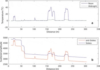
Fig. 1. Typical temperature (a) and Raman-scattering signals (b) from a fiber-optic cable during snowmelt. (a) demonstrates the ability of the system to detect large temperature changes over short distances; (b) shows the impact of temperature on the ratio of the Stokes and anti-Stokes scattered signal. The step changes in amplitude at 50 and 60 m in (b) represent attenuations caused by sharp bends or kinks in the cable.
Raman-scattering DTS uses the fiber-optic cable as a thermal sensor. No ‘sensors’ are added to the fiber, and inexpensive telecommunications multimode fiber can be used for many environmental applications. Typical commercial DTS instruments can resolve thermal variations of ±0.1°C, with some reports showing detection of 0.01°C changes at spatial scales of 1–2 m (Reference Selker, van de Giesen, Westhoff, Luxemburg and ParlangeSelker and others, 2006a). The total length of fiber to be interrogated can range from 100 m up to 30 km, with almost no limitation in the orientation of the fiber. While the environmental applications to date have used fiber lengths from 500 m to 2 km, it is probable that as the use of the DTS for environmental monitoring expands, much longer runs of fiber will be used to provide a dense grid network of temperature monitoring.
Study Sites and Instrumentation
Two study sites were chosen for the first applications of DTS technology to measure basal snow temperatures: the cooperative snow study site at Mammoth Mountain (37°37′ N, 119°02′ W; 2940 m a.s.l.) in the eastern Sierra Nevada, California, USA, and the Dry Creek Experimental Watershed (DCEW; 43°41′ N, 116°08′ W), Boise Mountains, Idaho, USA.
Mammoth Mountain
Measurements at the Mammoth Mountain site include incoming and outgoing solar and longwave radiation, air temperature, relative humidity, wind speed and direction, precipitation and snowfall, temperature at various depths in the soil and snowpack, and snowmelt runoff beneath the pack (http://neige.bren.ucsb.edu/mmsa/description.html).
In November 2006, before snowfall, a 300 m standard military telecommunications cable (Optical Cable Corp., 2-50/125 PE Jacketed Military Tactical B-Series Breakout cable) was deployed in a spiral pattern over a 0.25 ha (0.0025 km2) area surrounding the instrument shelter, passing over exposed bedrock and loosely anchored to shrubs and other obstructions. The fiber was protected from damage by a combination of Kevlar strength elements and polyurethane waterproofing elements. The 3 mm diameter of the fiber has very low thermal inertia and therefore responds quickly to temperature changes. Because the cable lacked crush-resistant elements (typically stainless steel), there were concerns over possible rodent damage in the field. However, the low cost of the cable (∼$1.70 m−1 including connectors) and the proof-of-concept objective of the experiment were primary factors in its choice. The two ends of the cable were terminated in the instrument shelter.
Within several days of deployment, a large windstorm with only minimal snowfall unfastened much of the cable and produced several intricate tangles and tight bends, which may have affected performance. The cable was redeployed and re-anchored and Figure 2a shows the final layout. All turns of the cable were staked such that the bend radius was greater than 30 cm to avoid signal loss. Shortly following the second deployment, snowfall buried the entire cable for the duration of the winter.
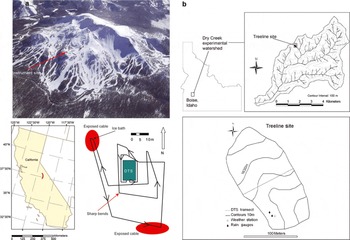
Fig. 2. Plan views of the two instrument sites, showing fiber deployment pattern. (a) Mammoth Mountain site, where the fiber is highlighted in red for those portions that traversed bare ground; and (b) DCEW.
In April 2007, a Sensornet Sentinel LR (Sensornet Ltd, London, UK) DTS unit, with a manufacturer’s stated resolution of ∼0.1°C at a range of 1000 m at a 10 s integration time, was set up in the instrument shelter and connected to the cable. The Sentinel LR is a stand-alone measurement, analysis and storage system, with a nominal power consumption of ∼105 W. Individual 10 s integrations are reported here. Resolution can be increased to better than 0.05°C by increasing integration times during measurement or during post-processing by averaging sequential measurements. During the period of measurement, most of the cable was buried by 1–2 m of snow, with four sections of cable (∼10–15 m, ∼100 m, ∼150–175 m and ∼220–240 m) traversing areas of bare dark volcanic rock or light-colored volcanic soil.
DTS surveys can be conducted in a variety of cable configurations, with significant implications regarding measurement noise and robustness. Though, in general, dual-ended measurements are preferred, we were only able to conduct single-ended measurements, because the particular DTS instrument used for this testing (Sentinel LR) was a single-channel instrument. As there were two fibers in the cable (and hence four ends), preliminary measurements were taken in both fibers and from both terminations to determine which of the four connectors had the lowest loss in light transmission. Light loss through cable connectors and junctions reduces the available returning Stokes and anti-Stokes signal and it is advisable in the field to use the best transmitting connectors. The connectors had not been kept well sealed over the winter period, and the connector with the least light loss was used for all of the data reported here.
Initial calibration of any DTS unit typically requires one or more sections of the fiber where the temperature is known. The calibration procedure consists of determining a temperature offset and a slope correction to account for differential losses of the Stokes and anti-Stokes signals in the fiber. For this work, a 0°C ice/slush bath was used for the temperature offset correction at the beginning of the experiment and as a check at the end of 24 hours of temperature logging on a section of fiber from 155 to 170 m. The slush bath was logged with a high-resolution (±0.001°C) digital thermometer (model No. 61220-601, VWR, Inc.) and remained at 0 ± 0.003°C during the calibration period. The Sentinel DTS can use on-board PT100 thermistors for reference, but also allows input of known temperature. The temperature-offset multiplier required to set the slush-bath temperature to 0°C was 0.9947, and the cable manufacturer’s differential loss coefficient was taken as 0.262 dB km−1. In single-end operation, it is advantageous to have at least two portions of the fiber at the same temperature to measure directly the differential loss coefficient, typically by looping the fiber back on itself to directly calculate the loss coefficient. Unfortunately, the crossover points on the cable were not precisely known (to accuracies less than 1 m) and the manufacturer’s loss coefficient was used instead.
Dry Creek Experimental Watershed
The study site is located in the 0.02 km2 Treeline site within the DCEW (Fig. 2b). The site has a mean elevation of 1620 m and local relief of 55 m (Reference McNamara, Chandler, Seyfried and AchetMcNamara and others, 2005). Both the northeast- and southwest-facing aspects of the study transect slope steeply at about 20°, with greater slopes toward the bottom, before converging in a narrow valley with essentially no riparian zone. In some years the Treeline site holds a persistent snowpack from around early November through March, while in warm years precipitation can fall mostly as rain. The stream draining the Treeline site is ephemeral and typically begins flowing soon after the onset of seasonal precipitation each year. Instrumentation at the Treeline site includes a weather station located on the northeast-facing slope recording incoming shortwave radiation, net longwave radiation, air temperature, relative humidity, wind speed and direction, precipitation using shielded and unshielded tipping-bucket gages, snow depth at one point, and soil temperature and soil moisture at depths ranging from 5 to 100 cm.
The Treeline site was free of snow in mid-February 2007 (Fig. 3). In late February, however, a winter storm system deposited approximately 50 cm of new snow at the site. During the initial stages of the storm, an 85 m section of a fiber-optic cable approximately 550 m long was deployed in a transect across the Treeline site (Fig. 2b). The transect was laid from the southwest to north ridges spanning 35 m of a northeast-facing slope and 50 m of a southwest-facing slope and was buried 1–2 cm below the ground surface.
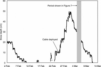
Fig. 3. Snow depth measured at one point on the northeast-facing slope of the Treeline site in the DCEW.
An Agilent N4386A DTS system collected single-ended measurements at 10 min intervals with a 30 s integration time at 1 m spatial resolution. The Agilent N4386A was connected to a laptop computer for data storage, and the DTS unit alone has a nominal power consumption of <20 W for operation from 0 to 20°C. Measurements began after the storm ceased. Due to the timing of the event, we were unable to calibrate the cable before deployment. Instead, we relied on a previously determined calibration, made with this Agilent instrument, of an identical cable. The fiber used was similar to that used at the Mammoth site, ∼3 mm 50/125 μm two-fiber cable fitted with E2000 connectors and angle polished cuts; however, the fiber was armored with Kevlar and stainless-steel strength elements and polyethylene waterproofing elements (Kaiphone Technology Co., Ltd, 50/125 PE Jacketed Armored Optical Fiber Cable).
Results
Mammoth Mountain
Figure 4 shows the temperature of fiber taken throughout the course of ∼24 hours at the Mammoth site. The calibration section of the fiber is clearly visible from ∼155 to 170 m of fiber as a step drop in temperature at ∼1100–1200 h on the first day and as a check on the second day of the experiment. The mean temperature over the entire calibration period, and averaged along the length of the calibrated fiber, is 0.04 ± 0.17°C. Alternatively, the temporal stability of the instrument can be estimated from the time average response of a point on the fiber in the bath (e.g. 165 m from 1100 to 1130 h), which shows a temperature of 0.07°C and a temporal standard deviation of ±0.14°C. The slightly higher standard deviation over distance is likely due to spatial averaging of the cable as it entered and exited the ice bath, since the entire 15 m section was used to calculate the standard deviation. The observed temperature resolution, as measured by all standard deviations, is about 1.5 times the stated resolution for the instrument. This may be due to the short section used for calibration. The manufacturer recommends a minimum 10 m calibration section, and we have found in subsequent work that at least 20–40 m of calibration section provides more stable calibration. Much higher temperature resolution than is reported here can be obtained for longer integration times and may be appropriate for snow installations where snow temperatures are changing rather slowly.
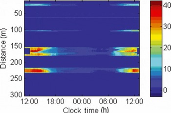
Fig. 4. Time-lapse image of the basal snow temperatures along the Mammoth cable. The two warmest sections are the areas where the fiber crossed bare ground. Short sections of the fiber were also exposed at ∼20 and ∼100 m and show as warm areas during midday. The circled portions of the graph indicate that portion of the fiber placed in the ice/slush bath for calibration.
Following calibration, measurements were taken for 10 s each 10 min for ∼24 hours, solar noon to solar noon. The four areas of cable exposure to sun are clearly visible, as are the calibration sections between 155 and 170 m. Air temperatures reached a maximum of 10.3°C, and portions of the exposed cable on bedrock reached over 40°C on the first day. During the second day of measurements, conditions were cooler (T max = 6.6°C) and much windier with intermittent clouds. As a result, the exposed bare ground and cable did not reach the maximum recorded the previous day. No independent measurements of the bare-ground/rock temperatures were made at MMSA, and it is probable that the dark color of the fiber resulted in slightly warmer temperatures in the fiber than the light-colored soils. However, qualitative measures, i.e. bare hands, of those areas where the fiber traversed dark volcanic rock did support the >40°C results.
Melting for the second day, as recorded by tipping-bucket lysimeters, continued and the rate of melting did not immediately respond to the decrease in temperature on the second day. However, melting did decrease by 80% on the day following the last DTS measurements, suggesting a significant lag in both melt response to temperature and travel times through the snowpack. Effects of shading on solar heating of bare ground can clearly be seen beginning at solar noon each day at a distance of ∼170 m down the cable.
Portions of the cable that remained buried by the snow stayed at 0°C during the entire experimental period, consistent with observations of melting snow and liquid-water content in the soil. Temperatures of the bare soil slowly cooled at night to 0°C and appear to have been held there by the surrounding snow and possible freezing of the soil. The minimum air temperature during the night was 2.6°C. Figure 5 shows temperature along bare ground (Fig. 5a) at 160 m and beneath snow (Fig. 5b) at 260 m as a function of time. The data clearly show the stability of the snow–soil temperatures and the highly varying bare-ground temperatures typically found in alpine and patchy snow-covered environments.
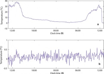
Fig. 5. Temporal changes in temperature at Mammoth Mountain: (a) cable located on bare ground; and (b) cable located at the snow/soil interface. Note the different temperature scales in the two graphs.
While the data appear consistent with isothermal conditions of the snowpack, closer inspection shows anomalous temperatures at the snow/soil interface for the first ∼60 m of cable. Figure 1a, showing temperature along the cable at 1622 h, displays three anomalous characteristics in the first 60 m. The measured snow–soil temperature averages −0.7°C for the first 60 m, excluding the recorded temperatures at ∼50 and 60 m. In a snow pit along the first 60 m, liquid water was present at the ground, and the interface temperatures were 0 ± 0.005°C. Moreover, two anomalous temperature spikes at 50 and 60 m were well below the snow surface and not subject to solar heating.
The anomalies can be explained by examining the raw amplitude data of the Stokes and anti-Stokes signals. Amplitude data (Fig. 1b) from the same period show two, step changes at 50 and 60 m. The temperature spikes at 50 and 60 m are likely the result of chromatic dispersion, in which the Stokes and anti-Stokes returns are improperly aligned in time, due to sharp changes in attenuation rate of the returning frequencies. As the temperature is calculated as the ratio of these amplitudes, any offset in time of their measurement can lead to an apparent temperature change. In a single-ended measurement design, as used at Mammoth Mountain, these localized losses lead to both an apparent temperature spike and, since the calibration bath was ‘downstream’ of the losses, an offset in the measured temperature. Field inspection after the snow had melted determined that the losses were most likely caused by sharp bends in the cable around small trees with bend radii of <5 cm. No losses were detected at the major turning points of the cable (Fig. 2a), as these bend radii were sufficiently large to avoid any light loss.
These types of losses along the fiber could have been corrected if the fiber had been interrogated in a double-ended manner. However, this was not possible with the instrument available in the field. Instead, for the Mammoth site, a simple constant offset can be applied to the data from 0 to 60 m to bring the average up to 0°C. In principle, since both Stokes and anti-Stokes data were retained, the chromatic dispersion could be corrected and the temperatures recalculated. It is highly advisable when conducting DTS studies to retain these data to assist in interpretation and to allow post-processing as needed.
Dry Creek Experimental Watershed
Temporal patterns of shallow soil temperature measured by the DTS were quite different on northeast- and southwest-facing slopes (Fig. 6). On the northeast-facing slope, soil temperatures remained relatively stable despite variable air temperatures (Fig. 7) through the 36 hour period owing to an insulating and melting snowpack. Snow depth decreased by approximately 10 cm (Fig. 3) but remained nearly contiguous through this period. Soil temperatures fluctuated between 1°C and 2°C, with the exception of the ridge top at approximately −28 m and at an anomaly at −24 m (discussed below). Soil temperature measured at the meteorological station on the northeast-facing slope also remained relatively stable, but near 0°C (Fig. 7). The apparent slight cooling of soil temperature that occurs when air temperature increases is not real, but is a function of solar radiation heating a reference thermistor used to calculate thermocouple temperatures. Because the soil temperature at 5 cm depth is near 0°C (Fig. 7) and the temperature at the snow/soil interface under a melting snowpack should be 0°C, we suggest that the temperature along the cable at 2 cm depth should also be 0°C. The difference is an offset that likely results from not calibrating the fiber optic but relying on previously determined calibrations of a similar cable.
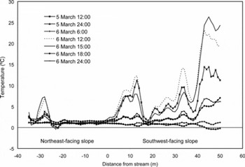
Fig. 6. Temperature distribution at the snow/soil interface across the Treeline site during a 36 hour period of active melting. The 0 m position is in the valley bottom stream. Negative numbers on the x axis advance up the north-facing slope, and positive numbers advance up the south-facing slope. Positions −30 m and +45 m are on relatively flat ridges.
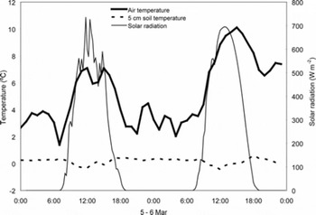
Fig. 7. Meteorological conditions on the northeast-facing slope of the Treeline site during the period shown in Figure 6. Soil temperature measurements were made with type T thermocouples referenced to a thermistor with an accuracy of 0.5°C.
The soil temperatures on the southwest-facing slope were much more responsive to air temperature than on the opposing slope (Fig. 6) owing to the thin, patchy snow cover. The amplitude of the response generally increases upslope, with occasional anomalies caused by local shading and the presence of a late-melting snowdrift at 17 m. The weaker response closer to the stream could be due to numerous factors including topographic shading from the northeast-facing slope, wetter soils near the stream, or steeper slopes near the stream. Note that the soil surface temperatures on the southwest-facing slope often exceeded air temperatures. For example, the ridge at the top of the southwest-facing slope (−48 m) reached 26°C on 6 March at 1500 h (Fig. 6), while the air temperature at the same time was only 10°C (Fig. 7). These warm temperatures are likely have a real component as the soil absorbs solar radiation, as well as an erroneous component caused by the black fiber-optic cable itself absorbing solar radiation.
At −24 m the cable shows an unusual and erroneous response; the lowest temperature occurs at 1200 h on 6 March, with warmer temperature during the subsequent night. This ‘overshoot/undershoot’ effect may be the result of sharp changes in real fiber temperature. Although the Stokes return is far less temperature-sensitive than the anti-Stokes, these changes result in small Stokes changes that were not sufficiently sampled in the early Agilent operating system. The Agilent DTS used a reduced bandwidth for the sensing of the Stokes signal in comparison to the bandwidth allocated for anti-Stokes sampling and it was not uncommon to see an ‘overshoot’ of the calculated temperature when the fiber underwent a step change in temperature, such as the fiber entering or leaving a constant-temperature bath. It is interesting, however, that the same problem does not occur on the southeast-facing slope at 17 m where the cable goes under a small snowdrift. Unlike the change at −24 m, the change in fiber temperature at 17 m was very localized beneath the snowdrift, and the spatial sampling of the DTS likely masked the overshoot/undershoot at this location. Current versions of Agilent DTS use a similar bandwidth for both Stokes and anti-Stokes, and such artifacts are no longer reported (personal communications from J. Dorighi and B. Nebendahl, 2007).
The different behavior of shallow soil temperature on the opposing slopes illustrates how point measurements in complex terrain can be highly affected by local environmental conditions. The DTS system can complement weather-station data and provide a mechanism to distribute point measurements of soil temperature for improved catchment-scale energy-balance studies.
Conclusions
The data collected over a couple of days in the spring 2007 snowmelt season show that Raman-spectra distributed temperature sensing is suitable for investigations of snow thermal processes. Long cable lengths can be laid out for either transects or x-y locations in complex terrain. The robust fibers survived the winter unbroken and undamaged by animals.
The two examples shown in this work demonstrate only part of the range of possible applications of DTS to snow. At the Mammoth site, melting conditions and the presence of bare ground during snowmelting were clearly seen. A uniform 0°C snow basal temperature was observed, consistent with the melting conditions and the appearance of liquid water at the base of the snowpack. The inexpensive fiber-optic cable proved to be resistant to failure over an entire winter season, and, where defects in the cable were observed (remotely), these could easily be corrected for in the data processing. The Dry Creek site showed the benefits of the high spatial resolution that DTS can provide. During snowmelt there, strong gradients in shallow soil temperature were observed that agreed well with catchment aspect and slope. The impact of patchy snow cover was easily seen in the temporal variation of the DTS temperatures along the southwest-facing slope of the catchment. Such local-scale variations in temperature could not be resolved from traditional measurements (soil thermocouples, weather stations, etc.) at the spatial resolution afforded by the DTS system.
In both examples, data collected in this study demonstrate the ‘worst case’ resolution of typical DTS instruments. Significant improvements in this resolution (down to ±0.05°C) can easily be obtained using integration times of 1–10 min and by making double-end measurements wherever possible. Fiber connectors were shown to be another ‘weak point’ of installations, and care must be given to keeping fiber ends clean and dry during experiments. The studies demonstrated the need to carefully install cable such that sharp bends are avoided and to insure that excessive loadings are avoided. Where cables are exposed to direct sunlight, care must be used in interpreting the reported temperatures, as differences in albedo between the cable and bare ground may result in anomalous heating or cooling of the cable. Calibration baths were also shown to be an essential part of any DTS installation, as the results from Dry Creek showed a 1°C offset in basal temperatures. The study suggests that >20 m lengths of fiber should be used for calibration baths, and that the design of calibration baths should be considered before installing cable. At the MMSA site, we were fortunate that the snowpack had melted in places to expose cable to be used in calibration.
Based upon the lessons learned from these two proof-ofconcept trials, resolution of snowpack temperatures can easily be improved to match those reported in other environmental applications of DTS systems. Future DTS installations are unlikely to be limited to basal temperature measurement. The development of vertical profile sensors (Reference Selker, van de Giesen, Westhoff, Luxemburg and ParlangeSelker and others, 2006a) and the potential to install small-diameter fiber within the snowpack either before or immediately after snowfall suggests that DTS can provide very high vertical and horizontal spatial resolution of snowpack temperatures to better understand snow thermal dynamics and snow evolution.
Acknowledgements
The authors greatly appreciate the valuable comments and suggestions from the two anonymous reviewers. Partial support for the research was provided by the US Bureau of Reclamation Agreement No. 06FC204044. The instrument station and snow property research on Mammoth Mountain is supported by US National Science Foundation grant EAR-0537327, the US Army Cold Regions Research and Engineering Laboratory, and the Mammoth Mountain Ski Area. The DCEW is jointly operated by Boise State University and the US Department of Agriculture Northwest Watershed Research Center. Research at the DCEW was supported by US National Science Foundation grant EPS-0447689.


