


1. Introduction
Vortices are key dynamical features of the atmosphere and the oceans. Collectively, they contribute to a significant part of the mass transport in the oceans (Zhang, Wang & Qiu Reference Zhang, Wang and Qiu2014). When two opposite-signed vortices are close together, they interact strongly and form a pair that self-propagates in the flow (de Ruijter et al. Reference de Ruijter, van Aken, Beier, Lutjeharms, Matano and Schouten2004; L'Hegaret et al. Reference L'Hegaret, Carton, Ambar, Menesguen, Hua, Chérubin, Aguiar, Le Cann, Daniault and Serra2014). Typically, the distance separating the vortices remains nearly constant in time, at least until the pair interacts strongly with another feature. Such pairs of vortices are sometimes referred to as dipoles, and they can transport momentum, mass and tracers efficiently over long distances in the fluid. Recent analyses of altimetry data have shown that dipoles are widespread in the global ocean (Ni et al. Reference Ni, Zhai, Wang and Hughes2020).
Dipoles also include mushroom-like currents that abound in the oceans (Fedorov & Ginsburg Reference Fedorov and Ginsburg1989). Other families of dipoles include modons on the  $\beta$-plane (Stern Reference Stern1975; Larichev & Reznik Reference Larichev and Reznik1976) and on the $f$-plane (Kizner et al. Reference Kizner, Reznik, Fridman, Khvoles and McWilliams2008), to name but a few examples. Other examples are the hetons introduced by Hogg & Stommel (Reference Hogg and Stommel1985) where the two opposite-signed vortices occupy distinct depths. These vortices will not be considered in the present paper.
Pallàs-Sanz & Viúdez (Reference Pallàs-Sanz and Viúdez2007) investigated numerically the ageostrophic motion of a specific family of pairs of opposite-signed vortices where the two vortices are ellipsoids of uniform potential vorticity. The authors showed that ageostrophic effects affect the trajectory of the dipole as the anticyclonic vortex tends to be larger and more intense. In their study, the vortices in the dipole remained well-separated and the vortices retained their volume.
In the present work, we determine numerically pairs of opposite-signed, uniform potential vorticity (PV) vortices in mutual equilibrium under the quasi-geostrophic (QG) approximation, for vanishing Rossby ( ${\textit {Ro}}$) and Froude ( ${\textit {Fr}}$) numbers, on the $f$-plane. These equilibria are then used to initialise numerical simulations at finite ${\textit {Ro}}$ and ${\textit {Fr}}$. This choice helps the vortices to remain close to an equilibrium for small ${\textit {Ro}}$, and therefore limits vortex deformations otherwise associated with another arbitrary choice of initial conditions. It also limits the spontaneous generation of inertia-gravity waves and allows the flow to remain close to a balanced state. We show that both under the QG approximation and at finite ${\textit {Ro}}$ and ${\textit {Fr}}$ numbers, the pair of vortices undergoes a destructive interaction when the distance separating them is less than a threshold that we determine. For non-destructive interactions, where the vortices retain their material, we quantify the dynamical asymmetry between the cyclonic and the anticyclonic vortices by measuring a QG-equivalent PV ratio. This is the PV ratio of a pair of QG vortices having the same trajectory.
The paper is organised as follows. Pairs of counter-rotating vortices in mutual equilibria under the QG approximation are presented in § 2. Section 3 is devoted to the nonlinear evolution of the vortex pairs at finite  ${\textit {Ro}}$ and ${\textit {Fr}}$ numbers. Conclusions are given in § 4.
2. Quasi-geostrophic equilibria
We first consider pairs of counter-rotating vortices under the QG approximation. Under this approximation, the full flow fields can be recovered from a single scalar field  $q$, the QG PV anomaly, hereinafter referred to as PV for simplicity. In the form used in this study, the QG equations are obtained by a Rossby number expansion of Euler's equations for a rotating fluid under the Boussinesq approximation with ${\textit {Fr}}^2 \ll {\textit {Ro}} \ll 1$. Here, ${\textit {Ro}}=U/(fL)$ is the Rossby number, while ${\textit {Fr}}=U/(NH)$ is the Froude number; $U$ is a characteristic scale of horizontal velocity, $f$ is the Coriolis frequency, $N$ is the buoyancy (or Brunt–Väisälä) frequency, and $L$ and $H$ are horizontal and vertical length scales, respectively. A complete derivation may be found in Vallis (Reference Vallis2006). For simplicity, we assume that both $f$ and $N$ are constant. The PV $q$ may be defined as the modified three-dimensional Laplacian of a streamfunction $\varphi$:
 \begin{equation} q = \frac{\partial^2 \varphi}{\partial x^2} + \frac{\partial^2 \varphi}{\partial y^2} + \dfrac{f^2}{N^2}\,\frac{\partial^2 \varphi}{\partial z^2} = {\mathcal{L}}_{QG}(\varphi). \end{equation}
 The PV  $q$ is conserved materially in the absence of diabatic or dissipative effects:
 \begin{equation} \frac{\partial q}{\partial t} + u\,\dfrac{\partial q}{\partial x} + v\,\frac{\partial q}{\partial y}= 0, \end{equation}
where the advecting velocity field  $\boldsymbol {u}=(u,v,0)$ is the non-divergent geostrophic velocity deriving from the streamfunction $\varphi$ as
 \begin{equation} u ={-}\frac{\partial \varphi}{\partial y}, \quad v = \frac{\partial \varphi}{\partial x}. \end{equation}
Finally the buoyancy anomaly is recovered from  $\varphi$ via
 \begin{equation} b=f\,\frac{\partial \varphi}{\partial z}. \end{equation}
It is important to notice that there is no dynamical asymmetry between a cyclonic vortex ( $q>0$) and an anticyclonic vortex ( $q<0$) in QG.
We consider two vortices of uniform PV  $\pm q_r$, with $q_r>0$ without loss of generality. We denote as vortex $1$ the vortex with PV $q_1= -q_r$, and as vortex 2 the vortex with $q_2=q_r$. The vortices have the same volume ${\mathcal {V}}_1={\mathcal {V}}_2={\mathcal {V}}$, hence the same strength in absolute value $|\kappa _1|=|\kappa _2|$, where $\kappa _i\equiv (4{\rm \pi} )^{-1} q_i{\mathcal {V}}_i$. We set $q_r=2{\rm \pi}$, implicitly defining a time scale for the problem. For example, the rotation period of a single sphere, in the $(x,y,zN/f)$ coordinate system, of uniform PV $q_r$ is $T=6{\rm \pi} /q_r=3$ here. Each vortex is centred at $\boldsymbol {x}_i$. We denote the vertical offset between the vortices as $\Delta z = z_2-z_1 \geq 0$ without loss of generality. Recall that the absence of vertical advection under the QG approximation implies that $z_i = {\rm const}$. The fluid domain is unbounded in all three directions of space.
We determine numerically the shape of the vortices in mutual equilibrium, translating steadily at a constant velocity  $V$ in the unbounded fluid domain. It should be noted that Reinaud & Dritschel (Reference Reinaud and Dritschel2009) have already determined equilibria for pairs of unequal-sized counter-rotating vortices, albeit at lower resolution. In this case, the pairs rotate rather than translate. The present choice of translating vortices is to emphasise the dynamical asymmetry due to ageostrophic effects discussed in § 3. In this present study and without loss of generality, the vortex centres are horizontally aligned along the $y$-direction and separated in the $x$-direction. Thus the vortices translate in the $y$-direction. The boundary of each vortex is discretised in the vertical direction by $n_c$ horizontal layers. In each layer, the vortex boundary is defined by a contour. For the pair of vortices, there are $2 n_c$ contours, denoted ${\mathcal {C}}_k, \,1\leq k\leq 2 n_c$. We use an iterative procedure that makes the contours ${\mathcal {C}}_k$ converge to streamlines in the reference frame translating with the vortices:
 \begin{equation} \tilde{\varphi}(\boldsymbol{x}) = \varphi(\boldsymbol{x}) - V x = C_k,\quad \forall \boldsymbol{x}=(x,y,z) \in {\mathcal{C}}_k, \end{equation}
where  $C_k$ is a constant depending on the contour ${\mathcal {C}}_k$, and $\tilde {\varphi }$ is the streamfunction expressed in the reference frame translating at velocity $V$. Details of the method may be found in previous works, e.g. Reinaud & Dritschel (Reference Reinaud and Dritschel2002) and Reinaud (Reference Reinaud2019). For a given vertical offset $\Delta z$, we start with vortices that are well separated in the horizontal direction by a distance $\Delta x_{init}$. The initial guess for the vortex shape is a sphere in the $(x,y,zN/f)$ coordinate system. This is motivated by the fact that a pair of spherical vortices infinitely separated in the horizontal direction would indeed be in equilibrium. Indeed, any axisymmetric vortex standing alone is a steady state. We can also note that all vortices in this study have a mean unit height-to-width aspect ratio in the $(x,y,zN/f)$ coordinate system.
We take  $x_1>0$ for the first equilibrium. When the equilibrium is reached, the vortices are pushed slightly together by a small distance $\delta '$, and the numerical procedure is resumed for the new horizontal separation. The procedure is repeated until the method fails to converge, corresponding to the end of the numerical branch of solutions. Hence, for a given $\Delta z$, we determine a family of equilibria spanned by the horizontal distance between the vortices. For this horizontal distance, it is convenient to use the innermost gap $\delta =x^m_1-x^m_2$, the distance between the two innermost edges $x^m_i$ of the vortices as shown in figure 1. Note that $\delta$ can reach negative values when the vortices are vertically offset.

Figure 1. Definition of the innermost gap  $\delta = x^m_1-x^m_2$, the signed distance between the innermost edges of vortex 1 and vortex 2. The cyclonic vortex ( $q>0$) is henceforth shown in red, while the anticyclonic vortex ( $q<0$) is shown in blue.
We also address the linear stability of the equilibria. Details of the method may also be found in previous works, e.g. Reinaud & Dritschel (Reference Reinaud and Dritschel2002) and Reinaud (Reference Reinaud2019). The method analyses the deformation modes of the vortex bounding contours by considering infinitesimal disturbances on the horizontal position vector  $\boldsymbol {\rho }_k(\tilde {\theta },t)$ of the nodes along the contour ${\mathcal {C}}_k$:
 \begin{equation} \boldsymbol{\rho}_k(\tilde{\theta},t) = \boldsymbol{\rho}_{e,k}(\tilde{\theta}) + \gamma_k(\tilde{\theta},t)\,\frac{(-\mathrm{d} y_{e,k}/\mathrm{d} \tilde{\theta}, \mathrm{d} x_{e,k}/\mathrm{d} \tilde{\theta})}{(\mathrm{d} x_{e,k}/\mathrm{d}\tilde{\theta})^2 + (\mathrm{d} y_{e,k}/\mathrm{d}\tilde{\theta})^2}, \end{equation}
where  $\boldsymbol {\rho }_{e,k}=(x_{e,k},y_{e,k})$ is the position vector at equilibrium, and $\tilde {\theta }$ is the ‘travel-time coordinate’, an angle proportional to the time taken by a fluid particle to travel along the contour ${\mathcal {C}}_k$. The disturbance $\gamma _k$ is taken in the form
 \begin{equation} \gamma_k(\tilde{\theta},t) = \mathrm{e}^{\sigma t} \sum_{m=1}^M \hat{\gamma}_{m,k} \, \mathrm{e}^{\mathrm{i} m \tilde{\theta}}, \end{equation}
where  $m$ is the mode's azimuthal wavenumber, and $M$ is the maximum wavenumber considered in the study. The evolution equation for $\gamma _k$ is given by
 \begin{equation} \dfrac{\partial\gamma_k}{\partial t} + \omega_k\,\dfrac{\partial \gamma_k}{\partial \tilde{\theta}} ={-} \sum_{l=1}^{2n_c} \Delta q_l\,\dfrac{\partial}{\partial \tilde{\theta}} \oint_{{\mathcal{C}}_l} \gamma_l \, G_{k,l}\left( \left| \boldsymbol{\rho}_{e,k}(\tilde{\theta})-\boldsymbol{\rho}_{e,l}(\tilde{\theta}') \right| \right) \mathrm{d} \tilde{\theta}', \end{equation}
where  $\omega _k$ is the constant rotation rate of a fluid particle along the contour ${\mathcal {C}}_k$, $\Delta q_l = \pm q_r$ is the PV jump across the contour ${\mathcal {C}}_l$, and $G_{k,l}$ is the Green's function giving the velocity induced in the layer containing the contour ${\mathcal {C}}_k$ in the layer containing the contour ${\mathcal {C}}_l$ in the unbounded fluid domain.
In this study, we set  $M=10$, which is enough to capture the onset of instability from previous experience (Reinaud & Dritschel Reference Reinaud and Dritschel2009). Substituting (2.7) into (2.8) results in a $4\times n_c\times M$ real eigenvalue problem where $\sigma =\sigma _r + \mathrm {i} \sigma _i$ is a complex eigenvalue. The real part $\sigma _r$ of $\sigma$ is the mode's growth rate, and the imaginary part $\sigma _i$ of $\sigma$ is its frequency.
In this study, we set  $n_c=83$ for a fine vertical discretisation of the vortices. Symmetry with respect to the plane $y=0$ is imposed. Half of each contour ${\mathcal {C}}_k$ is discretised using $n_p=330$ nodes to ensure high accuracy. The total volume of PV, in the $(x,y,zN/f)$ coordinate system, is set to $4{\rm \pi} /3$. The mean radius of each vortex in this coordinate system is therefore $r_v=(1/2)^{1/3}$. We denote $H=2r_v=2^{2/3}$ as the total height of each vortex. The vertical offset $\Delta z$ between the vortices is taken, for convenience, as a fraction, in number of layers, of the total height $H$. In this study, we consider $\Delta z /H=0, 21/83, 41/83, 62/83$, so offsets of $0$,
$0$,  ${\sim }25\,\%$, ${\sim }50\,\%$ and ${\sim }75\,\%$ of the vortex height. For each value of $\Delta z$, we start the calculation with $\Delta x_{init}=3$, and we used $\delta '=0.01$ between equilibria.
Figure 2(a) shows the translation velocity  $V$ of the vortex pair at equilibrium as a function of the innermost gap $\delta$. For $\Delta z=0$, the velocity increases monotonically as the gap $\delta$ decreases and the vortices interact more strongly. For $\Delta z \neq 0$, the velocity is no longer a monotonic function for the gap for $\delta < 0$. This can be explained easily by the fact that for a pair of opposite-signed QG point vortices, the translation velocity is $\propto \delta x/(\delta x^2+\delta z^2)^{3/2}$ – where $\delta x$ and $\delta z$ are the horizontal and vertical separations between the point vortices, respectively – and has an extremum for $\delta x = \delta z/\sqrt {2}$. In figure 2(a), $V$ is also affected by the shape of the finite-core vortices in equilibrium and the vertical overlap of the vortices for $\delta <0$. The translation velocity $V$ also decreases with the vertical offset $\Delta z$ as the vortices are further apart, weakening their interaction. Figure 2(b) shows the maximum growth rate $\sigma ^m_r$ versus the gap $\delta$. For all $\Delta z$, the pair of vortices is in a neutrally stable equilibrium with $\sigma ^m_r\simeq 0$ for large $\delta$. The residual non-zero values for large $\delta$ are due to the finite numerical accuracy of both the numerical determination of the equilibria and the linear stability analysis itself. As $\delta$ is further decreased, a first mode of instability, corresponding to $\sigma ^m_r>0$, appears at a critical value of the gap $\delta _c$ that depends on the vertical offset $\Delta z$. The values of $\delta _c$ are reported in table 1. As $\Delta z$ increases, the interaction between the vortices weakens for a given $\delta$, and $\delta _c$ decreases. It is, however, interesting to notice that the distance $d_{3D}$ between the two vortex centroids at the margin of stability, also given in table 1, increases with $\Delta z$. This shows that vortices are particularly sensitive to vertical shear, which is enhanced by increasing moderately the vertical offset $\Delta z$. A similar trend is observed at the margin of stability of pairs of co-rotating QG vortices (Reinaud & Dritschel Reference Reinaud and Dritschel2002, Reference Reinaud and Dritschel2005) and the importance of vertical shear is also shown in QG turbulence (Reinaud, Dritschel & Koudella Reference Reinaud, Dritschel and Koudella2003). Since the vortices exert on each other both horizontal and vertical shear, the instabilities have both barotropic and baroclinic components. We conjecture that for $\Delta z$ small, the instability is dominated by barotropic effects, while baroclinic effects increase continuously as $\Delta z$ is increased. For $\Delta z/H>1$ (not considered in the present paper), the pair of opposite-signed vortices is referred to as a heton, and the instability is mostly baroclinic in nature.

Figure 2. (a) Translation velocity  $V$ of the equilibria, and (b) maximum growth rate $\sigma ^m_r$, both scaled by the reference PV $q_r$, versus the innermost gap $\delta$ for the relative vertical offset $\Delta z=0$ (black lines) and $\Delta z/H= 21/83$ (red lines), $41/83$ (blue lines), $62/83$ (green lines).
Table 1. Critical gap  $\delta _c$ for the four values of relative vertical offset $\Delta z/H$ considered, and corresponding vortex centroid separation $d_{3D}$.
Figure 3 shows the shape of the vortices at equilibrium for the first unstable state, i.e. for  $\delta = \delta _c^-$, within the accuracy of $\delta '$, the gap increment between consecutive equilibria. Except for the case $\Delta z=0$, the vortices tilt with respect to the vertical direction. The vortices flatten in the $x$-direction, the direction along the axis joining the vortex centres, and elongate in the $y$-direction as the gap is decreased. Recall that the vortices have circular horizontal cross-sections as $\delta \to \infty$. Figure 4 shows the last equilibria found numerically for each $\Delta z$. We denote by $\delta ^*$ the corresponding value of the gap $\delta$. These states are strongly unstable.

Figure 3. Vortex bounding contours for the relative equilibria at the margin of stability, for (a)  $\Delta z/H=0$, (b) $\Delta z/H=21/83$, (c) $\Delta z/H=41/83$, and (d) $\Delta z/H=62/83$. The vortices are viewed orthographically at angle $60^\circ$ from the vertical direction, in the $(x,y,zN/f)$ coordinate system.

Figure 4. Vortex bounding contours for the last relative equilibria along the branch for  $\delta = \delta ^*$, for (a) $\Delta z/H=0$, (b) $\Delta z/H=21/83$, (c) $\Delta z/H=41/83$, and (d) $\Delta z/H=62/83$. The vortices are viewed orthographically at angle $60^\circ$ from the vertical direction, in the $(x,y,zN/f)$ coordinate system.
We next investigate the nonlinear evolution of the unstable equilibria. We use contour surgery with the standard set-up of the method (Dritschel Reference Dritschel1988; Dritschel & Saravanan Reference Dritschel and Saravanan1994). The method is purely Lagrangian and the fluid domain is explicitly unbounded, consistent with the equilibria. We start with the equilibria shown in figure 3 for  $\delta = \delta _c^-$. The contours bounding the vortices in mutual equilibrium are re-discretised using fewer nodes to reduce the computational cost of the contour surgery simulations while maintaining high accuracy. This re-discretisation introduces a small disturbance on the equilibria, enough to trigger the instability. The simulations are run until $t=100$. We determine diagnostically the locations of the vortex centres
 \begin{equation} \boldsymbol{x}_i = \dfrac{1}{{\mathcal{V}}_i} \iiint_{{\mathcal{V}}_i} \boldsymbol{x} \, \mathrm{d}^3\boldsymbol{x}, \end{equation}
and the semi-axis lengths,  $a\leq b\leq c$, of the best-fitted ellipsoids as functions of time. The best-fitted ellipsoid to a vortex is the ellipsoid having the same centre and the same second-order geometric moments as the vortex,
 \begin{equation} I_{mn} = \iiint_{{\mathcal{V}}_i} (x^m-x_i^m)(x^n-x_i^n) \,\mathrm{d}^3 \boldsymbol{x}, \end{equation}
where we denote  $(x,y,z)=(x^1,x^2,x^3)$ to simplify notations. Results are presented in figure 5. The values of the translation velocity $V/q_r$ of these specific equilibria are recalled in table 2. In all cases, the dipole starts by translating at a constant velocity $V>0$, and the vortices deform little: the semi-axis lengths $a,c,b$ remain constant initially. As the disturbances grow on the unstable equilibria, the vortices deform slightly as seen from the small variations of the semi-axis lengths in figures 5(b,d,f,h). This in turn affects their trajectories as seen in figures 5(a,c,e). For $\Delta z/H=62/83$, vortex deformation occurs mostly in the limited region where the vortices occupy the same horizontal layers, and the weak deformation has a limited effect on the vortex centre trajectories. For $\Delta z/H=21/83$, results are shown for $t \leq 85$ until a small debris detaches from vortex 2. The volume of the debris is only $1.6\times 10^{-6}{\mathcal {V}}_2$. In all the other cases, the interaction is non-destructive. The vortices deform but retain their material, at least until the end of the simulation $t=100$. It should also be noted that by $t=100$, the dipoles have nearly travelled the distance $L=V t$ that the undisturbed equilibria would have; see figures 5(a,c,e,g) and table 2. The instability hardly affects the dipoles overall, which is expected so close to the margin of stability.

Figure 5. Vortex centre trajectories (a) and best-fitted ellipsoid semi-axes lengths (b) for the unstable QG equilibria for  $\delta =\delta _c^-$ shown in figure 3(a) for $\Delta z=0$. Similarly, (c,d) for $\Delta z/H=21/83$, (e,f) for $\Delta z/H=41/83$, and (g,h) for $\Delta z/H=62/83$.
Table 2. Translation velocity  $V/q_r$ for the QG equilibria for $\delta =\delta _c^-$ shown in figure 3 and the distance $L = V t$ that the undisturbed equilibria would travel until $t=100$. $^{a}$At $t=85$.
We next turn our attention to the nonlinear evolution of the strongly unstable equilibria shown in figure 4, corresponding to  $\delta =\delta ^*$. In these cases, simulations are run until $t=50$. A snapshot on the vortices at
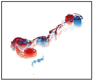
  $t=50$ is shown in figure 6. In all four cases, the interaction results in the destruction of the two vortices as they break into several secondary vortices and a plethora of PV debris and filaments. For small vertical offsets, the interaction forms a mushroom-like structure, e.g. $\Delta z/H=0$, $21/83$. For large vertical offsets, $\Delta z/H=41/83$, $62/83$, part of the secondary vortices resemble hetons, or baroclinic dipoles. It should be noted that there is no dynamical asymmetry between cyclones $q>0$ and anticyclones $q<0$ within the QG model. In the cases considered here, the two vortices are initially symmetric. Contour surgery does not, however, enforce symmetry. While the numerical noise does not disturb the vortices symmetrically, some degree of symmetry remains in the evolution of the vortices. The dynamical symmetry of the QG model breaks when adding the ageostrophic effects associated with a finite ${\textit {Ro}}$. This is the focus of § 3.

Figure 6. Vortex bounding contours for the nonlinear simulation of the unstable QG equilibria shown in figure 4 for  $\delta =\delta ^*$, for (a) $\Delta z/H=0$, (b) $\Delta z/H=21/83$, (c) $\Delta z/H=41/83$, and (d) $\Delta z/H=62/83$ at $t=50$. The vortices are viewed orthographically at angle $60^\circ$ from the vertical direction in the $(x,y,zN/f)$ coordinate system. The colour gradient indicates depth.
3. Finite  ${\textit {Fr}}$ and ${\textit {Ro}}$ vortices


We next consider the evolution of the pairs of vortices at finite  ${\textit {Fr}}$ and ${\textit {Ro}}$. Following Dritschel & Viúdez (Reference Dritschel and Viúdez2003), the prognostic equations are written in terms of Ertel's PV anomaly rescaled by $N^2$, $q$, which is conserved materially, and the horizontal part $\boldsymbol {A}_h$ of the vector quantity
 \begin{equation} \boldsymbol{A} \equiv \frac{\boldsymbol{\omega}}{f} + \frac{\boldsymbol{\nabla} b}{f^2}, \end{equation}
where  $\boldsymbol {\omega } = \boldsymbol {\nabla } \times \boldsymbol {u}$ is the vorticity, $b$ is the buoyancy anomaly, and $\boldsymbol {u}=(u,v,w)$ is the velocity.
The evolution equations for the variables  $q$ and $\boldsymbol {A}_h$ are
 \begin{gather} \frac{\mathrm{D} q}{\mathrm{D} t} =0, \end{gather}
 \begin{gather}\frac{\mathrm{D} \boldsymbol{A}_h}{\mathrm{D} t} + f \boldsymbol{k} \times \boldsymbol{A}_h = \frac{1}{f}\,(\boldsymbol{\omega} \boldsymbol{\cdot} \boldsymbol{\nabla}) \boldsymbol{u}_h + \left( 1 - \frac{N^2}{f^2}\right) \boldsymbol{\nabla}_h w - \frac{1}{f^2}\,\boldsymbol{\nabla}_h \boldsymbol{u} \boldsymbol{\cdot} \boldsymbol{\nabla} b, \end{gather}
where  $\mathrm {D}/\mathrm {D} t \equiv \partial /\partial t + \boldsymbol {u} \boldsymbol {\cdot } \boldsymbol {\nabla }$ is the material derivative, $\boldsymbol {k}$ is the vertical unit vector, and the subscript $h$ denotes the horizontal part of a vector quantity. We next define a vector potential $\boldsymbol {\varphi } = (\varphi, \psi, \phi )$ associated with the vector $\boldsymbol {A} \equiv \Delta \boldsymbol {\varphi }$. Then we have readily
 \begin{gather} \boldsymbol{u} ={-} f\,\boldsymbol{\nabla} \times \boldsymbol{\varphi}, \end{gather}
 \begin{gather}b = f^2\,\boldsymbol{\nabla} \boldsymbol{\cdot} \boldsymbol{\varphi}. \end{gather}
The inversion relations to obtain  $\boldsymbol {\varphi }$ are
 \begin{gather} \Delta\boldsymbol{\varphi}_h=\boldsymbol{A}_h, \end{gather}
 \begin{gather}{\mathcal{L}}_{QG}(\phi) - \left(1-\frac{f^2}{N^2}\right)\boldsymbol{\nabla}\boldsymbol{\cdot}\frac{\partial \boldsymbol{\varphi}_h}{\partial z} + \frac{f^2}{N^2}\,\boldsymbol{\nabla}(\boldsymbol{\nabla}\boldsymbol{\cdot}\boldsymbol{\varphi})\boldsymbol{\cdot} \left( \boldsymbol{\nabla}^2\boldsymbol{\varphi} - \boldsymbol{\nabla}(\boldsymbol{\nabla}\boldsymbol{\cdot} \boldsymbol{\varphi})\right) = q. \end{gather}
The fluid domain is a triply periodic box of dimension  $[0,2{\rm \pi} ]^3$ in the $(x,y,zN/f)$ coordinate system. Following Dritschel & Viúdez (Reference Dritschel and Viúdez2003), PV is advected in a Lagrangian way. A fine $1024^3$ grid is used to convert the Lagrangian PV field into a gridded Eulerian field. Equations (3.6) and (3.7) are then solved spectrally on a coarser Eulerian $256^3$ grid. Nonlinear products are de-aliased using the $2/3$ rule; see Orszag (Reference Orszag1971). A small biharmonic diffusion is applied to the fields $\boldsymbol {A}_h$, such that the highest wavenumber is dumped at a rate $1+{\textit {Ro}}_{PV}^4$ per initial period $T_{ip}=2{\rm \pi} /f =T_{buoy}N/f =10$; see Dritschel & Viúdez (Reference Dritschel and Viúdez2003) and McKiver & Dritschel (Reference McKiver and Dritschel2008). Further details of the method may also be found in Dritschel & Viúdez (Reference Dritschel and Viúdez2003).
The QG equilibrium vortices obtained in § 2 are used as initial conditions and are rescaled to fit the new layer thickness  ${\rm d}z = 2{\rm \pi} /1024$. Simulations are spun-up using an initialisation phase where PV is smoothly ramped from $q=0$ to $q=f\,{\textit {Ro}}_{PV}$ for the targeted PV-based Rossby number ${\textit {Ro}}_{PV}=q/f$, minimising the generation of inertia-gravity waves; see Dritschel & Viúdez (Reference Dritschel and Viúdez2003) for details. In all cases, we set $f/N=0.1$. Dritschel & McKiver (Reference Dritschel and McKiver2015) have shown that geostrophic turbulence depends only weakly on $f/N$ at least for $f/N \lesssim 0.5$. Time is normalised by setting $N=2{\rm \pi}$ so that the buoyancy period is $T_{buoy} = 2{\rm \pi} /N = 1$. For each vertical offset $\Delta z$, we consider four values of the PV-based Rossby number ${\textit {Ro}}_{PV}=0.1$, 0.3, 0.5 and $0.6$. Simulations are run for the same QG-equivalent time, $T_{QG} = T (f/N) Ro_{PV} = 50$. Equations are marched in time using the leapfrog scheme with time step $\Delta t=0.1$.
3.1. Destructive interactions
We first present examples of destructive interactions. For each  $\Delta z$, the initial condition consists of vortices whose shape is given by the QG equilibrium for the smallest gap $\delta =\delta ^*$ found in § 2 and shown in figure 4. Recall that these correspond to the ends of the branches of solutions obtained numerically. These are typically the most deformed vortices and are strongly unstable under the QG approximation.
The shape of the vortices is given in figure 7 at  $t_{QG}=50$ for ${\textit {Ro}}_{PV}=0.5$. The interaction is, as expected, destructive. Indeed, in each case, the pair of vortices breaks into smaller secondary vortices and produces a large number of filaments and PV debris. This is generic of all destructive interactions, at all ${\textit {Ro}}_{PV}$, when the initial conditions correspond to an unstable QG equilibrium. We measure the evolution of the approximate volume of the largest cyclone and the largest anticyclone in the flow. These are defined as the largest regions of contiguous positive and negative PV, respectively. The volume is evaluated using the vortex bounding contours redrawn on flat, equal-thickness layers, i.e. neglecting the deformation of the isopycnals. Results are shown in figure 8. They show that the largest anticyclone is larger than the largest cyclone by $t_{QG}=50$ for all $\Delta z$. The anticyclone is expected to be more intense and to dominate the interaction, as argued below.

Figure 7. Vortex bounding contours shown orthographically at angle  $45^\circ$ from the vertical direction, for $(\Delta z/H,\delta )=(0, 21/83, 41/83, 62/83)$, and ${\textit {Ro}}_{PV}=0.5$ at $t_{QG}=50$ for $\delta =\delta ^*$.

Figure 8. Evolution of the approximate volume of the largest cyclonic vortex (solid line) and anticyclonic vortex (dashed line) for  ${\textit {Ro}}_{PV}=0.5$ and $\delta =\delta ^*$, and $\Delta z/H=0$ (black), $21/83$ (red), $41/83$ (blue) and $62/83$ (green).
The evolution of the vortex pair for  $\Delta z=0$ is discussed further, and its evolution is presented, in figure 9. The cyclone first sheds a small amount of filaments at early times. Then the anticyclone sheds a medium-sized vortex in the wake of the dipole, while a part of the cyclone is entrained around the anticyclone, as shown in figure 9(b). Then the part of the cyclone surrounding the anticyclone is partially shed as a medium-sized vortex, formed to the right of the anticyclone, as seen in figure 9(c). A large filament is also shed by the pair of vortices. It is stretched in the wake of the dipole because its front end remains attached to the dipole, while its tails slows down as the dipole moves away.

Figure 9. Vortex bounding contours shown orthographically at angle  $45^\circ$ from the vertical direction for $\Delta z =0$, ${\textit {Ro}}_{PV}=0.5$, at $t_{QG}=0$, 10, 20, 30 for $\delta =\delta ^*$.
We next consider the evolution of the extrema of vertical and horizontal vorticity. Figure 10 shows the evolution of the minimum and maximum local Rossby numbers  ${\textit {Ro}}^{min}_{loc}\equiv \min _{\mathcal {D}}(\zeta )/f$ and ${\textit {Ro}}^{max}_{loc}\equiv \max _{\mathcal {D}}(\zeta )/f$, where $\zeta$ is the relative vertical vorticity, as well as the maximum local Froude number ${\textit {Fr}}^{max}_{loc}\equiv \max _{\mathcal {D}}(|\boldsymbol {\omega }_h|)/N$, where $\boldsymbol {\omega }_h$ is the horizontal part of the relative vorticity $\boldsymbol {\omega }$. Results are shown for ${\textit {Ro}}_{PV}=0.5$ at $\delta =\delta ^*$. The values fluctuate around means given in table 3. Results indicate that the time-averaged values of ${\textit {Ro}}_{loc}^{min}$, ${\textit {Ro}}_{loc}^{max}$, hence of the vertical relative vorticity $\zeta$ extrema, reach larger magnitudes in the anticyclone than in the cyclone.

Figure 10. (a) Minimum and (b) maximum local Rossby numbers  ${\textit {Ro}}_{loc}^{min}$, ${\textit {Ro}}_{loc}^{min}$ and (c) maximum local Froude number ${\textit{Fr}}_{loc}^{max}$ versus time for ${\textit {Ro}}_{PV}=0.5$ for the cases shown in figure 9 for $\Delta z/H=0$ (black), $21/83$ (red), $41/83$ (blue) and $62/83$ (green).
Table 3. Time-averaged values for  ${\textit {Ro}}_{PV}=0.5$.

The internal vertical potential  $\phi$ for a unit sphere, in the $(x,y,Nz/f)$ coordinate system, of uniform PV $q$ can be expanded in $q$ following McKiver & Dritschel (Reference McKiver and Dritschel2016), and reads
 \begin{equation} \phi=\frac{q r^2}{6} - \frac{q^2 r^2}{27} + \frac{q^2 r^2}{180} \left(\cos2\theta -\frac{1}{3}\right) + o(q^2) , \end{equation}
where  $r=\sqrt {x^2+y^2+({zN/f})^2}$ is the radial coordinate and $\theta$ is the latitude. The external vertical potential reads
 \begin{equation} \phi={-}\frac{q}{3r} + \frac{q^2}{54r^4} +\left(\frac{q^2}{30r^3}-\frac{q^2}{36r^4}\right) \left(\cos2\theta -\frac{1}{3}\right) + o(q^2) . \end{equation}
The horizontal components of the vector potential  $\boldsymbol {\varphi }$ are zero in this case.
The first term in both equations corresponds to the QG solution. The leading correction term  $-q^2r^2/27$ in (3.8) increases the magnitude of $\phi$ for an anticyclone ( $q<0$), while it decreases it for a cyclone ( $q>0$). Hence it is expected that the vertical relative vorticity $\zeta$ reaches higher values in the anticyclone.
Finally, the maximum Froude number  ${\textit {Fr}}^{max}_{loc}$ is of the same order of magnitude as the maximum Rossby number, and we have the expected scaling $|\boldsymbol {\omega }_h|/N \sim \zeta /f$ and $\zeta /|\boldsymbol {\omega }_h| \sim f/N$, where $\zeta \sim U/L$, $|\boldsymbol {\omega }_h| \sim U/H$. Hence $H/L\sim f/N$.
To further analyse the evolution of the flow, we first define diagnostically two additional potentials, derived from the PV field  $q$ produced by the simulation at finite ${\textit {Ro}}$, at any given time. We first define the QG potential $\boldsymbol {\varphi }_{QG}=(0,0,\phi _{QG})$, obtained by inverting ${\mathcal {L}}_{QG} (\phi _{QG}) = q$. We also define a balanced potential $\boldsymbol {\varphi }_{bal}$, obtained using the nonlinear QG balance (NQG) derived by McKiver & Dritschel (Reference McKiver and Dritschel2008). The balance relations in NQG include the ageostrophic corrections up to $O({\textit {Ro}}_{PV}^2)$. From these two potentials, we further define the imbalanced potential $\boldsymbol {\varphi }_{imb} = \boldsymbol {\varphi } - \boldsymbol {\varphi }_{bal}$ and the ageostrophic potential $\boldsymbol {\varphi }_{ageo} = \boldsymbol {\varphi }-\boldsymbol {\varphi }_{QG}$.
Figure 11 shows the imbalanced vertical velocity  $w_{imb} \equiv - f\boldsymbol {\nabla }\times \boldsymbol {\varphi }_{imb} \boldsymbol {\cdot } \boldsymbol {k}$ for ${\textit {Ro}}_{PV}=0.5$, $\delta =\delta ^*$ and $\Delta z/H=0$, $62/83$. The field allows one to observe the inertia-gravity waves generated by the vortex pair. We recover in the vertical cross-sections the typical St Andrew's cross pattern and the concentric horizontal wave patterns. Due to the periodic boundary conditions, we also see the waves generated by the period vortex images entering the computational box. It should be noted that to allow one to visualise the wave patterns, the figure limits the range of value of vertical velocity shown. As expected, the imbalanced vertical velocities are minimum/maximum in the vortices.

Figure 11. Imbalanced vertical velocity  $w_{imb}$ for ${\textit {Ro}}_{PV}=0.5$, $\delta =\delta ^*$ and: (a,b) $\Delta z=0$, $t_{QG=3}$, in (a) the $(x,z)$-plane at $y=3.68$, (b) the $(x,y)$-plane at $z=3.14$; (c,d) $\Delta z/H=62/83$, $t_{QG}=5$ in (c) the $(x,z)$-plane at $y=3.14$, (d) the $(x,y)$-plane at $z=3.14$. The actual min/max values are provided above the plots, and the ranges of values shown are indicated by the colour bars.
Figure 12 shows a vertical cross-section of the full rescaled, isopycnal displacement  $\tilde {\mathcal {D}} = {\mathcal {D}}N^2/f^2$ across the vortex pair. Here, ${\mathcal {D}}\equiv -b/N^2$. For the anticyclonic vortex (right), $\tilde {\mathcal {D}} >0$ for the vortex upper half, and $\tilde {\mathcal {D}}<0$ for its lower half. The reverse is true for the cyclonic vortex on the left. Hence the anticyclone contains more mass even before the vortices start to break. It should be noted that the buoyancy anomaly associated with a QG spherical cyclone or anticyclone already shows the same trend for the associated buoyancy anomaly that it induces.

Figure 12. Rescaled isopycnal displacement  $\tilde {\mathcal {D}}$ in the $(x,z)$-plane at $y=3.68$ for ${\textit {Ro}}_{PV}=0.5$, $\delta =\delta ^*$ at $t_{QG}=3$.
We next define the energy norm
 \begin{equation} {\mathcal{E}}_{tot} = \dfrac{\sqrt{\left\langle |\boldsymbol{u}|^2 + N^2 {\mathcal{D}}^2 \right\rangle}}{f} = \sqrt{\left\langle |\boldsymbol{\nabla}\times\boldsymbol{\varphi}|^2 + (\boldsymbol{\nabla}\boldsymbol{\cdot}\boldsymbol{\varphi})^2\right\rangle}, \end{equation}
where  $\langle {\cdot }\rangle$ stands for the grid average. The same definition may be applied to all five fields $\boldsymbol {\varphi }$, $\boldsymbol {\varphi }_{bal}$, $\boldsymbol {\varphi }_{QG}$, $\boldsymbol {\varphi }_{imb}$, $\boldsymbol {\varphi }_{agoe}$ to define ${\mathcal {E}}_{tot}$, ${\mathcal {E}}_{bal}$, ${\mathcal {E}}_{QG}$, ${\mathcal {E}}_{imb}$, ${\mathcal {E}}_{ageo}$, respectively. The evolution of the energy norms is shown in figure 13 for $\Delta z = 0$, $\delta =\delta ^*$ and ${\textit {Ro}}_{PV}=0.1$, 0.3, 0.5 and 0.6. On the one hand, the curves ${\mathcal {E}}_{tot}$ and ${\mathcal {E}}_{bal}$ of the energy norm based on the full fields and the balanced energy norm are nearly indistinguishable, for all four values of ${\textit {Ro}}_{PV}$. On the other hand, the imbalanced energy ${\mathcal {E}}_{imb}$ is nearly zero at all times. This means that the vortices remain in a near balanced state for all times. Recall that due to quadratic nature of the energy, ${\mathcal {E}}_{tot} \neq {\mathcal {E}}_{bal}+{\mathcal {E}}_{imb}$, even if, by construction, $\boldsymbol {\varphi } = \boldsymbol {\varphi }_{bal}+\boldsymbol {\varphi }_{imb}$. We also see, as expected, that as ${\textit {Ro}}_{PV}$ increases, a smaller part of ${\mathcal {E}}_{tot}$ is contained in the QG fields alone ( ${\mathcal {E}}_{QG})$. The ageostrophic energy norm ${\mathcal {E}}_{ageo}$ also increases with ${\textit {Ro}}_{PV}$.

Figure 13. Evolution of the total ‘energy norm’ based on full fields ( ${\mathcal {E}}_{tot}$, black), balanced fields ( ${\mathcal {E}}_{bal}$, blue), QG fields ( ${\mathcal {E}}_{QG}$, red), imbalanced fields ( ${\mathcal {E}}_{imb}$, green) and ageostrophic fields ( ${\mathcal {E}}_{ageo}$, yellow), for $\Delta z = 0$, $\delta =\delta ^*$, and ${\textit {Ro}}_{PV}$ values (a) $0.1$, (b) $0.3$, (c) $0.5$ and (d) $0.6$. The blue and black lines are nearly identical.
Similar observations are made for  $\Delta z\neq 0$ as shown in figure 14. Again, the full energy norm ${\mathcal {E}}_{tot}$ is almost identical to the balanced energy norm ${\mathcal {E}}_{bal}$, while the QG energy norm ${\mathcal {E}}_{QG}$ is roughly $90\,\%$ of ${\mathcal {E}}_{tot}$. While the flow has a non-negligible ageostrophic component, it remains balanced. We next turn out attention to non-destructive interactions.

Figure 14. Evolution of the total ‘energy norm’ based on full fields ( ${\mathcal {E}}_{tot}$, black), balanced fields ( ${\mathcal {E}}_{bal}$, blue), QG fields ( ${\mathcal {E}}_{QG}$, red), imbalanced fields ( ${\mathcal {E}}_{imb}$, green) and ageostrophic fields ( ${\mathcal {E}}_{ageo}$, yellow), for ${\textit {Ro}}_{PV}=0.5$, $\delta =\delta ^*$ and $\Delta z/H$ values (a) $21/83$, (b) $41/83$, (c) $62/83$. The blue and black lines are nearly identical.
3.2. Elastic interactions
We now focus on the ageostrophic effects when the interaction between the cyclonic and anticyclonic vortices is not destructive, but the vortices still deform. We first determine the smallest gap  $\delta = \delta _{n}$ for which the two vortices retain their full volume, i.e. do not lose any material via filamentation, in the time window $t_{QG} \in [0,50]$. Using the same convention as for the margin of stability of the QG equilibria, we denote $\delta _n^+$ the smallest value of $\delta$ for our family of equilibria for which the interaction is non-destructive, and $\delta _n^-$ the largest value of $\delta$ for which filamentation occurs, i.e. $\delta _n^- < \delta _n < \delta _n^+$, with $\delta _n^+-\delta _n^-=\delta '=0.01$.
The values of  $\delta _n^+$ and $\delta _n^-$ are given in figure 15 for the four vertical offsets considered.

Figure 15. Values of bounds  $\delta _n^+$ (squares, solid line) and $\delta _n^-$ (circles, dotted line) for the limit of non-destructive interaction $\delta _n$ for ${\textit {Ro}}_{PV}=0.1$ (black), $0.3$ (red), $0.5$ (blue), $0.6$ (green). Values of the bounds $\delta _c^+$ (black squares) and $\delta _c^-$ (yellow circles) for the margin of linear stability for the QG equilibria are given for comparison.
For  ${\textit {Ro}}_{PV} \geq 0.3$ and $\delta =\delta _n^-$, the vortices show relatively little deformation for $t_{QG}\in [0,50]$, and are, in that sense, meta-stable. For example, figure 16 shows at $t_{QG}=50$ the pair of vortices for ${\textit {Ro}}_{PV}=0.5$, $\delta =\delta _n^-$ and the four values of $\Delta z$. For ${\textit {Ro}}=0.1$, $\delta _n^-$ is close to the QG margin of stability, and by $t_{QG}=50$, the vortices are strongly deformed, yet have not shed any material (result not shown). They would arguably undergo a destructive interaction at later time. Reaching much larger integration time is, however, impractical for low ${\textit {Ro}}_{PV}$ as it corresponds to a large effective time $t=t_{QG}N/(f\,{\textit {Ro}}_{PV})$ while the time step is still controlled by the small buoyancy time scale.

Figure 16. Vortex bounding contours viewed orthographically at angle  $45^\circ$ from the vertical direction, at $t_{QG}=50$, ${\textit {Ro}}_{PV}=0.5$, $\delta =\delta _n^-$ and $\Delta z/H$ values (a) $0$, (b) $21/83$, (c) $41/83$, and (d) $62/83$.
The values of  $\delta _n^\pm$ increase with ${\textit {Ro}}_{PV}$ for a given vertical gap $\Delta z$ as the ageostrophic effects increase, making the vortices deform rapidly from the QG equilibria.
Similarly to the QG cases described in § 2, we determine diagnostically the centroid of each vortex. Figure 17 shows the vortex centre trajectories for  $\delta =\delta _n^-$ for each values of ${\textit {Ro}}_{PV}$ and $\Delta z$ considered. Recall that $\delta _n^-$ depends on both ${\textit {Ro}}_{PV}$ and $\Delta z$, therefore the value of $\delta _n^-$ is different in each panel of figure 17. A second series of vortex centre trajectories is presented in figure 18, where we use the same QG equilibrium for all ${\textit {Ro}}_{PV}$ for a given $\Delta z$. To ensure that all cases are non-destructive, but the vortices are close enough to interact as strongly as possible, we use for a given $\Delta z$ the value $\delta =\delta _n^-(\Delta z, {\textit {Ro}}_{PV}=0.6)$, since $\delta _n^-(\Delta z, {\textit {Ro}}_{PV}\leq 0.6) \geq \delta _n^-(\Delta z, {\textit {Ro}}_{PV}=0.6)$; see figure 15. Here, we see that increasing ${\textit {Ro}}_{PV}$ increases the curvature of the trajectory, indicating an increased dynamical asymmetry between the two vortices.

Figure 17. Trajectories of the vortex centres for  $t\in [0,50]$, $\delta =\delta _n^-$, $\Delta z=0$ and ${\textit {Ro}}_{PV}$ values (a) $0.1$, (b) $0.3$, (c) $0.5$, (d) $0.6$; $\Delta z/H=21/83$ and ${\textit {Ro}}_{PV}$ values (e) $0.1$, (f) $0.3$, (g) $0.5$, (h) $0.6$; $\Delta z/H=41/83$ and ${\textit {Ro}}_{PV}$ values (i) $0.1$, (j) $0.3$, (k) $0.5$, (l) $0.6$; $\Delta z/H=62/83$ and ${\textit {Ro}}_{PV}$ values (m) $0.1$, (n) $0.3$, (o) $0.5$, (p) $0.6$.

Figure 18. Trajectories of the vortex centres for  $t\in [0,50]$, $\delta =\delta _n^-(\Delta z, {\textit {Ro}}_{PV}=0.6)$, $\Delta z=0$ and ${\textit {Ro}}_{PV}$ values (a) $0.1$, (b) $0.3$, (c) $0.5$, (d) $0.6$; $\Delta z/H=21/83$ and ${\textit {Ro}}_{PV}$ values (e) $0.1$, (f) $0.3$, (g) $0.5$, (h) $0.6$; $\Delta z/H=41/83$ and ${\textit {Ro}}_{PV}$ values (i) $0.1$, (j) $0.3$, (k) $0.5$, (l) $0.6$; $\Delta z/H=62/83$ and ${\textit {Ro}}_{PV}$ values (m) $0.1$, (n) $0.3$, (o) $0.5$, (p) $0.6$.
In all cases, the trajectory of the vortex centres is nearly circular. The trajectories are qualitatively similar to the trajectories of a pair of opposite-signed, unequal-strength QG point vortices. Recall that, however, the finite  ${\textit {Ro}}$ and ${\textit {Fr}}$ vortices have equal Ertel's PV, in absolute value. They also stem from equal-volume QG vortices. The curvature of the trajectories is due only to the ageostrophic asymmetry between the cyclonic and the anticyclonic vortex. To have an indirect measure of this effect and be able to compare cases together, we define the QG-equivalent PV ratio $\rho ^{equiv}_{QG}$, that is, the strength ratio of a pair of opposite-signed QG point vortices with the same circular trajectory. This is done as follows. For each non-destructive interaction that we have simulated numerically over the course of this study, we determine diagnostically the position of both vortex centres at 51 times, indexed from 0 to 50, every $\Delta t=1$ for $0\leq t \leq 50$. We select the position of the vortex centre, at three times, for each vortex, $\boldsymbol {x}_c^{i,j}$, where $i=1,2$ is the vortex index and $j$ is the time index, $0\leq j \leq 50$. This gives $2\times 51\times 50\times 49$ triplets of vortex centre locations. For each location triplet, we determine the centre of the circle defined by the three points. The centre of the circle is the centre of rotation and coincides, by construction, with the strength centre for the equivalent QG point vortex pair. The latter can also be expressed as a function of the location of both vortices and their strength ratio, hence it allows one to determine the strength ratio from the locations. We then calculate the mean strength ratio, averaging the values calculated over the full list of triplets, and all six possible pairs of $x$- and $y$-coordinates for the vortex centre within each triplets. Results are given in figure 19 for all non-destructive interactions. It should be noted that Pallàs-Sanz & Viúdez (Reference Pallàs-Sanz and Viúdez2007) quantified the asymmetry between the two vortices by measuring the curvature of the trajectory.

Figure 19. The QG-equivalent PV ratio  $\rho ^{equiv}_{QG}$ versus the gap $\delta$, for ${\textit {Ro}}_{PV}=0.1$ (black), $0.3$ (red), $0.5$ (blue), $0.6$ (green), and $\Delta z/H = 0$ (circles), $21/83$ (squares), $41/83$ (stars) and $62/83$ (diamonds).
The external streamfunction induced by a unit sphere given by (3.9), restricting attention, for simplicity, to the equatorial plane  $\theta =0$ of a vortex, is
 \begin{equation} \phi(r) ={-}\dfrac{q}{3r} + \dfrac{q^2}{45 r^3} + o(q^2), \end{equation}
hence the azimuthal velocity induced by the single vortex is
 \begin{equation} u_\theta ={-} \dfrac{\partial \phi}{\partial r} = \dfrac{q}{3r^2} \left( 1 - \dfrac{q}{5r^4} \right) + o(q^2). \end{equation}
By analogy with the QG solution, the factor  $1 - {q}/{5r^4}$ can be interpreted as a ‘local’ PV correction to, hence for the dipole of PV, $q=\pm q_r$, $q_r>0$, $\rho ^{equiv}_{QG} \simeq -({1-q_r/(5r^4)})/{(1+q_r/(5r^4))}$. This is a crude estimate as (i) the actual vortices of the pair are not spherical but deformed, and (ii) this estimate does not take into account the volume difference associated with the isopycnal displacement, which also favours the anticyclone. Figure 19 shows a relatively weak dependence of $\rho ^{equiv}_{QG}$ on $\delta$, for a given ${\textit {Ro}}_{PV}$, at least for the small range of $\delta$ considered. The same is true for the influence of $\Delta z$. One the other hand, $\rho ^{equiv}_{QG}$ depends strongly on ${\textit {Ro}}_{PV}=q/f$. Increasingly, $\rho ^{equiv}_{QG}$ departs from $-1$ as ${\textit {Ro}}_{PV}$ increases, confirming the strengthening of the asymmetry with ${\textit {Ro}}_{PV}$.
We finally estimate the evolution of the vortex deformation. To that purpose, and similarly to the analysis done in § 2, we measure the semi-axis lengths,  $a \leq b \leq c$, of the vortex best-fitted ellipsoids. Again, the calculation is performed using the vortex bounding contours redrawn on flat, equal-thickness layers, i.e. neglecting the deformation of the isopycnals. Results are presented in figure 20. Since the equilibria stem from unit width-to-height aspect ratio vortices, and since the vortices elongate mostly along the $y$-direction, and flatten in the $x$-direction, the smallest semi-length, $a$, is in the $x$-direction, and the largest semi-length, $c$, is in the $y$-direction. For small $\Delta z$, i.e. $\Delta z/H = 0,21/83$, and ${\textit {Ro}}_{PV}=0.5,0.6$, we see that $b$ increases with time for the anticyclone. Since $b$ initially corresponds to the semi-length along $z$, and the calculation ignores the displacement of the isopycnals, $b$ can increase only if the vortex vertical axis tilts. Hence we observe a vertical tilt of the anticyclone for large ${\textit {Ro}}_{PV}$ and small $\Delta z$. Interestingly, a similar tilt was observed by Reinaud & Dritschel (Reference Reinaud and Dritschel2018) for pair of interacting co-rotating vortices. Overall, the oscillations observed for the ‘horizontal’ semi-lengths $a$ and $c$ indicate the pulsation of the vortices around a nearby quasi-equilibrium. The amplitude of the oscillations is larger for the cyclone, which is confirmed in figure 21, which shows the standard deviation of the normalised semi-axis lengths $a/a_0$, $b/b_0$ and $c/c0$. For larger $\Delta z$, the semi-length $b$ also oscillates, indicating an oscillation of the vertical tilting of vortices. This is due to the increase in vertical shear as $\Delta z$ increases.

Figure 20. Evolution of best-fitted ellipsoids semi-axis lengths  $a/a_0,b/b_0,c/c_0$ for ${\textit {Ro}}_{PV}=0.1$ (black), $0.3$ (red), $0.5$ (blue) and $0.6$ (green). Solid (dashed) lines correspond to the cyclonic (resp. anticyclonic) vortex. For $\Delta z/H=0$ and $\delta=\delta_n^-(Ro_{PV}=0.6)$ (a–c), $\Delta z/H=21/83$ and $\delta=\delta_n^-(Ro_{PV}=0.6)$ (d–f), $\Delta z/H=41/83$ and $\delta=\delta_n^-(Ro_{PV}=0.6)$ (g–i). $\Delta z/H=62/83$ and $\delta=\delta_n^-(Ro_{PV}=0.6)$ (j–l).

Figure 21. Standard deviation of the evolution of the best-fitted ellipsoids semi-axis lengths  $a/a_0,b/b_0,c/c_0$ versus ${\textit {Ro}}_{PV}$ for $\Delta z/H=0$ (black), $21/83$ (red), $41/83$ (blue), and $62/83$ (green). Solid (resp. dashed) lines correspond to the cyclonic (resp. anticyclonic) vortex.
4. Conclusions
We have investigated the evolution of pairs of counter-rotating vortices at finite  ${\textit {Ro}}$ and ${\textit {Fr}}$. The initial conditions stem from a pair of equal-sized, unit width-to-height aspect ratio, equal and opposite uniform PV QG vortices in mutual equilibrium. The QG vortex pair may be linearly unstable if the vortices are close together. The instability leads to the deformation of the vortices, and the vortices may break into pieces. At finite ${\textit {Ro}}$ and ${\textit {Fr}}$, the interaction can also lead to the destruction of the vortices if they are close enough together. In this case, the largest remaining vortex is typically an anticyclone. Remarkably, even during destructive interactions, the vortices remain close to a balanced state and emit only very few inertia-gravity waves. The flow may, however, contain a non-negligible ageostrophic part. At leading order, the ageostrophic effects tend to make an anticyclonic vortex more intense than a cyclonic vortex for the same PV, in absolute value. The isopycnals displacement also makes the anticyclone stronger than the cyclone.
The paper restricted attention to uniform PV vortices. The study could be extended to pairs of counter-rotating vortices with distributed, smooth internal PV distributions. Analysing how the smoothness of the PV field affects (i) the spontaneous generation of inertia-gravity waves and (ii) the stability/robustness of finite  ${\textit {Ro}}$ and ${\textit {Fr}}$ vortices is of particular interest. Indeed, these have a direct impact on the dipoles’ longevity, hence their ability to transport heat, salinity, moment and mass in the ocean. Another class of dipoles of interest is the hetons. An unpublished cursory study indicates that the heton may be sensitive to a baroclinic instability that may affect either the cyclonic vortex or the anticyclonic vortex more, depending on ${\textit {Ro}}_{PV}$.
Finally, our choice of parameters and initial conditions leads to  ${\textit {Fr}}\sim {\textit {Ro}}$. Exploring the full $(Ro,Fr)$ parameter space is also of interest. For example, Billant, Dritschel & Chomaz (Reference Billant, Dritschel and Chomaz2006) were able to find common features for the instabilities affecting a Moore–Saffman elliptical vortex for small Froude number and arbitrary Rossby numbers. Whether such general features exist for pairs of opposite-signed vortices remains to investigated.
Declaration of interests
The author reports no conflict of interest.


 Open access