


1. Introduction
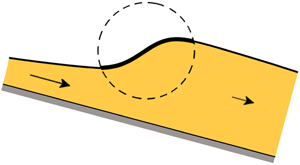
In recent years, much effort has been devoted to bringing the description of granular flows on a par with the well-established theory of hydrodynamics. Flowing granular matter behaves as a fluid with special properties and often admits a continuum hydrodynamic-like description. Indeed, many of the phenomena known from water have their counterpart in the flow of granular materials. One of the most spectacular examples is that of the hydraulic jump.
Stationary granular jumps, just like those in water, occur when a supercritical (fast) granular flow turns subcritical. Or in other words, when the Froude number
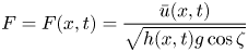 \begin{equation} F=F(x,t)=\frac{\bar{u}(x,t)}{ \sqrt{ h(x,t) g \cos \zeta} } \end{equation}
falls below the critical value  $1$. This transition reveals itself in practice by a marked increase in the thickness of the flowing sheet, see figure 1. Here $h(x,t)$ and $\bar {u}(x,t)$ denote the height of the sheet and its depth-averaged velocity, respectively, $g=9.81 \ \textrm {m}\ \textrm {s}^{-2}$ is the gravitational acceleration and $\zeta$ is the inclination angle of the chute.

Figure 1. Schematic view of a granular jump on a tilted chute, i.e. the transition zone of length  $L$ from a shallow supercritical flow (Froude number $F>1$) to a thicker subcritical one ( $F<1$). For shallow granular flows, the jump is aptly described by the height profile $h(x)$ and the depth-averaged velocity $\bar {u}(x)$, governed by the granular Saint–Venant equations (2.1) and (2.2). The jump connects two gradually varied flow regimes. In fact, the non-constancy of $h(x)$ on either side of the jump is essential for the stability of the profile.
Granular jumps are of immense importance from a practical point of view. One encounters them in snow and rock avalanches, where they may be triggered by natural obstacles or man-made flow retention structures, or by a sudden decrease in the inclination angle of the mountainside. They are ubiquitous also in agricultural and industrial applications, whenever granular materials are transported along chutes and similar devices.
During the past decades, granular jumps have become the subject of numerous studies. Pioneering work was done by Savage (Reference Savage1979) and Brennen, Sieck & Paslaski (Reference Brennen, Sieck and Paslaski1983), who undertook to derive a granular counterpart for the Bélanger equation relating the heights before and after the jump. This work initiated a surge of subsequent publications in which a variety of related granular flow phenomena were investigated, including upstream travelling bores (Gray & Hutter Reference Gray and Hutter1997; Gray, Tai & Noelle Reference Gray, Tai and Noelle2003), oblique jumps (Gray et al. Reference Gray, Tai and Noelle2003; Hákonardóttir & Hogg Reference Hákonardóttir and Hogg2005; Gray & Cui Reference Gray and Cui2007), the granular counterpart of the circular hydraulic jump known from the kitchen sink (Boudet et al. Reference Boudet, Amarouchene, Bonnier and Kellay2007), granular jets impacting on an inclined plane generating jumps in the form of teardrops and other closed shapes (Johnson & Gray Reference Johnson and Gray2011), and granular jumps on chutes with a basal topography (Viroulet et al. Reference Viroulet, Baker, Edwards, Johnson, Gjaltema, Clavel and Gray2017). Recently, Faug, Einav and their co-workers have ventured also into the regime of accelerated granular flows, exploring a wide range of stationary and non-stationary jumps (Faug Reference Faug2015; Faug et al. Reference Faug, Childs, Wyburn and Einav2015; Méjean, Faug & Einav Reference Méjean, Faug and Einav2017; Méjean et al. Reference Méjean, Guillard, Faug and Einav2020).
Mathematically, the above studies follow the classic Bélanger approach, in which one first determines the gradually varying height profiles of the super- and subcritical regimes, respectively, from the granular analogue of the so-called ‘backwater equation’ (Rouse Reference Rouse1946; Viroulet et al. Reference Viroulet, Baker, Edwards, Johnson, Gjaltema, Clavel and Gray2017). Subsequently, the mass conservation and momentum balance in macroscopic algebraic form (known as the Rankine–Hugoniot shock relations) are solved to determine the ratio of the heights before and after the jump; this then specifies the exact point where the super- and subcritical regimes must be connected by means of a vertical segment, i.e. with zero spatial extent. The state of the art in this direction has advanced as far as to augment the original analysis by the inclusion of the effects induced by the inclination of the chute (such as a gravity component) and the friction of the granular sheet with the floor of the channel (Méjean et al. Reference Méjean, Faug and Einav2017). The drawback of this approach, however, is that it does not capture the internal structure of the jump.
Savage (Reference Savage1979), in order to account for the non-zero spatial extent of this structure, approximated the jump by a linear height profile connecting the super- and subcritical regimes. Indeed, if one follows the above methodology, the structure of the jump can only be introduced independently in a heuristic way.
In the present paper, we adopt a different approach based on the mass and momentum balance in their differential form, cf. (2.1) and (2.2). Thanks to the fact that the momentum balance contains a diffusive term accounting for the normal stresses (which prevents the slope from becoming infinitely steep), this yields profiles that connect the super- and subcritical regimes in a continuous way. As a result, we are in a position to give an analytical expression for the length of the granular jump in terms of the system parameters, valid throughout the parameter space except for a few singular cases. This length, apart from being one of the characteristic features of the jump, is also one of the central ingredients of the generalized Bélanger relation proposed in recent years (Faug et al. Reference Faug, Childs, Wyburn and Einav2015; Méjean et al. Reference Méjean, Faug and Einav2017), which up to now had to be determined empirically via experiments or numerically.
The paper is organized as follows. In § 2 we present the Saint–Venant equations governing incompressible shallow granular flows, i.e. the mass and momentum balances augmented by the constitutive relations for the friction with the chute and the viscous-like force caused by the in-plane stresses. It is argued that these equations provide an appropriate framework for analysing the so-called ‘laminar’ jumps, which do not exhibit recirculation zones and for which density variations are negligible. In § 3 we focus upon the stationary wave solutions of the granular Saint–Venant equations, thereby suppressing the time-dependence and turning them into ordinary differential equations (ODEs). This paves the way for the formulation of a dynamical system, consisting of two coupled first-order ODEs. The trajectories in the phase space of this dynamical system are then exploited to unravel the internal structure of the granular jump. In fact, we find four qualitatively different types of granular jumps, summed up in figure 5. Next, in § 4, we give an analytic expression for the length of the jump in terms of the system parameters, and we discuss the range of its validity. The paper concludes in § 5, where we recapitulate our main findings and comment upon the stability of the jump profiles.
2. The governing equations
2.1. Mass and momentum balance
For our purposes, the behaviour of a flowing granular sheet is conveniently described in terms of its height  $h(x,t)$ and depth-averaged velocity $\bar {u}(x,t)$. The latter is defined as $\bar {u}(x,t) = \int _{0}^{h(x,t)} u(x,z,t) \,\textrm {d}z / h(x,t)$, where $u(x,z,t)$ is the detailed velocity profile depending on the depth $z$. Flow variations in the cross-wise direction are ignored, hence both $h(x,t)$ and $\bar {u}(x,t)$ depend only on $x$ and $t$, cf. figure 1. This is a good approximation for the laminar jumps studied in the present paper, yet by adopting this one-dimensional view one leaves aside any secondary cross-wise flow patterns, such as the convective motion induced by the boundaries of the chute or the aforementioned recirculation zones in the jump region (Brodu, Richard & Delannay Reference Brodu, Richard and Delannay2013; Faug et al. Reference Faug, Childs, Wyburn and Einav2015).
Furthermore, we treat the granular sheet as an incompressible fluid (Savage Reference Savage1979). This is a suitable approximation for the jumps we are interested in, although it must be mentioned that in reality there is a small but noticeable density increase across the jump (Faug et al. Reference Faug, Childs, Wyburn and Einav2015; Méjean et al. Reference Méjean, Guillard, Faug and Einav2020). For large Froude numbers of the incoming flow, this density increase becomes quite pronounced, in which case the assumption of incompressibility fails, but this lies beyond the laminar regime discussed here.
The pressure within the sheet is assumed to grow linearly with depth, which is called ‘lithostatic’ pressure in analogy to the well-known hydrostatic pressure for water. This is a good approximation for sufficiently shallow granular flows for which saturation effects in the pressure may be neglected (Duran Reference Duran2000; Gray & Edwards Reference Gray and Edwards2014).
The two quantities  $h(x,t)$ and $\bar {u}(x,t)$ are governed by a system of two coupled partial differential equations (PDEs), namely the mass conservation
 \begin{equation} h_t + (h \bar{u})_x = 0, \end{equation}
and the momentum balance (Gray & Edwards Reference Gray and Edwards2014; Razis et al. Reference Razis, Edwards, Gray and van der Weele2014)
 \begin{equation} (h \bar{u})_t + (h \bar{u}^2)_x = gh\sin\zeta - \mu(h, \bar{u})gh \cos\zeta - ({{\tfrac{1}{2}}}gh^2\cos\zeta )_x + \nu(\zeta) (h^{3/2} \bar{u}_x)_x, \end{equation}
where we have chosen to work with dimensional quantities in order to make our results directly comparable with previous studies on granular chute flow. In the remainder of this paper, however, we generally group the parameters in such a way that the relevant dimensionless numbers (Froude, Reynolds and  $\zeta$) show up.
The four terms featuring on the right-hand side of (2.2) represent the forces that act on the sheet: (i) the gravity component along the  $x$-direction; (ii) the adverse force stemming from the friction with the chute bed, modelled as a (height- and velocity-dependent) friction coefficient $\mu (h,\bar {u})$ multiplied by the normal reaction force acting on the granular sheet (Pouliquen Reference Pouliquen1999); (iii) the force resulting from variations in $h(x,t)$, i.e. the negative gradient of the depth-averaged pressure; (iv) the viscous-like diffusive term arising from depth-averaging the in-plane stresses in the sheet (Gray & Edwards Reference Gray and Edwards2014).
The last of these is the granular analogue of  $\nu (h\bar {u}_x)_x$ used for water (Kranenburg Reference Kranenburg1992; Balmforth & Mandre Reference Balmforth and Mandre2004), which proved to be an essential extension of the shallow water equations, preventing the profile from becoming non-smooth, keeping its slope everywhere finite. Also in granular flows the diffusive term plays a similar role. It always remains very small compared to the other terms in the momentum balance (Razis, Kanellopoulos & van der Weele Reference Razis, Kanellopoulos and van der Weele2018), yet its contribution is crucial for two reasons: (a) It comes into action when there are variations in $\bar {u}(x,t)$ (implying also variations in $h(x,t)$), flattening them out and averting the build-up of discontinuities. (b) Being the only term in the equation of motion that involves a second-order derivative, it adds a second dimension to the phase space of the associated dynamical system (see § 3), thus paving the way for a host of two-dimensional structures – e.g. spiral points or Hopf bifurcations (Razis, Kanellopoulos & van der Weele Reference Razis, Kanellopoulos and van der Weele2019) – that were not possible in the one-dimensional phase space of the inviscid theory. We note that our results do not depend critically on the exact form of the viscous-like term. It is simply too small for that; other versions may be anticipated to produce qualitatively similar jumps as long as they represent a diffusive force (i.e. featuring a second-order spatial derivative).
2.2. Constitutive relations
The above equations (2.1) and (2.2) must be supplemented by constitutive relations for  $\mu (h,\bar {u})$ and $\nu (\zeta )$. For the friction coefficient $\mu (h,\bar {u})$ we use the expression first introduced by Pouliquen (Reference Pouliquen1999), which gives an accurate description as long as the granular sheet is fully dynamic and does not exhibit stopping regions (Pouliquen & Forterre Reference Pouliquen and Forterre2002; Edwards & Gray Reference Edwards and Gray2015):
 \begin{equation} \mu(h,\bar u) = \mu_1 + \frac{\mu_2 - \mu_1}{1 + K_s \sqrt{g\cos\zeta}\,h^{3/2}\,\bar{u}^{-1}}. \end{equation}
Recent studies (Edwards et al. Reference Edwards, Viroulet, Kokelaar and Gray2017, Reference Edwards, Russell, Johnson and Gray2019) have enriched this friction law by an offset in the Froude number  $F=\bar {u}/\sqrt {h g \cos \zeta }$ appearing in (2.3), yet for smooth glass beads the offset is zero (Russell et al. Reference Russell, Johnson, Edwards, Viroulet, Rocha and Gray2019), so for an experimental verification of our results we recommend using this material. In the above friction law, $\mu _{1} (= \tan \zeta _{1})$, $\mu _{2} (= \tan \zeta _{2})$ and $K_s$ are experimentally obtained parameters. In the present paper we will take $\mu _1=0.384$ (i.e. $\zeta _1=21.0^{\circ }$), $\mu _2=0.594$ ( $\zeta _2=30.7^{\circ }$) and $K_s = 209\ \textrm {m}^{-1}$. Here $\zeta _{1,2}$ denote the two inclination angles that delimit the interval in which uniform granular flows are possible. For $\zeta < \zeta _{1}$ the granular sheet remains at rest, whereas for $\zeta > \zeta _{2}$ it sweeps downwards in an accelerated fashion.
The parameter  $K_s$ is in fact a compound quantity, namely $K_s = \beta / \mathcal {L}$, denoting the ratio of the smallest value of the Froude number ( $\beta$) for which the granular sheet is still fully dynamic and the length scale $\mathcal {L}$. For $F < \beta$, stagnant regions appear (Edwards & Gray Reference Edwards and Gray2015); the present study focuses on flows with $F > \beta$ throughout, for which the granular sheet is everywhere in motion. For recent work on the non-dynamic regime, featuring a generalized friction law, see Edwards et al. (Reference Edwards, Viroulet, Kokelaar and Gray2017, Reference Edwards, Russell, Johnson and Gray2019).
The length  $\mathcal {L}$ is the thickness of the deposition layer (usually ranging from $1$ to $2$ particle diameters) that is left on the bed of a roughened chute after a uniform flow has passed over it. The precise values of $\beta$ and $\mathcal {L}$ depend on the specifics of the particles and the chute (Pouliquen & Forterre Reference Pouliquen and Forterre2002; Forterre & Pouliquen Reference Forterre and Pouliquen2003; Gray & Edwards Reference Gray and Edwards2014; Razis et al. Reference Razis, Edwards, Gray and van der Weele2014; Edwards & Gray Reference Edwards and Gray2015; Edwards et al. Reference Edwards, Viroulet, Kokelaar and Gray2017). We choose $\beta =0.136$ and $\mathcal {L} = 0.65$ mm, representing the laboratory chute of Pouliquen & Forterre (Reference Pouliquen and Forterre2002) with spherical glass beads of diameter $0.50 \pm 0.04$ mm, so that $K_s = 209\ \textrm {m}^{-1}$. Also the chosen values of the limiting angles $\zeta _1$ and $\zeta _2$ correspond to that same set-up.
For the coefficient  $\nu (\zeta )$, we adopt the expression derived on the basis of $\mu (I)$-rheology by Gray & Edwards (Reference Gray and Edwards2014):
 \begin{equation} \nu(\zeta) = \frac{2 g \sin\zeta }{9 K_s \sqrt{g \cos\zeta}}\gamma(\zeta),\quad \textrm{where}\ \gamma(\zeta) = \frac{\mu_2 - \tan\zeta}{\tan\zeta - \mu_1}. \end{equation}
It should be noted that this parameter  $\nu (\zeta )$ has dimensionality $\textrm {m}^{3/2} \ \textrm {s}^{-1}$, which differs from the dimensions $\textrm {m}^{2}\ \textrm {s}^{-1}$ of the familiar viscosity coefficient of fluid dynamics. So the granular term $\nu (\zeta ) (h^{3/2} \bar {u}_x)_x$ as a whole is viscous-like, yet its composition is fundamentally different from that of the analogous term for standard fluids. For a detailed discussion of the origins and interpretation of the expression (2.4) we refer to Gray & Edwards (Reference Gray and Edwards2014) and Razis et al. (Reference Razis, Edwards, Gray and van der Weele2014). Here we restrict ourselves to noting that the coefficient $\nu (\zeta )$ is positive (and hence represents a positive diffusive force, smoothing the profile) in the interval $\zeta _1 < \zeta < \zeta _2$, decreasing monotonically from infinity at $\zeta =\zeta _1$ to zero at $\zeta =\zeta _2$. Outside this interval, (2.4) gives a negative value and loses its validity; this is a consequence of the ill-posedness of the $\mu (I)$-rheology in these regions (Gray & Edwards Reference Gray and Edwards2014).
In closing this section on the governing equations, let us briefly discuss an elementary yet important solution to (2.1) and (2.2), namely steady uniform flow. In this case, the sheet has a uniform thickness  $h_n$ (known as the natural height in open channel hydraulics) and flows at constant velocity $\bar {u}_n$. All derivatives with respect to $x$ and $t$ then vanish, so (2.1) is satisfied trivially. In (2.2) the only terms that survive are those of gravity and friction, which must therefore precisely balance each other: $\tan \zeta = \mu (h,\bar {u})$. Using the friction law (2.3), this yields the following relation between the velocity and the thickness of a uniformly flowing sheet:
 \begin{equation} \bar{u}_n = \frac{ K_s \sqrt{g \cos \zeta}}{ \gamma(\zeta)}~h_{n}^{3/2}, \end{equation}
known as the depth-averaged Bagnold velocity law (Bagnold Reference Bagnold1966; Duran Reference Duran2000).
3. The dynamical systems approach
3.1. Granular jumps as stationary waveforms
The granular jumps we are interested in are stationary waveforms, meaning that their height and depth-averaged velocity do not depend on time. With  $h=h(x)$ and $\bar {u}=\bar {u}(x)$, the governing equations (2.1) and (2.2) become ODEs. The first one reduces to $(h\bar {u})' = 0$, with the prime denoting differentiation with respect to $x$, and can readily be integrated to give
 \begin{equation} h\bar{u} = Q. \end{equation}
The integration constant  $Q$ is the flux of material per unit width. With $\bar {u}(x) = Q/h(x)$, and hence $\bar {u}' = -Qh^{-2}h'$ and $\bar {u}''=-Q(h^{-2} h''-2h^{-3}(h')^2)$, the momentum balance (2.2) takes the form of a nonlinear second-order ODE for $h(x)$:
 \begin{equation} \frac{\nu }{Q } h^{3/2}h'' -\frac{\nu}{2 Q }h^{1/2}(h')^2 + \left( \frac{h^3}{h_c^3} -1 \right) h' - \left( \tan\zeta - \mu(h) \right) \frac{h^3}{h_c^3} =0, \end{equation}
where, thanks to the substitution  $\bar {u} = Q h^{-1}$, the friction coefficient $\mu (h,\bar {u})$ has now also become a function of $h$ alone:
 \begin{equation} \mu(h) = \mu_1 + \frac{\mu_2 - \mu_1}{1 + \gamma(\zeta)(h/h_n)^{5/2} }. \end{equation}
Here  $h_c$ denotes the critical height for which the Froude number equals $1$, and $h_n$ is the uniform flow height from (2.5), known in hydraulics as the natural height:
 \begin{equation} h_c = \left( \frac{Q^2}{g \cos\zeta} \right)^{1/3}, \quad h_n=\left( \frac{Q \gamma(\zeta)}{K_s \sqrt{g \cos\zeta}} \right)^{2/5}. \end{equation}
The former follows from the definition of the Froude number (1.1) by substituting  $\bar {u}=Q/h$ and setting $F=1$. The latter is found from (2.5) with $\bar {u}_n = Q/h_n$.
It may be noted that the coefficients in (3.2) have been grouped in such a way that all terms are dimensionless. In particular, the combination  $Q/ (\nu h^{1/2})$ is the granular Reynolds number, and $(h_c/h)^{3/2}$ is the Froude number. We will come back to these numbers in the context of (3.12a,b).
In analogy with the standard theory of open channel flow, one may use the quotient  $h_c/h_n$ to characterize granular chutes as being (i) mild if $h_c < h_n$, (ii) critical if $h_c = h_n$, or (iii) steep if $h_c > h_n$. This is illustrated in figure 2. For the critical case, $h_c = h_n = \gamma (\zeta _{*})/K_s$, while the corresponding value of $\zeta _{*}$ is determined by $\gamma ^3(\zeta _{*}) \cos \zeta _{*} = Q^2 K_s^3/g$. The channel is mild/steep for inclination angles that are smaller/larger than $\zeta _{*}$, cf. figure 2(a).
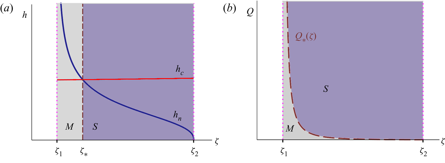
Figure 2. (a) The heights  $h_c$ and $h_n$ vs. $\zeta$ defined by (3.4a,b) at a given fixed value of $Q$. For inclination angles $\zeta _1 < \zeta < \zeta _{*}$ the chute is termed mild ( $M$), whereas for $\zeta _{*}<\zeta <\zeta _2$ it is termed steep ( $S$). The vertical dashed line marks the border between the regimes $M$ and $S$. (b) The mild and steep regimes in the $(\zeta ,Q)$ parameter diagram, separated by the dashed curve $Q_{*}(\zeta )$ of (3.5). Plot (a) represents a horizontal sweep through plot (b).
Alternatively, one can hold the angle  $\zeta$ constant and change the value of $Q$ (by tuning the inflow of material at the top of the chute). Then the chute is critical for
 \begin{equation} Q_{*}(\zeta) = \sqrt{\frac{g}{K_s^3} \gamma^3(\zeta) \cos\zeta}, \end{equation}
while it is mild/steep for  $Q$ smaller/larger than $Q_{*}(\zeta )$. Equation (3.5) defines the critical line separating the mild and steep regimes, depicted by the dashed curve in the $(\zeta ,Q)$ parameter diagram of figure 2(b).
The first two terms in (3.2) are due to the viscous-like (diffusive) term  $\nu (h^{3/2} \bar u_x)_x$ in the momentum balance (2.2). In the absence of these terms, i.e. in the inviscid limit $\nu = 0$, we would be left with a first-order ODE, namely the granular counterpart of the classic ‘backwater equation’ of open channel hydraulics (Chanson Reference Chanson2009). The backwater equation predicts the gradually varying profiles of the granular sheet before and after the jump, yet it is unable to capture the jump itself, which must then be represented by a vertical segment (satisfying the Rankine–Hugoniot shock relations) linking the two aforementioned profiles. As noted in § 1, this is the standard way of dealing with hydraulic and granular jumps to date (Gray & Cui Reference Gray and Cui2007; Johnson & Gray Reference Johnson and Gray2011; Faug et al. Reference Faug, Childs, Wyburn and Einav2015; Viroulet et al. Reference Viroulet, Baker, Edwards, Johnson, Gjaltema, Clavel and Gray2017; Méjean et al. Reference Méjean, Faug and Einav2017, Reference Méjean, Guillard, Faug and Einav2020). The central point of the present paper is that we go beyond this: we show how stationary jumps naturally arise as continuous solutions of the viscous equation (3.2).
3.2. The dynamical system governing granular jumps
The second-order ODE (3.2) can be cast in the form of two coupled first-order ODEs (i.e. a dynamical system) as follows:
 \begin{gather} h' = s \equiv f_1(s), \end{gather}
 \begin{gather}s' = \frac{s^2}{2h } - \frac{Q }{\nu h_c^3} \frac{\left( h^3 - h_c^3 \right) s }{ h^{3/2}} + \frac{Q }{\nu h_c^3}\left( \tan\zeta - \mu(h) \right) h^{3/2} \equiv f_2(h,s), \end{gather}
where the symbol  $s$ has been chosen to denote the slope $h'(x)$ of the height profile.
Fixed points of the above system are found by setting (3.6a) and (3.6b) equal to zero simultaneously, i.e.  $f_1(s)= s = 0$ and $f_2(h,s)=0$. The first of these gives $s=0$, implying that any fixed point corresponds to a flat region of the flow.
Substituting  $s=0$ into (3.6b), one finds $\tan \zeta = \mu (h)$, i.e. the previously mentioned balance between gravity and friction that characterizes a uniform flow (in accordance with the companion condition $s=0$). With $\mu (h)$ as in (3.3), this balance takes the form
 \begin{equation} \tan\zeta = \mu_1 + \frac{\mu_2 - \mu_1}{1 + \gamma(\zeta)(h/h_n)^{5/2} }, \end{equation}
which can be rewritten as
 \begin{equation} \gamma(\zeta)(h/h_n)^{5/2} = \frac{\mu_2 - \tan\zeta}{\tan\zeta -\mu_1} \left(= \gamma(\zeta) \right), \end{equation}
where in the last, bracketed step we have used the definition of  $\gamma (\zeta )$ from (2.4). Now, unless $\gamma (\zeta )$ is zero or infinite, this immediately leads to the conclusion that $h/h_n = 1$. Thus, in the interval of interest $\zeta _1 < \zeta < \zeta _2$, where $\gamma (\zeta )$ is finite, we find that the dynamical system has a single real fixed point $(h,s) = (h_n,0)$.
The value of  $h_n$ varies between two limiting cases: (i) for $\zeta _1$ the value of $\gamma (\zeta )$ diverges and we find from (3.4a,b) that $h_n(\zeta _1) \rightarrow \infty$ (i.e. a sheet of unbounded thickness), whereas (ii) for $\zeta _2$ we have $\gamma (\zeta _2)=0$ and $h_n(\zeta _2) = 0$, which represents an empty chute. Figure 2(a) shows how the natural thickness $h_n$ decreases as a function of $\zeta$.
A linear stability analysis of the fixed point  $(h_n,0)$ shows that it is a saddle, i.e. the two eigenvalues of the Jacobian matrix are real and of opposite sign:
 \begin{equation} \lambda_{1,2} = \frac{1}{2} \left\{ \frac{\partial f_2}{\partial s} \pm \sqrt{ \left( \frac{\partial f_2}{\partial s} \right)^2 + 4 \frac{\partial f_2}{\partial h} } \right\}, \end{equation}
with  $f_2(h,s)$ as defined in (3.6b). These eigenvalues $\lambda _{1,2}$ are given with the understanding that the index $1$ corresponds to the plus sign, and $2$ to the minus sign, and that all derivatives are evaluated at the fixed point $(h,s) = (h_n,0)$:
 \begin{equation} \left.\frac{\partial f_2}{\partial h} \right|_{(h_n,0)} = \frac{5}{2} \frac{(\mu_2-\mu_1) \gamma Q h_n^{1/2}}{(1+\gamma)^2\nu h_c^3 } ,\quad \left.\frac{\partial f_2}{\partial s}\right|_{(h_n,0)} = -\frac{Q }{\nu h_n^{3/2}}\left(\frac{h_n^3}{h_c^3}-1 \right). \end{equation}
The eigenvalues will play a central role in § 4 where we study the length of the jump. Here we note that  $\lambda _1 > 0 > \lambda _2$, with $\lambda _2$ being larger in absolute value than $\lambda _1$ for mild channels, and vice versa for steep channels.
We now turn to the nullclines of the system (3.6a) and (3.6b), given by  $h'=0$ and $s'=0$, respectively. Evidently, the fixed point $(h_n,0)$ lies at the intersection of the two nullclines. The nullclines play a crucial role in the analysis of the jumps because they govern the asymptotic behavior of the trajectories in phase space, as evidenced in figure 3. That is to say, they determine the gradually varying profiles before and after the jump.
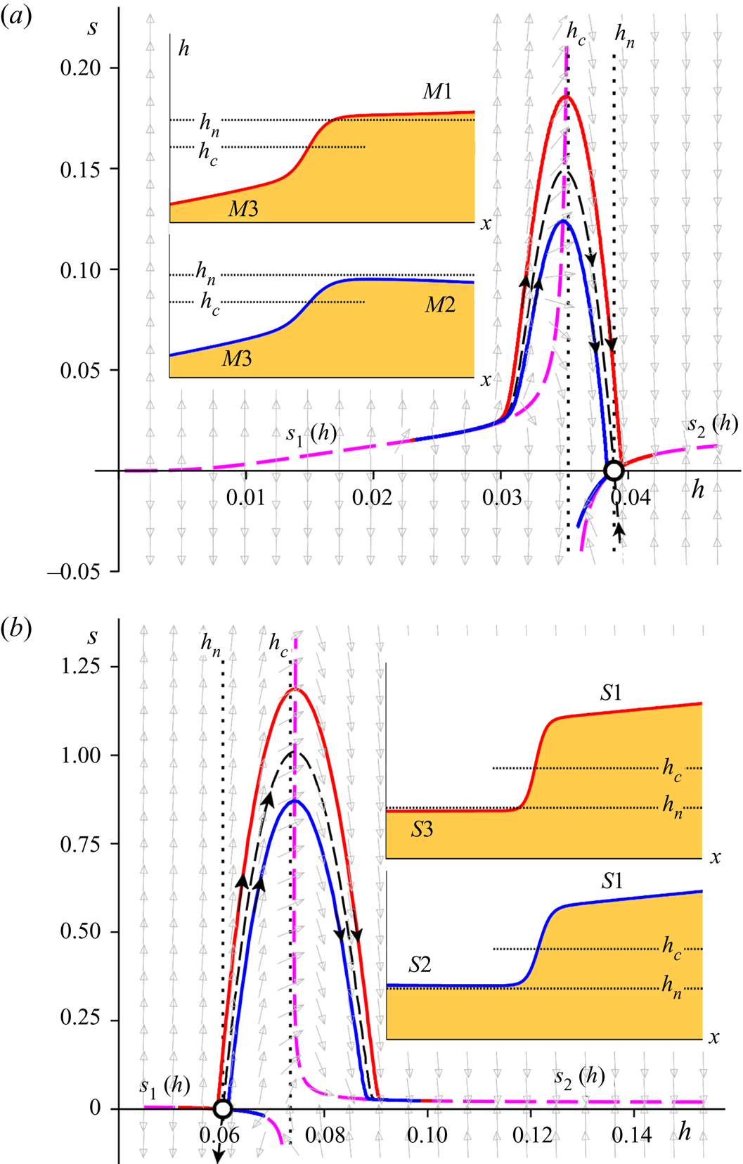
Figure 3. Phase portraits of the dynamical system (3.6a) and (3.6b) for mild (a) and steep (b) chutes, which are seen to be each other's mirror image. The dashed thick curves (magenta) designate the nullcline (3.11), governing the asymptotic behavior for small and large  $h$. The solid red and blue curves represent the two types of jumps occurring on each chute; the jump region always manifests itself as a near-parabolic orbit following the ‘backbone curve’ formed by the stable/unstable manifold of the saddle, indicated by the thin black dashed line. The remaining manifolds of the saddle (unstable and stable, respectively) are locally tangent to the nullclines $s_2(h)$ and $s_1(h)$. (a) Mild: The curves travel together in the supercritical regime and then go their separate ways; the associated profiles $h(x)$ (see insets) are the jumps $M3 \rightarrow M1$ and $M3 \rightarrow M2$. (b) Steep: Here the curves start out differently and come together in the subcritical regime; the profiles $h(x)$ (insets) are the jumps $S3 \rightarrow S1$ and $S2 \rightarrow S1$. The dotted lines indicate the levels $h_c$ and $h_n$, and the grey arrows in the background show the direction field. The length scales $h$ and $x$ are expressed in metres; the slope $s =\textrm {d}h/{\textrm {d} x}$ is dimensionless. Parameter values: $\zeta = 22.0^{\circ {}}$, $Q=0.02\ \textrm {m}^2\ \textrm {s}^{-1}$ (mild) and $Q=0.06\ \textrm {m}^2\ \textrm {s}^{-1}$ (steep).
The nullclines are given by: (i)  $f_1(s)=s=0$, i.e. simply the horizontal axis in the phase space, and (ii) $f_2(h,s)=0$, which has a more intricate shape, depicted by the thick dashed curves in figure 3(a,b). Since $f_2(h,s)=0$ is a quadratic equation in $s$, it can be solved explicitly to yield
 \begin{equation} s_{1,2}(h) = ~\frac{Q }{\nu h^{1/2}} \left\{ \frac{h^3}{h_c^3} -1 \pm \sqrt{\left(\frac{h^3}{h_c^3}-1\right)^2 - 2 \frac{\nu h^{1/2}}{Q} \frac{h^3}{h_c^3} (\tan\zeta - \mu(h))} \right\}, \end{equation}
where we have collected all quantities involved in dimensionless groups, among which one may recognize the Reynolds number (as defined for granular chute flow by Gray & Edwards (Reference Gray and Edwards2014), featuring the coefficient  $\nu (\zeta )$ from the viscous-like term) and the Froude number. Indeed, for the stationary wave profiles considered here, these dimensionless numbers are given by
 \begin{align} R=R(h)= \frac{\bar{u} \sqrt{h}}{\nu} = \frac{Q}{ \nu h^{1/2}},\quad F = F(h)= \frac{\bar{u}}{\sqrt{h g \cos\zeta}} = \frac{Q }{\sqrt{h^3 g \cos\zeta} } = \left( \frac{h_c}{h} \right)^{3/2}. \end{align}
 The nullcline  $s_{1,2}(h)$ given by (3.11) consists of two branches, the asymptotic behaviour of which is especially relevant for the jump profile as a whole. For small $h$, i.e. in the extreme supercritical regime, the behaviour of the nullcline (3.11) may be inferred from its series expansion around $h=0$:
 \begin{align} s_1(h) = (\mu_2-\tan\zeta) \left[ \frac{h^3}{h_c^3} \left( 1 \!+ \frac{\gamma^2(\zeta) }{1\!+\gamma(\zeta)} \frac{h^{5/2}}{h_n^{5/2}} \right) + \frac{h^6}{h_c^6} \left( 1+ (\mu_2-\tan\zeta) \frac{ \nu h^{1/2}}{2Q} \right) \right] \!+ O(h^8), \end{align}
where  $\mu _2$ features prominently because $\lim _{h\rightarrow 0} \mu (h) = \mu _2$. The dimensionless groups of the Froude and Reynolds numbers are also apparent in (3.13). The fact that the leading term is of order $h^3$ explains the almost horizontal departure from $s_1(0) = 0$ of the associated dashed line in figure 3(a).
At the other end, i.e. in the extreme subcritical regime for large  $h$, the nullcline attains a constant value,
 \begin{equation} \lim_{h \rightarrow \infty} s_2(h) = \tan\zeta - \mu_1, \end{equation}
which corresponds to a linearly increasing height profile  $h(x)$. It is not horizontal with respect to the laboratory, as is the case for hydraulic jumps in water, but tilted downward with respect to this horizontal with an offset angle $\zeta _1$. This offset was first observed experimentally by Faug et al. (Reference Faug, Childs, Wyburn and Einav2015).
Figure 3(a) gives a detailed view of granular jumps in a mild chute. For small values of  $h$, where the flow is supercritical, the trajectories run close to the nullcline $s_{1}(h)$ of (3.11). Then they depart from it and start to follow a near-parabolic path, whose shape is dictated by the stable manifold of the saddle point. Indeed, this manifold serves as a ‘backbone’ around which all jump trajectories are organized, following the local direction field. Close to the top of the orbit they cross the critical value $h_c$, where the Froude number $F=(h_c/h)^{3/2}$ drops below $1$, and the flow becomes subcritical. Subsequently, the trajectories descend to the neighbourhood of the saddle $(h_n,0)$ and turn either right or left (or, in the borderline case, land exactly upon the saddle).
The red trajectory in figure 3(a) turns right and connects to the rightmost branch  $s_{2}(h)$ of the nullcline, forming the profile $M1$; here we adopt the standard nomenclature for open channel flow, where one distinguishes three gradually varied profiles $M1$,
$M1$,  $M2$ and $M3$ for hydraulically mild channels and, likewise, three gradually varied profiles $S1$,
$S1$,  $S2$ and $S3$ for steep channels (Rouse Reference Rouse1946; Le Méhauté Reference Le Méhauté1976). The granular profile $M1$ eventually attains the constant slope $s = \tan \zeta - \mu _1$. As mentioned above, for water the offset is zero and the asymptotic slope attained for large $h$ is simply $\tan \zeta$, corresponding to a free surface parallel to the horizon. This situation is met when the flow encounters a wall or a sluice gate. The same is true for granular flows: the jump $M3 \rightarrow M1$ (now with the offset) typically occurs between two sluice gates, the first of which may simply be the inlet at the top of the chute.
The blue trajectory of figure 3(a) bends off to the left of the saddle, i.e. it goes to smaller values of  $h$ with negative slope $s$. This constitutes a qualitatively different jump, ending with the profile $M2$ instead of $M1$. In contrast to $M1$, the profile $M2$ loses height continually, and at some point may be anticipated to drop below the level $h_c$ and become supercritical again. Since the profile $M2$ is typically found for chutes ending in a fall without any hindrances, this opens up the possibility of having supercritical discharge conditions at the outlet of the chute. This is a novel prediction of the theory presented here, expanding the inviscid result according to which discharge always takes place in such a way that $F=1$ locally (Rouse Reference Rouse1946; Chow Reference Chow1959).
The jump trajectories and profiles for a steep chute (figure 3b) are seen to be the mirror images of those for mild ones (figure 3a), revealing the close connection that exists between these two classes of jumps. For steep chutes it is the unstable manifold of the saddle point that serves as the ‘backbone’ for the jumps. The red and blue trajectories now do not start together but rather end together, both of them converging to the rightmost branch of the nullcline  $s_{2}(h)$, i.e. the profile $S1$ with asymptotic slope $s = \tan \zeta -\mu _1$.
In between the mild and steep cases, one finds the borderline critical situation for which  $h_n = h_c$. This configuration requires a considerable amount of fine-tuning and can hardly be expected to be found in practice. For completeness, however, we illustrate it in figure 4. In accordance with the above observations, we see that the phase space trajectories connecting the two nullclines are their own mirror images. Indeed, the phase space itself exhibits a near-perfect symmetry around the level $h = h_c$.
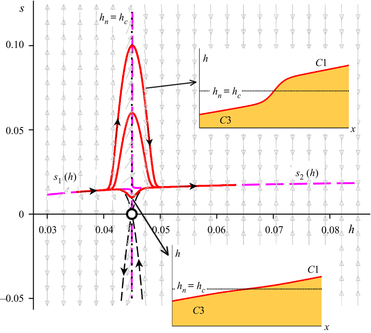
Figure 4. Phase portrait of the dynamical system (3.6a) and (3.6b) for a critical chute. Interestingly, the transition from the supercritical nullcline  $s_1(h)$ to its subcritical counterpart $s_2(h)$ can now take place in any guise ranging from an abrupt jump (upper inset) to a relatively flat interval (lower inset). The reason for this is that, in this special case, the stable and unstable manifolds of the saddle $(h_n,0)$ (denoted by the thin black dashed lines emanating from this point) do not act as backbones for the connecting trajectories. As in figure 3, $h$ and $x$ are expressed in metres, while the slope $s =\textrm {d}h/{\textrm {d} x}$ is dimensionless. The parameter values are $\zeta = 22.0^{\circ {}}$, $Q=Q_{*}=0.02876\ \textrm {m}^2\ \textrm {s}^{-1}$, cf. (3.5).
The distinguishing feature of this critical case is that the connection between the supercritical branch  $s_1(h)$ and the subcritical branch $s_2(h)$ does not necessarily involve a jump. Indeed, figure 4 shows that it can just as well take place via a relatively flat flow region. The reason for this is that the stable and unstable manifolds of the saddle point $(h_n,0)$ do not form any pronounced loop in the upper half-plane of phase space (as they do in the mild and steep cases, where they act as backbones for the jumps) but rather connect straight away, without any detours, to $s_1(h)$ and $s_2(h)$; see the thin black curves emanating from the saddle. We also observe that, since there is no room for a gradually varied profile between $h_n$ and $h_c$ in this critical case (i.e. there is no $C2$ profile), the only branches that can contribute to the transition are $C3$ (supercritical) and $C1$ (subcritical). Hence only one type of transition is possible on a critical chute, namely $C3 \rightarrow C1$, which can, however, manifest itself as anything ranging from a vigorous jump to a nearly flat region, corresponding respectively to the hill- and valley-shaped connections of figure 4.
The above findings are summarized in figure 5, which gives an overview of the various qualitatively different jump types in the mild and steep regimes of the  $(\zeta ,Q)$ parameter diagram. This figure may be compared with the experimentally obtained diagram of Faug et al. (Reference Faug, Childs, Wyburn and Einav2015) and its numerical counterpart given by Méjean et al. (Reference Méjean, Guillard, Faug and Einav2020). Indeed, our study fully explains the earlier diagrams as far as the jumps for $\zeta < \zeta _2$ are concerned, which are termed either ‘diffuse’ or ‘laminar’ by these previous authors (Faug Reference Faug2015; Faug et al. Reference Faug, Childs, Wyburn and Einav2015; Méjean et al. Reference Méjean, Faug and Einav2017, Reference Méjean, Guillard, Faug and Einav2020).
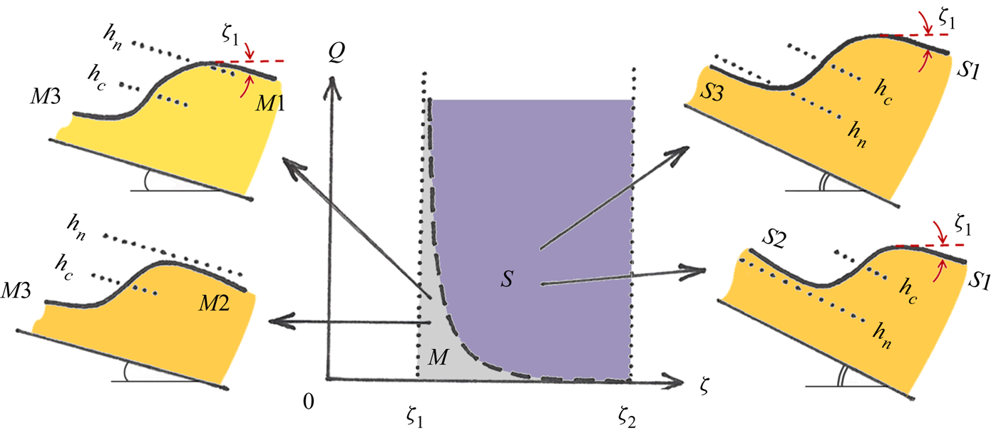
Figure 5. Overview of the four qualitatively different jump types encountered in shallow granular flow on a chute tilted at angles  $\zeta _1 < \zeta < \zeta _2$ (for which uniform flows are possible) and with varying influx $Q$. In the mild regime of the $(\zeta ,Q)$ parameter diagram one finds $M3 \rightarrow M1$ and $M3 \rightarrow M2$ (cf. figure 3a), and in the steep regime $S3 \rightarrow S1$ and $S2 \rightarrow S1$ (cf. figure 3b). The branches $M1$ and $S1$ exhibit an offset from the horizontal by an angle $\zeta _1$, experimentally detected by Faug et al. (Reference Faug, Childs, Wyburn and Einav2015) and analytically derived in (3.14). The dashed curve, $Q_{*}(\zeta )$ given by (3.5), corresponds to critical chute conditions, for which the transition ( $C3 \rightarrow C1$) does not necessarily take place via a jump, see figure 4.
The phase diagrams of the aforementioned authors also feature several types of jumps which are not accounted for in the framework of the granular Saint–Venant equations presented here. These jumps correspond to inclination angles beyond  $\zeta _2$, where the incoming flow is accelerating and would develop into an uncontrollable avalanche if it were not hindered in some way. This is done by a properly adjusted sluice gate, in front of which the granular flow organizes itself in the form of a standing jump. These jump types often exhibit ‘recirculation patterns’ and ‘internal rollers’, as well as variations in density (i.e. in the volume fraction of the particles), and belong to a different kind of flow that must be treated separately.
4. On the length of the jump
Based on the observation that the jump region in phase space manifests itself as a near-parabolic trajectory, we are able to derive an analytical approximate expression for one of the jump's most prominent features, namely its length  $L$. In the derivation that follows, we consider a granular jump on a steep chute. At the end of the section we demonstrate that a similar analysis holds for jumps on a mild chute and arrive at a unifying expression for the jump length $L$ that is valid for both regimes – apart from some well-defined cases such as the borderline situation of a critical chute.
4.1. Steep regime
In the steep regime, the near-parabolic trajectories start out from the immediate vicinity of the saddle  $(h_n,0)$ and are to a good approximation centred around the critical value $h=h_c$. As we have seen, they are organized around the unstable manifold of the saddle point, which acts as a backbone for all jumps. Here we will approximate this backbone by a parabola, which may conveniently be written as $s_{{par}}(h) = A (h-h_n) (2h_c - h_n-h)$. This form expresses the fact that the approximative parabola crosses the line $s=0$ at the points $h=h_n$ and $h=2h_c-h_n$, which are positioned symmetrically around $h=h_c$. The highest point of this parabola is $s_{{par}}(h_c) = A(h_c-h_n)^2$. The positive constant $A$ is determined from the fact that the slope of the parabola at $(h_n,0)$ should be aligned with the vector field, which here means with the saddle's unstable eigenvector. This slope is given by the positive eigenvalue, i.e. $\lambda _{1}$ of (3.9), leading to $A=\lambda _{1}/[2(h_c-h_n)]$.
This means, with  $s=\textrm {d}h/{\textrm {d} x}$, that the profile of the flow along this central parabola is described by the following first-order ODE:
 \begin{equation} \frac{\textrm{d}h}{\textrm{d} x} = A(h-h_n) (2h_c - h_n -h), \quad \textrm{with}\ A = \frac{\lambda_{1}}{2(h_c-h_n)}, \end{equation}
which can be solved analytically to yield
 \begin{equation} h_{{par}}(x)=h_c+(h_c-h_n) \tanh \left( \frac{\lambda_{1}}{2} x \right). \end{equation}
Here the integration constant has been chosen such as to satisfy the condition  $h_{{par}}(0)=h_c$, i.e. the jump corresponding to the backbone parabola is centred around the point where it crosses the critical level $h_c$. In figure 6 this reference jump, given by (4.2) and represented by the dashed curve, is compared with two profiles obtained from numerically solving the full dynamical system (3.6a) and (3.6b), denoted by the solid curves. The agreement in the jump region is very satisfactory.
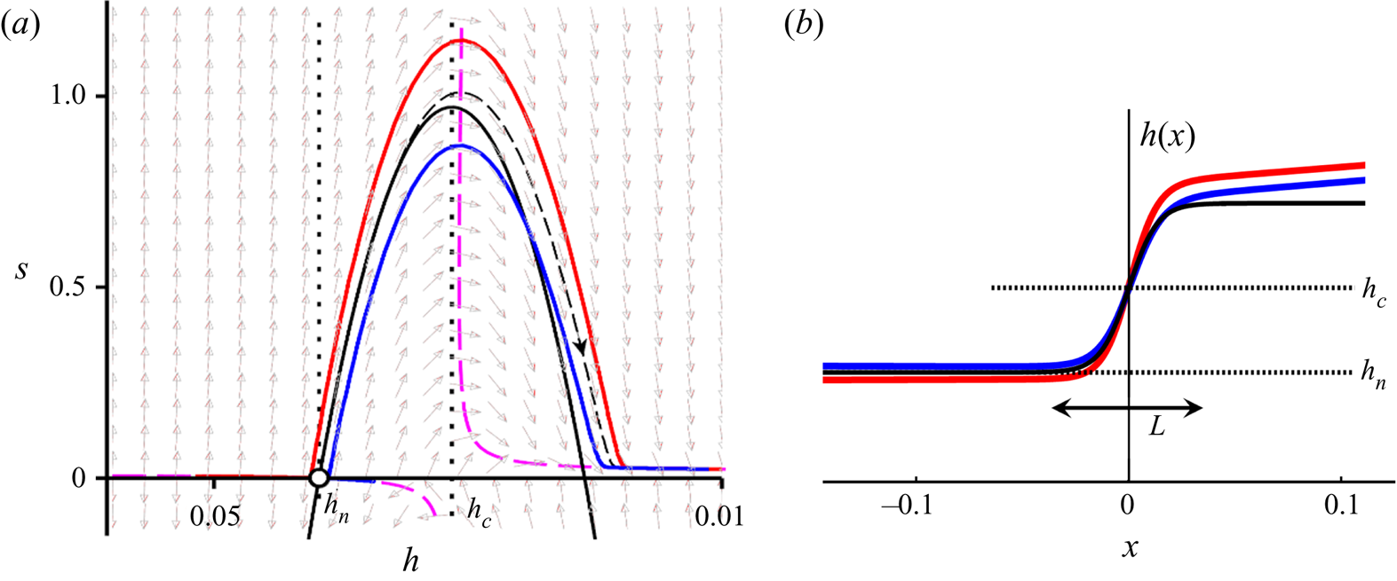
Figure 6. (a) The ‘backbone’ parabola  $s_{{par}}(h)$ in phase space (solid black curve), which in the jump region $h_n < h < (2h_c - h_n)$ approximates the unstable manifold (dashed) around which the trajectories are organized. The parameter values are the same as in figure 3(b). (b) The tanh-profile (4.2) corresponding to the backbone parabola (solid black line) together with the actual profiles $S3 \rightarrow S1$ (red) and $S2 \rightarrow S1$ (blue). The length $L$ derived from the tanh profile, given by the analytic expression (4.6), is seen to be in very good agreement with the actual extent of the jumps.
The small deviations are partly due to the fact that the red and blue trajectories do not exactly coincide with the saddle's manifold, and partly to the fact that the manifold is not precisely reproduced by the parabolic approximation. As for the first imprecision, we note that for each individual trajectory, the approximative tanh profile might be made to fit the observed jump more closely by choosing not the backbone parabola but another one that lies closer to the actual trajectory; to this end, one would select a point  $(h_p,s_p)$ on the trajectory in question and determine the coefficients $C_1$ and $C_2$ of the specific parabola $s(h)=C_1(h-h_c)^2 + C_2$ that passes through this point.
As for the second source of imprecision, it may be noted that the accuracy of reproducing the manifold in the jump region can be enhanced at will by approximating it in terms of a power series in  $(h-h_c)$, keeping any desired number of terms. Or even better, one could use a power series in $(h-h_{*})$, where $h_{*}$ denotes the height corresponding to the maximum of the manifold (which lies on the nullcline, i.e. close to but not exactly on the vertical line $h=h_c$). The gain in accuracy, however, comes at the expense of analytic elegance. The current approximation is free from numerical fitting and contains only quantities that come straight from the dynamical systems approach. Moreover, any power series with terms higher than quadratic would result in a much more intricate form than a tanh profile.
Now, the jump length  $L$ may be defined as the distance in the $x$-direction in which $h(x)$ completes $99\,\%$ of its course. Since $\tanh (\alpha x) = 0.99$ at $\alpha x = 2.65$, this gives for the reference jump: $L_S = 2 \times 2.65/ \alpha = 10.6 / \lambda _{1}$ (where the subscript $S$ serves as a reminder that we are considering a steep chute). With $\lambda _1$ given by (3.9) and (3.10a,b), this takes the form
 \begin{equation} L_S = 10.6 h_n \frac{2\nu h_n^{1/2}}{Q [1-(h_n/h_c)^3]} \left\{ 1 + \sqrt{1+10 \frac{\gamma (\mu_2-\mu_1) \nu h_n^{1/2} (h_n/h_c)^3 }{(1+\gamma)^2 Q [1-(h_n/h_c)^3]^2}} \right\}^{-1}. \end{equation}
For typical granular jumps, the quantity under the square root does not deviate significantly from  $1$ – mainly due to the smallness of the parameter $\nu (\zeta )$, which in turn can be traced back to the large value of the experimental constant $K_s$, cf. (2.4) – meaning that the value of the term in curly brackets is close to $2$. This leads to
 \begin{equation} L_S \approx 10.6 h_n \frac{\nu h_n^{1/2}}{Q [1-(h_n/h_c)^3]} = 10.6 h_n \frac{F_n^2}{R_n \left( F_n^2 -1 \right) } , \end{equation}
where  $R_n = R(h_n)$ and $F_n = F(h_n)$ denote the Reynolds and Froude numbers associated with the height $h=h_n$, cf. (3.12a,b). For the steep chutes under consideration, this is the height of the incoming supercritical flow, just upstream of the jump. In phase space the trajectories are then in the vicinity of the saddle point and are just about to commence their near-parabolic path. The analytical expression (4.4), with the parameter values used in figure 6, gives a length of $0.072$ m indicated by the double arrow in the figure; this is seen to agree very well with the spatial extent of the actual jumps (shown in red and blue).
From a dimensional point of view, it may be noted that from the system parameters one can construct a characteristic length. Given that the combination  $\nu h^{3/2} / Q$ has the dimensions of a length, an obvious candidate for such a characteristic length is $\nu h_n^{3/2} / Q$, where $h_n$ also brings in the other system parameters $g$,
$g$,  $\zeta$ and $K_s$. In this light, it stands to reason that the jump length $L_S$ given in (4.3) and (4.4) features the group $\nu h_n^{3/2} /Q$ multiplied by a non-dimensional expression.
4.2. Mild regime
Jumps on a mild chute are the mirror images of those on a steep chute. In the mild case,  $h_n > h_c$, and the near-parabolic orbits do not start in the neighbourhood of $(h_n,0)$ but end there, following the backbone formed by the stable manifold of the saddle point. This manifold can again be approximated by a parabola through $(h_n,0)$, which this time has to comply with the direction of the stable eigenvector. The slope of this vector is equal to the negative eigenvalue of the saddle, i.e. $\lambda _{2}$ of (3.9). The positive constant $A$ thus becomes $A=-\lambda _{2}/[2(h_n-h_c)]$, and the reference jump is given by $h_{{par}}(x)=h_c+(h_n-h_c) \tanh ( -\lambda _{2} x/2 )$, while the expression for its length reads $L_M = -10.6 / \lambda _{2}$ (where the subscript $M$ stands for mild). In an analogous fashion as for the steep case, this leads to
 \begin{equation} L_M \approx 10.6 h_n \frac{\nu h_n^{1/2}}{Q [(h_n/h_c)^3-1]} = 10.6 h_n \frac{F_n^2}{R_n \left( 1-F_n^2 \right) } , \end{equation}
with  $R_n$ and $F_n$ again denoting the Reynolds and Froude numbers of the flow at the height $h=h_n$. In this mild case, however, this height is found just downstream of the jump, i.e. in the subcritical regime. In phase space this occurs when the trajectories pass through the vicinity of the saddle point, where they leave their near-parabolic path and connect to the nullcline $s_2(h)$, either towards the right or to the left (for jumps of type $M3 \rightarrow M1$ or $M3 \rightarrow M2$, respectively).
4.3. A unified view
The above analysis nicely illustrates the mirror symmetry that exists between jumps on mild chutes and those on steep ones. We note that (4.4) and (4.5) can be captured in one universal equation for the jump length:
 \begin{equation} L \approx 10.6 h_n \frac{F_n^2}{R_n \mid F_n^2 -1 \mid} = 2.36 h_n \frac{\tan \zeta}{\mid F_n^2 -1 \mid}, \end{equation}
where in the last step we have used the identity  $F_n^2 / R_n = (2/9) \tan \zeta$. The Reynolds number surprisingly drops out of the final expression (4.6). This can be attributed to the fact that the parameter $\nu (\zeta )$ as defined for granular flow, (2.4), is not solely a function of the intrinsic properties of the granular material (via the factor $K_s$) but also of the external parameters $\zeta$ and $g$. It is the slope $\zeta$ that eventually survives in (4.6).
In fact, since  $h_n$ and $F_n$ depend on $\zeta$ and the flux $Q$, (4.6) can also be seen as a function of these two parameters: $L=L(\zeta ,Q)$. Contour plots of this latter function are shown in figure 7. A central role here is played by the critical curve $Q_{*}(\zeta )$, (3.5), separating the mild and steep regimes. In (4.6) this corresponds to the case $F_n = 1$, when $h_n = h_c$, for which the predicted length evidently diverges.
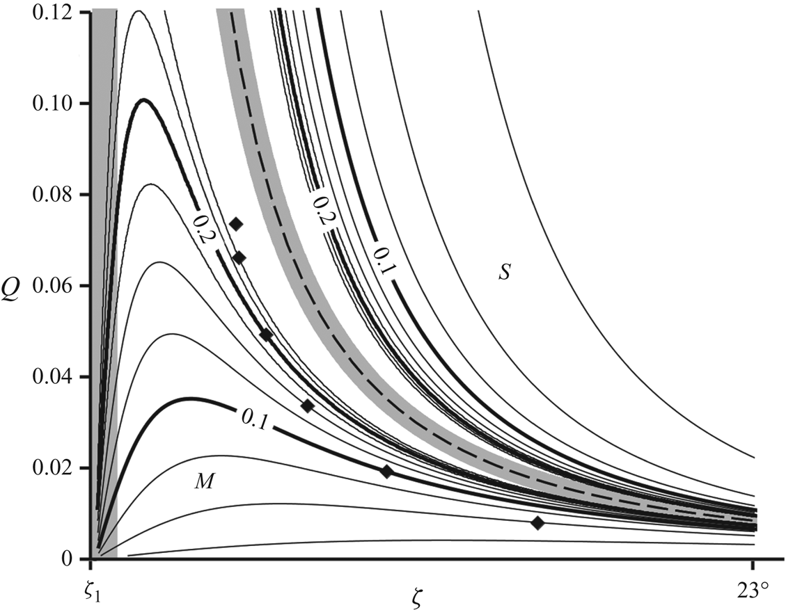
Figure 7. Contour plot of the jump length  $L(\zeta ,Q)$ predicted by (4.6) in the $(\zeta ,Q)$ parameter plane for $\zeta$ between $\zeta _1 (=21.0^{\circ })$ and $23^{\circ }$. The value of the jump length, indicated for several representative contour lines, is measured in metres. The prediction diverges on the dashed curve ( $Q_{*}(\zeta )$ given by (3.5)) separating the mild ( $M$) and steep ( $S$) regimes; as a result, (4.6) should not be used in the grey zone surrounding this critical curve. Also the vicinity of the vertical axis $\zeta =\zeta _1$ must be excluded (as indicated by the grey shading) since the parabolic approximation of the manifold in question becomes increasingly poor here. The black diamonds mark the parameter values in the mild regime for which the parabola happens to be an excellent approximation; to the left/right of these diamonds, the parabola lies above/below the manifold. In the steep regime, the parabolic approximation remains satisfactory everywhere, and the associated prediction for the jump length is accurate throughout.
As we have seen in figure 4, this borderline situation is quite different from the generic cases of mild and steep chutes, since the transition from the supercritical profile ( $C3$) to the subcritical one ( $C1$) is not dictated by the manifolds of the saddle point. As a matter of fact, the transition does not even have to take the form of a jump but can just as well occur via a very smooth flow zone linking the profiles $C3$ and $C1$. Accordingly, the length of the connecting region can assume a wide range of different values, and a different analysis would be needed to capture this singular case. (We will not pursue such an analysis here, since the critical case may be anticipated to be very rare in practice given the high amount of fine-tuning required.) In the context of figure 7, this implies that the length predicted by (4.6) – being derived on the premise that the transition takes place along the manifold – necessarily loses its validity in the neighbourhood of the critical curve $Q_{*}(\zeta )$, indicated by the grey zone surrounding it.
Away from this grey zone, the parabola is always found to give a fair approximation in the depicted steep regime ( $S$). However, in the mild regime ( $M$) things are more complicated. The parabolic approximation happens to be excellent along the line demarcated by the black diamonds in figure 7, yet it becomes less accurate as one drifts away from that line. This is not immediately translated into a loss of accuracy of the predicted length. Indeed, (4.6) proves to give satisfactory agreement with the actual lengths (obtained from solving the full dynamical system) well beyond the nominal range of validity of the parabolic approximation. One has to wander quite close to the critical curve $Q_{*}(\zeta )$ or to the vertical axis defined by the limiting angle $\zeta _1$ before the prediction fails. Both cases are shrouded by a grey zone, and both are characterized by $L(\zeta ,Q)$ diverging to infinity. In the former case, the parabola significantly undershoots the stable manifold of the saddle, while in the latter case it overshoots it by a wide margin. Here it may be noted that the limit $\zeta \rightarrow \zeta _1$ is problematic anyhow, since $\nu (\zeta )$, $\gamma (\zeta )$ and $h_n(\zeta )$ all tend to infinity at this angle.
At the other end of the phase diagram, for  $\zeta \rightarrow \zeta _2$ (not depicted in figure 7), we find $L \rightarrow 0$, just as one would expect because the parameter $\nu (\zeta )$ approaches zero here. As $\nu (\zeta )$ becomes smaller, the derivatives involved in the viscous-like term grow larger (in order to preserve the continuity of the profile), and the jump becomes very steep, reminiscent of the inviscid scenario. Before the actual limiting angle $\zeta _2$ is reached, however, the predicted jump length (4.6) becomes smaller than the grain diameter, and one should not stretch the theory beyond this point. It may be anticipated that here the jumps will cease to be laminar and that one progressively enters the regime of ‘steep colliding’ granular jumps with recirculation, as in the experiments by Faug et al. (Reference Faug, Childs, Wyburn and Einav2015), which lie outside the scope of this paper.
In summary, our results indicate that (with the exception of the grey zones and those regions where  $L$ becomes less than the size of a grain), (4.6) provides a trustworthy analytical prediction of the jump length found by solving the full dynamical system. As a next step, it would be very interesting to test this prediction experimentally. We sincerely hope that the present study may serve as a roadmap for such a future experimental survey.
5. Conclusion
In this paper we have presented granular jumps on a chute as continuous solutions of the Saint–Venant equations governing shallow granular flow. To the best of our knowledge, this is the first time that these jumps have been obtained entirely within the natural framework formed by the aforementioned equations, without resorting to additional techniques. Prior studies invariably relied on the Rankine–Hugoniot conditions across the shock zone, at the cost of concealing the internal structure of the jump. Our study has elucidated precisely this structure. To achieve this goal, the dynamical systems approach proved to be instrumental.
Indeed, in phase space the jumps manifest themselves as trajectories that leap from the supercritical branch of the nullcline to the opposite subcritical branch via a striking near-parabolic connection, see figure 3. As we have seen, the viscous-like term in the granular Saint–Venant equations is of vital importance to make this leap possible, even though the associated force always remains tiny in comparison to the other forces featuring in the momentum balance. The conspicuous near-parabolic shape of the jump region has been exploited to derive the approximate analytic expression (4.6) for the length of a typical jump (away from the grey zones in figure 7) in terms of the system parameters. It will be highly interesting to put this result to the test experimentally and investigate in a systematic manner the dependence of the jump length  $L$ on the various parameters involved. As mentioned in § 2, we recommend the use of smooth glass beads, as in the experiments by Pouliquen & Forterre (Reference Pouliquen and Forterre2002), Faug et al. (Reference Faug, Childs, Wyburn and Einav2015) and Russell et al. (Reference Russell, Johnson, Edwards, Viroulet, Rocha and Gray2019). The results of such a study may then also be compared with the numerical results of Méjean et al. (Reference Méjean, Guillard, Faug and Einav2020) on ‘laminar’ jumps. This would provide a comprehensive, three-fold approach to the problem at hand.
The phase portraits also have provided the necessary geometric perspective for revealing the mirror symmetry that exists between mild and steep granular jumps, see figure 3. This has led to a classification of the complete spectrum of jumps in fully dynamic ( $F>\beta$) shallow granular flows on a chute without hindrances and tilted at an angle $\zeta _1 < \zeta < \zeta _2$, being the realm in which uniformly flowing sheets are possible. In these flows we distinguish four different, yet intimately related types of granular jumps, which are summarized in figure 5.
The dynamical systems approach, despite the wealth of insight it provides, does not say anything about the stability of the solutions obtained. In order to settle this important issue, one must return to the original time-dependent PDEs, i.e. the granular Saint–Venant equations (2.1) and (2.2). The stability of the profiles can be demonstrated by inserting them, in perturbed form, as initial conditions into these PDEs. As an example, figure 8 shows the time evolution of a slightly perturbed profile of type  $M3 \rightarrow M1$. The perturbation (a small surplus of material in the shape of a Gaussian-like bump) is seen to generate interesting wave phenomena, which we plan to report in a future publication. In the present context, however, it suffices to note that these waves decay with time, thus confirming the stability of the jump.
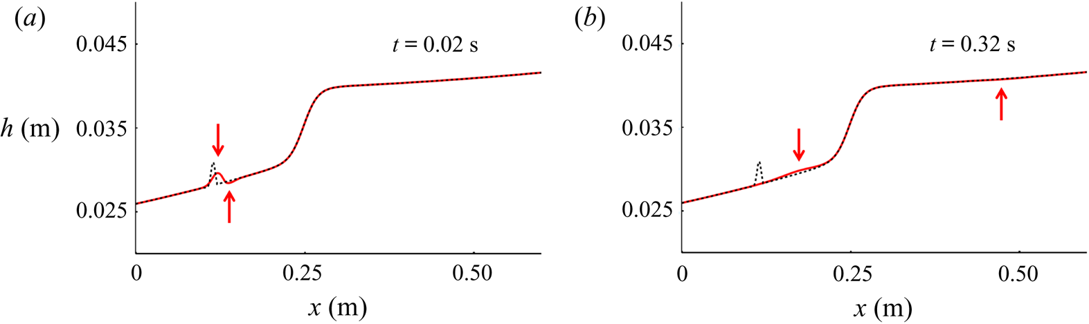
Figure 8. Stability of the granular jump  $M3 \rightarrow M1$: an initial perturbation (black dashed line) is positioned on the jump's lower, supercritical flank, and its evolution is computed from the granular Saint–Venant equations (2.1) and (2.2). The perturbation is seen to break into a dimple and a hump, which both travel to the right and decay with time, evidencing the stability of the jump. The position of the dimple is indicated by the arrow below the profile, while the hump is indicated by the arrow above it. In the second snapshot (at $t =0.32$ s) the dimple has passed the critical level $h=h_c$ and is now travelling along the upper, subcritical flank. The evolution of the system has been evaluated using the method of lines (Schiesser Reference Schiesser1991; Razis et al. Reference Razis, Kanellopoulos and van der Weele2018), with a computational space step ${\rm \Delta} x = 0.6 \times 10^{-4}$ m. The grid independence of the result has been checked by using smaller space steps.
Acknowledgements
The authors wish to thank Professor J. M. N. T. Gray (University of Manchester, UK) for introducing them to the fascinating field of granular chute flow. G. Kanellopoulos' contribution to this research is co-financed by Greece and the European Union (European Social Fund – ESF) through the Operational Programme ‘Human Resources Development, Education and Lifelong Learning’ in the context of the project ‘Reinforcement of Postdoctoral Researchers – 2nd Cycle’ (MIS-5033021), implemented by the State Scholarships Foundation (IKY).
Declaration of interests
The authors report no conflict of interest.


 Open access