


1. Introduction
Natural geological phenomena, such as the formation of laccoliths by the lateral flow of lava beneath an elastic sediment layer (Michaut Reference Michaut2011; Lister, Peng & Neufeld Reference Lister, Peng and Neufeld2013; Pihler-Puzović et al. Reference Pihler-Puzović, Juel, Peng, Lister and Heil2015) and gravity-driven surface lava flows under solidified crusts (Pihler-Puzović et al. Reference Pihler-Puzović, Juel, Peng, Lister and Heil2015), as well as human-made applications, such as hydraulic fracturing for production of oil and gas from shale formations that releases fluid waste (Dana et al. Reference Dana, Zheng, Peng, Stone, Huppert and Ramon2018), formation and growth of blisters (Pihler-Puzović et al. Reference Pihler-Puzović, Juel, Peng, Lister and Heil2015), manufacture of flexible electronics and micro-electromechanical systems, the reopening of airways, and the suppression of viscous fingering in a deformable Hele-Shaw cell (Lister et al. Reference Lister, Peng and Neufeld2013), involve viscous spreading of fluids beneath elastic surfaces.
It is known that in surface-tension-driven problems, in the limit of length scales smaller than the capillary length, an assumption that the thickness of a droplet tends to zero at the contact line leads to divergent viscous stresses, and thus to the arresting of the contact line propagation (Huh & Scriven Reference Huh and Scriven1971). This apparent paradox, which conflicts with everyday experience of spreading droplets, was resolved by considering the development of a thin precursor film due to intermolecular interactions (e.g. van der Waals) in advance of the contact line (de Gennes Reference de Gennes1985). Thus a local balance between viscous dissipation and the rate of change of surface energy gives rise to Tanner's law (Tanner Reference Tanner1979; Bonn et al. Reference Bonn, Eggers, Indekeu, Meunier and Rolley2009), in which the droplet radius advances with speed  ${\rm d}R/{\rm d}t\propto \theta ^3$ for apparent contact angle $\theta$, thus using droplet volume conservation, one obtains readily that $R$ increases as $t^{1/10}$ (de Gennes, Brochard-Wyart & Quéré Reference de Gennes, Brochard-Wyart and Quéré2004).
This approach was extended recently by employing the pre-wetting layer to study a propagation of a viscous flow between elastic plates and a rigid solid. For example, Lister et al. (Reference Lister, Peng and Neufeld2013) examined an elastic peeling problem in the distinct limits of peeling by bending and peeling by pulling, and applied their results to the radial spread of a fluid blister over a thin pre-wetting film. Pihler-Puzović et al. (Reference Pihler-Puzović, Juel, Peng, Lister and Heil2015) investigated single- and two-phase displacement flows in which the injection of fluid is accommodated by the inflation of the sheet and the outward propagation of an axisymmetric front beyond which the cell remains approximately undeformed. Peng & Lister (Reference Peng and Lister2020) investigated the spreading of viscous fluid injected under an elastic sheet, where initially the viscous liquid fills the narrow gap, and is driven by gravity and by elastic bending and tension forces, resisted by viscous forces. By identifying all of the possible asymptotic combinations, they revealed a rich variety of different behaviours. Hewitt, Balmforth & De-Bruyn (Reference Hewitt, Balmforth and De-Bruyn2015) considered a nonlinear diffusion equation describing the planar spreading of a viscous fluid injected between an elastic sheet and an underlying rigid plane, where the dynamics was assumed to depend on the physical conditions at the contact line where the sheet is lifted off the plane by the fluid. Bunger & Detournay (Reference Bunger and Detournay2007) proposed a small-time asymptotic solution for a penny-shaped fluid-driven fracture, which was obtained semi-analytically. In particular, they concluded that the similarity solution is unusual since the two length scales of the problem – the radius of the fracture and the radius of the fluid front – evolve according to two different power laws of time.
Other works concentrated on the propagation of cracks in infinite domains, in the two limits of a thin or thick elastic plate. For example, Lai et al. (Reference Lai, Zheng, Dressaire, Wexler and Stone2015) performed an experimental investigation of a fluid-driven crack in a gelatin matrix, and verified the influence of different experimental parameters such as the injection flow rate, Young's modulus of the matrix, and fluid viscosity on the shape of crack. Different governing physical mechanisms of the peeling process were also studied extensively. Considerable work was done taking into account the adhesive interaction between the solid and the fluid (McEwan & Taylor Reference McEwan and Taylor1966; Hosoi & Mahadevan Reference Hosoi and Mahadevan2004). Some studies concentrated on investigating systems with gravitation-governed peeling processes (Buckmaster Reference Buckmaster1977; Huppert Reference Huppert1982; Momoniat Reference Momoniat2006; Howell, Robinson & Stone Reference Howell, Robinson and Stone2013; Balmforth, Craster & Hewitt Reference Balmforth, Craster and Hewitt2015; Hewitt et al. Reference Hewitt, Balmforth and De-Bruyn2015).
In this work, we examine the effect of a pre-wetting layer on the rate of propagation of a viscous flow within an infinitely deep and long domain. Our model, which aims to explain fluid dynamics that occurs when a crack already exists, is commonly denoted in the context of hydraulic fracturing as ‘flowback’ or ‘produced water’ (see e.g. Dana et al. Reference Dana, Zheng, Peng, Stone, Huppert and Ramon2018). Specifically, our model problem is governed by the equations of elasticity, where the lubrication theory is used to describe the fluid dynamics in the whole region (close to the peeling front and away from it). In this sense, considerable work was done on infinite elastic spaces and half-spaces in the context of hydraulic fracturing. Various models of hydraulically driven crack propagation were suggested (Spence & Sharp Reference Spence and Sharp1985; Lister Reference Lister1990; Savitski & Detournay Reference Savitski and Detournay2002; Lai et al. Reference Lai, Zheng, Dressaire, Wexler and Stone2015, Reference Lai, Zheng, Dressaire, Ramon, Huppert and Stone2016a,Reference Lai, Zheng, Dressaire and Stoneb). Most of the analytic works implement known solutions for general axisymmetric problems of stress functions, e.g. Love's bi-harmonic equations (Sneddon Reference Sneddon1995). The integral relation between the fluid film pressure and the surface deformation, derived by Spence & Sharp (Reference Spence and Sharp1985), together with Reynolds equation obtained from the fluid analysis, completes the definition of the integro-differential problem and allows us to gain insight into the behaviour of the system under consideration. More specifically, in § 2, we present the model problem, and in § 3, we discuss the self-similarity solutions in the two limits of thick and thin pre-wetting layers, where a thin pre-wetting layer represents a precursor film. In § 4, we discuss our results, including a comparison between the solutions for the dynamic linear and nonlinear problems, and the corresponding solutions obtained by self-similarity analysis in these two limits. We conclude our findings in § 5, give the details of our numerical algorithms in the various cases in Appendix A, and present additional details and comparisons between our results and the results known from the literature in Appendix B.
2. Problem formulation
In this work, we consider the configurations that are shown in figure 1, where a fluid layer with initial thickness  $h_0$ is situated between infinitely deep and long elastic and rigid solids, or between two elastic solids. Hereafter, we will focus only on the configuration shown in figure 1(a), since the two configurations are equivalent. The configuration in figure 1 is assumed to be axisymmetric, where the radial coordinate, denoted by $r$, is in the plane of the solids’ surfaces, and the $z$-axis is traversing the solids perpendicularly. An inlet is located at $r=0$, which allows the introduction of a controlled fluid flux into the film, and the peeling front is located at $r_F(t)$. The fluid is a non-compressible Newtonian fluid with viscosity $\mu$, and the solid is a Hookean isotropic material with shear modulus $G$ and Poisson's ratio $\nu$.

Figure 1. Illustrations of the cross-sectional view of the considered system, where a thin layer of fluid is situated (a) between a rigid solid and a semi-infinite elastic domain, and (b) in the centre of an infinite elastic domain. The two configurations are equivalent since if  $k_1$ and $k_2$ are the material constants of $h_1$ and $h_2$, respectively, defining $\tilde {h}=h_1+h_2$ and the effective material constant $k$ to be $\tilde {k}=1/(1/k_1+1/k_2)$, we get in (b) the same problem formulation as in (a), but with $\tilde {h}$ and $\tilde {k}$ instead of $h$ and $k$, respectively. For simplicity, hereafter we focus on configuration (a).
We denote the overall thickness of the fluid by  $h$. Using the lubrication assumption – namely, assuming a small ratio between the characteristic film thickness and the length scale ( $h^*/r^*\ll 1$) – we get the Reynolds equation, describing the dynamics of the fluid,
 \begin{equation} \frac{\partial h}{\partial t}=\frac{1}{12\mu}\,\frac{1}{r}\,\frac{\partial}{\partial r}\left( rh^3\,\frac{\partial p}{\partial r} \right), \quad (r,t)\in(0,r^*)\times(0,T_{fin}), \end{equation}
where our assumption that there exists a pre-wetting layer of thickness  $0< h_0\ll \max \{h(r,t)\}$ implies that there exists a function $d(r,t)$, so that
 \begin{equation} h(r,t)=h_0+d(r,t). \end{equation}
In addition, in (2.1), the following notations are used:  $p(r,t)$ denotes the pressure of the fluid, $r^*\gg 1$ is the ‘far’ boundary of our domain, and $T_{fin}$ is some final time. We neglect the shear stress exerted by the fluid on the solid, since the ratio between the shear stress and the pressure is very small due to the lubrication assumption: $\tau /p\approx (d^*/r^*)^2\ll 1$, where $d^*$ can be defined as $d^*:=\max _{r\in (0,r^*)}\{d(r,0)\}$.
Moreover, we use the general relation between the deformation of the surface,  $d$, and the fluid pressure, $p$, as derived by Spence & Sharp (Reference Spence and Sharp1985), which may be expressed as
 \begin{equation} p(r,t)=-k\,\int_0^\infty M\left(\frac{r}{s}\right)\frac{\partial}{\partial s}d(s,t)\,\frac{{\rm d}s}{s}, \end{equation}
where
 \begin{equation} k=\frac{G}{1-\nu}=\frac{E}{2(1-\nu^2)} \end{equation}
is a material constant, and  $M(m)$ is a kernel function that is given by
 \begin{equation} m\,M(m) = \begin{cases} \dfrac{2m\,E(m)}{{\rm \pi}(1-m^2)}, & m<1, \\[10pt] \dfrac{2m^2\,E(1/m)}{{\rm \pi}(1-m^2)} + K\left(\dfrac{1}{m}\right), & m>1. \end{cases} \end{equation}
In (2.5),  $K(m)$ and $E(m)$ denote the complete elliptic integrals of the first and second kind, respectively.
For the boundary conditions, which depend on the specific case (linear problem, nonlinear problem, self-similar problem in the linear case, or self-similar problem in the nonlinear case), see § 3.
To render the problem dimensionless, we employ the transformations
 \begin{align} \begin{gathered} R=\frac{r}{r^*}, R_F=\frac{r_F}{r^*}, T=\frac{t}{t^*}, H(R,T)=\frac{h(r,t)}{h^*}, D(R,T)=\frac{d(r,t)}{d^*}, P(R,T)=\frac{p(r,t)}{p^*}, \end{gathered} \end{align}
where  $r_F=\min _{r\in (0,r^*)}\{d(r,t)\}$ denotes the fluid front at time $t$. Lowercase letters, uppercase letters and superscript asterisks denote dimensional variables, dimensionless variables and characteristic values, respectively. Requiring that the dimensionless problem will be free of dimensionless numbers implies the following relations between the characteristic values:
 \begin{equation} p^*=\frac{k d^*}{r^*} \quad \text{and} \quad t^*=\frac{\mu(r^*)^{3}}{k (h^*)^2\,d^*}. \end{equation}
 In our numerical computations for the dynamic problem, ‘ $\infty$’ in the upper boundary of the integral in (2.3) will be replaced by the finite characteristic value $r^*$, which is assumed to satisfy $r^*\gg r_F(T_{fin})$, which is sufficiently large, so that the pressure gradients vanish for all $r>r^*$ and thus the thickness $h(r,t)$ is constant for all $r>r^*$ and $t\leqslant T_{fin}$. Thus, after rendering the problem dimensionless, the upper boundary of (2.3), which is scaled by $r^*$, becomes 1. Moreover, in the self-similar cases, which will be discussed in the next section, the upper boundary of the integral in (2.3) is the contact line position $R_F$, which serves also as the rescaling factor for obtaining the self-similar variable $\eta$, namely $\eta =r/R_F$. Thus also in the case of self-similar solutions, the upper boundary of this integral in dimensionless form is equal to 1. This allows us to avoid singularity in computations by following Peck et al. (Reference Peck, Wrobel, Perkowska and Mishuris2018), so that in the continuation of this study, we will use the following inverted version of (2.3) in dimensionless terms:
 \begin{equation} D(R,T)=\frac{8}{\rm \pi}\int_0^1 \frac{\partial P}{\partial Y}\,\mathcal{K}(Y,R)\,{\rm d}Y+\frac{8\sqrt{1-R^2}}{\rm \pi}\int_0^1\frac{Y\,P(Y,T)}{\sqrt{1-Y^2}}\,{\rm d}Y, \end{equation}
where the kernel  $\mathcal {K}(Y,R)$ is given by
 \begin{equation} \mathcal{K}(Y,R)=Y\left[E\left(\arcsin(Y) \left|\frac{R^2}{Y^2}\right.\right)-E\left(\arcsin(\chi)\left|\frac{R^2}{Y^2}\right.\right)\right], \end{equation}
with  $\chi :=\min (1,Y/R)$, and where $E(\phi |m)=\int _0^{\phi }\sqrt {1-m\sin ^2(\theta )}\,\textrm {d}\theta$ denotes the incomplete elliptic integral of the second kind. Note that contrary to the kernel $M$, defined in (2.5), the kernel $\mathcal {K}$ is not singular for $(Y,R)\in [0,1]^2$ (Peck et al. Reference Peck, Wrobel, Perkowska and Mishuris2018).
We present our numerical algorithm for the solution of this dynamic problem in the linear and nonlinear cases in §§ A.1 and A.3, respectively. In § 3, we present the self-similar solution for both relatively thick and relatively thin pre-wetting layer limits, and then in § 4, we compare the results of our dynamic simulations with the corresponding self-similar solution in each of the two limits. Moreover, in § 4, we show and discuss our results for the contribution of the pre-wetting layer thickness to the peeling front propagation rate.
3. Self-similarity analysis
The pre-wetting layer thickness, namely the magnitude of  $h_0$ in $h(r,t)=h_0+d(r,t)$, has two distinct limits that lead to different regimes of the solution. If the pre-wetting layer thickness $h_0$ is much greater than the characteristic deformation, then the equation in (2.1) can be approximated at leading order by a linear partial differential equation (PDE). Otherwise, if the pre-wetting layer thickness $h_0$ is much smaller than the characteristic deformation, then the equation in (2.1) becomes strongly nonlinear. Note that in a general case of the equation in (2.1), the answer to the question of whether a similarity solution does or does not exist depends on the differential operator in the pressure $p$. For tension or bending ( $p=-h_{xx}$ or $p=h_{xxxx}$), there is no similarity solution to connect to the pre-wetted film (Hewitt et al. Reference Hewitt, Balmforth and De-Bruyn2015). Indeed, tending $h_0$ to zero in these cases results in a singular limit, so that in order to get an advancing contact line, a regularisation, such as a pre-wetted film, is required (Flitton & King Reference Flitton and King2004). On the other hand, in the case of gravity ( $p=h$), a similarity solution exists (Huppert Reference Huppert1982). Moreover, also for an advancing contact line in an elastic half-space, it has been shown previously that solutions converge as $h_0$ tends to zero (Touvet et al. Reference Touvet, Balmforth, Craster and Sutherland2011), so that a similarity solution exists.
In this work, we investigate the dependence of the peeling front velocity on the thickness of the pre-wetting layer,  $h_0$, where as we will discuss in this section, the self-similar analysis provides us with the power law of time for the peeling front propagation, with the different powers for both these limits. In this section, both limits will be analysed separately. The self-similar solutions that will be obtained in the current section will be found in the range $R\in (0,R_F(T))$.
3.1. Linear case – obtained for  $d^*\ll h_0$

In this case, let us set the characteristic film thickness  $h^*$ to be the thickness of the pre-wetting layer, namely $h^*=h_0$, and let us denote by $\varepsilon$ the ratio
 \begin{equation} \varepsilon=\frac{d^*}{h_0}\ll 1. \end{equation}
Using (2.6) to transform dimensional variables to the dimensionless notation, and substituting this ratio into the definition of  $H$, we get, in the case of a relatively large pre-wetting layer thickness, that
 \begin{equation} H(R,T)=1+\varepsilon\,D(R,T). \end{equation}
It is easy to verify that substituting the dimensionless variables in (2.6) into (2.1) and (2.3), and using the definitions in (2.7a,b) as well as the assumption that  $\varepsilon \ll 1$, we get at the leading order with respect to $\varepsilon$ the following linear equation for $D$:
$D$:
 $$\begin{gather} \frac{\partial D}{\partial T}=\frac{1}{12 R}\,\frac{\partial}{\partial R}\left( R\,\frac{\partial P}{\partial R}\right), \quad R\in(0,1), \end{gather}$$
 $$\begin{gather}P(R,T)=-\int_0^{1}{ M\left(\frac{R}{S}\right)\frac{\partial D}{\partial S}\,\frac{{\rm d}S}{S} }. \end{gather}$$
These equations are solved subject to the following boundary and initial conditions:
 $$\begin{gather} \left.\frac{\partial P}{\partial R}\right|_{R=0}=0, \quad T\in(0,T_{fin}), \end{gather}$$
 $$\begin{gather}P(R=1,T)=0, \quad T\in(0,T_{fin}), \end{gather}$$
 $$\begin{gather}D(R,T=0)=\left\{\begin{array}{@{}ll} H_{max}(1-q^2 R^2), & \text{for $R\in[0,1/q],$}\\[2pt] 0, & \text{for $R\in(1/q,1],$} \end{array}\right. \end{gather}$$
where  $H_{max}$ and $q\gg 1$ are some prescribed constants. Note that $R=1$ is located far from the peeling front, so that the interface is flat there, and the conditions $P(R=1,T)=0$, $\partial P/\partial R|_{R=1}=0$, $D(R=1,T)=0$, and $\partial D/\partial R|_{R=1}=0$ are equivalent. We prescribed $P(R=1,T)=0$ in (3.4b) for numerical convenience. Moreover, note that the problem in (3.3) satisfies volume conservation, namely, there exists $\Delta V>0$ that is independent of time such that
 \begin{equation} 2{\rm \pi}\int_0^{R_F(T)} D(R,T)\,R\,{\rm d}R\approx\Delta V. \end{equation}
For details regarding the numerical algorithm for solving the dynamic problem in (3.3)–(3.4), see § A.1.
In order to obtain a self-similar formulation for this problem up to the boundary  $R=R_F(T)$, rather than up to $R=1$ (which is based on an assumption that the film thickness is undisturbed for $R>R_F(T)$ and implies in particular that the upper boundary of the integral in (3.3b) is also replaced by $R_F(T)$), let us follow Spence & Sharp (Reference Spence and Sharp1985) and assume that the velocity of the front propagation is proportional to a power law of time. More specifically, let us assume that
 \begin{equation} R_{F}(T)=L T^{\alpha}, \end{equation}
where  $L$ and $\alpha$ are some constants. Furthermore, reasonable candidates for the self-similarity variable and the solution are
 \begin{equation} \eta=L^{-1}RT^{-\alpha}, \quad P=L^{3} T^\beta\,\tilde{P}(\eta), \quad D=L T^\gamma\,\tilde{D}(\eta), \end{equation}
where  $\tilde {P}(\eta )$ and $\tilde {D}(\eta )$ are self-similar functions to be determined. Substituting these transformations into (3.3), and requiring the elimination of explicit time dependency in the integro-differential system, we obtain the following system of equations for $\alpha$, $\beta$ and $\gamma$:
 \begin{equation} \left.\begin{gathered} \beta-2\alpha-\gamma+1=0,\\ \gamma-\alpha-\beta=0,\\ \gamma+2\alpha=0, \end{gathered}\right\} \end{equation}
which yields the powers
 \begin{equation} \alpha= \tfrac{1}{3}, \quad \beta=-1, \quad \gamma=-\tfrac{2}{3}. \end{equation}
 Thus we obtain the following integro-differential problem for  $\tilde {P}$ and $\tilde {D}$:
 $$\begin{gather} 8\tilde{D}+4\eta\,\frac{{\rm d}\tilde{D}}{{\rm d}\eta}+\frac{1}{\eta}\,\frac{{\rm d}}{{\rm d}\eta} \left(\eta\,\frac{{\rm d}\tilde{P}}{{\rm d}\eta}\right)=0, \end{gather}$$
 $$\begin{gather}\tilde{P}(\eta)=-L^{-3}\int_0^1{M\left(\frac{\eta}{\xi}\right)\frac{{\rm d}\tilde{D}}{{\rm d}\xi}\, \frac{{\rm d}\xi}{\xi}}, \end{gather}$$
where  $\xi =L^{-1}ST^{-\alpha }$. As mentioned previously, for computational purposes, we will replace (3.10b) by its inverted form
 \begin{equation} \tilde{D}(\eta)=L^3\left[\frac{8}{\rm \pi}\int_0^1 \frac{\partial \tilde{P}}{\partial \xi}\,\mathcal{K}(\xi,\eta)\,{\rm d}\xi+\frac{8\sqrt{1-\eta^2}}{\rm \pi}\int_0^1\frac{\xi\, \tilde{P}(\xi)}{\sqrt{1-\xi^2}}\,{\rm d}\xi\right], \end{equation}
where the kernel  $\mathcal {K}$ is given in (2.9).
The equations in (3.10a) and (3.10c) are solved subject to the boundary conditions and constraints
 $$\begin{gather} \left. \frac{{\rm d}\tilde{D}}{{\rm d}\eta}\right|_{\eta=0}=0, \end{gather}$$
 $$\begin{gather}\left.\frac{{\rm d}\tilde{D}}{{\rm d}\eta}\right|_{\eta=1}=0, \end{gather}$$
 $$\begin{gather}L=\begin{pmatrix}\displaystyle\frac{\Delta V}{\displaystyle 2{\rm \pi}\int_{0}^1 \tilde{D}\eta \,{\rm d}\eta}\end{pmatrix}^{1/3}, \end{gather}$$
where  $\Delta V$ is some given volume, and in order to compare the self-similar solution with the solution to the dynamic problem, it is chosen according to (3.5) (calculated with e.g. the initial condition for the dynamic problem). Note that although the boundary condition in (3.11a) differs from (3.4a), they are equivalent since both of them are obtained from the corresponding integral equations if sufficient regularity of the pressure and the thickness are assumed. This follows from the observation that the kernels $M(R/S)$ and $\mathcal {K}(Y,R)$, which were defined in (2.5) and (2.9), respectively, satisfy $\textrm {d}\mathcal {K}/\textrm {d}R|_{R=0}=\textrm {d}M/\textrm {d}R|_{R=0}=0$. Moreover, it can be observed that the condition in (3.11b) differs from the condition in (3.4b). The reason for this discrepancy is that the domains for the dynamic and self-similar problems are different. While in the dynamic problem the end of the domain is sufficiently far from the centre of symmetry, where the pre-wetting film remains unperturbed, the end of the domain in the self-similar problem is at the peeling front itself (which in the case $h_0\gg d$ is a region, rather than a specific point), so that the condition in (3.11b) follows from the definition of the position of the peeling front. More specifically, we found that the self-similar solution oscillates around $0$ as it reduces in magnitude, and we thus chose that first location in which $\partial \tilde {D}/\partial \eta = 0$ as the location of the front. The power-law relations are not affected by this choice, and the magnitude of $\tilde D$ after this point is approximately $1\,\%$ of the maximal value.
For details regarding the numerical algorithm for finding the solution for the self-similar problem in (3.10)–(3.11), see § A.2.
3.2. Nonlinear case – obtained for $d^*\gg h_0$

In the limit as  $h_0\rightarrow 0$, the viscous resistance to flow in the thin pre-wetting region tends to infinity, thus the characteristic time scale diverges as well. This inhibits information from passing beyond the peeling front. These solutions, often referred to as compactly supported solutions, are common to these peeling problems (see discussion in Lister et al. Reference Lister, Peng and Neufeld2013).
In this case, let us set the characteristic film thickness  $h^*$ to be $d^*$, and let us define
 \begin{equation} H_0=\frac{h_0}{d^*}\ll 1, \end{equation}
so that now we get that
 \begin{equation} H(R,T)=H_0+D(R,T). \end{equation}
In this case, substituting the dimensionless variables in (2.6) into (2.1) and (2.3), and using the definitions in (2.7a,b) as well as the assumption that  $H_0 \ll 1$, we get at the leading order with respect to $H_0$ the following nonlinear PDE for $D$:
$D$:
 \begin{equation} \frac{\partial D}{\partial T}=\frac{1}{12 R}\,\frac{\partial}{\partial R}\left( RD^3\,\frac{\partial P}{\partial R}\right), \quad R\in(0,1), \end{equation}
which is accompanied as previously by the integral equation
 \begin{equation} P(R,T)=-\int_0^{1} M\left(\frac{R}{S}\right)\frac{\partial D}{\partial S}\,\frac{{\rm d}S}{S} . \end{equation}
We solve the problem in (3.14) subject to the following boundary and initial conditions:
 $$\begin{gather} \left.\frac{\partial P}{\partial R}\right|_{R=0}=0, \quad T\in(0,T_{fin}), \end{gather}$$
 $$\begin{gather}\left.\frac{\partial P}{\partial R}\right|_{R=1}=0, \quad T\in(0,T_{fin}), \end{gather}$$
 $$\begin{gather}D(R,T=0)=\begin{cases} (H_{max}-H_0)(1-q^2 R^2), & \text{for $R\in[0,1/q],$}\\ 0, & \text{for $R\in(1/q,1],$} \end{cases} \end{gather}$$
where, as in the linear case,  $H_{max}$ and $q\gg 1$ are some prescribed constants, and $H_0$ denotes the thickness of the pre-wetting layer whose influence on the power-law dynamics of the peeling front we are interested to investigate. Although the conditions in (3.15) look somewhat different to the conditions in (3.4), they are equivalent, and this difference is only for numerical purposes. Specifically, as stated previously, $P(R=1,T)=\textrm {d}P/\textrm {d}R|_{R=1}=0$, so we may chose any of them according to numerical convenience.
In addition, similarly to the linear case, the volume is conserved also in the nonlinear problem, namely, there exists  $\Delta V>0$ such that (3.5) is satisfied. For further details regarding the numerical solution of (3.14) subject to (3.15), see § A.3.
In order to obtain a self-similar solution for the problem in (3.14) up to the boundary  $R=R_F(T)$ (so that also the upper boundary of the integral in (3.14b) is $R_F(T)$), we use again the transformation in (3.6) and define
 \begin{equation} \eta=L^{-1}RT^{-\alpha}, \quad P=T^\beta\,\tilde{P}(\eta), \quad D=LT^\gamma\,\tilde{D}(\eta), \end{equation}
where, in order to eliminate the time dependency in the nonlinear case, we get that  $\alpha$, $\beta$ and $\gamma$ should satisfy the system
 \begin{equation} \left.\begin{gathered} 2\gamma-2\alpha+\beta+1=0,\\ \gamma-\alpha-\beta=0,\\ \gamma+2\alpha=0, \end{gathered} \right\}\end{equation}
which yields the powers
 \begin{equation} \alpha= \tfrac{1}{9}, \quad \beta=-\tfrac{1}{3}, \quad \gamma=-\tfrac{2}{9}. \end{equation}
Thus in this case, we obtain the following nonlinear integro-differential problem for  $\tilde {P}$ and $\tilde {D}$:
 $$\begin{gather} 8\tilde{D}+4\eta\,\frac{{\rm d}\tilde{D}}{{\rm d}\eta}+\frac{3}{\eta}\,\frac{{\rm d}}{{\rm d}\eta} \left(\eta\tilde{D}^3\,\frac{{\rm d}\tilde{P}}{{\rm d}\eta}\right)=0, \end{gather}$$
 $$\begin{gather}\tilde{P}(\eta)=-\int_0^1 M\left(\frac{\eta}{\xi}\right)\frac{{\rm d}\tilde{D}}{{\rm d}\xi}\,\frac{{\rm d}\xi}{\xi}, \end{gather}$$
or equivalently,
 \begin{equation} \tilde{D}(\eta)=\frac{8}{\rm \pi}\int_0^1 \frac{\partial \tilde{P}}{\partial \xi}\,\mathcal{K}(\xi,\eta)\,{\rm d}\xi+\frac{8\sqrt{1-\eta^2}}{\rm \pi}\int_0^1\frac{\xi\, \tilde{P}(\xi)}{\sqrt{1-\xi^2}}\,{\rm d}\xi, \end{equation}
where  $\xi =L^{-1}ST^{-\alpha }$.
The equations in (3.19) are solved subject to the boundary conditions
 $$\begin{gather} \left.\frac{{\rm d}\tilde{D}}{{\rm d}\eta}\right|_{\eta=0}=0, \end{gather}$$
 $$\begin{gather}\tilde{D}(1)=0. \end{gather}$$
Note that the condition in (3.20a) is exactly as in the linear case, namely in (3.11a) (and contrary to the nonlinear dynamic problem, we do not need to prescribe here explicitly the condition for  $\textrm {d}P/\textrm {d}\eta |_{\eta =0}$, since we use a different methodology to solve this problem, rather than finite differences.) Moreover, similarly to our discussion in the linear case, the condition in (3.20b) is prescribed at the peeling front, thus it differs from the condition in (3.15b), which is prescribed at the far end of the domain. However, note that the condition in (3.20b) also differs from the boundary condition in (3.11b), which was prescribed at the peeling front in the linear case. The reason for this difference is that in the nonlinear case, the function $\tilde {D}$ is monotone decreasing and the derivative $\textrm {d}\tilde {D}/\textrm {d}\eta$ diverges at $\eta =1$ (and attains a global minimum at the peeling front, rather than a local one, as in the linear case). Since we cannot prescribe now that $\textrm {d}\tilde {D}/\textrm {d}\eta |_{\eta =1}=0$, we use an alternative definition of the peeling front, which is that the thickness of the film must vanish at $\eta =1$. Note that in the linear case, $\tilde {D}(\eta )$ is not a monotone decreasing function, but oscillates around the $\eta$-axis. Thus we cannot prescribe the boundary condition $\tilde {D}(1)=0$ in the linear case, since it is ambiguous.
The volume conservation constraint in the nonlinear case expressed in terms of self-similar variables yields the following formula for the length scale  $L$:
$L$:
 \begin{equation} L=\begin{pmatrix}\displaystyle\frac{\Delta V}{\displaystyle 2{\rm \pi}\int_{0}^1 \tilde{D}\eta \,{\rm d}\eta}\end{pmatrix}^{1/3}. \end{equation}
For details regarding the solution of the self-similar problem in this case, see § A.4.
4. Results
In figure 2, we show a comparison between the dynamic solution for the linear problem (under the assumption that  $h_0\gg d^*$) and the corresponding self-similar solution, according to the discussion in § 3.1. Specifically, in figures 2(a) and 2(c), we show the film thickness $D$ and the pressure $P$, respectively, versus $R$ for various time instances, where the samples of the solution at different time instances obtained by solving the linear dynamic problem are marked by solid lines, and the samples of the solution at the same time instances obtained by solving the linear self-similar problem and transferring the result to the dynamic solution are marked by dashed lines of the corresponding colours. In figures 2(b) and 2(d), we show the film thickness $\tilde {D}$ and the pressure $\tilde {P}$, respectively, versus $\eta$ for various time instances, where the self-similar solution is marked by a dashed black line, and the coloured curves correspond to the samples of the dynamic solution (at the same time instances as in figures 2a,c) that were transferred to self-similar variables. It can be seen that although initially there is a large difference between the dynamic and self-similar solutions, as the time increases, the dynamic solution converges to the self-similar one. In particular, this confirms that at the limit of a thick pre-wetting layer, the front propagation behaves as $R_F(T)\sim L T^{1/3}$, where $L$ is a constant. For an additional comparison between the dynamic and self-similar solutions in the linear case, see figure 5(a) in Appendix B.

Figure 2. Linear case where the initial conditions are as prescribed in (3.4c), with  $H_{max}=1$ and $q=400$. (a) The film thickness $D$ versus $R$ for different time instances $T\in [5\times 10^{-6},0.001]$. (b) The self-similar function $\tilde {D}$ versus $\eta$. (c) The pressure $P$ versus $R$. (d) The self-similar function $\tilde {P}$ versus $\eta$. In the insets of (a,c), we show an increased view of the same graphs. The legend in (d) represents the time instances for all of the plots, where the solid lines represent the samples of the solution of the dynamic linear problem (in (a,c) and their transformation to self-similar variables in (b,d)), the dashed lines of the corresponding colour represent the samples of the self-similar solution transferred to the corresponding time levels (in (a,c)), and the black dashed lines (in b,d) show the solution of the self-similar problem. To transform the dynamic solution to self-similar variables, we used $L\approx 1.1987$, which was obtained by using (3.11c) with $\Delta V\approx 1.1027\times 10^{-5}$.
In figure 3, we show a comparison between the dynamic solution for the nonlinear problem (under the assumption that  $h_0\ll d^*$) and the corresponding self-similar solution, according to the discussion in § 3.2. Specifically, in figures 3(a) and 3(c), we show the film thickness $D$ and the pressure $P$, respectively, versus $R$ for various time instances, where the samples of the solution at different time instances obtained by solving the nonlinear dynamic problem are marked by solid lines, and the samples of the solution at the same time instances obtained by solving the nonlinear self-similar problem and transferring the result to the dynamic solution are marked by dashed lines of the corresponding colours. In figures 3(b) and 3(d), we show the film thickness $\tilde {D}$ and the pressure $\tilde {P}$, respectively, versus $\eta$ for various time instances, where the self-similar solution is marked by a dashed black line, and the coloured curves correspond to the samples of the dynamic solution (at the same time instances as in figures 3a,c) that were transferred to self-similar variables. It can be seen that although initially there is a large difference between the dynamic and self-similar solutions, as the time increases, the dynamic solution becomes very close to the self-similar one. Note that the agreement (in figure 3d) for the pressure near the contact line is worse for $T=1.6\times 10^{-4}$ than for $T=10^{-5}$ because the pre-wetting layer thickness is approximately 1 % of the maximal film thickness at time $T=10^{-5}$, whereas at time $T=1.6\times 10^{-4}$, it increases up to 2 %. This discrepancy between the pressure obtained via a dynamical simulation and by self-similar solution is larger near the peeling front, since the ratio of the pre-wetting layer thickness to the film thickness increases even more in the vicinity of the peeling front, so that the dynamic solution in this region gets closer to the ‘thick’ pre-wetting layer limit (which is equivalent to a linear problem). In particular, the results shown in figure 3 confirm that at the limit of a very thin pre-wetting layer, the front propagation behaves as $R_F(T)\sim LT^{1/9}$, where $L$ is a constant. For an additional comparison between the dynamic and self-similar solutions in the nonlinear case, as well as a comparison between the dynamic solution in the nonlinear case in the vicinity of the peeling front and the expected power-law asymptotics in that region (Spence & Sharp Reference Spence and Sharp1985; Desroches et al. Reference Desroches, Detournay, Lenoach, Papanastasiou, Pearson, Thiercelin and Cheng1994), see figures 5(b) and 8 in Appendix B.

Figure 3. Nonlinear case where the initial conditions are as prescribed in (3.15c), with  $H_0=0.02$, $H_{max}=2.3$ and $q=50$. (a) The film thickness $D$ versus $R$ for different time instances $T\in [10^{-5},1.6\times 10^{-4}]$. (b) The self-similar function $\tilde {D}$ versus $\eta$. (c) The pressure $P$ versus $R$. (d) The self-similar function $\tilde {P}$ versus $\eta$. In the inset of (a), we show an increased view of the same graph. The legend in (d) represents the time instances for all of the plots, where the solid lines represent the samples of the solution of the dynamic nonlinear problem (in (a,c) and their transformation to self-similar variables in (b,d)), the dashed lines of the corresponding colour represent the samples of the self-similar solution transferred to the corresponding time levels (in (a,c)), and the black dashed lines (in b,d) show the solution of the self-similar problem. To transform the dynamic solution to self-similar variables, we used $L\approx 0.0722$, which was obtained by using (3.21) with $\Delta V\approx 1.5\times 10^{-3}$.
In figure 4, we show the dependence of the power  $\alpha$ in the approximation of the front propagation, $R_F(T,H_0)\sim LT^{\alpha (H_0)}$, on the normalized pre-wetting layer thickness $H_0=h_0/d^*$. It can be seen that at the limits of thin ( $H_0\to 0$) and thick ( $H_0\to H(0,0)$) pre-wetting layer thickness, the power $\alpha (H_0)$ tends to the analytically expected (obtained by self-similarity analysis) powers $\alpha =1/9$ and $1/3$, respectively. Our main result is that the dependence of $\alpha$ on $H_0$ is given approximately by
 \begin{equation} \alpha(H_0)\approx A\exp{(-BH_0)}+C, \end{equation}
where  $A=-0.2253$, $B=1.195$ and $C=0.3348$. In the inset of figure 4 we show the dependence of the normalized (divided by its maximal value) velocity at different time instances on the normalized (divided by its maximal value) pre-wetting layer thickness. It can be seen that the velocity of the peeling front $V:=\textrm {d}R_F/\textrm {d}T$, which is approximately a linear function of $H_0$, tends (for all examined time instances) to non-vanishing constants, as $H_0$ tends to 0. Although, the sequence of these constants constitutes a monotone decreasing function of time, in our simulation the constants do not vanish.

Figure 4. The power  $\alpha$ in the approximation of the peeling front propagation $R_F(T,H_0)\sim LT^{\alpha (H_0)}$, versus $H_0$. The blue dots represent values of $\alpha$, which were obtained from fitting of $R_F(T,H_0)$ (calculated by our simulations) versus $T$ to the function $L T^{\alpha (H_0)}$ (for a series of examples of this fitting, see figures 6 and 7 in Appendix B). All of the simulations were performed with the initial conditions prescribed in (3.15c), where we have set $H_{max}=2.3$ and $q=50$. The blue curve was obtained by fitting the results obtained by simulation to the function $F=A\exp {(-BH_0)}+C$, which yielded $A=-0.2253$, $B=1.195$ and $C=0.3348$, with $\lim _{H_0\to 0}F=0.1095\approx 1/9$, $\lim _{H_0\to \infty }F=0.3348\approx 1/3$, and with the goodness of fit satisfying R-square $0.9989$. The red and black dashed lines represent the powers $1/3$ and
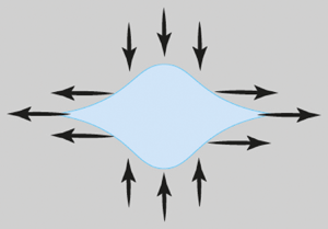
  $1/9$ (obtained by self-similarity analysis) at the two limits of a very thick and a very thin pre-wetting layer, respectively. In the insets, we show a simplified sketch of our system that should illustrate the meaning of our results, and a normalized velocity of the contact line $V/\max \{V\}$ versus the normalized thickness of the pre-wetting layer $H_0/\max \{H_0\}$, for various values of time instances $T\in [9.6\times 10^{-6},1.596\times 10^{-4}]$, where the uppermost curve corresponds to $T=9.6\times 10^{-6}$, the lowermost curve corresponds to $T=1.596\times 10^{-4}$, and the time difference between any two adjacent curves (the time corresponding to any curve minus the time corresponding to the curve just above it) is $10^{-6}$.
5. Conclusions
In this work, we studied the effect of the pre-wetting layer thickness on the propagation rate of the peeling front of fluid that is situated between two infinitely deep and long elastic solids or between an elastic solid and a rigid substrate. We solved the dynamic problem numerically in two limits, a relatively thin and a relatively thick pre-wetting layer. Moreover, we found the corresponding self-similar solution in each of these two limits, and obtained excellent agreement between the dynamic and self-similar solutions in both cases.
Our findings show that in the linear limit, the peeling front propagates at rate  $t^{1/3}$, while in the nonlinear case, it propagates at rate $t^{1/9}$. When compared to the results of Lister et al. (Reference Lister, Peng and Neufeld2013), who found that the peeling front propagates at rates $t^{7/22}$ and $t^{3/8}$ (for pulling and bending limits, respectively), it is clear that the front propagation is slower for the limit of very thick elastic layers. In order to obtain a dependence of the peeling front propagation rate on the pre-wetting layer thickness, we simulated our dynamic nonlinear solver for a range of pre-wetting layer thicknesses, between the limits of a relatively thin and a relatively thick pre-wetting layer. We found that the peeling front propagation scales as time to the powers that constitute a monotone increasing function of the pre-wetting layer thickness, and accept the values within the range $[1/9,1/3]$, where $\lim _{H_0\to 0}\alpha (H_0)\approx 1/9$ and $\lim _{H_0\to H(0,0)}\alpha (H_0)\approx 1/3$, exactly as expected by the self-similarity analysis.
Declaration of interests
The authors report no conflict of interest.
Appendix A. Numerical procedure
A.1. Case 1: linear dynamic problem (under the assumption that $h_0\gg d^*$)

In this case, we solve the non-dimensional linear problem
 \begin{gather} \frac{\partial D}{\partial T}=\frac{1}{12R}\,\frac{\partial}{\partial R}\left(R\,\frac{\partial P}{\partial R}\right), \quad R\in(0,1),\end{gather}
 \begin{gather} D(R,T)=\frac{8}{\rm \pi}\int_0^1 \frac{\partial P}{\partial Y}\,\mathcal{K}(Y,R)\,{\rm d}Y+\frac{8\sqrt{1-R^2}}{\rm \pi}\int_0^1\frac{Y\,P(Y,T)}{\sqrt{1-Y^2}}\,{\rm d}Y, \end{gather}
subject to the boundary and initial conditions
 \begin{gather} \left.\frac{\partial P}{\partial R}\right|_{R=0}=0, \quad T\in(0,T_{fin}),\end{gather}
 \begin{gather} P(R=1,T)=0, \quad T\in(0,T_{fin}), \end{gather}
 \begin{gather} D(R,T=0)=\begin{cases} H_{max}(1-q^2 R^2), & \text{for $R\in[0,1/q],$}\\ 0, & \text{for $R\in(1/q,1],$} \end{cases} \end{gather}
where  $H_{max}$ and $q\gg 1$ are some constants, and where the kernel $\mathcal {K}(Y,R)$ in (A1b) is given in (2.9).
From (A1a), we get that
 \begin{equation} \frac{\partial D}{\partial T}=\frac{1}{12}\frac{\partial^2 P}{\partial R^2}+\frac{1}{12R}\frac{\partial P}{\partial R}, \quad R\in(0,1). \end{equation}
 We solve the coupled system in (A1a,b) by using implicit finite difference scheme. More specifically, we define an equispaced grid in  $R$ that is staggered near $R=0$ and regular near $R=1$, with increment size $\Delta R$ and number of nodes $I$ (the node $1$ is located at $R=\Delta R/2$, and the node $I+1$ is located on the boundary $R=1$), and step forward in time with time step size $\Delta T$. For brevity, we use the notation
 \begin{equation} D_i^n:=D({i}\,{\rm \Delta} R, n\,\Delta T). \end{equation}
Thus at each time level, we solve a linear system with  $2I$ unknowns:
 \begin{equation} u=(D^{n+1}_1,D^{n+1}_2,\ldots,D_I^{n+1},P^{n+1}_1,P^{n+1}_2,\ldots,P^{n+1}_I). \end{equation}
 More specifically, discretising (A3), we get that for  $i=2,\ldots,I-1$, the scheme is given by
 \begin{align} & D_i^{n+1}-\frac{\Delta T}{12\,\Delta
R^2}\,(P^{n+1}_{i+1}-2P^{n+1}_i+P^{n+1}_{i-1})-\frac{\Delta T}{24R_i\,\Delta
R}\,(P^{n+1}_{i+1}-P^{n+1}_{i-1})=D_i^n, \notag\\ & \quad n=0,1,\ldots,N,
\end{align}
\begin{align} & D_i^{n+1}-\frac{\Delta T}{12\,\Delta
R^2}\,(P^{n+1}_{i+1}-2P^{n+1}_i+P^{n+1}_{i-1})-\frac{\Delta T}{24R_i\,\Delta
R}\,(P^{n+1}_{i+1}-P^{n+1}_{i-1})=D_i^n, \notag\\ & \quad n=0,1,\ldots,N,
\end{align}
where  $D^0_i$, $i=1,\ldots,I$, is determined according to the initial conditions in (A2c). These equations yield entries in rows $i=2,\ldots,I-1$ in the mass matrix and the forcing vector as follows:
 \begin{equation} \left.\begin{gathered} M_{i,i}=1,\\ M_{i,i+I}=\dfrac{\Delta T}{6\,\Delta R^2},\\[10pt] M_{i,i+I+1}=-\dfrac{\Delta T}{12\,\Delta R^2}-\dfrac{\Delta T}{24R_i\,\Delta R},\\[10pt] M_{i,i+I-1}=-\dfrac{\Delta T}{12\,\Delta R^2}+\dfrac{\Delta T}{24R_i\,\Delta R} \end{gathered} \right\}\end{equation}
and
 \begin{equation} F_i=D_i^n \quad \text{for all $i=1,2,\ldots,I$}. \end{equation}
For  $i=1$, we use the no-flux boundary condition $(\partial P/\partial R)|_{R=0}=0$, and because we employ a staggered grid, we readily get that
 \begin{equation} D_1^{n+1}-\frac{\Delta T}{12\,\Delta R^2}\,(P^{n+1}_{2}-P^{n+1}_1)-\frac{\Delta T}{24R_1\,\Delta R}\,(P^{n+1}_{2}-P^{n+1}_{1})=D_1^n, \quad n=0,1,\ldots,N, \end{equation}
so that
 \begin{equation} \left.\begin{gathered} M_{1,1}=1,\\ M_{1,I+1}=\dfrac{\Delta T}{12\,\Delta R^2}+\dfrac{\Delta T}{24R_1\,\Delta R},\\[10pt] M_{1,I+2}=-\dfrac{\Delta T}{12\,\Delta R^2}-\dfrac{\Delta T}{24R_1\,\Delta R}. \end{gathered} \right\}\end{equation}
For  $i=I$, we use the boundary condition near $R=1$, namely that $P_{I+1}=0$, so that we get
 \begin{equation} D_I^{n+1}-\frac{\Delta T}{12\,\Delta R^2}\,(-2P^{n+1}_I+P^{n+1}_{I-1})+\frac{\Delta T\, P^{n+1}_{I-1}}{24R_I\,\Delta R}=D_I^n, \quad n=0,1,\ldots,N, \end{equation}
which yields
 \begin{equation} \left.\begin{gathered} M_{I,I}=1,\\ M_{I,2I}=\dfrac{\Delta T}{6\,\Delta R^2},\\[10pt] M_{I,2I-1}=-\dfrac{\Delta T}{12\,\Delta R^2}+\dfrac{\Delta T}{24R_i\,\Delta R}. \end{gathered} \right\}\end{equation}
To discretise the equation in (A1b), we use the trapezoidal rule, which results in
 \begin{align} &D_i^{n+1}-\frac{4\,{\rm \Delta} R}{\rm \pi}\left[\left.\mathcal{K}_{1,i}\left(\frac{\partial P}{\partial Y}\right)\right|_{Y=Y_1}+2\mathcal{K}_{2,i}\left.\left(\frac{\partial P}{\partial Y}\right)\right|_{Y=Y_2}+\cdots+2\mathcal{K}_{I-1,i}\left.\left(\frac{\partial P}{\partial Y}\right)\right|_{Y=Y_{I-1}}\right.\nonumber\\ &\quad \left.\left. {}+2\mathcal{K}_{I,i}\left(\frac{\partial P}{\partial Y}\right)\right|_{Y=Y_I} +\mathcal{K}_{I+1,i}\left.\left(\frac{\partial P}{\partial Y}\right)\right|_{Y=Y_{I+1}}+ \frac{1}{2}\,\mathcal{K}_{1,i}\left.\left(\frac{\partial P}{\partial Y}\right)\right|_{Y=Y_1}\right]\nonumber\\ &\quad -\frac{4\,\Delta R\,\sqrt{1-R_i^2}}{\rm \pi}\left(\frac{R_1P_1^{n+1}}{\sqrt{1-R_1^2}}+\frac{2R_2P_2^{n+1}}{\sqrt{1-R_2^2}} +\cdots+\frac{2R_{I-1}P_{I-1}^{n+1}}{\sqrt{1-R_{I-1}^2}}+\frac{R_IP_I^{n+1}}{\sqrt{1-R_I^2}}\right.\nonumber\\ &\quad \left.{}+\frac{R_1P_1^{n+1}}{2\sqrt{1-R_1^2}}+\frac{R_I P_I^{n+1}}{2\sqrt{1-R_I^2}}\right)=0. \end{align}
Note that the term
 \begin{equation} \frac{1}{2}\,\mathcal{K}_{1,i}\left.\left(\frac{\partial P}{\partial Y}\right)\right|_{Y=Y_1} \end{equation}
that appears on the second line of (A13) accounts for the contribution to the integral from the interval  $[0,Y_1]$, whose length is $\Delta R/2$, and where we use the boundary conditions according to which $(\partial P/\partial R)|_{R=0}=0$, and assume that (approximately) the derivative $\partial P/\partial R$ is a linear function on $[0,Y_1]$ (similar assumption to the trapezoidal rule). For the same reason, the terms
 \begin{equation} \frac{R_1P_1^{n+1}}{2\sqrt{1-R_1^2}} \quad \text{and} \quad \frac{R_IP_I^{n+1}}{2\sqrt{1-R_I^2}} \end{equation}
appear on the fourth line of (A13), where implicit here is the assumption that the function  $R\,P(R)/\sqrt {1-R^2}$ is sufficiently regular near $R=0$ and $R=1$, and tends to $0$ as $R\to 0$ and $R\to 1$ (because of the boundary condition near $R=1$, by which $P(R=1,T)=0$).
To simplify the expression in (A13), we use central differences for the first-order derivative of  $P$ at interior nodes, no-flux boundary conditions near $R=0$, which imply that
 \begin{equation} \left.\left(\frac{\partial P}{\partial Y}\right)\right|_{Y=Y_1}=\frac{1}{2\,\Delta Y}\,(P_2-P_1)+O(\Delta Y^2), \end{equation}
and backward difference near the boundary  $R=1$, subject to the boundary condition that $P(R=1,T)=0$, namely
 \begin{align} \left.\left(\frac{\partial P}{\partial Y}\right)\right|_{Y=Y_{I+1}}&=\frac{1}{\Delta Y}\left(\frac{3}{2}\,P_{I+1}-2P_I+\frac{1}{2}\,P_{I-1}\right)+O(\Delta Y^2)\nonumber\\ &=\frac{1}{\Delta Y}\left(-2P_I+\frac{1}{2}\,P_{I-1}\right)+O(\Delta Y^2). \end{align}
Thus we get from (A13) that
 \begin{align} &D_i^{n+1}-\frac{2}{\rm \pi}\left[\frac{3}{2}\,\mathcal{K}_{1,i}(P^{n+1}_2-P^{n+1}_1)+2 \mathcal{K}_{2,i}(P^{n+1}_3-P^{n+1}_1)+\cdots+2\mathcal{K}_{I-1,i}(P^{n+1}_I-P^{n+1}_{I-2})\right.\nonumber\\ &\quad \left. {}-2\mathcal{K}_{I,i}P^{n+1}_{I-1} +2\mathcal{K}_{I+1,i}\left(-2P^{n+1}_I+\frac{1}{2}\,P^{n+1}_{I-1}\right)\right]\nonumber\\ &\quad -\frac{4\,\Delta R\,\sqrt{1-R_i^2}}{\rm \pi}\left(\frac{3R_1P_1^{n+1}}{2\sqrt{1-R_1^2}}+\frac{2R_2P_2^{n+1}}{\sqrt{1-R_2^2}} +\cdots+\frac{2R_{I-1}P_{I-1}^{n+1}}{\sqrt{1-R_{I-1}^2}}\right.\nonumber\\ &\quad \left.+\frac{3R_I P_I^{n+1}}{2\sqrt{1-R_I^2}}\right)=0, \quad i=1,\ldots,I. \end{align}
This results in an additional  $I$ equations (for the $P_i$), i.e. for $i=1,\ldots,I$, we may fill the rows $I+i$ of the mass matrix as follows:
 \begin{equation} \left.\begin{gathered} M_{I+i,i}=1,\\ M_{I+i,I+1}=\dfrac{1}{\rm \pi}\left(3\mathcal{K}_{1,i}+4\mathcal{K}_{2,i}-\dfrac{6R_1\,\Delta R\,\sqrt{1-R_i^2}}{\sqrt{1-R_1^2}}\right),\\[18pt] M_{I+i,I+2}=\dfrac{1}{\rm \pi}\left(-3\mathcal{K}_{1,i}+4\mathcal{K}_{3,i}-\dfrac{8R_2\,\Delta R\,\sqrt{1-R_i^2}}{\sqrt{1-R_2^2}}\right),\\[18pt] M_{I+i,I+s}=\dfrac{1}{\rm \pi}\left(-4\mathcal{K}_{s-1,i}+4\mathcal{K}_{s+1,i}-\dfrac{8R_s\,\Delta R\,\sqrt{1-R_i^2}}{\sqrt{1-R_s^2}}\right), \quad s=3,4,\ldots,I-2,\\[18pt] M_{I+i,2I-1}=\dfrac{1}{\rm \pi}\left(-4\mathcal{K}_{I-2,i}+4\mathcal{K}_{I,i}-2\mathcal{K}_{I+1,i}-\dfrac{8R_{I-1}\,\Delta R\,\sqrt{1-R_i^2}}{\sqrt{1-R_{I-1}^2}}\right),\\[18pt] M_{I+i,2I}=\dfrac{1}{\rm \pi}\left(-4\mathcal{K}_{I-1,i}+8\mathcal{K}_{I+1,i}-\dfrac{6R_I\,\Delta R\,\sqrt{1-R_i^2}}{\sqrt{1-R_I^2}}\right), \end{gathered} \right\}\end{equation}
and the forcing vector vanishes,  $F_{I+i}=0$, for all $i=1,2,\ldots,I$.
Then using (A7), (A8), (A10), (A12) and (A19), we solve the linear system
 \begin{equation} Mu^{n+1}=F, \end{equation}
update  $D$ by setting $D_i^{n+1}=u_{i}^{n+1}$, $i=1,\ldots,I$, and move to the next time level.
A.2. Case 2: linear self-similar problem (under the assumption that $h_0\gg d^*$)

In this case, we solve the problem
 \begin{equation} \left.\begin{gathered} 8\tilde{D}+4\eta\,\frac{{\rm d}\tilde{D}}{{\rm d}\eta}+\frac{1}{\eta}\,\frac{{\rm d}}{{\rm d}\eta} \left(\eta\,\frac{{\rm d}\tilde{P}}{{\rm d}\eta}\right)=0,\\ \tilde{D}(\eta)=L^3\left[\frac{8}{\rm \pi}\int_0^1 \frac{\partial \tilde{P}}{\partial \xi}\, \mathcal{K}(\xi,\eta)\,{\rm d}\xi+\frac{8\sqrt{1-\eta^2}}{\rm \pi}\int_0^1\frac{\xi\, \tilde{P}(\xi)}{\sqrt{1-\xi^2}}\,{\rm d}\xi\right], \end{gathered}\right\} \end{equation}
subject to the following boundary conditions and constraints:
 $$\begin{gather} \left.\frac{{\rm d}\tilde{D}}{{\rm d}\eta}\right|_{\eta=0}=0, \end{gather}$$
 $$\begin{gather}\left.\frac{{\rm d}\tilde{D}}{{\rm d}\eta}\right|_{\eta=1}=0, \end{gather}$$
 $$\begin{gather}L=\begin{pmatrix}\displaystyle\frac{\Delta V}{\displaystyle 2{\rm \pi}\int_{0}^1 \tilde{D}\eta \,{\rm d}\eta}\end{pmatrix}^{1/3}. \end{gather}$$
In practice, we find the solution to (A21) subject to (A22)–(A24) iteratively. First, we replace the constraint in (A23) by
 \begin{equation} \tilde{D}(\eta=0)=\tilde{D}_0, \end{equation}
where  $\tilde {D}_0$ will be determined by using a bisection method during the solution process, as we will explain in the sequel, so that the condition in (A23) will be satisfied.
We have iterations of two types. In the first type, we start with some initial guess for  $\tilde {D}_0$, such that $\tilde {D}_0>0$, and perform the iterative procedure, which converges to the solution of (A21), so that the boundary conditions in (A22)–(A24) are satisfied. In the iterations of the second type, for each given $\tilde {D}_0$, such that $\tilde {D}_0>0$, we solve (A21), subject to (A22) and an artificial boundary condition
 \begin{equation} \tilde{P}(\eta=1)=C, \end{equation}
rather than (A24), where  $C$ is some initial guess for which the solution exists, $C\neq 0$. Note that according to our verification, the specific choice of $C$ does not affect the solution, and the only reason for prescribing it is to prevent the solver from convergence to a trivial solution (namely, $\tilde {D}=0$). These iterations of the second type proceed as follows. We denote the solution of the system in (A21) subject to (A22) and (A26) (and with some initial guess for $L$ denoted by $L^{(0)}$) by $\tilde {D}_{temp}(\eta )$. Next, we move to the next iteration by updating the solution, which we denote by $\tilde {D}^{(1)}(\eta )$, by using
 \begin{equation} \tilde{D}^{(1)}(\eta)=\frac{\tilde{D}_0}{\tilde{D}_{temp}(0)}\,\tilde{D}_{temp}(\eta). \end{equation}
Note that since the problem in (A21) is linear and  $\tilde {D}_{temp}(\eta )$ satisfies it, also $\tilde {D}^{(1)}(\eta )$ satisfies (A21), because $\tilde {D}_{temp}(\eta )$ and $\tilde {D}^{(1)}(\eta )$ differ only by multiplication by a constant. Moreover, since $\tilde {D}_{temp}(\eta )$ satisfies the boundary condition in (A22), so does $\tilde {D}^{(1)}(\eta )$. Furthermore, $\tilde {D}^{(1)}(\eta )$ satisfies the condition in (A25) (which follows by the construction). However, in order to satisfy the volume constraint in (A24), we update $L$ at the current iteration by using (A24) with $\tilde {D}^{(1)}(\eta )$ substituted instead of $\tilde {D}(\eta )$, and denote the result by $L^{(1)}$. Now, having found $L^{(1)}$, we repeat the same procedure: calculate a new $\tilde {D}_{temp}(\eta )$, then by using (A27), we find $\tilde {D}^{(2)}(\eta )$, and then calculate $L^{(2)}$, and so on, until convergence is achieved (that is, the difference between $L$ obtained at adjacent iterations satisfies $|L^{(k)}-L^{(k-1)}|<\delta$, where $0<\delta \ll 1$ denotes some prescribed tolerance.)
Note that the limiting solution, which we denote by  $\tilde {D}(\eta ;\tilde {D}_0)$ (which was obtained in the iterations of the second type), satisfies the problem in (A21), the boundary conditions (A22) and (A25), and the volume constraint in (A24), so that the only condition that is still needed to be satisfied is (A23). Since we have one degree of freedom, which is $\tilde {D}_0$ in the condition in (A25), we may modify $\tilde {D}_0$ so that the condition in (A23) will be satisfied (and this constitutes the first type of iterations). This is because according to our verification, for a sufficiently large $\tilde {D}_0$ we have $\textrm {d}\tilde {D}(\eta ;\tilde {D}_0)/\textrm {d}\eta >0$, for a sufficiently small $\tilde {D}_0$ we have $\textrm {d}\tilde {D}(\eta ;\tilde {D}_0)/\textrm {d}\eta <0$, and $\textrm {d}\tilde {D}(\eta ;\tilde {D}_0)/\textrm {d}\eta$ is a continuous and monotone increasing function of $\tilde {D}_0$. Thus there exists $\tilde {D}_0$ such that $\textrm {d}\tilde {D}(\eta ;\tilde {D}_0)/\textrm {d}\eta =0$. Numerically, it is possible to find $\tilde {D}_0$ by e.g. the bisection method, where we request that $|\textrm {d}\tilde {D}(\eta ;\tilde {D}_0)/\textrm {d}\eta |<\delta _1$, where $0<\delta _1\ll 1$ is some prescribed tolerance.
In our results presented in figure 2, the tolerances that we have set were  $\delta =10^{-5}$ and $\delta _1=10^{-6}$.
Now we will explain in detail our methodology for the solution of the system in (A21) subject to (A22) and (A26). Specifically, we solve the system in (A21) in a manner similar to the method discussed in the previous section. That is, by using finite differences, we discretise the ODE in (A21) for  $i=2,\ldots,I-1$ as
 \begin{align} 8\tilde{D}_i+\frac{2\eta_i}{\Delta \eta} \left(\tilde{D}_{i+1}-\tilde{D}_{i-1}\right)+\frac{1}{\Delta \eta^2}\left(\tilde{P}_{i+1}-2\tilde{P}_i+\tilde{P}_{i-1}\right)+\frac{1}{2\eta_i\, \Delta\eta} \left(\tilde{P}_{i+1}-\tilde{P}_{i-1}\right)=0. \end{align}
This results in the following rows of the mass matrix:
 \begin{equation} \left.\begin{gathered} M_{i,i}=8,\\ M_{i,i+1}=\dfrac{2\eta_i}{\Delta \eta},\\ M_{i,i-1}=-\dfrac{2\eta_i}{\Delta \eta},\\ M_{i,I+i}=-\dfrac{2}{\Delta \eta^2},\\ M_{i,I+i+1}=\dfrac{1}{\Delta \eta^2}+\dfrac{1}{2\eta_i\,\Delta\eta},\\ M_{i,I+i-1}=\dfrac{1}{\Delta \eta^2}-\dfrac{1}{2\eta_i\,\Delta\eta}. \end{gathered} \right\}\end{equation}
Near the boundary  $\eta =0$, we use the boundary condition in (A22) for $\tilde {D}$ and a one-sided derivative for $\tilde {P}$. Thus for $i=1$, we get that
 \begin{align} &8\tilde{D}_1+\frac{2\eta_1}{\Delta \eta} \left(\tilde{D}_{2}-\tilde{D}_{1}\right)+ \frac{1}{\Delta \eta^2}\left(2\tilde{P}_{1}-5\tilde{P}_2+4\tilde{P}_{3}-\tilde{P}_4\right)\nonumber\\ &\quad+\frac{1}{\eta_1\,\Delta\eta} \left(-1.5\tilde{P}_{1}+2\tilde{P}_{2}-0.5\tilde{P}_3\right)=0. \end{align}
This results in the following entries in the first row of the mass matrix:
 \begin{equation} \left.\begin{gathered} M_{1,1}=8-\dfrac{2\eta_1}{\Delta \eta},\\ M_{1,2}=\dfrac{2\eta_1}{\Delta \eta},\\ M_{1,I+1}=\dfrac{2}{\Delta \eta^2}-\dfrac{3}{2\eta_1\,\Delta\eta},\\ M_{1,I+2}=-\dfrac{5}{\Delta \eta^2}+\dfrac{2}{\eta_1\,\Delta\eta},\\ M_{1,I+3}=\dfrac{4}{\Delta \eta^2}-\dfrac{1}{2\eta_1\,\Delta\eta},\\ M_{1,I+4}=-\dfrac{1}{\Delta \eta^2}. \end{gathered} \right\}\end{equation}
As to the forcing vector, we get that
 \begin{equation} F_i=0, \quad i=1,\ldots,I-1. \end{equation}
 Near the boundary  $\eta =1$, we use a one-sided derivative for $\tilde {D}$ and the boundary condition in (A26) for $\tilde {P}$. Thus for $i=I$, we get that
 \begin{align} &8\tilde{D}_I+\frac{4\eta_I}{\Delta \eta} \left(1.5\tilde{D}_{I}-2\tilde{D}_{I-1}+0.5\tilde{D}_{I-2}\right)+ \frac{1}{\Delta \eta^2}\left(C-2\tilde{P}_I+\tilde{P}_{I-1}\right)\nonumber\\ &\quad + \frac{1}{2\eta_I\,\Delta\eta} \left(C-\tilde{P}_{I-1}\right)=0. \end{align}
This results in the following entries in the Ith row of the mass matrix:
 \begin{equation} \left.\begin{gathered} M_{I,I}=8+\dfrac{6\eta_I}{\Delta \eta},\\ M_{I,I-1}=-\dfrac{8\eta_I}{\Delta \eta},\\ M_{I,I-2}=\dfrac{2\eta_I}{\Delta \eta},\\ M_{I,2I}=-\dfrac{2}{\Delta \eta^2},\\ M_{I,2I-1}=\dfrac{1}{\Delta \eta^2}-\dfrac{1}{2\eta_I\,\Delta\eta}. \end{gathered} \right\}\end{equation}
The forcing vector term is
 \begin{equation} F_I=-\frac{C}{\Delta \eta^2}-\frac{C}{2\eta_I\,\Delta \eta}. \end{equation}
A.3. Case 3: nonlinear dynamic problem (under the assumption that $h_0\ll d^*$)

In this case, we solve the problem
 $$\begin{gather} \frac{\partial H}{\partial T}=\frac{1}{12 R}\,\frac{\partial}{\partial R}\left( RH^3\,\frac{\partial P}{\partial R}\right), \quad R\in(0,1), \end{gather}$$
 $$\begin{gather}D(R,T)=\frac{8}{\rm \pi}\int_0^1 \frac{\partial P}{\partial Y}\,\mathcal{K}(Y,R)\,{\rm d}Y+\frac{8\sqrt{1-R^2}}{\rm \pi}\int_0^1\frac{Y\,P(Y,T)}{\sqrt{1-Y^2}}\,{\rm d}Y, \end{gather}$$
subject to the boundary and initial conditions
 \begin{equation} \left.\begin{gathered}
\left.\frac{\partial P}{\partial R}\right|_{R=0}=0, \quad
T\in(0,T_{fin}),\\ \left.\frac{\partial P}{\partial
R}\right|_{R=1}=0, \quad T\in(0,T_{fin}),\\
D(R,T=0)=\begin{cases} (H_{max}-H_0)(1-q^2 R^2), & \text{for
$R\in[0,1/q],$}\\ 0, & \text{for $R\in(1/q,1],$}
\end{cases} \end{gathered}\right\}
\end{equation}
\begin{equation} \left.\begin{gathered}
\left.\frac{\partial P}{\partial R}\right|_{R=0}=0, \quad
T\in(0,T_{fin}),\\ \left.\frac{\partial P}{\partial
R}\right|_{R=1}=0, \quad T\in(0,T_{fin}),\\
D(R,T=0)=\begin{cases} (H_{max}-H_0)(1-q^2 R^2), & \text{for
$R\in[0,1/q],$}\\ 0, & \text{for $R\in(1/q,1],$}
\end{cases} \end{gathered}\right\}
\end{equation}
where  $H_{max}$ and $q\gg 1$ are some prescribed constants.
In order to allow simulations with small values of  $H_0$, namely $0< H_0\ll H_{max},$ one needs to use a very dense grid in the vicinity of the front. However, in the rest of the domain, such a dense grid is not needed. In this subsection, let us explain our methodology for solving the above problem over an adjustable grid, which is dense near $R=0$ (including the front), and which becomes less dense as we move towards $R=1$.
To set an adjustable grid, let us define the transformation
 \begin{equation} R=\left(X-\frac{1}{q}\right)^{2b+1}-a, \quad 0< a\ll 1, b\in\boldsymbol{N}, \end{equation}
where we will prescribe an equispaced grid on  $X$. A convenient choice for $a$ is $a=1/q$. From (A38), we get that
 \begin{equation} X=\frac{1}{q}+(R+a)^{{1}/({2b+1})}, \end{equation}
and in order to obtain  $R\in (0,1)$, the boundaries of $X$ should be
 \begin{equation} \frac{1}{q}+a^{{1}/({2b+1})}\leqslant X\leqslant \frac{1}{q}+(1+a)^{{1}/({2b+1})}. \end{equation}
It is easy to verify that when we set an equispaced grid in the  $X$-coordinate, this results in a non-uniform grid in $R$ that is the most dense near $R=0$ and becomes less dense towards $R=1$, as desired.
In order to solve our problem on a uniform grid, we need to transform our problem to the  $X$-coordinate, and then solve it on an equispaced grid in $X$. For this, we will use the derivatives
 \begin{equation} \left.\begin{gathered} \frac{{\rm d}X}{{\rm d}R}=\frac{1}{2b+1}\,(R+a)^{{1}/({2b+1})-1},\\ \frac{{\rm d}^2 X}{{\rm d}R^2}=\frac{1}{2b+1}\left(\frac{1}{2b+1}-1\right)(R+a)^{{1}/({2b+1})-2}. \end{gathered}\right\} \end{equation}
Note that since  $a>0$, these derivatives are not singular in the range $R\in (0,1)$. Substituting this into the PDE in (A36), we get that for $X\in ({1}/{q}+a^{{1}/({2b+1})},{1}/{q}+ (1+a)^{{1}/({2b+1})})$,
 \begin{equation} \frac{\partial
H}{\partial T}=H^3\,\frac{\partial^2 P}{\partial
X^2}\left(\frac{{\rm d}X}{{\rm
d}R}\right)^2+H^3\,\frac{\partial P}{\partial
X}\,\frac{{\rm d}^2 X}{{\rm d}R^2}+3H^2\,\frac{\partial
H}{\partial X}\,\frac{\partial P}{\partial
X}\left(\frac{{\rm d}X}{{\rm
d}R}\right)^2+\frac{H^3}{R}\,\frac{\partial P}{\partial
X}\,\frac{{\rm d}X}{{\rm d}R}.
\end{equation}
\begin{equation} \frac{\partial
H}{\partial T}=H^3\,\frac{\partial^2 P}{\partial
X^2}\left(\frac{{\rm d}X}{{\rm
d}R}\right)^2+H^3\,\frac{\partial P}{\partial
X}\,\frac{{\rm d}^2 X}{{\rm d}R^2}+3H^2\,\frac{\partial
H}{\partial X}\,\frac{\partial P}{\partial
X}\left(\frac{{\rm d}X}{{\rm
d}R}\right)^2+\frac{H^3}{R}\,\frac{\partial P}{\partial
X}\,\frac{{\rm d}X}{{\rm d}R}.
\end{equation}
In other words, this equation may be expressed for  $X\in(\frac{1}{q}+a^{{1}/({2b+1})},\frac{1}{q}+ (1+a)^{{1}/({2b+1})})$ as,
 \begin{gather}
\frac{\partial H}{\partial T}=A H^3\,\frac{\partial^2
P}{\partial X^2}+B H^3\,\frac{\partial P}{\partial X}+3A
H^2\,\frac{ \partial H}{\partial X}\,\frac{\partial
P}{\partial
X}+C\,\frac{H^3}{R}\,\frac{\partial
P}{\partial X},
\end{gather}
\begin{gather}
\frac{\partial H}{\partial T}=A H^3\,\frac{\partial^2
P}{\partial X^2}+B H^3\,\frac{\partial P}{\partial X}+3A
H^2\,\frac{ \partial H}{\partial X}\,\frac{\partial
P}{\partial
X}+C\,\frac{H^3}{R}\,\frac{\partial
P}{\partial X},
\end{gather}where
 \begin{equation} \left.\begin{gathered} A:=\left(\frac{{\rm d}X}{{\rm d}R}\right)^2=\left[\frac{1}{2b+1}\,(R+a)^{{1}/({2b+1})-1}\right]^2,\\ B:=\frac{{\rm d}^2 X}{{\rm d}R^2}=\frac{1}{2b+1}\left(\frac{1}{2b+1}-1\right)(R+a)^{{1}/({2b+1})-2},\\ C:=\frac{{\rm d}X}{{\rm d}R}=\frac{1}{2b+1}\,(R+a)^{{1}/({2b+1})-1}. \end{gathered}\right\} \end{equation}
Following, a known methodology (see e.g. Ozawa, Nishitani & Doi Reference Ozawa, Nishitani and Doi2005; Zigelman & Novick-Cohen Reference Zigelman and Novick-Cohen2021), we linearise the equation given in (A43) about the solution at some given current time level, taking in each nonlinear term the highest-order derivative on the next time level, and the remaining terms, which involve derivatives of the same or lower orders, on the current time level; here, we regard  $P$ as a function with higher priority than $H$ to be evaluated on the next time level, because $P$ is expected to have higher singularity near the peeling front. More specifically, we evaluate all of the lower-order derivatives at the previous time level, and the higher-order derivatives at the current time level. Thus we get
 \begin{align} &H^{n+1}-A\,\Delta T\,(H^{n})^3\,\frac{\partial^2 P^{n+1}}{\partial X^2}-B\,\Delta T\,(H^{n})^3\,\frac{\partial P^{n+1}}{\partial X}\nonumber\\ &\quad -3A\,\Delta T\,(H^{n})^2\,\frac{\partial H^{n}}{\partial X}\,\frac{\partial P^{n+1}}{\partial X}-C\,\Delta T\,\frac{(H^{n})^3}{R}\,\frac{\partial P^{n+1}}{\partial X}=H^{n}, \quad n=0,1,\ldots,N. \end{align}
To obtain the mass matrix, it remains to discretise the equation in (A45) in space, for which we use central differences, as discussed previously.
As to the boundary conditions in terms of  $X$, we get, for example, that
 \begin{equation} \left.\frac{\partial P}{\partial X}\right|_{X={1}/{q}+a^{{1}/({2b+1})}}=\left.\frac{\partial P}{\partial R}\right|_{R=0}\left.\frac{{\rm d}R}{{\rm d}X}\right|_{X={1}/{q}+a^{{1}/({2b+1})}}=0, \end{equation}
and similarly for all other boundary conditions.
It remains to discuss how this change of variables affects the integral equation. However, before transforming the coordinates, let us rewrite the second integral in (A36b) in a more convenient manner, applying integration by parts, as
 \begin{align} \int_0^1 \frac{Y\,P(Y,T)}{\sqrt{1-Y^2}}\,{\rm d}Y&=-\sqrt{1-Y^2}\,P|_{0}^1+\int_0^1\frac{\partial P}{\partial Y}\,\sqrt{1-Y^2}\,{\rm d}Y\nonumber\\ &=P(0,T)+\int_0^1\frac{\partial P}{\partial Y}\,\sqrt{1-Y^2}\,{\rm d}Y. \end{align}
Now let us substitute (A47) into (A36b) and transform the variable  $Y$ to $Z$, where $Z$ is defined in a similar manner to $X$, namely
 \begin{equation} Z=\frac{1}{q}+(R+a)^{{1}/({2b+1})}. \end{equation}
Thus we may regard the kernel  $\mathcal {K}$ as a function of $X,Z$. In other words, we may define $\tilde {\mathcal {K}}(Z,X):=\mathcal {K}(Y(Z),R(X))$. Hence changing variables from $R,Y$ to $X,Z$ in (A36b), we get that
 \begin{align} D(X,T)&=\frac{8}{\rm \pi}\int_{{1}/{q}+a^{{1}/{2b}}}^{{1}/{q}+(1+a)^{{1}/{2b}}} \frac{\partial P}{\partial Z}\,\tilde{\mathcal{K}}(Z,X)\,{\rm d}Z \nonumber\\ &\quad +\frac{8}{\rm \pi}\,\sqrt{1-R(X)^2}\left[P(0,T)+\int_0^1\frac{\partial P}{\partial Z}\,\sqrt{1-Y(Z)^2}\,{\rm d}Z\right]. \end{align}
 Next, using an equispaced grid for  $X$, so that our nodal points are $X_i$, $i=1,\ldots,I$, employing the ‘no-flux’ boundary conditions at $R=0,1$, and discretising the equation in (A49), we get that
 \begin{align} &D_i^{n+1}-\frac{2}{\rm \pi}\left[\frac{3}{2}\,\tilde{\mathcal{K}}_{1,i}(P^{n+1}_2-P^{n+1}_1)+2\tilde{\mathcal{K}}_{2,i}(P^{n+1}_3-P^{n+1}_1)+\cdots+2\tilde{\mathcal{K}}_{I-1,i}(P^{n+1}_I-P^{n+1}_{I-2}) \right.\nonumber\\ &\quad \left.{}+\frac{3}{2}\,\tilde{\mathcal{K}}_{I,i}(P^{n+1}_I-P^{n+1}_{I-1})\right]\nonumber\\ &\quad -\frac{2\sqrt{1-R_i^2}}{\rm \pi}\left[4P^{n+1}_1+\frac{3}{2}\,(P^{n+1}_2-P^{n+1}_1)\sqrt{1-R_1^2}+2(P^{n+1}_3-P^{n+1}_1)\sqrt{1-R_2^2} \right.\nonumber\\ &\quad \left. +\cdots+2(P^{n+1}_I-P^{n+1}_{I-2})\sqrt{1-R_{I-1}^2}+\frac{3}{2}\,(P^{n+1}_I-P^{n+1}_{I-1})\sqrt{1-R_I^2}\right]=0, \quad i=1,\ldots,I. \end{align}
This results in the following rows of the mass matrix:
 \begin{equation} \left.\begin{gathered} M_{I+i,i}=1,\\ M_{I+i,I+1}=\dfrac{1}{\rm \pi}\left(3\tilde{\mathcal{K}}_{1,i}+4\tilde{\mathcal{K}}_{2,i}-8\sqrt{1-R_i^2}+3\sqrt{(1-R_i^2)(1-R_1^2)}+4\sqrt{(1-R_i^2)(1-R_2^2)}\right),\\ M_{I+i,I+2}=\dfrac{1}{\rm \pi}\left(-3\tilde{\mathcal{K}}_{1,i}+4\tilde{\mathcal{K}}_{3,i}-3\sqrt{(1-R_i^2)(1-R_1^2)}+4\sqrt{(1-R_i^2)(1-R_3^2)}\right),\\ M_{I+i,I+s}=\dfrac{1}{\rm \pi}\left(-4\tilde{\mathcal{K}}_{s-1,i}+4\tilde{\mathcal{K}}_{s+1,i}-4\sqrt{(1-R_i^2)(1-R_{s-1}^2)}+4\sqrt{(1-R_i^2)(1-R_{s+1}^2)}\right),\\ \quad\quad\quad\quad\quad s=3,4,\ldots,I-2,\\ M_{I+i,2I-1}=\dfrac{1}{\rm \pi}\left(-4\tilde{\mathcal{K}}_{I-2,i}+3\tilde{\mathcal{K}}_{I,i}-4\sqrt{(1-R_i^2)(1-R_{I-2}^2)}+3\sqrt{(1-R_i^2)(1-R_I^2)}\right),\\ M_{I+i,2I}=\dfrac{1}{\rm \pi}\left(-4\tilde{\mathcal{K}}_{I-1,i}-3\tilde{\mathcal{K}}_{I,i}-4\sqrt{(1-R_i^2)(1-R_{I-1}^2)}-3\sqrt{(1-R_i^2)(1-R_I^2)}\right). \end{gathered} \right\}\end{equation}
A.4. Case 4: nonlinear self-similar problem (under the assumption that $h_0\ll d^*$)

In this case, we solve the nonlinear self-similar problem
 $$\begin{gather} 8\tilde{D}+4\eta\,\frac{{\rm d}\tilde{D}}{{\rm d}\eta}+\frac{3}{\eta}\,\frac{{\rm d}}{{\rm d}\eta} \left(\eta\tilde{D}^3\,\frac{{\rm d}\tilde{P}}{{\rm d}\eta}\right)=0, \end{gather}$$
 $$\begin{gather}\tilde{D}(\eta)=\frac{8}{\rm \pi}\int_0^1 \frac{\partial \tilde{P}}{\partial \xi}\,\mathcal{K}(\xi,\eta)\, {\rm d}\xi+\frac{8\sqrt{1-\eta^2}}{\rm \pi}\int_0^1\frac{\xi\,\tilde{P}(\xi)}{\sqrt{1-\xi^2}}\,{\rm d}\xi, \end{gather}$$
subject to the boundary conditions
 $$\begin{gather} \left.\frac{{\rm d}\tilde{D}}{{\rm d}\eta}\right|_{\eta=0}=0, \end{gather}$$
 $$\begin{gather}\tilde{D}(1)=0. \end{gather}$$
To solve this problem numerically, we follow the methodology developed by Peck et al. (Reference Peck, Wrobel, Perkowska and Mishuris2018) and define an auxiliary variable
 \begin{equation} U(\eta)=\eta\tilde{D}^2\,\frac{\partial \tilde{P}}{\partial \eta}, \end{equation}
so that the problem in (A52) may be expressed as
 $$\begin{gather} 8\tilde{D}+4\eta\,\frac{{\rm d}\tilde{D}}{{\rm d}\eta}+\frac{3}{\eta}\,\frac{{\rm d}}{{\rm d}\eta} \left(\tilde{D}U\right)=0, \end{gather}$$
 $$\begin{gather}\tilde{D}(\eta)=\frac{8}{\rm \pi}\int_0^1 \frac{\partial \tilde{P}}{\partial \xi}\,\mathcal{K}(\xi,\eta)\, {\rm d}\xi+\frac{8\sqrt{1-\eta^2}}{\rm \pi}\int_0^1\frac{\xi\,\tilde{P}(\xi)}{\sqrt{1-\xi^2}}\,{\rm d}\xi. \end{gather}$$
Equation (A55a) may be expressed as
 \begin{equation} \frac{{\rm d}}{{\rm d}\eta}(\tilde{D}U)=-\frac{4}{3}\,\frac{{\rm d}}{{\rm d}\eta}(\eta^2\tilde{D}), \end{equation}
which, integrated with respect to  $\hat {\eta }$ in the interval $0\leqslant \hat {\eta }<\eta$, yields that
 \begin{equation} U(\eta)=-\tfrac{4}{3}\eta^2. \end{equation}
 Thus from the definition of  $U$ in (A54), it follows that as far as $\tilde {D}$ is known, $\partial \tilde {P}/\partial \eta$ may be obtained via
 \begin{equation} \frac{\partial \tilde{P}}{\partial \eta}=-\frac{4}{3}\,\frac{\eta}{\tilde{D}^2}, \end{equation}
and  $\tilde {P}$ may be evaluated by integrating (A58) with respect to $\eta$. More specifically, integrating (A58), we get that
 \begin{equation} \tilde{P}(\eta)=-\frac{4}{3}\int_{0}^{\eta}\frac{\hat{\eta}}{\tilde{D}^2}\,{\rm d}\hat{\eta}+\tilde{P}(0), \end{equation}
where  $\tilde {P}(0)$ is a constant of integration, which is determined according to the explanation that follows.
We find  $\tilde {D}$ and $\tilde {P}$ iteratively. Specifically, we start the iterations with some guess for $\tilde {D}$ that has the expected behaviour at $\eta =0,\,1$, e.g. we started our simulations with the initial guess $\tilde {D}^{(0)}={const}./\sqrt {1-\eta ^2}$, where $const.$ is some arbitrary constant, which does not affect the solution. In addition, we set some initial guess for $\tilde {P}(0)$. We solve the problem with these $\tilde {D}^{(0)}(\eta )$ and $\tilde {P}(0)$ values as follows. In the first iteration, we substitute $\tilde {D}^{(0)}(\eta )$ and $\tilde {P}(0)$ into (A59) and thus find $\tilde {P}^{(1)}(\eta )$. Then we substitute $\tilde {P}^{(1)}(\eta )$ into (A55b) and find $\tilde {D}^{(1)}(\eta )$. We continue in the same manner, by alternately substituting $\tilde {D}$ into (A59), substituting the obtained $\tilde {P}$ into (A55b), and so on. We stop this iterative process when the differences in the $L^{\infty }$-norm between the $\tilde {D}$ values and $\tilde {P}$ values in the current and previous iterations are smaller than a prescribed tolerance.
By using this iterative process, we find a solution to (A55) that satisfies the boundary condition in (A53a), but it does not necessarily satisfy the boundary condition in (A53b). Requesting that (A53b) is satisfied implies a constraint on  $\tilde {P}(0)$. This is because, as it is possible to verify, $\tilde {D}(1)$ is a continuous and monotone increasing function of $\tilde {P}(0)$ that satisfies $\tilde {D}(1)>0$ for sufficiently large $\tilde {P}(0)$, and $\tilde {D}(1)<0$ for sufficiently small $\tilde {P}(0)$. Thus there exists a unique value of $\tilde {P}(0)$ such that $\tilde {D}(1)=0$. We have found this value numerically, and obtained that $\tilde {P}(0)\approx 0.754$.
Appendix B. Additional comparisons between dynamic and self-similar solutions and asymptotic behaviour
In figure 5, we show a comparison between the functions  $D(0,T)$, $P(0,T)$ and $R_{F}(T)$ obtained by numerical simulations of the dynamic problems (in linear and nonlinear cases) and the corresponding functions obtained by self-similar analysis shown in log-log plot. It can be seen that in all cases, except probably for $R_F(T)$ in the linear case, there is a good agreement between dynamic and self-similar solutions, which becomes even better with time. Note that although in the linear case the approximately linear functions $\log (R_{F}(T))$ versus $\log (T)$, and $\log (L R^{1/3})$ versus $\log (T)$, differ by a constant, they have approximately the same slope. Thus the difference between the two functions, which we attribute to the existence of the pre-wetting layer in the dynamic problem (and integration beyond the peeling front position), affects only the prefactor of $T$ in $R_F(T)$, but not the power of time. In particular, this shows that our methodology for extracting the powers of $T$ from the dynamic solutions of $R_F(T)$ with pre-wetting layers of different thicknesses is a legitimate procedure, since the integration over the pre-wetting layer beyond the peeling front may have only a small effect on the prefactor $L$ of $T^{\alpha (H_0)}$ in $R_F(T)\sim L T^{\alpha (H_0)}$, but not on $\alpha (H_0)$.

Figure 5. The comparison between the functions  $D(0,T)$, $P(0,T)$ and $R_{F}(T)$ obtained by numerical simulations of the dynamic problems and the corresponding functions obtained by self-similar analysis shown in log-log plot in (a) the linear case, with $\Delta V\approx 1.1027\times 10^{-5}$, and (b) the nonlinear case, with $\Delta V\approx 1.5\times 10^{-3}$. The values of $H_{max}$, $q$ and $H_0$ that determine the initial conditions are as given in figures 2 and 3, respectively.
In figures 6 and 7, we show a series of examples for the fitting results for the positions of the peeling front  $R_F(T)$ versus time $T$, for different pre-wetting layer thicknesses $H_0\in [0.02,2.2]$, which were fitted to the function $L T^{\alpha }$, where the pre-wetting layer thicknesses $H_0$ and the corresponding powers $\alpha$ are as given in the legends. These values were used to produce figure 4. It can be seen that in all cases, there is very good agreement between the numerical results and the fitting, which becomes even better at larger times (prior to the final time of simulation).

Figure 6. The positions of the peeling front  $R_F$ versus time $T$ that were obtained by numerical simulation of the dynamic nonlinear problem with various thicknesses of the pre-wetting layer $H_0\in [0.02,0.65]$, where the rest of the parameters ( $H_{max}$ and $q$) of the initial conditions are as given in figure 4, are marked by circles of different colours, and the corresponding fitting results (obtained by using ‘cftool’ in Matlab) to the function $L T^{\alpha }$ (which are overlayed on the simulation results) are denoted by continuous curves of the same colours (where the values of $\alpha$ appear in the legend). In the inset, we show the increased view of the same graph in the vicinity of the final time of simulation, in order to visualise the accuracy of the fitting results for various values of $H_0$ at sufficiently large times, for which the dynamic solution already achieves the corresponding self-similar behaviour.

Figure 7. The positions of the peeling front  $R_F$ versus time $T$ that were obtained by numerical simulation of the dynamic nonlinear problem with various thicknesses of the pre-wetting layer $H_0\in [0.7,2.2]$, where the rest of the parameters ( $H_{max}$ and $q$) of the initial conditions are as given in figure 4, are marked by circles of different colours, and the corresponding fitting results (obtained by using ‘cftool’ in Matlab) to the function $L T^{\alpha }$ (which are overlayed on the simulation results) are denoted by continuous curves of the same colours (where the values of $\alpha$ appear in the legend). In the inset, we show the increased view of the same graph in the vicinity of the final time of simulation, in order to visualise the accuracy of the fitting results for various values of $H_0$ at sufficiently large times, for which the dynamic solution already achieves the corresponding self-similar behaviour.
In the existing literature on crack propagation (see e.g. Spence & Sharp Reference Spence and Sharp1985; Desroches et al. Reference Desroches, Detournay, Lenoach, Papanastasiou, Pearson, Thiercelin and Cheng1994), the thickness of the fluid film near the peeling front,  $H(s,T)$, varies as $s^{2/3}$, where $s$ denotes here the dimensionless distance from the peeling front, and the fluid pressure $P(s,T)$ becomes weakly singular as $s^{-1/3}$. In order to verify if the same power-law asymptotics holds in our case, we show in figure 8 a comparison between our simulation results for the nonlinear case, which were shown in figure 3, near the peeling front and the expected asymptotic power laws. It can be seen that for the three time instances $T\in \{5\times 10^{-5}, 10^{-4}, 2\times 10^{-4}\}$ that we have checked, there is a region in the vicinity of the peeling front (not including the peeling front itself and its very close vicinity, which is affected by the pre-wetting layer) such that $H(s,T)\propto s^{2/3}$ and $P(s,T)-b\propto s^{-1/3}$ in this region, where $b$ is a constant analogous to $p_0$ (in Desroches et al. Reference Desroches, Detournay, Lenoach, Papanastasiou, Pearson, Thiercelin and Cheng1994).

Figure 8. (a) The film thickness  $H(s,T)$, and (b) the pressure $P(s,T)$, versus $s$, where $s$ denotes the dimensionless distance from the peeling front, at three different time instances, $T\in \{5\times 10^{-5}, 10^{-4}, 2\times 10^{-4}\}$, are marked by solid lines. The results for $H(s,T)$ and $P(s,T)$ are of the same simulation as shown in figure 3. In (a), the functions of the form $as^{2/3}$, where the coefficients $a\in \{20.72,16.77,13.7\}$ were obtained by using the ‘cftool’ fitting in Matlab of $H(s,T)$ for $s\in (0,0.01)$, are marked by dashed lines of the corresponding colour. In (b), the functions of the form $as^{2/3}+b$, where the coefficients $a\in \{-4.276,-4.663,-3.485\}$ and $b\in \{40.22,38.65,28.82\}$ were obtained by using the ‘cftool’ fitting in Matlab of $P(s,T)$ for $s\in (0,0.01)$, are marked by dashed lines of the corresponding colour. In the insets, we show the increased view of the same graphs in log-log scale, presented over the interval $s\in [0.005,0.01]$.


 Open access