


1. Introduction
Townsend (Reference Townsend1976) proposed a conceptual model for wall-bounded turbulence, the attached eddy hypothesis (AEH), which idealizes structures as a collection of inertia-driven self-similar eddies that are distributed randomly in the plane of the wall. Details of key assumptions and limitations associated with the AEH are covered in a recent review by Marusic & Monty (Reference Marusic and Monty2019). Based on the AEH, Perry & Chong (Reference Perry and Chong1982) proposed that coherent wall-attached eddies scale with the distance from the wall  $z$, and their heights comprise a geometrical progression. Evidence in support of self-similarity and wall-scaling of wall-attached vortices has been reported in recent turbulent boundary layer (TBL) studies (e.g. Jiménez Reference Jiménez2012; Hwang Reference Hwang2015; Baars, Hutchins & Marusic Reference Baars, Hutchins and Marusic2017). Figure 1 shows an idealization of a self-similar hierarchy of wall-attached structures within the logarithmic region of a TBL (Baidya et al. Reference Baidya2019; Deshpande, Monty & Marusic Reference Deshpande, Monty and Marusic2019; Marusic & Monty Reference Marusic and Monty2019). Here, we consider three hierarchy levels of randomly positioned regions of coherent velocity fluctuations, with each hierarchy shown in a different colour. For simplicity, we consider the volume of influence of eddies, in each level, to be characterized by
  $\mathcal {L}_{i}$,
  $\mathcal {W}_{i}$ and
  $\mathcal {H}_{i}$ in the
  $x$,
$x$,  $y$ and
  $z$ directions, respectively, with
  $i=1,2,3$ denoting the
  $i{\rm th}$ hierarchy level. Figures 1(b) and 1(c) depict the aspect ratios in the streamwise/wall-normal plane
 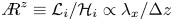 ${A{\kern-4pt}R} ^{z}\equiv \mathcal {L}_i/\mathcal {H}_i\propto \lambda _{x}/\Delta z$ and in the streamwise/spanwise plane
 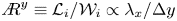 ${A{\kern-4pt}R} ^{y}\equiv \mathcal {L}_i/\mathcal {W}_i\propto \lambda _{x}/\Delta y$, respectively. Baars et al. (Reference Baars, Hutchins and Marusic2017) reported that in the neutral laboratory zero-pressure gradient TBL, the self-similarity is described by a streamwise/wall-normal aspect ratio
  $\lambda _{x}/\Delta z \approx 14$. A recent study by Baidya et al. (Reference Baidya2019), in high-Reynolds-number pipe and boundary layer flows, indicated that the self-similar wall-attached structures follow the three-dimensional aspect ratio 14 : 1 : 1 in the streamwise, spanwise and wall-normal directions, respectively. More recently, Krug et al. (Reference Krug, Baars, Hutchins and Marusic2019) explored the coherence for both velocity and temperature signals in the atmospheric surface layer (ASL). They found that the streamwise/wall-normal aspect ratio (
 ${A{\kern-4pt}R} ^{z} \equiv \lambda _x/\Delta z$) decays with a logarithmic trend with increasing unstable thermal stratification; spanwise information was not explored in their study. Moreover, they found that in the case of stable thermal stratification, the turbulence structures do not adhere to a self-similar scaling, meaning that an aspect ratio is not defined.
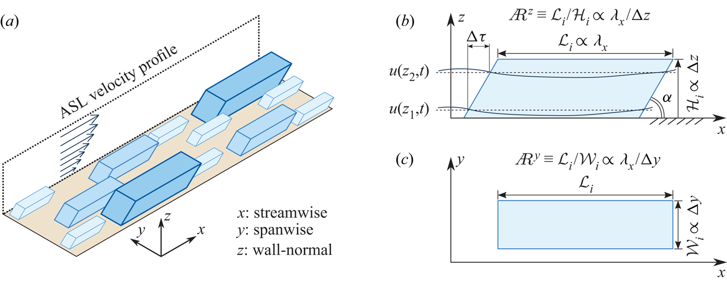
Figure 1. (a) Isometric view of three hierarchies of self-similar wall-attached eddies (simplified as slanted cuboids) in the logarithmic region of an ASL. The (b)  $x$,
$x$, $z$-plane and (c)
  $x$,
$x$, $y$-plane of one structure. Here,
  $\mathcal {L}_i$,
  $\mathcal {W}_i$ and
  $\mathcal {H}_i$ denote the streamwise, spanwise and wall-normal extents of the
  $i{\rm th}$ hierarchy structure.
Coherent structures reported in TBLs have been associated with characteristic inclination angles because of the mean shear. In the idealized (statistical) view of figure 1(b), inclination angle  $\alpha$ in the
  $x$,
$x$, $z$-plane reflects a phase shift
  $\Delta \tau$ in time series of velocity fluctuations at different
  $z$. Perry & Chong (Reference Perry and Chong1982) used a vortex skeleton approach and the Biot–Savart law to determine the inviscid velocity field of a representative eddy, termed the
  $\varLambda$-vortex. In neutral TBLs, hairpin vortices have been invoked commonly as the representative eddy, and Adrian, Meinhart & Tomkins (Reference Adrian, Meinhart and Tomkins2000) suggested that these vortices are arranged together in groups called vortex packets. (For a comprehensive review of hairpin structures and their generating mechanisms, see Adrian Reference Adrian2007.) Christensen & Adrian (Reference Christensen and Adrian2001) found that the sequence of individual vortex heads forms an interface or shear layer that is, statistically, inclined away from the wall at angles between
  $12^{\circ }$ and
  $20^{\circ }$. Laboratory results indicate the most probable inclination angle to be around
  $10^{\circ }$–
 $15^{\circ }$ (Adrian et al. Reference Adrian, Meinhart and Tomkins2000; Christensen & Adrian Reference Christensen and Adrian2001; Baars, Hutchins & Marusic Reference Baars, Hutchins and Marusic2016). In the neutral surface layer, inclination angles ranging from
  $10^{\circ }$ to
  $20^{\circ }$ have been reported (Boppe, Neu & Shuai Reference Boppe, Neu and Shuai1999; Carper & Porté-Agel Reference Carper and Porté-Agel2004; Chauhan et al. Reference Chauhan, Hutchins, Monty and Marusic2013; Liu, Bo & Liang Reference Liu, Bo and Liang2017). Also, Marusic & Heuer (Reference Marusic and Heuer2007) demonstrated the invariance of the inclination angle in wall-bounded flows with zero buoyancy (neutral conditions) over a wide range of Reynolds numbers through laboratory and field experiments. The discussion above pertains to the near-neutral case. However, in studies of the ASL, it has been observed that the inclination angle changes drastically under different stability conditions. The thermal stability of the ASL is generally characterized by the Monin–Obukhov stability parameter
  $z_s/L$ (Obukhov Reference Obukhov1946; Monin & Obukhov Reference Monin and Obukhov1954), where
  $L=-u_{\tau }^{3}{\bar {\theta }}/(\kappa {g}\overline {w\theta })$ is the Obukhov length,
  $\kappa =0.41$ is the von Kármán constant,
  $g$ is the gravitational acceleration, and
  $\overline {w\theta }$ is the surface heat flux, with
  $w$ and
  $\theta$ the fluctuating wall-normal velocity and temperature components,
  $\bar {\theta }$ the mean temperature,
  $u_{\tau }$ the friction velocity, and
  $z_s$ the reference height for evaluating this parameter. Many studies have observed that the inclination angle of coherent structures becomes steeper with increasing unstable thermal stratification (Chauhan et al. Reference Chauhan, Hutchins, Monty and Marusic2013; Liu et al. Reference Liu, Bo and Liang2017; Lotfy & Harun Reference Lotfy and Harun2018). In addition, Chauhan et al. (Reference Chauhan, Hutchins, Monty and Marusic2013) reported that for the case of stable stratification, the statistical inclination angle reduced below the typical values found for the near-neutral case. Recently, Salesky & Anderson (Reference Salesky and Anderson2020a) introduced an additional parameter to account for the loading and unloading of surface layer flux–gradient relations imposed by the passage of large-scale motions (LSMs). Meanwhile, Salesky & Anderson (Reference Salesky and Anderson2020b) developed a prognostic model for large-scale structures, where the inclination angle is the sum of the inclination angle observed in a neutrally stratified wall-bounded turbulent flow and the stability-dependent inclination angle of the wedge. Baars et al. (Reference Baars, Hutchins and Marusic2016) indicates that in the neutral case, and for all scales
  $\lambda _x/\delta > 0.5$, the coherent scales obey a virtually constant inclination angle. In unstable conditions in the atmosphere, positive buoyancy lifts the structure away from the surface, leading to an increase in the statistical inclination angle (as averaged across all scales; see Chauhan et al. Reference Chauhan, Hutchins, Monty and Marusic2013; Liu et al. Reference Liu, Bo and Liang2017). Now, in the unstable case, the dominance of buoyancy over shear is a function of wall-normal height, hence one expects the inclination angle to be scale-dependent.
Since the coherent structure in the ASL has a strong relationship with the stability parameter, this paper will address specifically the influence of stability on: (1) the streamwise/wall-normal aspect ratio  ${A{\kern-4pt}R} ^{z}\equiv \lambda _{x}/\Delta z$ and the streamwise/spanwise aspect ratio
  ${A{\kern-4pt}R} ^{y}\equiv \lambda _{x}/\Delta y$ in § 3.1, and (2) the scale-dependent angle
  $\alpha$ in § 3.2, particularly under unstable conditions. Statistical relations for the aspect ratio and inclination angle for coherent turbulence fluctuations in the ASL are particularly relevant when analysing wind loading in the field of wind engineering (see Davenport Reference Davenport1961, Reference Davenport2002).
2. Turbulence dataset of the atmospheric surface layer
2.1. QLOA facility and available data
The measurement data used throughout this article were acquired at the QLOA facility in western China, Gansu province, during three-month long measurement campaigns over two years (March to May in 2014 and 2015). The QLOA consists of wall-normal and spanwise arrays of sonic anemometers, performing synchronous measurements of the three-dimensional turbulent flow field. Sonic anemometers (Gill Instruments R3-50 installed from  $s_2$ to
  $s_7$, and Campbell CSAT3B installed from
  $h_1$ to
  $h_{11}$; see figure 2) were employed to acquire time series data of the three components of velocity, as well as the air temperature, at a sampling frequency of 50 Hz. Continuous observations were conducted at the QLOA site for a duration of more than 3000 h, from which 89 h of data were selected to analyse the characteristics of the large-scale coherent structures under different stratification stability conditions. The wall-normal array consists of 11 sonic anemometers that were placed with a logarithmic spacing on a vertical radio-type tower. The spanwise array covered an overall distance of 30 m, with 7 anemometers that were placed at constant height (
 $z = 5$ m), with an equidistant spanwise spacing of 5 m. The spanwise and wall-normal coordinates for each of the 17 anemometers are provided in figure 2(b). It should be noted that the first sonic anemometer in the spanwise array (
 $s_1$) also functions as the fifth on the main tower (
 $h_5$), which means that we have 7 available anemometers in the spanwise array. The friction velocity
  $u_{\tau }$ is inferred from
  $u_{\tau }=(-\overline {uw})^{1/2}$ at
  $z = 5$ m (calculated by the mean value from 7 sonic anemometers in the spanwise array). We assume an estimate for the surface layer thickness of
  $\delta = 60$ m, following Hutchins et al. (Reference Hutchins, Chauhan, Marusic, Monty and Klewicki2012). The 89 h of data remaining after preselection were subdivided into 89 segments of 1 h long time series. This database included 69 h of unstable data (
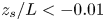 $z_s/L<-0.01$), 10 h of near-neutral data (
 $-0.01\leqslant z_s/L<0.01$), and 10 h of stable data (
 $z_s/L>0.01$). Recall that
  $z_s$ is the reference height used to define the stability parameter
  $z_{s}/L$. For the benefit of comparison with previous works (Chauhan et al. Reference Chauhan, Hutchins, Monty and Marusic2013; Liu et al. Reference Liu, Bo and Liang2017; Krug et al. Reference Krug, Baars, Hutchins and Marusic2019), the majority of our work uses
  $z_s = 2.5$ m, unless otherwise specified. The demarcation of
  $z_s/L = -0.01$ to distinguish between neutral and unstable thermal stratification is found commonly in the literature, but for all analysis in this paper, we present results as a function of
  $z_s/L$; it will actually be shown later that this demarcation of
  $z_s/L = -0.01$ is too permissive. The preselection criteria included wind direction (the wind direction had to be aligned with the
  $x$ axis of the anemometer to within
  ${\pm }30^{\circ }$) and steadiness (statistically steady conditions based on the high-quality requirement by Foken et al. Reference Foken, Göockede, Mauder, Mahrt, Amiro and Munger2005). A de-trending operation is also added (to remove the large-scale synoptic trend). See Hutchins et al. (Reference Hutchins, Chauhan, Marusic, Monty and Klewicki2012) and Wang & Zheng (Reference Wang and Zheng2016) for full details of the preselection criteria.
Figure 2. (a) Three-dimensional view of the measurement set-up at the QLOA site. (b) North-west view of the sonic anemometer array; Campbell CSAT3B and Gill Instruments R3-50 sonics were installed at positions  $h_1$ to
  $h_{11}$ and
  $s_2$ to
  $s_7$, respectively.
2.2. Processing method
Two-point correlations can be computed on a per-scale basis in the Fourier domain using the linear coherence spectrum (LCS). For the fluctuating streamwise velocity signals  $u$, the LCS is defined as
 \begin{equation} \gamma_{L}^{2}(z,z_{ ref};\lambda_{x})\equiv\frac{|\langle{\tilde{U}(z;\lambda_{x})\,\tilde{U}^{*}(z_{ ref};\lambda_{x})}\rangle|^{2}}{\langle{|\tilde{U}(z;\lambda_{x})|^{2}}\rangle\langle{|\tilde{U}(z_{ ref};\lambda_{x})|^{2}}\rangle}=\frac{|\phi_{uu}^{\prime}(z,z_{ ref};\lambda_{x})|^{2}}{\phi_{uu}(z;\lambda_{x})\,\phi_{uu}(z_{ ref};\lambda_{x})}. \end{equation}
Here,  $\tilde {U}(z;\lambda _{x})=\mathcal {F}[u(z)]$ is the Fourier transform of
  $u(z)$, in either
  $x$ or time. The spatio-temporal transformation uses Taylor's hypothesis (Taylor Reference Taylor1938), where the local mean velocity is taken as the convection velocity. The asterisk
  $*$ indicates the complex conjugate,
  $\langle \rangle$ denotes ensemble averaging, and
  $|~|$ designates the modulus. Scale-dependent phase information is embedded explicitly in the phase of the cross-spectrum
  $\phi _{uu}^{\prime }$. For (2.1), the LCS is defined based on
  $u$ at two positions (
 $z_{ref}$ and
  $z$), separated in the wall-normal direction by
  $\Delta z \equiv z - z_{ref}$. This coherence can also be computed across all other measured signals (
 $v$ and
  $\theta$) and also across spanwise separations
  $\Delta y$. The reference signal's height is denoted with the subscript ‘ref’ and is thus stated as
  $z_{ref}$. Since the LCS considers the magnitude of the complex-valued cross-spectrum, only the magnitude of coherence is considered (phase is covered later). Based on assumptions from the AEH (Baars et al. Reference Baars, Hutchins and Marusic2017; Krug et al. Reference Krug, Baars, Hutchins and Marusic2019), the coherence magnitude within a self-similar region in
  $\lambda _x$,
 $z$-space is expected to adhere to
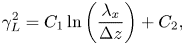 \begin{equation} \gamma_{L}^{2}=C_1\ln\left( \frac{\lambda_{x}}{\Delta z} \right) +C_{2}, \end{equation}
from which the statistical aspect ratio (in this case streamwise/wall-normal) then follows:
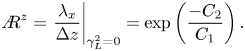 \begin{equation} {A{\kern-4pt}R}^{z} = \left. \frac{\lambda_x}{\Delta z}\right\vert_{\gamma_{L}^{2}=0}=\exp\left(\frac{-C_{2}}{C_{1}} \right). \end{equation}
Here,  $C_1$ and
  $C_2$ are fitted parameters. Figure 3 shows an example of data obtained from the ASL to illustrate the process of the coherence spectrum. Figure 3(a) indicates the raw data for the streamwise velocity collected at
  $h_5 = 5$ m and
  $h_6 = 7.15$ m, under unstable conditions with
  $z_{s}/L=-0.52$. A shorter time history of corresponding filtered signals is shown in figure 3(b), evidencing that signal
  $h_6$ leads
  $h_5$. Thus a coherent velocity fluctuation is first sensed at the higher wall-normal location as a result of the structure inclination angle. The LCS for
  $h_5$ and
  $h_6$ is presented in figure 3(c) as a function of temporal frequency, as computed from the 1 h long time series data. Using Taylor's frozen turbulence hypothesis, the frequency axis can be converted to a streamwise wavelength:
  $\lambda _x \equiv U_c/f$. Here,
  $U_{c}$ is a convective speed, taken as the mean velocity at local height
  $z$. (The current dataset is fully submerged in the logarithmic region of the ASL. Here, the convective speed of coherent structures agrees well with the mean velocity and is relatively scale-independent (Liu & Gayme Reference Liu and Gayme2020). Moreover, Baars et al. (Reference Baars, Hutchins and Marusic2017) showed that when Taylor's hypothesis is used with the local mean velocity
  $U(z)$, the coherence spectra agree with those computed from spatial DNS data.) The coherence spectrum of figure 3(c) can now be presented as a function of the streamwise wavelength, relative to the wall-normal separation distance
  $\Delta z$, as shown in figure 3(d). In addition to the coherence spectrum for
  $h_5$ and
  $h_6$, the coherence spectra for all heights above
  $h_6$ (relative to
  $h_5$ again) are also shown to illustrate the wall-similarity that is to be investigated. Krug et al. (Reference Krug, Baars, Hutchins and Marusic2019) noticed that only data at neutral and unstable thermal stratification conditions complied with (2.2), thus an aspect ratio was found only for those conditions. (A similar conclusion was reached for our QLOA site data, therefore we do not consider stable stratification with
  $z_s/L > 0$.) In addition, Krug et al. (Reference Krug, Baars, Hutchins and Marusic2019) found that the self-similar scaling applies also to fluctuations of the spanwise velocity
  $v$ and the static temperature
  $\theta$. Baidya et al. (Reference Baidya2019) demonstrated that a scaling similar to (2.2) and (2.3) occurs in the spanwise direction, resulting in a streamwise/spanwise aspect ratio
  ${A{\kern-4pt}R} ^{y}$ for the self-similar structure.
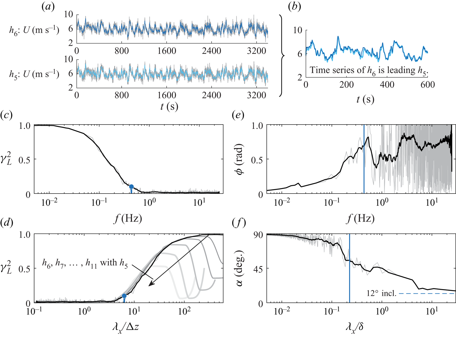
Figure 3. (a) An example of time series data for  $z_s/L = -0.52$ at heights
  $h_5$ and
  $h_6$. The blue lines are low-pass filtered at
  $f = U/\delta$. (b) Portion of the filtered signals for inspecting the coherence and time shift. (c) Coherence spectrum for height
  $h_6$, relative to
  $h_5$, as a function of temporal frequency. (d) Coherence spectrum for all heights
  $h_6,\ldots,h_{11}$, again relative to
  $h_5$. Here, the abscissa is converted to a spatial wavelength with the mean velocity at height
  $z$. (e) Scale-dependent phase of the cross-spectrum between
  $h_5$ and
  $h_6$, which is converted to a physical inclination angle
  $\alpha$ as a function of a spatial wavelength in (f). The blue dots and blue solid lines in (c–f) indicate the frequency or wavelength corresponding to
  $\gamma _L^{2}=0.1$. Filtered spectra (black line), overlaid on the grey raw spectra, utilize a bandwidth moving filter of 25 %.
Scale-dependent phase information is embedded explicitly in the phase of the cross-spectrum  $\phi _{uu}^{\prime }$, given by
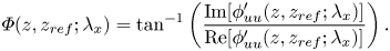 \begin{equation} \varPhi(z,z_{ref};\lambda_x)= \tan^{{-}1}\left(\frac{{\rm Im} [\phi_{uu}^{\prime}(z,z_{ref};\lambda_x) ]}{{\rm Re}[\phi_{uu}^{\prime}(z,z_{ref};\lambda_x)]}\right). \end{equation}
The phase spectrum aids in assessing the temporal shift between signals. Phase  $\varPhi (f)$ in (2.4) is shown in figure 3(e) and can be used to extract a scale-by-scale inclination angle
  $\alpha$ (as shown in figure 3f). That is, the temporal shift is
 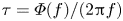 $\tau =\varPhi (f)/(2{\rm \pi} {f})$, where
  $f$ is the mode frequency, and aids in computing the physical inclination angle through
 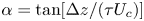 $\alpha =\tan [\Delta z/(\tau U_{c})]$. For the spectral analysis, the highest frequency resolved is set by the Nyquist frequency
  $f_s/2 = 25$ Hz, where
  $f_s = 50$ Hz is the sampling frequency. The lowest frequency is dictated by the interval length
  $I$ used in the spectral analysis, and the longest interval used was
  $I = 2^{N}$ samples with
  $N = 15$ (interval length
  ${\approx }650$ s). A composite approach with varying interval length (
 $N = 8,\ldots,15$) was used to generate the full spectra with as many ensembles as possible for the higher frequency portions of the spectrum (for
  $N = 8$ a total of around 1000 ensembles were used).
3. Results
3.1. Stability dependence of aspect ratio
The linear coherence spectra for  $u$,
$u$,  $v$ and
  $\theta$ as functions of
  $\lambda _x/\Delta z$ and
  $\lambda _x/\Delta y$ for the unstable case with
  $z_s/L = -0.52$ are given in figures 4(a) and 4(c), respectively. As reported by Krug et al. (Reference Krug, Baars, Hutchins and Marusic2019), the LCS collapses on one common curve over a range of
  $\lambda _x/\Delta z$ and
  $\lambda _x/\Delta y$. By fitting (2.2) to these regions to obtain
  $C_1$ and
  $C_2$, the aspect ratio
  ${A{\kern-4pt}R}$ can be assessed. For this particular unstable case, we might expect the positive buoyancy to cause the self-similar structures in the hierarchy to lift more aggressively from the wall, extending the wall-normal coherence for a given
  $\lambda _x$ scale, hence reducing
  ${A{\kern-4pt}R} ^{z}_u$. Indeed, for the unstable case considered in figure 4(a), this yields an
  ${A{\kern-4pt}R} _u^{z}$ that is significantly lower (
 ${A{\kern-4pt}R} ^{z}_{u}= 3.6$) than the value
  ${A{\kern-4pt}R} ^{z}_{u}\approx 14$ reported for laboratory neutral conditions (Baars et al. Reference Baars, Hutchins and Marusic2017) and in close agreement with the aspect ratio reported in Krug et al. (Reference Krug, Baars, Hutchins and Marusic2019) for similar values of the stability parameter. The resulting aspect ratios for
  $u$,
$u$,  $v$ and
  $\theta$ from all 79 h datasets (covering a range of stabilities from
 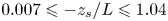 $0.007 \leqslant -z_{s}/L \leqslant 1.04$) are plotted as functions of the stability parameter in figure 4(b) for streamwise/wall-normal aspect ratios
  ${A{\kern-4pt}R} ^{z}$, and in figure 4(d) for streamwise/spanwise aspect ratios
  ${A{\kern-4pt}R} ^{y}$. In all cases, a clear trend emerges between aspect ratio and stability parameter, and a log–linear trend is fitted to the extracted data (black solid curves). These fitted trends are consistent with those of Krug et al. (Reference Krug, Baars, Hutchins and Marusic2019) (black dashed curves in figure 4b), indicating that the self-similar scaling under near-neutral and unstable conditions is a universal phenomenon. The relatively small differences in the slopes of the solid (current study) and dashed (Krug et al. Reference Krug, Baars, Hutchins and Marusic2019) trend lines, visible in particular for
  ${A{\kern-4pt}R} ^{z}_{u}$ and
  ${A{\kern-4pt}R} ^{z}_{\theta }$, are ascribed to experimental uncertainty in the field measurements: e.g. differences between test sites and the fact that the fitting procedure was performed on a different number of data points, residing at different values of
  $-z_s/L$. As an extension to the results of Krug et al. (Reference Krug, Baars, Hutchins and Marusic2019), the streamwise/spanwise aspect ratios of figure 4(d) seem to also exhibit log–linear trends, although in these cases the scatter in results is greater.
Figure 4. Plots of  $\gamma ^{2}_L$ in the ranges
  $2.15\ {\rm m} \leqslant \Delta z \leqslant 25$ m and
  $5\ {\rm m} \leqslant \Delta y \leqslant 30$ m (with increasing
  $\Delta z$ and
  $\Delta y$ indicated by lighter shades of grey) for (a) the wall-normal coordinate
  $z$, and (c) the spanwise coordinate
  $y$, respectively, for the unstable case with
  $z_s/L = -0.52$. Here, the ranges are between
  $\Delta z_{5,6} = h_6 - h_5 = 2.15\ {\rm m}$ and
  $\Delta z_{5,11} = h_{11} - h_5 = 25$ m, and between
  $\Delta y_{1,2} = s_2 - s_1 = 5$ m and
  $\Delta y_{1,7} = s_7-s_1 = 30$ m. The blue line is a fit to obtain the aspect ratio according to (2.2), with
  $C_{1}=0.302$ fixed; the fitting region used is bounded by
  $\gamma _{L}^{2}>0.1$ and
  $\lambda _x < 100$ m, and is indicated by red lines. Subscript
  $i=u,v,\theta$ in
  ${A{\kern-4pt}R} _{i}^{k}$ signifies the aspect ratio for streamwise and spanwise velocity components as well as the temperature component; superscript
  $k=z,y$ in A
 $_{i}^{k}$ indicates either the streamwise/wall-normal or streamwise/spanwise aspect ratio. (b,d) Streamwise/wall-normal and streamwise/spanwise aspect ratios, respectively, as functions of
  $z_s/L$. The blue dots are our ASL results, and the black solid lines denote the semi-log fitting. The dashed lines in (b) come from Krug et al. (Reference Krug, Baars, Hutchins and Marusic2019) with
  $z_{s}=2.14$ m and
  $z_{ ref}=1.41$ m. Note that in this work,
  $z_{ref}=z_s=5$ m, so the dashed lines of Krug et al. (Reference Krug, Baars, Hutchins and Marusic2019) were shifted along the
  $z_s$ axis to compare the trends at matched
  $-z_s/L$.
Baidya et al. (Reference Baidya2019) indicates that the aspect ratio is  ${A{\kern-4pt}R} ^{z}_{u}:{A{\kern-4pt}R} ^{y}_{u}=1:1$ in the laboratory neutral condition. The results shown in figures 4(b,d) are also supportive of this. For instance, by utilizing the solid trend lines in figures 4(b,d), for
  ${A{\kern-4pt}R} _u^{z}$ and
  ${A{\kern-4pt}R} _u^{y}$, respectively, it is found that
  ${A{\kern-4pt}R} _u^{z}:{A{\kern-4pt}R} _u^{y} = 0.90:1$ for the near-neutral case
  $z_s/L = -0.01$, and that this ratio changes to
  ${A{\kern-4pt}R} _u^{z}:{A{\kern-4pt}R} _u^{y} = 1:1$ for a strong unstable stability condition
  $z_s/L = -1$. By recalling that
  ${A{\kern-4pt}R} _u^{z} \equiv \lambda _x/\Delta z$, the data here indicate that these self-similar eddies for
  $u$ follow an aspect ratio
  $\lambda _x:\Delta y:\Delta {z} \approx 6.4:0.90:1$ in the near-neutral condition (
 $z_s/L = -0.01$). It is worth highlighting that again the aspect ratio is sensitive to even very weakly unstable conditions. Therefore, the value for
  $u$ measured in the ASL is less than the result
  $\lambda _x/\Delta z = 14$ from Baars et al. (Reference Baars, Hutchins and Marusic2017) and Baidya et al. (Reference Baidya2019) in neutral laboratory conditions, as was also noticed by Krug et al. (Reference Krug, Baars, Hutchins and Marusic2019), whose prediction implies that
  $\lambda _x/\Delta z = 14$ will be attained only for
  $\vert z_s/L \vert \approx 0.0003$ (but for the current QLOA dataset, we have data only for
  $\vert z_s/L \vert \geqslant 0.007$). Finally, the aspect ratio for
  $u$ shows that
 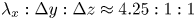 $\lambda _x:\Delta y:\Delta z\approx 4.25:1:1$ under a more unstable condition (
 $z_s/L = -1$), demonstrating that positive buoyancy has a lifting effect, increasing the size of coherent structures in the wall-normal and spanwise directions relative to its streamwise extent.
3.2. Stability dependence of structure inclination angle
Per the phase spectrum in figure 3(f), the scale-dependent phase is now analysed for scales within the range  $1 < \lambda _x/\delta < 10$ and for a similar
  $\Delta z$ as before,
  $\Delta z = h_5 - h_1 = 4.1$ m. Larger wavelength information in the phase spectra is prone to noise issues due to the limited ensembles available for constructing the spectra, while smaller wavelengths generally have a lower coherence. Figure 5(a) indicates the phase spectra in terms of inclination angle as functions of wavelength
  $\lambda _x/\delta$, for all different stability parameters
  $-z_s/L$. Note that all measured angles in figure 5(a) are positive, corresponding to forward-leaning structures. Though there are some clear outliers in these plots, certain trends are visible, as evidenced by the coloured symbols that visualize data at constant scales
  $\lambda _x/\delta = 1$, 2 and 6. Clearly, these different wavelengths exhibit different dependencies of
  $\alpha$ with the stability parameter, with
  $\lambda _x/\delta = 1$ exhibiting much steeper angles
  $\alpha$ in the most unstable cases, and markedly shallower angles as near-neutrality is approached. In general, it is also noted that longer structures (larger wavelength) will exhibit smaller inclination angles, especially noticeable at stronger convective conditions.
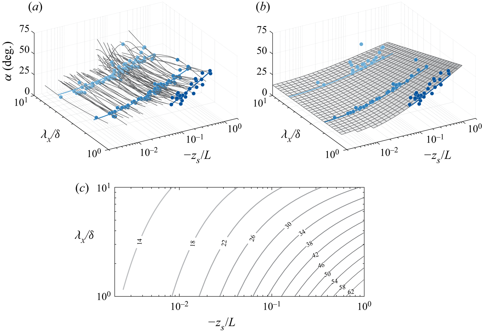
Figure 5. (a) The phase expressed as a physical inclination angle  $\alpha$ as a function of wavelength
  $\lambda _{x}/\delta$ and stability parameter
  $-z_s/L$. The LCS reference height,
  $z_{ref}=0.90$ m, and inclination angles are presented for distances
  $\Delta z = h_5 - h_1 = 4.1$ m. The solid increasing shades of blue dots indicate the scales at
  $\lambda _{x}/\delta =1$,
  $\lambda _{x}/\delta =2$ and
  $\lambda _{x}/\delta =6$, addressed in detail in figure 6. The solid blue lines show the trend fitted to these data given by (b) the surface fit to the data of the form (3.1). (c) Similar to (b), but now as two-dimensional iso-contours of
  $\alpha$ as a function of
  $\lambda _{x}/\delta$ and
  $-z_s/L$.
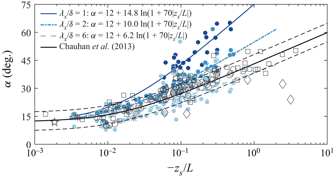
Figure 6. Variation of  $\alpha$ with the stability parameter
  $z_s/L$ (
 $z_s = 2.5$ m,
  $z_{ref} = 0.90$ m and
  $z = 5$ m, so that
  $\Delta z = 4.1$ m). The solid coloured lines are the fitting lines based on (3.1) for the corresponding scales
  $\lambda _x/\delta = 1$, 2 and 6. Current data are shown by black circles (based on a two-point correlation, including all scales). The open black squares correspond to near-neutral and unstable ASL data of Chauhan et al. (Reference Chauhan, Hutchins, Monty and Marusic2013); asterisks from
  $R_{u_{\tau }u}$ of Marusic & Heuer (Reference Marusic and Heuer2007); diamonds of Carper & Porté-Agel (Reference Carper and Porté-Agel2004); open pentagram from
  $R_{uu}$ of Marusic & Heuer (Reference Marusic and Heuer2007).
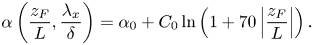
To quantify the trends in the data, a functional form is adopted from Chauhan et al. (Reference Chauhan, Hutchins, Monty and Marusic2013), who used a log–linear trend of convective data in a boundary layer to model the variation of  $\alpha$ with stability
  $z_s/L$. Note that their angle was inferred from two-point cross-correlation maps and hence is scale-invariant. As such, the only difference is the introduction of a scale-dependent coefficient, here denoted as
  $C_0 = C_0(\lambda _x/\delta )$ in (3.1). This function will be illustrated later, but can capture the faster increase of
  $\alpha$ with increasing
  $-z_s/L$, for smaller scales. (In the work of Chauhan et al. (Reference Chauhan, Hutchins, Monty and Marusic2013) this coefficient was constant and equaled
  $C_0 = 7.3$.) So we have
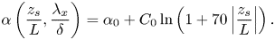 \begin{equation} \alpha \left(\frac{z_s}{L},\frac{\lambda_x}{\delta}\right) =\alpha_{0}+C_0\ln \left(1 + 70\left\vert \frac{z_s}{L} \right\vert \right). \end{equation}
The form of (3.1) guarantees that  $\alpha$ approaches the invariant value of
  $\alpha _0$ when
  $-z_s/L \rightarrow 0$ (here,
  $\alpha _0$ is taken as
  $12^{\circ }$, and recall that
  $z_s = 2.5$ m). A curve-fitted plane to those spectra is shown in figure 5(b), in which this fit has the form in (3.1); iso-contours of
  $\alpha$ are depicted in figure 5(c), and show that under the most unstable conditions, coherent structures of
  $\lambda _x/\delta = 1$ are inclined at angles as high as
  $65^{\circ }$. It should be noted from figure 5(a) that for small near-neutral values of the stability parameter, it is not always possible to compute an inclination angle
  $\alpha$ for the smaller wavelength (
 $\lambda _x/\delta = 1$) from the phase spectra since the coherence across
  $\Delta z$ drops below
  $\gamma _L^{2} = 0.1$.
Figure 6 shows the variation of  $\alpha$ as a function of the stability parameter
  $-z_s/L$ for three different length scales,
  $\lambda _x/\delta = 1,2,6$. Inclination angles computed from the phase spectra are shown by the coloured circles, and the blue lines show the surface fit to the data given by (3.1). In addition, the black open circles in figure 6, which show the inclination computed from the two-point correlations for all 11 measurement heights, indicate that the current data are consistent with the similarly computed results from Chauhan et al. (Reference Chauhan, Hutchins, Monty and Marusic2013), shown by the black open squares. The black solid line in figure 6 shows the fit proposed by Chauhan et al. (Reference Chauhan, Hutchins, Monty and Marusic2013) based on the two-point correlation contours. As such, this original fit includes all scales, and is skewed disproportionately towards larger-scale features at higher
  $z$. It is clear from figure 6 that the increasing buoyancy lifts all scales to larger inclination angles, although the smaller-scale structures considered (
 $\lambda _x/\delta = 1$) exhibit steeper angles at all values of the stability parameter as compared to the larger features (
 $\lambda _x / \delta = 6$). This means that the scale-dependent coefficient
  $C_0 = C_0(\lambda _x/\delta )$ in (3.1) increases systematically as we focus on smaller scales. The coloured curves in figure 6 show the curve fits to the data based on the fit proposed in (3.1), with the constant
  $\alpha _0$ and value of the scale-dependent coefficient
  $C_0$ given in the figure legend. It should be noted here that for the limited scale range discussed here,
  $1 < \lambda _x/\delta < 10$, all of these scales are large and associated with the upper end of attached motions and superstructures (Hutchins & Marusic Reference Hutchins and Marusic2007). Although with increasing stability all scales are lifted compared with the neutral condition, the low end of this range (
 $\lambda _x/\delta = 1$) exhibits the steepest angles, reaching
  $\alpha \approx 70^{\circ }$ at
  $z_s/L= -1.0$. Baars et al. (Reference Baars, Hutchins and Marusic2016) indicated that the inclination angle of the large-scale structures in the neutral laboratory boundary layer is scale-independent with value
  $\alpha = 14.7^{\circ }$. Though the data in figure 6 do suggest that
  $\alpha$ becomes scale-independent in the limit of small
  $\vert z_s/L \vert$, the angle seems to be closer to
  $\alpha \approx 12^{\circ }$ for the current data.
The results summarized in figure 6 are computed for a linear coherence spectrum between the reference location  $z_{ref} = 0.9$ m and the location
  $z = 5$ m (
 $\Delta z = 4.1$ m). In addition, the stability parameter presented on the abscissa of figure 6 is computed based on conditions at
  $z_s = 2.5$ m. Before considering further the form of the fit described by (3.1), we must consider the sensitivity to
  $z_s$, and
  $\Delta z$. Generally, the stability parameter
  $z_s/L$ depends linearly on height, which would suggest that the scale-dependent structure inclination angles
  $\alpha$ will also increase with wall-normal height
  $z$ (since as we move away from the wall, buoyancy effects will increase in dominance relative to shear). To account for this, and to form a stability parameter that better reflects the altitude at which the phase spectrum is evaluated, we propose a fractional stability parameter, dubbed
  $z_F/L$, where
  $z_F$ is fixed at a constant fraction of the wall-normal offset
  $\Delta z$. Hence stability is always assessed at a fixed fractional height between the lower and upper probes used to compute the linear coherence spectrum. This should minimize the sensitivity of the inclination angle–stability parameter relationship to changes in
  $\Delta z$. Since the data in figure 6 are given based on
  $z_{ref} = 0.90$ m,
  $z = 5$ m and
  $z_s = 2.5$ m (figure 7), the fractional stability parameter
  $z_F$ can be assessed as
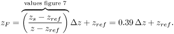 \begin{equation} z_F = \overbrace{\left(\frac{z_s-z_{ref}}{z-z_{ref}}\right)}^{\text{values figure~7}}\Delta z+z_{ref} = 0.39\,\Delta z + z_{ref}. \end{equation}
Maintaining  $z_F$ at the value given by (3.2), when changing
  $\Delta z$ or
  $z_{ref}$, ensures that we assess stability at the same fractional location
  $0.39\,\Delta z$ when varying the height of inspection
  $z$. We can now substitute
  $z_F$ for
  $z_s$ in (3.1):
 \begin{equation} \alpha\left(\frac{z_F}{L},\frac{\lambda_{x}}{\delta}\right) =\alpha_{0}+C_{0} \ln\left(1+70\left\vert\frac{z_F}{L}\right\vert \right). \end{equation}
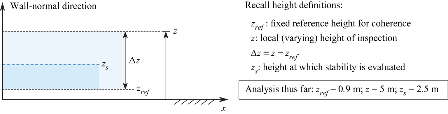
Figure 7. Summary of the different heights involved in the analysis. Heights for which the analyses were performed up to this point are listed in the box.
The grey curves in figure 8(a) show coefficient 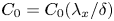 $C_0 = C_0(\lambda _x/\delta )$ from (3.3), extracted from fits to the data with various
  $\Delta z$. Here,
  $z_{ref}$ remains fixed at 0.90 m, and
  $z$ covers all heights above, ranging from 1.71 m to 30 m, with thinner grey lines indicating lower values of
  $z$. We can extract
  $\alpha$ from the phase spectra only in situations where the coherence
  $\gamma _L^{2}$ is greater than 0.1; this condition gives rise to the sharp drops/rises in figure 8(a) as at different
  $\lambda _x/\delta$, varying subsets of data are available for the calculation of
  $\alpha$. In general, it is noted that the fractional location for the stability height described above does a reasonable job of collapsing the
  $C_0$ curves for all
  $\Delta z$;
  $C_0$ decreases with
  $\lambda _x/\delta$, indicating that the smaller-scale structures tend to have larger inclination angles in the convective conditions. Based on the approximate collapse observed in figure 8(a), we can approximate crudely the
  $\lambda _x/\delta$ dependence of
  $C_0$ with
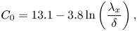 \begin{equation} C_{0}=13.1-3.8\ln\left(\frac{\lambda_x}{\delta}\right), \end{equation}
which is shown by the blue solid line in figure 8(a). Finally, by combining (3.4) with (3.3), we obtain the scale-dependent structural inclination angle as
 \begin{equation} \alpha\left(\frac{z_F}{L},\frac{\lambda_{x}}{\delta}\right) =\alpha_{0}+\left(13.1-3.8\ln\left(\frac{\lambda_{x}}{\delta}\right)\right)\ln\left(1+70\left|\frac{z_F}{L}\right|\right). \end{equation}
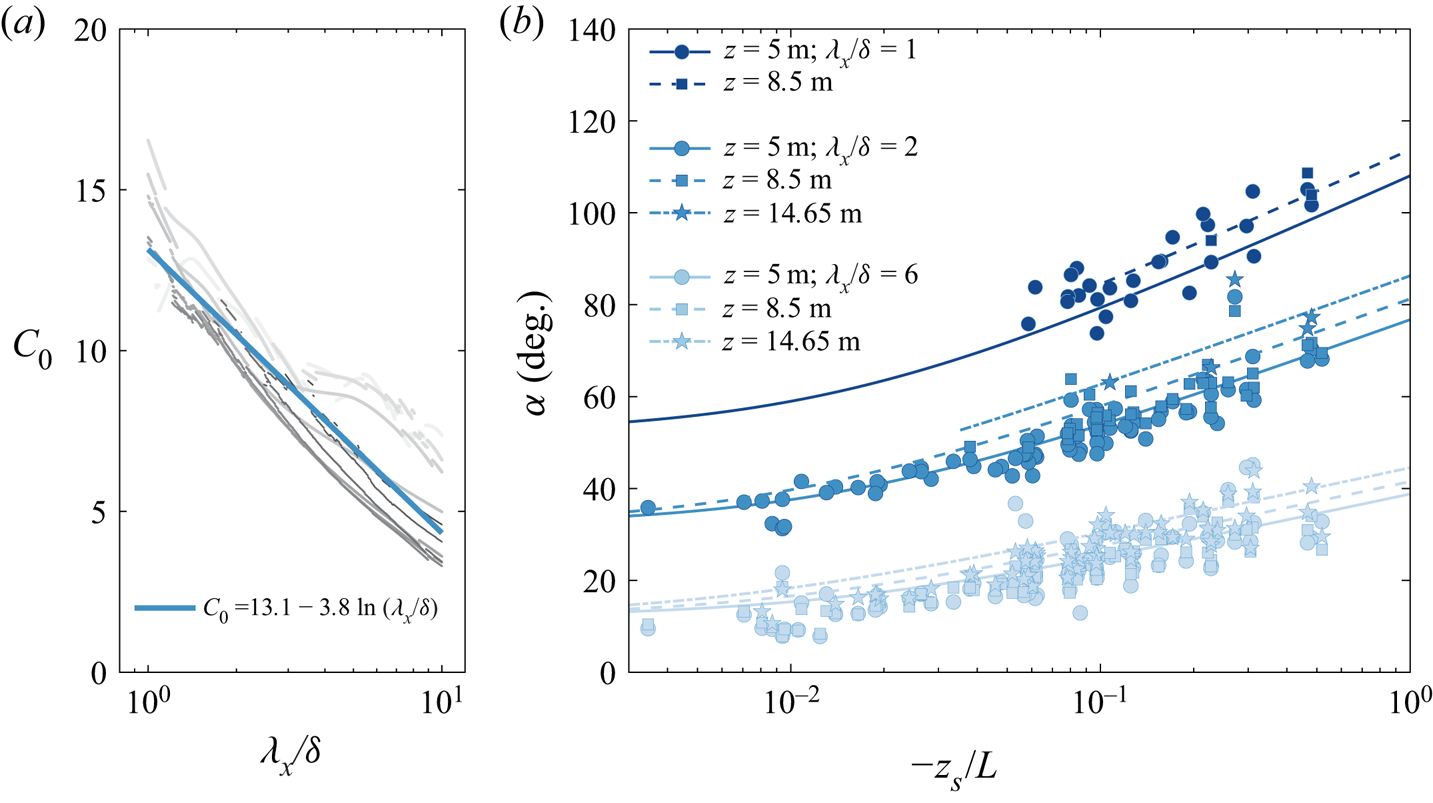
Figure 8. (a) Parameter  $C_{0}$ as a function of wavelength
  $\lambda _x$ with increasing
  $\Delta z$ indicated by thinner lines and darker shades of grey. Here,
  $z_{ref}$ remains fixed at
  $h_1 = 0.91$ m, and
  $z$ increases from 1.71 m to 30 m (
 $h_2$ to
  $h_{11}$); the blue solid line indicates a log–linear fit to all grey curves. (b) The scale-dependent
  $\alpha$ for
  $u$ as a function of stability parameter, for
  $\lambda _x/\delta =1,2,6$ at
  $h_5$,
  $h_7$ and
  $h_9$ (
 $z_s = 2.5$ m and
  $z_{ref} = 0.90$ m); lines come from (3.5), and each set of profiles is offset by
  $15^{\circ }$.
Figure 8(b) shows the influence of wall-normal offset  $\Delta z$ (with
  $z_{ref}$ fixed at 0.90 m) on the computed inclination angle
  $\alpha$ as a function of stability for the wavelengths
  $\lambda _{x}/\delta =1,2,6$ for
  $u$. A larger
  $\Delta z$ leads to higher
  $\alpha$, but this can be accounted for by considering the fractional stability parameter. The curves, showing (3.5), describe the variation of
  $\alpha$ with
  $z_s/L$,
  $\lambda _x/\delta$ and
  $\Delta z$ reasonably well.
By way of a summary, figure 9 shows an illustration of the scale-dependent structure inclination angle and aspect ratio for both neutral (subscript  $n$) and unstable (subscript
  $u$) thermal stratification conditions. The illustrations show the streamwise extent of the structure (in physical space following the simplification that its length
  $\mathcal {L}$ scales with half the wavelength, thus
  $\mathcal {L} \sim \lambda _x/2$) and its wall-normal extent with height
  $\mathcal {H}$; the streamwise/wall-normal aspect ratio of the structure in the
  $x$,
$x$, $z$-plane adheres to
  ${A{\kern-4pt}R} _u^{z}$ of figure 4(b). When concentrating on the neutral stability condition first (bottom part of figure 9), both scales drawn exhibit the same inclination angle
  $\alpha _n$. That is, the statistical inclination angles of large and small scale comprise the same forward leaning behaviour.
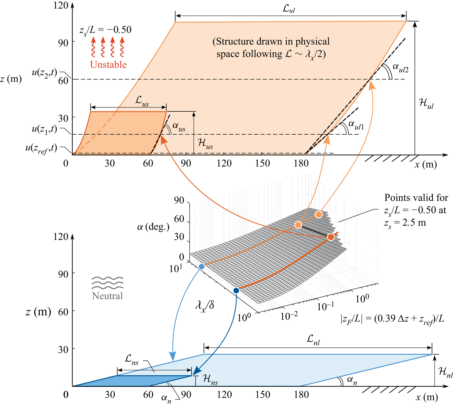
Figure 9. Summary of aspect ratio  ${A{\kern-4pt}R} ^{z}$ and scale-dependent angle
  $\alpha$ in a neutral and unstable stratified ASL. Two hierarchy levels are considered, each of a different scale:
  $\mathcal {L}$ and
  $\mathcal {H}$ show the structure's streamwise length and wall-normal height. The subscripts’ first letter,
  $n$ or
  $u$, signifies a ‘neutral’ or ‘unstable’ condition, and the second designation,
  $s$ or
  $l$, denotes ‘small-scale’ (
 $\lambda _x/\delta = 2$) or ‘large-scale’ (
 $\lambda _x/\delta = 6$). The dashed lines in the top part indicate a reference location
  $z_{ref} = 0.90$ m and heights
 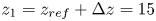 $z_1 = z_{ref} + \Delta z = 15$ m and
 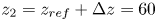 $z_2 = z_{ref} + \Delta z = 60$ m, for which the corresponding
  $\alpha$ values are indicated.
When considering unstable thermal stratification – in figure 9, just one value of  $z_s/L = -0.50$ is considered, evaluated at
  $z_s = 2.5$ m – the inclination angle is scale-dependent and also varies with
  $z$ (the procedure for plotting this structure is summarized in the Appendix). First, note that the coherent wall-attached structures are still self-similar per the definition used in this paper, based on the structure's streamwise wavelength relative to its wall-normal extent. But the aspect ratio reduces compared to the neutral case, and this depends on the degree of thermal stratification per the relations shown in figure 4(b), thus
  $(\mathcal {L}_{ns}/\mathcal {H}_{ns} = \mathcal {L}_{nl}/\mathcal {H}_{nl}) > (\mathcal {L}_{us}/\mathcal {H}_{us} = \mathcal {L}_{ul}/\mathcal {H}_{ul})$. Here, subscripts
  $s$ and
  $l$ refer to the small- and large-scale structures visualized, respectively. Concentrating on the inclination angle (e.g. the phase shift between a reference height
  $z_{ref}$ and a height of inspection
  $z$), it was found that for unstable stratification, it increases with increasing
  $z$. Hence
  $\alpha _{ul2} > \alpha _{ul1}$, and the coherent shape of the structure is characterized by a leading/trailing edge front that is curved and becomes steeper with height. Moreover, smaller-scale structures exhibit steeper angles for the case of equal
  $\Delta z$ (e.g.
  $\alpha _{us} > \alpha _{ul1}$). The trends for this one stability condition are visualized with the ‘
 $\alpha$-surface’ in the centre of figure 9. There, the fractional stability
  $z_F$ is a surrogate for the
  $\Delta z$ trend.
4. Conclusion
Wall-normal and spanwise arrays of sonic anemometers deployed in the atmospheric surface layer enable examination of the linear coherence spectrum,  $\gamma _{L}^{2}$, as a function of the streamwise wavelength (
 $\lambda _{x}$), spanwise offset (
 $\Delta y$) and wall-normal offset (
 $\Delta z$). This in turn offers the opportunity to explore the three-dimensional form of the wall-attached self-similar structure for the streamwise velocity
  $u$, which illustrates that the self-similar wall-attached structures follow an aspect ratio
 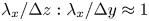 $\lambda _{x}/\Delta z:\lambda _{x}/\Delta y\approx 1$ under near-neutral and unstable conditions. It is found that the aspect ratio
  $\lambda _x/\Delta z$ is greater for the near-neutral case, and becomes progressively smaller as instability increases. Hence similar length (
 $\lambda _x$) structures in unstable conditions will be taller and wider than their near-neutral counterparts. The phase of the cross-spectrum provides a scale-by-scale structure inclination angle. We find that this inclination angle is invariant with scale for the near-neutral case, but with increasing positive buoyancy becomes increasingly scale-dependent. For unstable conditions (e.g.
  $z_s/L = -0.5$), all scales are inclined at steeper angles compared to the near-neutral case, with the smaller scales with
  $\lambda _x/\delta = 1$ exhibiting inclination angles that are approximately twice those of larger scales,
  $\lambda _x/\delta = 6$.
Funding
We acknowledge support from the National Natural Science Foundation of China (no. 92052202) and financial support from the Australian Research Council. Also, X.L. was supported by a CSC scholarship (file no. 201706180037).
Declaration of interests
The authors report no conflict of interest.
Appendix. Outline of a coherent structure
Visualizing the outline of a coherent statistical structure of a streamwise velocity fluctuation in the streamwise/wall-normal plane relies on a simple model based on (3.5) and (3.2). The procedure for plotting a structure such as the example one in figure 10 involves the following steps.
Figure 10. Example of an outline of a coherent streamwise/wall-normal structure of a particular scale and set of ASL parameters (as indicated in the figure).
(i) A wavelength of the structure should be chosen, i.e.
 $\lambda _x = 2\delta$. Note that the structure is visualized in physical space, through the assumption that its streamwise extent equals half the wavelength, $\mathcal {L} \sim \lambda _x/2$.
(ii) A degree of unstable stratification should be chosen, i.e.
$z_s/L = -0.40$ (here $z_s = 2.5$ m).(iii) A reference height, above which the structure is visualized, should be chosen.


A structure outline is then generated through considering a sequence of local heights  $z$. For every height, the angle relative to the fixed reference height is determined from (3.5) and (3.2); this is illustrated by the series of ten grey lines at the left edge of the structure in figure 10. Note that the structure is defined only up to a height that is dictated by the aspect ratio condition, following the trend line in figure 4(b). Thus the wall-normal extent up to which the coherent structure reaches is found by computing
  $\Delta z$ from
  ${A{\kern-4pt}R} _u^{z} \equiv \lambda _x/\Delta z = -1.9\log _{10}(-z_s/L) + 3.5$.


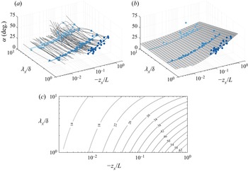


 Open access