


1. Introduction
Cognitively adequate models of language have been a subject of central interest in areas as diverse as philosophy, (computational) linguistics, artificial intelligence, cognitive science, neurology, and intermediate disciplines. Much effort in natural language processing (NLP) has been devoted to obtain representations of linguistic units,Footnote a such as words, that can capture language syntax, semantics,Footnote b and other linguistic aspects for computational processing. One of the primary and successful models for the representation of word semantics are vector space models (VSMs) introduced by Salton, Wong, and Yang (Reference Salton, Wong and Yang1975) and its variations, such as word space models (Schütze Reference Schütze1993), hyperspace analogue to language (Lund and Burgess Reference Lund and Burgess1996), latent semantic analysis (Deerwester et al. Reference Deerwester, Dumais, Furnas, Landauer and Harshman1990), and more recently neural word embeddings, such as word2vec (Mikolov et al. Reference Mikolov, Chen, Corrado and Dean2013a) and neural language models, such as BERT (Devlin et al. Reference Devlin, Chang, Lee and Toutanova2019). In VSMs, a vector representation in a continuous vector space of some fixed dimension is created for each word in the text. VSMs have been empirically justified by results from cognitive science (Gärdenfors Reference Gärdenfors2000).
One influential approach to produce word vector representations in VSMs are distributional representations, which are generally based on the distributional hypothesis first introduced by Harris (Reference Harris1954). The distributional hypothesis presumes that “difference of meaning correlates with difference of distribution” (Harris Reference Harris1954, p. 156). Based on this hypothesis, “words that occur in the same contexts tend to have similar meanings” (Pantel Reference Pantel2005, p. 126), and the meaning of words is defined by contexts in which they (co-)occur. Depending on the specific model employed, these contexts can be either local (the co-occurring words) or global (a sentence or a paragraph or the whole document). In VSMs, models that are obtained based on the distributional hypothesis are called distributional semantic models (DSMs). Word meaning is then modeled as an n-dimensional vector, derived from word co-occurrence counts in a given context. In these models, words with similar distributions tend to have closer representations in the vector space. These approaches to semantics share the usage-based perspective on meaning; that is, representations focus on the meaning of words that comes from their usage in a context. In this way, semantic relationships between words can also be understood using the distributional representations and by measuring the distance between vectors in the vector space (Mitchell and Lapata Reference Mitchell and Lapata2010). Vectors that are close together in this space have similar meanings and vectors that are far away are distant in meaning (Turney and Pantel Reference Turney and Pantel2010). In addition to mere co-occurrence information, some DSMs also take into account the syntactic relationship of word pairs, such as subject–verb relationship, for constructing their vector representations (Padó and Lapata Reference Padó and Lapata2007; Baroni and Lenci Reference Baroni and Lenci2010). Therefore, dependency relations contribute to the construction of the semantic space and capture more linguistic knowledge. These dependency relations are asymmetric and hence reflect the word position and order information in the word vector construction. In these models, text preprocessing is required for building the model, as lexico-syntactic relations have to be extracted first.
Many recent approaches utilize machine learning techniques with the distributional hypothesis to obtain continuous vector representations that reflect the meanings in natural language. One example is word2vec, proposed by Mikolov et al. (Reference Mikolov, Chen, Corrado and Dean2013a, b), which is supposed to capture both syntactic and semantic aspects of words. In general, VSMs have proven to perform well in a number of tasks requiring computation of semantic closeness between words, such as synonymy identification (Landauer and Dumais Reference Landauer and Dumais1997), automatic thesaurus construction (Grefenstette Reference Grefenstette1994), semantic priming and word sense disambiguation (Padó and Lapata Reference Padó and Lapata2007), and many more.
Early VSMs represented each word separately, without considering representations of larger units like phrases or sentences. Consequently, the compositionality properties of language were not considered in VSMs (Mitchell and Lapata Reference Mitchell and Lapata2010). According to Frege’s principle of compositionality (Frege Reference Frege1884), “The meaning of an expression is a function of the meanings of its parts and of the way they are syntactically combined” (Partee Reference Partee2004, p.153). Therefore, the meaning of a complex expression in a natural language is determined by its syntactic structure and the meanings of its constituents (Halvorsen and Ladusaw Reference Halvorsen and Ladusaw1979). On sentence level, the meaning of a sentence such as White mushrooms grow quickly is a function of the meaning of the noun phrase White mushrooms combined as a subject with the meaning of the verb phrase grow quickly. Each phrase is also derived from the combination of its constituents. This way, semantic compositionality allows us to construct long grammatical sentences with complex meanings (Baroni, Bernardi, and Zamparelli Reference Baroni, Bernardi and Zamparelli2014). Approaches have been developed that obtain meaning above the word level and introduce compositionality for DSMs in NLP. These approaches are called compositional distributional semantic models (CDSMs). CDSMs propose word representations and vector space operations (such as vector addition) as the composition operation. Mitchell and Lapata (Reference Mitchell and Lapata2010) propose a framework for vector-based semantic composition in DSMs. They define additive or multiplicative functions for the composition of two vectors and show that compositional approaches generally outperform non-compositional approaches which treat a phrase as the union of single lexical items. Word2vec models also exhibit good compositionality properties using standard vector operations (Mikolov et al. Reference Mikolov, Chen, Corrado and Dean2013a, b). However, these models cannot deal with lexical ambiguity and representations are non-contextualized. Very recently, contextualized (or context-aware) word representation models, such as transformer-based models like BERT (Devlin et al. Reference Devlin, Chang, Lee and Toutanova2019), have been introduced. These models learn to construct distinct representations for different meanings of the words based on their occurrence in different contexts. Moreover, they consider the word order of input text for training the final representations by adding the positional information of words to their representations. These models compute word representations using large neural-based architectures. Moreover, training such models needs rich computational resources. Due to their expensive computational requirements, compressed versions of BERT have been introduced, such as DistilBERT (Sanh et al. Reference Sanh, Debut, Chaumond and Wolf2019). They have shown state-of-the-art performance in downstream NLP tasks, and we refer the reader interested in contextualized word representations to the work by Devlin et al. (Reference Devlin, Chang, Lee and Toutanova2019). Our focus in this article is on light-weight computations of word representations in a given context and the dynamic composition of word representations using algebraic operations.
Despite its simplicity and light-weight computations, one of the downsides of using vector addition (or other commutative operations like the component-wise product) as the compositionality operation is that word order information is inevitably lost. To overcome this limitation while maintaining light-weight computations for compositional representations, this article describes an alternative, word-order-sensitive approach for compositional word representations, called compositional matrix-space models (CMSMs). In such models, word matrices instead of vectors are used as word representations and compositionality is realized via iterated matrix multiplication.
Contributions. The contribution of this work can be grouped into two categories:
-
(1). On the formal, theoretical side, we propose CMSMs as word-level representation models and provide advantageous properties of these models for NLP, showing that they are able to simulate most of the known vector-based compositionality operations and that several CMSMs can be combined into one in a straightforward way. We also investigate expressiveness and computational properties of the languages accepted of a CMSM-based grammar model, called matrix grammars. This contribution is an extended and revised account of results by Rudolph and Giesbrecht (Reference Rudolph and Giesbrecht2010).
-
(2). On the practical side, we provide an exemplary experimental investigation of the practical applicability of CMSMs in English by considering two NLP applications: compositional sentiment analysis and compositionality prediction of short phrases. We chose these two tasks for practical investigations since compositionality properties of the language play an important role in such tasks. For this purpose, we develop two different machine learning techniques for the mentioned tasks and evaluate the performance of the learned model against other distributional compositional models from the literature. By means of these investigations we show that
-
there are scalable methods for learning CMSMs from linguistic corpora and
-
in terms of model quality, the learned models are competitive with other state-of-the-art approaches while requiring significantly fewer parameters.
-
This contribution addresses the question “how to acquire CMSMs automatically in large-scale and for specific purposes” raised by Rudolph and Giesbrecht (Reference Rudolph and Giesbrecht2010). Preliminary results of this contribution concerning the sentiment analysis task have been published by Asaadi and Rudolph (Reference Asaadi and Rudolph2017). In this article, we extend them with hitherto unpublished investigations on compositionality prediction.
Structure. The structure of the article is as follows. We first review compositional distributional models in literature and provide the related work for the task of compositional sentiment analysis and semantic compositionality prediction in Section 2. Then, to introduce CMSMs, we start by providing the necessary basic notions in linear algebra in Section 3. In Section 4, we give a formal account of the concept of compositionality, introduce CMSMs, and argue for the plausibility of CMSMs in the light of structural and functional considerations. Section 5 demonstrates beneficial theoretical properties of CMSMs: we show how common VSM approaches to compositionality can be captured by CMSMs, while they are likewise able to cover symbolic approaches; moreover, we demonstrate how several CMSMs can be combined into one model.
In view of these advantageous properties, CMSMs seem to be a suitable candidate in a diverse range of different tasks of NLP. In Section 6, we focus on ways to elicit information from matrices to leverage CMSMs for NLP tasks like scoring or classification. These established beneficial properties motivate a practical investigation of CMSMs in NLP applications. Therefore, methods for training such models need to be developed, for example, by leveraging appropriate machine learning techniques.
Hence, we address the problem of learning CMSMs in Section 7. Thereby, we focus on a gradient descent method but apply diverse optimizations to increase the method’s efficiency and performance. We propose to apply a two-step learning strategy where the output of the first step serves as the initialization for the second step. The results of the performance evaluation of our learning methods on two tasks are studied in Section 8.2.2. In the first part of the experiments, we investigate our learning method for CMSMs on the task of compositionality prediction of multi-word expressions (MWE). Compositionality prediction is important in downstream NLP tasks such as statistical machine translation (Enache, Listenmaa, and Kolachina Reference Enache, Listenmaa and Kolachina2014; Weller et al. Reference Weller, Cap, Müller, Schulte im Walde and Fraser2014), word-sense disambiguation (McCarthy, Keller, and Carroll Reference McCarthy, Keller and Carroll2003), and text summarization (ShafieiBavani et al. Reference ShafieiBavani, Ebrahimi, Wong and Chen2018) where a method is required to detect whether the words in a phrase are used in a compositional meaning. Therefore, we choose to evaluate the proposed method for CMSMs on the ability to detect the compositionality of phrases. In the second part of the experiments, we evaluate our method on the task of fine-grained sentiment analysis. We choose this task since it allows a direct comparison against two closely related techniques proposed by Yessenalina and Cardie (Reference Yessenalina and Cardie2011) and Irsoy and Cardie (Reference Irsoy and Cardie2015), which also trains a CMSM. We finally conclude by discussing the strengths and limitations of CMSMs in Section 9.
As stated earlier, this article is a consolidated, significantly revised, and considerably extended exposition of work presented in earlier conference and workshop papers (Rudolph and Giesbrecht Reference Rudolph and Giesbrecht2010; Asaadi and Rudolph Reference Asaadi and Rudolph2017).
2. Related work
We were not the first to suggest an extension of classical VSMs to higher-order tensors. Early attempts to apply matrices instead of vectors to text data came from research in information retrieval (Gao, Wang, and Wang Reference Gao, Wang and Wang2004; Liu et al. Reference Liu, Zhang, Yan, Chen, Liu, Bai and Chien2005; Antonellis and Gallopoulos Reference Antonellis and Gallopoulos2006; Cai, He, and Han Reference Cai, He and Han2006). Most proposed models in information retrieval still use a vector-based representation as the basis and then mathematically convert vectors into tensors, without linguistic justification of such a transformation, or they use metadata or ontologies to initialize the models (Sun, Tao, and Faloutsos Reference Sun, Tao and Faloutsos2006; Chew et al. Reference Chew, Bader, Kolda and Abdelali2007; Franz et al. Reference Franz, Schultz, Sizov and Staab2009; Van de Cruys Reference Van de Cruys2010). However, to the best of our knowledge, we were the first to propose an approach of realizing compositionality via consecutive matrix multiplication. In this section, a comprehensive review of related work on existing approaches to modeling words as matrices, distributional semantic compositionality, compositional methods for sentiment analysis, and compositionality prediction of MWEs is provided.
Compositional Distributional Semantic Models. In compositional distributional semantics, different approaches for learning word representations and diverse ways of realizing semantic compositionality are studied. In the following, we discuss the related vector space approaches, which are summarized in Table 1. However, be reminded that our compositional approach will be formulated in matrix space as opposed to vector space.
Table 1. Summary of the literature review in semantic compositionality
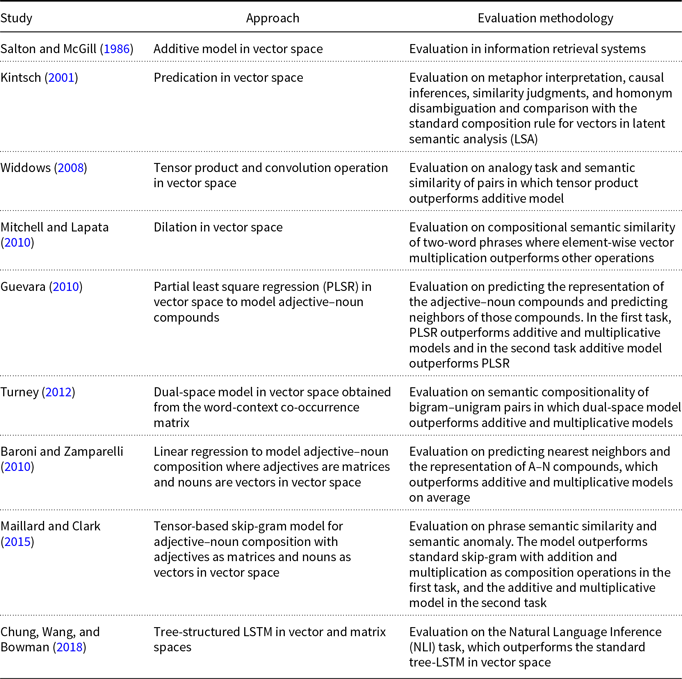
Salton and McGill (Reference Salton and McGill1986) introduce vector addition in VSMs as a composition method, which is the most common method. Given two words
 $w_i$
and
$w_i$
and
 $w_j$
and their associated d-dimensional semantic vector representations
$w_j$
and their associated d-dimensional semantic vector representations
 ${\textbf{u}} \in \mathbb{R}^d$
and
${\textbf{u}} \in \mathbb{R}^d$
and
 ${\textbf{v}} \in \mathbb{R}^d$
, respectively, vector addition is defined as follows:
${\textbf{v}} \in \mathbb{R}^d$
, respectively, vector addition is defined as follows:
 \begin{equation*}\textbf{p} = f({\textbf{v}},{\textbf{u}}) = {\textbf{v}} + {\textbf{u}},\end{equation*}
where
 $\textbf{p} \in \mathbb{R}^d$
is the resulting compositional representation of the phrase
$\textbf{p} \in \mathbb{R}^d$
is the resulting compositional representation of the phrase
 $w_iw_j$
and f is called the composition function. Despite its simplicity, the additive method is not a suitable method of composition because vector addition is commutative. Therefore, it is not sensitive to word order in the sentence, which is a natural property of human language.
$w_iw_j$
and f is called the composition function. Despite its simplicity, the additive method is not a suitable method of composition because vector addition is commutative. Therefore, it is not sensitive to word order in the sentence, which is a natural property of human language.
Among the early attempts to provide more compelling compositional functions in VSMs is the work of Kintsch (Reference Kintsch2001) who is using a more sophisticated composition function to model predicate–argument structures. Kintsch (Reference Kintsch2001) argues that the neighboring words “strengthen features of the predicate that are appropriate for the argument of the predication” (p. 178). For instance, the predicate run depends on the noun as its argument and has a different meaning in, for example, “the horse runs” and “the ship runs before the wind.” Thus, different features are used for composition based on the neighboring words. Also, not all features of a predicate vector are combined with the features of the argument, but only those that are appropriate for the argument.
An alternative seminal work on compositional distributional semantics is by Widdows (Reference Widdows2008). Widdows proposes a number of more advanced vector operations well-known from quantum mechanics for semantic compositionality, such as tensor product and convolution operation to model composition in vector space. Given two vectors
 ${\textbf{u}} \in \mathbb{R}^{d}$
and
${\textbf{u}} \in \mathbb{R}^{d}$
and
 ${\textbf{v}} \in \mathbb{R}^{d}$
, the tensor product of two vectors is a matrix
${\textbf{v}} \in \mathbb{R}^{d}$
, the tensor product of two vectors is a matrix
 $Q \in \mathbb{R}^{d \times d}$
with
$Q \in \mathbb{R}^{d \times d}$
with
 $Q(i,j) = {\textbf{u}}(i){\textbf{v}}(j)$
. Since the number of dimensions increases by tensor product, the convolution operation was introduced to compress the tensor product operation to
$Q(i,j) = {\textbf{u}}(i){\textbf{v}}(j)$
. Since the number of dimensions increases by tensor product, the convolution operation was introduced to compress the tensor product operation to
 $\mathbb{R}^d$
space. Widdows shows the ability of the introduced compositional models to reflect the relational and phrasal meanings on a simplified analogy task and semantic similarity which outperform additive models.
$\mathbb{R}^d$
space. Widdows shows the ability of the introduced compositional models to reflect the relational and phrasal meanings on a simplified analogy task and semantic similarity which outperform additive models.
Mitchell and Lapata (Reference Mitchell and Lapata2010) formulate semantic composition as a function
 $m = f(w_1,w_2,R,K)$
where R is a relation between
$m = f(w_1,w_2,R,K)$
where R is a relation between
 $w_1$
and
$w_1$
and
 $w_2$
and K is additional knowledge. They evaluate the model with a number of addition and multiplication operations for vector combination and introduce dilation as another composition operation. The dilation method decomposes
$w_2$
and K is additional knowledge. They evaluate the model with a number of addition and multiplication operations for vector combination and introduce dilation as another composition operation. The dilation method decomposes
 ${\textbf{v}}$
into a parallel and an orthogonal component to
${\textbf{v}}$
into a parallel and an orthogonal component to
 ${\textbf{u}}$
and then stretches the parallel component to adjust
${\textbf{u}}$
and then stretches the parallel component to adjust
 ${\textbf{v}}$
along
${\textbf{v}}$
along
 ${\textbf{u}}$
:
${\textbf{u}}$
:
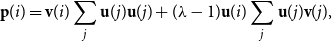 \begin{equation*}{\bf p}(i) = {\textbf{v}}(i) \sum_j {\textbf{u}}(j){\textbf{u}}(j) + (\lambda - 1) {\textbf{u}}(i) \sum_j {\textbf{u}}(j){\textbf{v}}(j),\end{equation*}
where
 $\lambda$
is the dilation factor and p is the composed vector. Therefore,
$\lambda$
is the dilation factor and p is the composed vector. Therefore,
 ${\textbf{u}}$
affects relevant elements of vector
${\textbf{u}}$
affects relevant elements of vector
 ${\textbf{v}}$
in the composition. Evaluation is done on their developed compositional semantic similarity dataset of two-word phrases. They conclude that element-wise vector multiplication outperforms additive models and non-compositional approaches in the semantic similarity of complex expressions.
${\textbf{v}}$
in the composition. Evaluation is done on their developed compositional semantic similarity dataset of two-word phrases. They conclude that element-wise vector multiplication outperforms additive models and non-compositional approaches in the semantic similarity of complex expressions.
Giesbrecht (Reference Giesbrecht2009) evaluates four vector composition operations (addition, element-wise multiplication, tensor product, convolution) in vector space on the task of identifying multi-word units. The evaluation results of the three studies (Widdows Reference Widdows2008; Giesbrecht Reference Giesbrecht2009; Mitchell and Lapata Reference Mitchell and Lapata2010) are not conclusive in terms of which vector operation performs best; the different outcomes might be attributed to the underlying word space models; for example, the models of Widdows (Reference Widdows2008) and Giesbrecht (Reference Giesbrecht2009) feature dimensionality reduction while that of Mitchell and Lapata (Reference Mitchell and Lapata2010) does not.
Guevara (Reference Guevara2010) proposes a linear regression model for adjective–noun (A–N) compositionality. He trains a generic function to compose any adjective and noun vectors and produce the A–N representation. The model which is learned by partial least square regression (PLSR) outperforms additive and multiplicative models in predicting the vector representation of A–Ns. However, the additive model outperforms PLSR in predicting the nearest neighbors in the vector space. As opposed to this work, semantic compositionality in our approach is regardless of the parts of speech (POS), and therefore, the model can be trained to represent different compositional compounds with various POS tags.
Some approaches for obtaining distributional representation of words in VSMs have also been extended to compositional distributional models. Turney (Reference Turney2012) proposes a dual-space model for semantic compositionality. He creates two VSMs from the word-context co-occurrence matrix, one from the noun as the context of the words (called domain space) and the other from the verb as the context of the word (called function space). Therefore, the dual-space model consists of a domain space for determining the similarity in topic or subject, and a function space for computing the similarity in role or relationship. He evaluates the dual-space model on the task of similarity of compositions for pairs of bigram–unigram in which bigram is a noun phrase and unigram is a noun. He shows that the introduced dual-space model outperforms additive and multiplicative models.
Few approaches using matrices for distributional representations of words have been introduced more recently, which are then used for capturing compositionality. A method to drive a distributional representation of A–N phrases is proposed by Baroni and Zamparelli (Reference Baroni and Zamparelli2010) where the adjective serves as a linear function mapping the noun vector to another vector in the same space, which presents the A–N compound. In this method, each adjective has a matrix representation. Using linear regression, they train separate models for each adjective. They evaluate the performance of the proposed approach in predicting the representation of A–N compounds and predicting their nearest neighbors. Results show that their model outperforms additive and multiplicative models on average. A limitation of this model is that a separate model is trained for each adjective, and there is no global training model for adjectives. This is in contrast to our proposed approach in this work.
Maillard and Clark (Reference Maillard and Clark2015) describe a compositional model for learning A–N pairs where, first, word vectors are trained using the skip-gram model with negative sampling (Mikolov et al. Reference Mikolov, Sutskever, Chen, Corrado and Dean2013b). Then, each A–N phrase is considered as a unit, and adjective matrices are trained by optimizing the skip-gram objective function for A–N phrase vectors. The phrase vectors of the objective function are obtained by multiplying the adjective matrix with its noun vector. Noun vectors in this step are fixed. Results on the phrase semantic similarity task show that the model outperforms the standard skip-gram with addition and multiplication as the composition operations. Moreover, the model outperforms additive and multiplicative models in the semantic anomaly task.
More recently, Chung et al. (Reference Chung, Wang and Bowman2018) introduced a learning method for a matrix-based compositionality model using a deep learning architecture. They propose a tree-structured long short-term memory (LSTM) approach for the task of natural language inference (NLI) to learn the word matrices. In their method, the model learns to transform the pre-trained input word embeddings (e.g., word2vec) to word matrix embeddings (lift layer). Then word matrices are composed hierarchically using matrix multiplication to obtain the representation of sentences (composition layer). The sentence representations are then used to train a classifier for the NLI task.
Semantic Compositionality Evaluation. Table 2 summarizes the literature on techniques to evaluate the existing compositional models on capturing semantic compositionality.
Table 2. Summary of the literature review in compositionality prediction
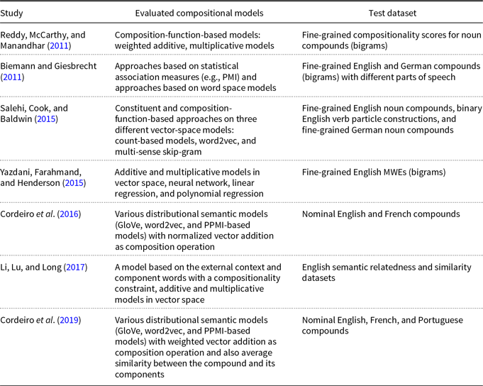
Reddy et al. (Reference Reddy, McCarthy and Manandhar2011) study the performance of compositional distributional models on compositionality prediction of multi-word compounds. For this purpose, they provide a dataset of noun compounds with fine-grained compositionality scores as well as literality scores for constituent words based on human judgments. They analyze both constituent-based models and composition-function-based models regarding compositionality prediction of the proposed compounds. In constituent-based models, they study the relations between the contribution of constituent words and the judgments on compound compositionality. They argue if a word is used literally in a compound, most probably it shares a common co-occurrence with the corresponding compound. Therefore, they evaluate different composition functions applied on constituent words and compute their similarity with the literality scores of phrases. In composition-function-based models, they evaluate weighted additive and multiplicative composition functions on their dataset and investigate the similarity between the composed word vector representations and the compound vector representation. Results show that in both models, additive composition outperforms other functions.
Biemann and Giesbrecht (Reference Biemann and Giesbrecht2011) aim at extracting non-compositional phrases using automatic distributional models that assign a compositionality score to a phrase. This score denotes the extent to which the compositionality assumption holds for a given expression. For this purpose, they created a dataset of English and German phrases which attracted several models ranging from statistical association measures and word space models submitted in a shared task of SemEval’11.
Salehi et al. (Reference Salehi, Cook and Baldwin2015) explore compositionality prediction of MWEs using constituent-based and composition-function-based approaches on three different VSMs, consisting of count-based models, word2vec, and multi-sense skip-gram model. In constituent-based models, they study the relation between the contribution of constituent words and the judgments on compound compositionality. In the composition-function-based models, they study the additive model in vector space on compositionality.
Yazdani et al. (Reference Yazdani, Farahmand and Henderson2015) then explore different compositional models ranging from simple to complex models such as neural networks (NNs) for non-compositionality prediction of a dataset of MWEs. The dataset is created by Farahmand, Smith, and Nivre (Reference Farahmand, Smith and Nivre2015), which consists of MWEs annotated with non-compositionality judgments. Representation of words is obtained from word2vec of Mikolov et al. (Reference Mikolov, Chen, Corrado and Dean2013a) and the models are trained using compounds extracted from a Wikipedia dump corpus, assuming that most compounds are compositional. Therefore, the trained models are expected to give a relatively high error to non-compositional compounds. They improve the accuracy of the models using latent compositionality annotation and show that this method improves the performance of nonlinear models significantly. Their results show that polynomial regression model with quadratic degree outperforms other models.
Cordeiro et al. (Reference Cordeiro, Ramisch, Idiart and Villavicencio2016) and their extended work (Cordeiro et al. Reference Cordeiro, Villavicencio, Idiart and Ramisch2019) are closely related to our work regarding the compositionality prediction task. They explore the performance of unsupervised vector addition and multiplication over various DSMs (GloVe, word2vec, and PPMI-based models) regarding predicting semantic compositionality of noun compounds over previously proposed English and French datasets in Cordeiro et al. (Reference Cordeiro, Ramisch, Idiart and Villavicencio2016) and a combination of previously and newly proposed English, French, and Portuguese datasets in Cordeiro et al. (Reference Cordeiro, Villavicencio, Idiart and Ramisch2019). Normalized vector addition in Cordeiro et al. (Reference Cordeiro, Ramisch, Idiart and Villavicencio2016) is considered as the composition function, and the performance of word embeddings is investigated using different setting of parameters for training them.
Cordeiro et al. (Reference Cordeiro, Villavicencio, Idiart and Ramisch2019) consider a weighted additive model as the composition function in which the weights of head and modifier words in the compounds range from 0 to 1, meaning that the similarity between head only word and the compound, the similarity between modifier only word and the compound, as well as the similarity between equally weighted head and modifier words and the compound are evaluated. Moreover, they consider the average of the similarity between head-compound pair and modifier-compound pair and compute the correlation between the average similarity score and the human judgments on the compositionality of compound. In both works, they also study the impact of corpus preprocessing on capturing compositionality with DSMs. Furthermore, the influence of different settings of DSMs parameters and corpus size for training is studied. In our work, we evaluate our proposed compositional model using their introduced English dataset. We compare the performance of our model with the weighted additive model as well as other unsupervised and supervised models and provide a more comprehensive collection of compositional models for evaluation. In the weighted additive model, we report the best model obtained by varying the weights of the head and modifier words of the compound.
In a work by Li et al. (Reference Li, Lu and Long2017), a hybrid method to learn the representation of MWEs from their external context and constituent words with a compositionality constraint is proposed. The main idea is to learn MWE representations based on a weighted linear combination of both external context and component words, where the weight is based on the compositionality of the MWEs. Evaluations are done on the task of semantic similarity and semantic relatedness between bigrams and unigrams. Recent deep learning techniques also focus on modeling the compositionality of more complex texts without considering the compositionality of the smaller parts such as Wu and Chi (Reference Wu and Chi2017), which is out of the scope of our study. None of the mentioned works, however, have investigated the performance of CMSMs in compositionality prediction of short phrases on MWE datasets.
Compositional Sentiment Analysis. There is a lot of research interest in the task of sentiment analysis in NLP. The task is to classify the polarity of a text (negative, positive, neutral) or assign a real-valued score, showing the polarity and intensity of the text. In the following, we review the literature, which is summarized in Table 3.
Table 3. Summary of the literature review in compositional sentiment analysis. SST denotes Stanford Sentiment Treebank dataset
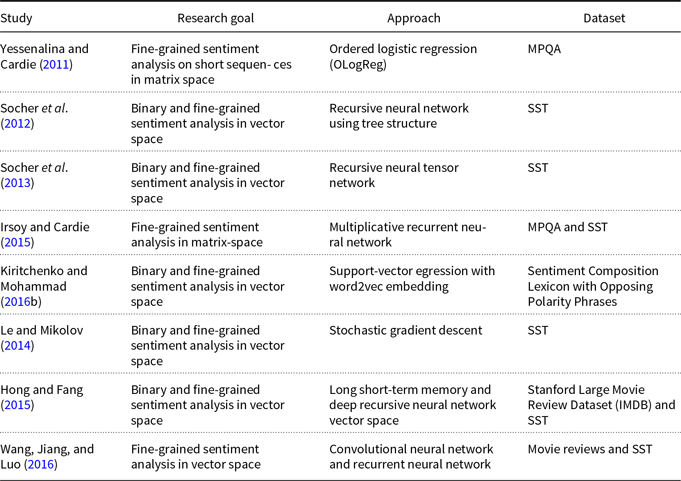
Yessenalina and Cardie (Reference Yessenalina and Cardie2011) propose the first supervised learning technique for CMSMs in fine-grained sentiment analysis on short sequences after it was introduced by Rudolph and Giesbrecht (Reference Rudolph and Giesbrecht2010). This work is closely related to ours as we propose learning techniques for CMSMs in the task of fine-grained sentiment analysis. Yessenalina and Cardie (Reference Yessenalina and Cardie2011) apply ordered logistic regression (OLogReg) with constraints on CMSMs to acquire a matrix representation of words. The learning parameters in their method include the word matrices as well as a set of thresholds (also called constraints), which indicate the intervals for sentiment classes since they convert the sentiment classes to ordinal labels. They argue that the learning problem for CMSMs is not a convex problem, so it must be trained carefully and specific attention has to be devoted to a good initialization, to avoid getting stuck in local optima. Therefore, they propose a model for ordinal scale sentiment prediction and address the optimization problem using OLogReg with constraints on sentiment intervals to relax the non-convexity. Finally, the trained model assigns real-valued sentiment scores to phrases. We address this issue in our proposed learning method for CMSMs. As opposed to Yessenalina and Cardie (Reference Yessenalina and Cardie2011)’s work, we address a sentiment regression problem directly and our learning method does not need to constrain the sentiment scores to the certain intervals. Therefore, the number of parameters to learn is reduced to only word matrices.
Recent approaches have focused on learning different types of NNs for sentiment analysis, such as the work of Socher et al. (Reference Socher, Huval, Manning and Ng2012) and (2013). Moreover, the superiority of multiplicative composition has been confirmed in their studies. Socher et al. (Reference Socher, Huval, Manning and Ng2012) propose a recursive NN which learns the vector representations of phrases in a tree structure. Each word and phrase is represented by a vector
 ${\textbf{v}}$
and a matrix M. When two constituents in the tree are composed, the matrix of one is multiplied with the vector of the other constituent. Therefore, the composition function is parameterized by the words that participate in it. Socher et al. (Reference Socher, Huval, Manning and Ng2012) predict the binary (only positive and negative) sentiment classes and fine-grained sentiment scores using the trained recursive NN on their developed Stanford Sentiment Treebank dataset. This means that new datasets must be preprocessed to generate the parse trees for evaluating the proposed method. A problem with this method is that the number of parameters becomes very large as it needs to store a matrix and a vector for each word and phrase in the tree together with the fully labeled parse tree. In contrast, our CMSM does not rely on parse trees, and therefore, preprocessing of the dataset is not required. Each word is represented only with matrices where the compositional function is the standard matrix multiplication, which replaces the recursive computations with a sequential computation.
${\textbf{v}}$
and a matrix M. When two constituents in the tree are composed, the matrix of one is multiplied with the vector of the other constituent. Therefore, the composition function is parameterized by the words that participate in it. Socher et al. (Reference Socher, Huval, Manning and Ng2012) predict the binary (only positive and negative) sentiment classes and fine-grained sentiment scores using the trained recursive NN on their developed Stanford Sentiment Treebank dataset. This means that new datasets must be preprocessed to generate the parse trees for evaluating the proposed method. A problem with this method is that the number of parameters becomes very large as it needs to store a matrix and a vector for each word and phrase in the tree together with the fully labeled parse tree. In contrast, our CMSM does not rely on parse trees, and therefore, preprocessing of the dataset is not required. Each word is represented only with matrices where the compositional function is the standard matrix multiplication, which replaces the recursive computations with a sequential computation.
Socher et al. (Reference Socher, Perelygin, Wu, Chuang, Manning, Ng and Potts2013) address the issue of the high number of parameters in the work by Socher et al. (Reference Socher, Huval, Manning and Ng2012) by introducing a recursive neural tensor network in which a global tensor-based composition function is defined. In this model, a tensor layer is added to their standard recursive NN where the vectors of two constituents are multiplied with a shared third-order tensor in this layer and then passed to the standard layer. The output is a composed vector of words which is then composed with the next word in the same way. The model is evaluated on both fine-grained and binary (only positive and negative) sentiment classification of phrases and sentences. Similar to Socher et al. (Reference Socher, Huval, Manning and Ng2012), a fully labeled parse tree is needed. In contrast, our model in this work does not rely on parse trees.
Irsoy and Cardie (Reference Irsoy and Cardie2015) propose a multiplicative recurrent NN (mRNN) for fine-grained sentiment analysis inspired from CMSMs (Rudolph and Giesbrecht Reference Rudolph and Giesbrecht2010). They show that their proposed architecture is more generic than CMSM and outperforms additive NNs in sentiment analysis. In their architecture, a shared third-order tensor is multiplied with each word vector input to obtain the word matrix in CMSMs. They use pre-trained word vectors of dimension 300 from word2vec (Mikolov et al. Reference Mikolov, Sutskever, Chen, Corrado and Dean2013b) and explore different sizes of matrices extracted from the shared third-order tensor. The results on the task of sentiment analysis are compared to the work by Yessenalina and Cardie (Reference Yessenalina and Cardie2011). We also compare the results of our model training on the same task to this approach since it is closely related to our work. However, in our approach, we do not use word vectors as input. Instead, the input word matrices are trained directly without using a shared tensor. We show that our model performs better while using fewer dimensions.
Kiritchenko and Mohammad (Reference Kiritchenko and Mohammad2016a) create a dataset of unigrams, bigrams, and trigrams, which contains specific phrases with at least one negative and one positive word. For instance, a phrase “happy tears” contains a positive-carrying sentiment word (happy) and a negative word (tears). They analyze the performance of support-vector regression (SVR) with different features on the developed dataset. We show that our approach can predict the sentiment score of such phrases in matrix space with a much lower number of features than SVR.
There are a number of deep NN models on the task of sentiment compositional analysis such as Hong and Fang (Reference Hong and Fang2015) who apply LSTM and deep recursive-NNs, and Wang et al. (Reference Wang, Jiang and Luo2016) who combine convolutional NNs and recurrent NNs leading to a significant improvement in sentiment analysis of short text. Le and Mikolov (Reference Le and Mikolov2014) also propose paragraph vector to represent long texts such as sentences and paragraphs, which is applied in the task of binary and fine-grained sentiment analysis. The model consists of a vector for each paragraph as well as the word vectors, which are concatenated to predict the next word in the context. Vectors are trained using stochastic gradient descent method. These techniques do not focus on training word representations that can be readily composed and therefore are not comparable directly to our proposed model.
3. Preliminaries
In this section, we recap some aspects of linear algebra to the extent needed for our considerations about CMSMs. For a more thorough treatise, we refer the reader to a linear algebra textbook (such as Strang Reference Strang1993).
Vectors. Given a natural number n, an n-dimensional vector
 ${\textbf{v}}$
over the reals can be seen as a list (or tuple) containing n real numbers
${\textbf{v}}$
over the reals can be seen as a list (or tuple) containing n real numbers
 $r_1,\ldots,r_n \in \mathbb{R}$
, written
$r_1,\ldots,r_n \in \mathbb{R}$
, written
 ${\textbf{v}} = (r_1\quad r_2\quad \cdots\quad r_n)$
. Vectors will be denoted by lowercase bold font letters and we will use the notation
${\textbf{v}} = (r_1\quad r_2\quad \cdots\quad r_n)$
. Vectors will be denoted by lowercase bold font letters and we will use the notation
 ${\textbf{v}}(i)$
to refer to the ith entry of vector
${\textbf{v}}(i)$
to refer to the ith entry of vector
 ${\textbf{v}}$
. As usual, we write
${\textbf{v}}$
. As usual, we write
 $\mathbb{R}^n$
to denote the set of all n-dimensional vectors with real-valued entries. Vectors can be added entry-wise, that is,
$\mathbb{R}^n$
to denote the set of all n-dimensional vectors with real-valued entries. Vectors can be added entry-wise, that is,
 $(r_1\quad \cdots\quad r_n) + (r^{\prime}_1\quad \cdots\quad r^{\prime}_n) = (r_1\!+\!r^{\prime}_1\quad \cdots\quad r_n\!+\!r^{\prime}_n)$
. Likewise, the entry-wise product (also known as Hadamard product) is defined by
$(r_1\quad \cdots\quad r_n) + (r^{\prime}_1\quad \cdots\quad r^{\prime}_n) = (r_1\!+\!r^{\prime}_1\quad \cdots\quad r_n\!+\!r^{\prime}_n)$
. Likewise, the entry-wise product (also known as Hadamard product) is defined by
 $(r_1\ \ \cdots\ \ r_n)\ \odot\ (r^{\prime}_1\ \ \cdots\ \ r^{\prime}_n) = (r_1\cdot r^{\prime}_1\ \ \cdots\ \ r_n\cdot r^{\prime}_n)$
.
$(r_1\ \ \cdots\ \ r_n)\ \odot\ (r^{\prime}_1\ \ \cdots\ \ r^{\prime}_n) = (r_1\cdot r^{\prime}_1\ \ \cdots\ \ r_n\cdot r^{\prime}_n)$
.
Matrices. Given two natural numbers n and m, an
 $n\times m$
matrix over the reals is an array of real numbers with n rows and m columns. We will use capital letters to denote matrices and, given a matrix M we will write M(i,j) to refer to the entry in the ith row and the jth column:
$n\times m$
matrix over the reals is an array of real numbers with n rows and m columns. We will use capital letters to denote matrices and, given a matrix M we will write M(i,j) to refer to the entry in the ith row and the jth column:
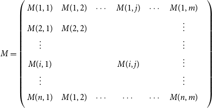 \begin{equation*} \mbox{$M =$} \left(\begin{array}{@{\ }c@{\quad}c@{\quad}c@{\quad}c@{\quad}c@{\quad}c@{\quad}} M(1,1) & M(1,2) & \cdots & M(1,j) & \cdots & M(1,m) \\[4pt] M(2,1) & M(2,2) & & & & \vdots \\[1pt] \vdots & & & & & \vdots \\[1pt] M(i,1) & & & M(i,j) & & \vdots \\[1pt] \vdots & & & & & \vdots \\[1pt] M(n,1) & M(1,2) & \cdots & \cdots & \cdots & M(n,m) \\[4pt] \end{array}\right) \end{equation*}
The set of all
 $n\times m$
matrices with real number entries is denoted by
$n\times m$
matrices with real number entries is denoted by
 $\mathbb{R}^{n\times m}$
. Obviously, m-dimensional vectors can be seen as
$\mathbb{R}^{n\times m}$
. Obviously, m-dimensional vectors can be seen as
 $1 \times m$
matrices. A matrix can be transposed by exchanging columns and rows: given the
$1 \times m$
matrices. A matrix can be transposed by exchanging columns and rows: given the
 $n\times m$
matrix M, its transposed version
$n\times m$
matrix M, its transposed version
 $M^T$
is an
$M^T$
is an
 $m\times n$
matrix defined by
$m\times n$
matrix defined by
 $M^T(i,j) = M(j,i)$
.
$M^T(i,j) = M(j,i)$
.
Third-order Tensors. A third-order tensor of dimension
 $d \times n \times m$
over real values is a d-array of
$d \times n \times m$
over real values is a d-array of
 $n \times m$
matrices. Third-order tensors are denoted by uppercase bold font letters, and
$n \times m$
matrices. Third-order tensors are denoted by uppercase bold font letters, and
 ${\bf T}(i,j,k)$
refers to row j and column k of matrix i in T.
${\bf T}(i,j,k)$
refers to row j and column k of matrix i in T.
 $\mathbb{R}^{d \times n \times m}$
indicates the set of all tensors with real number elements.
$\mathbb{R}^{d \times n \times m}$
indicates the set of all tensors with real number elements.
Linear Mappings. Beyond being merely array-like data structures, matrices correspond to a certain type of functions, so-called linear mappings, having vectors as input and output. More precisely, an
 $n\times m$
matrix M applied to an m-dimensional vector
$n\times m$
matrix M applied to an m-dimensional vector
 ${\textbf{v}}$
yields an n-dimensional vector
${\textbf{v}}$
yields an n-dimensional vector
 ${\textbf{v}}'$
(written:
${\textbf{v}}'$
(written:
 ${\textbf{v}} M = {\textbf{v}}'$
) according to
${\textbf{v}} M = {\textbf{v}}'$
) according to
 \begin{equation*}{\textbf{v}}'(i) = \sum_{j=1}^m {\textbf{v}}(j)\cdot M(i,j).\end{equation*}
Linear mappings can be concatenated, giving rise to the notion of standard matrix multiplication: we write
 $M_1 M_2$
to denote the matrix that corresponds to the linear mapping defined by applying first
$M_1 M_2$
to denote the matrix that corresponds to the linear mapping defined by applying first
 $M_1$
and then
$M_1$
and then
 $M_2$
. Formally, the matrix product of the
$M_2$
. Formally, the matrix product of the
 $n\times \ell$
matrix
$n\times \ell$
matrix
 $M_1$
and the
$M_1$
and the
 $\ell \times m$
matrix
$\ell \times m$
matrix
 $M_2$
is an
$M_2$
is an
 $n\times m$
matrix
$n\times m$
matrix
 $M = M_1 M_2$
defined by
$M = M_1 M_2$
defined by
 \begin{equation*}M(i,j) = \sum_{k=1}^\ell M_1(i,k)\cdot M_2(k,j).\end{equation*}
Note that the matrix product is associative (i.e.,
 $(M_1M_2)M_3 = M_1(M_2M_3)$
always holds, thus parentheses can be omitted) but not commutative (
$(M_1M_2)M_3 = M_1(M_2M_3)$
always holds, thus parentheses can be omitted) but not commutative (
 $M_1M_2 = M_2M_1$
does not hold in general, that is, the order of the multiplied matrices matters).
$M_1M_2 = M_2M_1$
does not hold in general, that is, the order of the multiplied matrices matters).
Permutations. Given a natural number n, a permutation on
 $\{1\ldots n\}$
is a bijection (i.e., a mapping that is one-to-one and onto)
$\{1\ldots n\}$
is a bijection (i.e., a mapping that is one-to-one and onto)
 $\Phi{\,:\,}\{1\ldots n\} \to \{1\ldots n\}$
. A permutation can be seen as a “reordering scheme” on a list with n elements: the element at position i will get the new position
$\Phi{\,:\,}\{1\ldots n\} \to \{1\ldots n\}$
. A permutation can be seen as a “reordering scheme” on a list with n elements: the element at position i will get the new position
 $\Phi(i)$
in the reordered list. Likewise, a permutation can be applied to a vector resulting in a rearrangement of the entries. We write
$\Phi(i)$
in the reordered list. Likewise, a permutation can be applied to a vector resulting in a rearrangement of the entries. We write
 $\Phi^n$
to denote the permutation corresponding to the n-fold application of
$\Phi^n$
to denote the permutation corresponding to the n-fold application of
 $\Phi$
and
$\Phi$
and
 $\Phi^{-1}$
to denote the permutation that “undoes”
$\Phi^{-1}$
to denote the permutation that “undoes”
 $\Phi$
.
$\Phi$
.
Given a permutation
 $\Phi$
, the corresponding permutation matrix
$\Phi$
, the corresponding permutation matrix
 $M_\Phi$
is defined by
$M_\Phi$
is defined by
 \begin{equation*}M_\Phi(i,j) = \left\{\begin{array}{l}1 \mbox{ if }\Phi(j)=i,\\0 \mbox{ otherwise.}\\\end{array}\right.\end{equation*}
Then, obviously permuting a vector according to
 $\Phi$
can be expressed in terms of matrix multiplication as well, since we obtain, for any vector
$\Phi$
can be expressed in terms of matrix multiplication as well, since we obtain, for any vector
 ${\textbf{v}}\in\mathbb{R}^n$
,
${\textbf{v}}\in\mathbb{R}^n$
,
 \begin{equation*}\Phi({\textbf{v}}) = {\textbf{v}} M_\Phi.\end{equation*}
Likewise, iterated application (
 $\Phi^n$
) and the inverses
$\Phi^n$
) and the inverses
 $\Phi^{-n}$
carry over naturally to the corresponding notions in matrices.
$\Phi^{-n}$
carry over naturally to the corresponding notions in matrices.
4. A matrix-based model of compositionality
Frege’s principle of compositionality states that “the meaning of an expression is a function of the meanings of its parts and of the way they are syntactically combined” (Partee Reference Partee2004, p. 153). Also, according to Partee, ter Meulen, and Wall (Reference Partee, ter Meulen and Wall1993, p. 334) the mathematical formulation of the compositionality principle involves “representing both the syntax and the semantics as algebras and the semantic interpretation as a homomorphic mapping from the syntactic algebra into the semantic algebra.”
The underlying principle of compositional semantics is that the meaning of a composed sequence can be derived from the meaning of its constituent tokensFootnote
c
by applying a composition operation. More formally, the underlying idea can be described mathematically as follows: given a mapping
 $\mbox{$[\,\!\![$}{\,\cdot\,}\mbox{$]\,\!\!]$}: \Sigma \to \mathbb{S}$
from a set of tokens (words)
$\mbox{$[\,\!\![$}{\,\cdot\,}\mbox{$]\,\!\!]$}: \Sigma \to \mathbb{S}$
from a set of tokens (words)
 $\Sigma$
into some semantic space
$\Sigma$
into some semantic space
 $\mathbb{S}$
(the elements of which we will simply call “meanings”), we find a semantic composition operation
$\mathbb{S}$
(the elements of which we will simply call “meanings”), we find a semantic composition operation
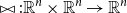
 $\bowtie: \mathbb{S}^* \to \mathbb{S}$
mapping sequences of meanings to meanings such that the meaning of a sequence of tokens
$\bowtie: \mathbb{S}^* \to \mathbb{S}$
mapping sequences of meanings to meanings such that the meaning of a sequence of tokens
 $s=\sigma_1\sigma_2\ldots\sigma_k$
can be obtained by applying
$s=\sigma_1\sigma_2\ldots\sigma_k$
can be obtained by applying
 $\bowtie$
to the sequence
$\bowtie$
to the sequence
 $\mbox{$[\,\!\![$}{\sigma_1}\mbox{$]\,\!\!]$}\mbox{$[\,\!\![$}{\sigma_2}\mbox{$]\,\!\!]$}\ldots\mbox{$[\,\!\![$}{\sigma_k}\mbox{$]\,\!\!]$}$
. This situation, displayed in Figure 1, qualifies
$\mbox{$[\,\!\![$}{\sigma_1}\mbox{$]\,\!\!]$}\mbox{$[\,\!\![$}{\sigma_2}\mbox{$]\,\!\!]$}\ldots\mbox{$[\,\!\![$}{\sigma_k}\mbox{$]\,\!\!]$}$
. This situation, displayed in Figure 1, qualifies
 $\mbox{$[\,\!\![$}{\cdot}\mbox{$]\,\!\!]$}$
as a homomorphism between
$\mbox{$[\,\!\![$}{\cdot}\mbox{$]\,\!\!]$}$
as a homomorphism between
 $(\Sigma^*,\cdot)$
and
$(\Sigma^*,\cdot)$
and
 $(\mathbb{S},\bowtie)$
.
$(\mathbb{S},\bowtie)$
.
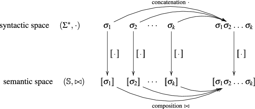
Figure 1. Semantic mapping as homomorphism.
A great variety of linguistic models are subsumed by this general idea ranging from purely symbolic approaches (like type systems and categorial grammars) to statistical models (like vector space and word space models). At the first glance, the underlying encodings of word semantics as well as the composition operations differ significantly. However, we argue that a great variety of them can be incorporated – and even freely inter-combined – into a unified model where the semantics of simple tokens and complex phrases is expressed by matrices and the composition operation is standard matrix multiplication that considers the position of tokens in the sequence.
More precisely, in CMSMs, we have
 $\mathbb{S} = \mathbb{R}^{m\times m}$
, that is, the semantic space consists of quadratic matrices, and the composition operator
$\mathbb{S} = \mathbb{R}^{m\times m}$
, that is, the semantic space consists of quadratic matrices, and the composition operator
 $\bowtie$
coincides with matrix multiplication as introduced in Section 3.
$\bowtie$
coincides with matrix multiplication as introduced in Section 3.
We next provide an argument in favor of CMSMs due to their “algebraic plausibility.” Most linear-algebra-based operations that have been proposed to model composition in language models (such as vector addition or the Hadamard product) are both associative and commutative. Thereby, they realize a multiset (or bag-of-words) semantics which makes them oblivious of structural differences of phrases conveyed through word order. For instance, in an associative and commutative model, the statements “Oswald killed Kennedy” and “Kennedy killed Oswald” would be mapped to the same semantic representation. For this reason, having commutativity “built-in” in language models seems a very arguable design decision.
On the other hand, language is inherently stream-like and sequential; thus, associativity alone seems much more justifiable. Ambiguities which might be attributed to non-associativity (such as the different meanings of the sentence “The man saw the girl with the telescope.”) can be resolved easily by contextual cues.
As mentioned before, matrix multiplication is associative but non-commutative, whence we propose it as more adequate for modeling compositional semantics of language.
5. The power of CMSMs
In the following, we argue that CMSMs have diverse desirable properties from a theoretical perspective, justifying our confidence that they can serve as a generic approach to modeling compositionality in natural language.
5.1 CMSMs capture compositional VSMs
In VSMs, numerous vector operations have been used to model composition (Widdows Reference Widdows2008). We show how common composition operators can be simulated by CMSMs.Footnote
d
For each such vector composition operation
 $\bowtie: \mathbb{R}^n \times \mathbb{R}^n \to \mathbb{R}^n$
, we will provide a pair of functions
$\bowtie: \mathbb{R}^n \times \mathbb{R}^n \to \mathbb{R}^n$
, we will provide a pair of functions
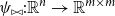 $\psi_{\bowtie}: \mathbb{R}^n \to \mathbb{R}^{m\times m}$
and
$\psi_{\bowtie}: \mathbb{R}^n \to \mathbb{R}^{m\times m}$
and
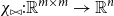 $\chi_{\bowtie}: \mathbb{R}^{m\times m} \to \mathbb{R}^n$
satisfying
$\chi_{\bowtie}: \mathbb{R}^{m\times m} \to \mathbb{R}^n$
satisfying
 $\chi_{\bowtie}(\psi_{\bowtie}({\textbf{v}})))={\textbf{v}}$
for all
$\chi_{\bowtie}(\psi_{\bowtie}({\textbf{v}})))={\textbf{v}}$
for all
 ${\textbf{v}} \in \mathbb{R}^n$
. These functions translate between the vector representation and the matrix representation in a way such that for all
${\textbf{v}} \in \mathbb{R}^n$
. These functions translate between the vector representation and the matrix representation in a way such that for all
 ${\textbf{v}}_1, \ldots, {\textbf{v}}_k \in \mathbb{R}^n$
holds
${\textbf{v}}_1, \ldots, {\textbf{v}}_k \in \mathbb{R}^n$
holds
 \begin{equation*}{\textbf{v}}_1 \bowtie \ldots \bowtie {\textbf{v}}_k = \chi_{\bowtie}(\psi_{\bowtie}({\textbf{v}}_1) \ldots \psi_{\bowtie}({\textbf{v}}_k)),\end{equation*}
where
 $\psi_{\bowtie}({\textbf{v}}_i)\psi_{\bowtie}({\textbf{v}}_j)$
denotes matrix multiplication of the matrices assigned to
$\psi_{\bowtie}({\textbf{v}}_i)\psi_{\bowtie}({\textbf{v}}_j)$
denotes matrix multiplication of the matrices assigned to
 ${\textbf{v}}_i$
and
${\textbf{v}}_i$
and
 ${\textbf{v}}_j$
. This allows us to simulate a
${\textbf{v}}_j$
. This allows us to simulate a
 $\bowtie$
-compositional VSM by a matrix-space model where matrix multiplication is the composition operation (see Figure 2). We can in fact show that vector addition, element-wise vector multiplication, holographic reduced representation, and permutation based composition approaches are captured by CMSMs. See Appendix A for detailed discussion and proofs.
$\bowtie$
-compositional VSM by a matrix-space model where matrix multiplication is the composition operation (see Figure 2). We can in fact show that vector addition, element-wise vector multiplication, holographic reduced representation, and permutation based composition approaches are captured by CMSMs. See Appendix A for detailed discussion and proofs.
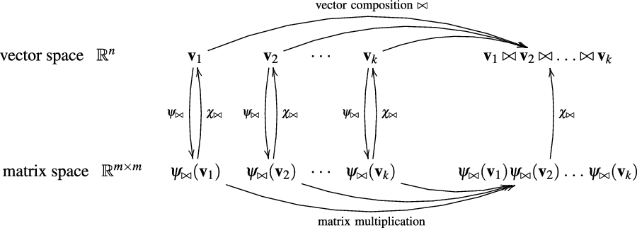
Figure 2. Simulating compositional VSM via CMSMs.
5.2 CMSMs capture symbolic approaches
Now we will elaborate on symbolic approaches to language, that is, discrete grammar formalisms, and show how they can conveniently be embedded into CMSMs. This might come as a surprise, as the apparent likeness of CMSMs to VSMs may suggest incompatibility to discrete settings.
Group Theory. Group theory and grammar formalisms based on groups and pre-groups play an important role in computational linguistics (Lambek Reference Lambek1958; Dymetman Reference Dymetman1998). From the perspective of our compositionality framework, those approaches employ a group (or pre-group)
 $(G,\cdot)$
as the semantic space
$(G,\cdot)$
as the semantic space
 $\mathbb{S}$
where the group operation (often written as multiplication) is used as composition operation
$\mathbb{S}$
where the group operation (often written as multiplication) is used as composition operation
 $\bowtie$
.
$\bowtie$
.
According to Cayley’s theorem (Cayley Reference Cayley1854), every group G is isomorphic to a permutation group on some set S. Hence, assuming finiteness of G and consequently S, we can encode group-based grammar formalisms into CMSMs in a straightforward way using permutation matrices of size
 $|S|\times|S|$
.
$|S|\times|S|$
.
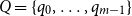
Regular Languages. Regular languages constitute a basic type of languages characterized by a symbolic formalism. We will show how to select the assignment
 $\mbox{$[\,\!\![$}{\,\cdot\,}\mbox{$]\,\!\!]$}$
for a CMSM such that the matrix associated with a token sequence exhibits whether this sequence belongs to a given regular language, that is, if it is accepted by a given finite state automaton. As usual, we define a nondeterministic finite automaton
$\mbox{$[\,\!\![$}{\,\cdot\,}\mbox{$]\,\!\!]$}$
for a CMSM such that the matrix associated with a token sequence exhibits whether this sequence belongs to a given regular language, that is, if it is accepted by a given finite state automaton. As usual, we define a nondeterministic finite automaton
 $\mathcal{A}=(Q,\Sigma,\Delta,Q_\textrm{I},Q_\textrm{F})$
with
$\mathcal{A}=(Q,\Sigma,\Delta,Q_\textrm{I},Q_\textrm{F})$
with
 $Q=\{q_0,\ldots,q_{m-1}\}$
being the set of states,
$Q=\{q_0,\ldots,q_{m-1}\}$
being the set of states,
 $\Sigma$
the input alphabet,
$\Sigma$
the input alphabet,
 $\Delta \subseteq Q \times \Sigma \times Q$
the transition relation, and
$\Delta \subseteq Q \times \Sigma \times Q$
the transition relation, and
 $Q_\textrm{I}$
and
$Q_\textrm{I}$
and
 $Q_\textrm{F}$
being the sets of initial and final states, respectively.
$Q_\textrm{F}$
being the sets of initial and final states, respectively.
Then we assign to every token
 $\sigma \in \Sigma$
the
$\sigma \in \Sigma$
the
 $m\times m$
matrix
$m\times m$
matrix
 $\mbox{$[\,\!\![$}{\sigma}\mbox{$]\,\!\!]$}=M$
with
$\mbox{$[\,\!\![$}{\sigma}\mbox{$]\,\!\!]$}=M$
with
 \begin{equation*}M(i,j) = \left\{\begin{array}{l}1 \mbox{ if }(q_i,\sigma,q_j)\in\Delta,\\0 \mbox{ otherwise.}\\\end{array}\right.\end{equation*}
Hence essentially, the matrix M encodes all state transitions which can be caused by the input
 $\sigma$
. Likewise, for a sequence
$\sigma$
. Likewise, for a sequence
 $s=\sigma_1\ldots\sigma_k\in \Sigma^*$
, the matrix
$s=\sigma_1\ldots\sigma_k\in \Sigma^*$
, the matrix
 $M_s := \mbox{$[\,\!\![$}{\sigma_1}\mbox{$]\,\!\!]$}\ldots \mbox{$[\,\!\![$}{\sigma_k}\mbox{$]\,\!\!]$}$
will encode all state transitions mediated by s.
$M_s := \mbox{$[\,\!\![$}{\sigma_1}\mbox{$]\,\!\!]$}\ldots \mbox{$[\,\!\![$}{\sigma_k}\mbox{$]\,\!\!]$}$
will encode all state transitions mediated by s.
5.3 Intercombining CMSMs
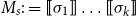
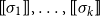
Another central advantage of the proposed matrix-based models for word meaning is that several matrix models can be easily combined into one. Again assume a sequence
 $s=\sigma_1\ldots\sigma_k$
of tokens with associated matrices
$s=\sigma_1\ldots\sigma_k$
of tokens with associated matrices
 $\mbox{$[\,\!\![$}{\sigma_1}\mbox{$]\,\!\!]$}, \ldots, \mbox{$[\,\!\![$}{\sigma_k}\mbox{$]\,\!\!]$}$
according to one specific model and matrices
$\mbox{$[\,\!\![$}{\sigma_1}\mbox{$]\,\!\!]$}, \ldots, \mbox{$[\,\!\![$}{\sigma_k}\mbox{$]\,\!\!]$}$
according to one specific model and matrices
 $\mbox{$(\,\!\![$}{\sigma_1}\mbox{$]\,\!\!)$}, \ldots, \mbox{$(\,\!\![$}{\sigma_k}\mbox{$]\,\!\!)$}$
according to another.
$\mbox{$(\,\!\![$}{\sigma_1}\mbox{$]\,\!\!)$}, \ldots, \mbox{$(\,\!\![$}{\sigma_k}\mbox{$]\,\!\!)$}$
according to another.
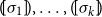
Then we can combine the two models into one
 $\mbox{$\{\,\!\![$}{\ \cdot\ }\mbox{$]\,\!\!\}$}$
by assigning to
$\mbox{$\{\,\!\![$}{\ \cdot\ }\mbox{$]\,\!\!\}$}$
by assigning to
 $\sigma_i$
the matrix
$\sigma_i$
the matrix
 \begin{equation*}\mbox{$\{\,\!\![$}{\sigma_i}\mbox{$]\,\!\!\}$} =\left(\begin{array}{ccc@{\ \ }|cccc}& & & & 0 & \cdots & 0 \\& \mbox{$[\,\!\![$}{\sigma_i}\mbox{$]\,\!\!]$} & & & \vdots & \ddots & \\& & & & 0 & & 0 \\\hline0 & \cdots & 0 & & & & \\\vdots & \ddots & & & & \mbox{$(\,\!\![$}{\sigma_i}\mbox{$]\,\!\!)$} & \\0 & & 0 & & & & \\\end{array}\right)\! .\end{equation*}
By doing so, we obtain the correspondence
 \begin{equation*}\mbox{$\{\,\!\![$}{\sigma_1}\mbox{$]\,\!\!\}$}\ldots\mbox{$\{\,\!\![$}{\sigma_k}\mbox{$]\,\!\!\}$} =\left(\begin{array}{c@{\ }c@{\ }cc|cc@{\ }c@{\ }c}& & & & & 0 & \cdots & 0 \\& \mbox{$[\,\!\![$}{\sigma_1}\mbox{$]\,\!\!]$}\ldots\mbox{$[\,\!\![$}{\sigma_k}\mbox{$]\,\!\!]$} & & & & \vdots & \ddots & \\& & & & & 0 & & 0 \\\hline0 & \cdots & 0 & & & & & \\\vdots & \ddots & & & & & \mbox{$(\,\!\![$}{\sigma_1}\mbox{$]\,\!\!)$}\ldots\mbox{$(\,\!\![$}{\sigma_k}\mbox{$]\,\!\!)$} & \\0 & & 0 & & & & & \\\end{array}\right)\! .\end{equation*}
In other words, the semantic compositions belonging to two CMSMs can be executed “in parallel.” Mark that by providing non-zero entries for the upper right and lower left matrix part, information exchange between the two models can be easily realized.
6. Eliciting linguistic information from matrix representations
In the previous sections, we have argued in favor of using quadratic matrices as representatives for the meaning of words and – by means of composition – phrases. The matrix representation of a phrase thus obtained then arguably carries semantic information encoded in a certain way. This necessitates a “decoding step” where the information of interest is elicited from the matrix representation and is represented in different forms.
In the following, we will discuss various possible ways of eliciting the linguistic information from the matrix representation of phrases. Thereby we distinguish if this information is in the form of a vector, a scalar, or a boolean value. Proofs for the given theorems and propositions can be found in Appendix B.
6.1 Vectors
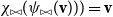
Vectors can represent various syntactic and semantic information of words and phrases and are widely used in many NLP tasks. The information in matrix representations in CMSMs can be elicited in a vector shape allowing for their comparison and integration with other NLP vector-space approaches. There are numerous options for a vector extraction function
 $\chi: \mathbb{R}^{m\times m} \to \mathbb{R}^n$
, among them the different functions
$\chi: \mathbb{R}^{m\times m} \to \mathbb{R}^n$
, among them the different functions
 $\chi_{\bowtie}$
, introduced in Section 5.1.
$\chi_{\bowtie}$
, introduced in Section 5.1.
One alternative option can be derived from an idea already touched in the second part of Section 5.2, according to which CMSMs can be conceived as state transition systems, where states are represented by vectors, and multiplying a state-vector with a matrix implements a transition from the corresponding state to another. We will provide a speculative neuropsychological underpinning of this idea in Section 9. If we assume that processing an input sequence will always start from a fixed initial state
 $\alpha \in {R}^{m}$
, then the state after processing
$\alpha \in {R}^{m}$
, then the state after processing
 $s = \sigma_1\ldots \sigma_k$
will be
$s = \sigma_1\ldots \sigma_k$
will be
 $\alpha M_{\sigma_1}\ldots M_{\sigma_k} = \alpha M_{s}$
. Consequently, one simple but plausible vector extraction operation would be given by the function
$\alpha M_{\sigma_1}\ldots M_{\sigma_k} = \alpha M_{s}$
. Consequently, one simple but plausible vector extraction operation would be given by the function
 $\chi_\alpha$
where the vector v associated with a matrix M is
$\chi_\alpha$
where the vector v associated with a matrix M is
 \begin{equation*}v = \chi_\alpha(M) = \alpha M.\end{equation*}
6.2 Scalars
Scalars (i.e., real values) may also represent semantic information in NLP tasks, such as semantic similarity degree in similarity tasks or sentiment score in sentiment analysis. Also, the information in scalar form requires less storage than matrices or vectors. To map a matrix
 $M \in \mathbb{R}^{m\times m}$
to a scalar value, we may employ any
$M \in \mathbb{R}^{m\times m}$
to a scalar value, we may employ any
 $m^2$
-ary function which takes as input all entries of M and delivers a scalar value. There are plenty of options for such a function. In this article, we will be focusing on the class of functions brought about by two mapping vectors from
$m^2$
-ary function which takes as input all entries of M and delivers a scalar value. There are plenty of options for such a function. In this article, we will be focusing on the class of functions brought about by two mapping vectors from
 $\mathbb{R}^m$
, called
$\mathbb{R}^m$
, called
 $\alpha$
and
$\alpha$
and
 $\beta$
, mapping a matrix M to the scalar value r via
$\beta$
, mapping a matrix M to the scalar value r via
 \begin{equation*}r = \alpha M \beta^\top.\end{equation*}
Again, we can motivate this choice along the lines of transitional plausibility. If, as argued in the previous section,
 $\alpha$
represents an “initial mental state,” then, for a sequence s, the vector
$\alpha$
represents an “initial mental state,” then, for a sequence s, the vector
 $v_s = \alpha M_s \in \mathbb{R}^m$
represents the mental state after receiving the sequence s. Then
$v_s = \alpha M_s \in \mathbb{R}^m$
represents the mental state after receiving the sequence s. Then
 $r_s = \alpha M_s \beta^\top = v_s\beta^\top$
is the scalar obtained from a linear combination of the entries of
$r_s = \alpha M_s \beta^\top = v_s\beta^\top$
is the scalar obtained from a linear combination of the entries of
 $v_s$
, that is,
$v_s$
, that is,
 $r_s=b_1\cdot v(1) + \ldots + b_m\cdot v(m)$
, where
$r_s=b_1\cdot v(1) + \ldots + b_m\cdot v(m)$
, where
 $\beta = (b_1 \quad \cdots \quad b_m)$
.
$\beta = (b_1 \quad \cdots \quad b_m)$
.
Clearly, choosing appropriate “mapping vectors”
 $\alpha$
and
$\alpha$
and
 $\beta$
will dependent on the NLP task and the problem to be solved. However, it turns out that with a proper choice of the token-to-matrix mapping, we can restrict
$\beta$
will dependent on the NLP task and the problem to be solved. However, it turns out that with a proper choice of the token-to-matrix mapping, we can restrict
 $\alpha$
and
$\alpha$
and
 $\beta$
to a very specific form.
$\beta$
to a very specific form.
To this end, let
 \begin{equation*}\alpha = e_1 =\left(1 \quad0 \quad\cdots \quad0\right)\mbox{ and }\beta = e_m =\left(0 \quad\cdots \quad0 \quad1\right),\end{equation*}
which only moderately restricts the expressivity of our model as made formally precise in the following theorem.
Theorem 1 Given matrices
 $M_1,\ldots,M_\ell \in \mathbb{R}^{m\times m}$
and vectors
$M_1,\ldots,M_\ell \in \mathbb{R}^{m\times m}$
and vectors
 $\alpha,\beta \in \mathbb{R}^{m}$
, there are matrices
$\alpha,\beta \in \mathbb{R}^{m}$
, there are matrices
 $\hat{M}_1,\ldots,\hat{M}_\ell \in \mathbb{R}^{(m+1)\times (m+1)}$
such that for every sequence
$\hat{M}_1,\ldots,\hat{M}_\ell \in \mathbb{R}^{(m+1)\times (m+1)}$
such that for every sequence
 $i_1\cdots i_k$
of numbers from
$i_1\cdots i_k$
of numbers from
 $\{1,\ldots,\ell\}$
holds
$\{1,\ldots,\ell\}$
holds
 \begin{equation*} \alpha M_{i_1}\cdots M_{i_k} \beta^\top = e_1 \hat{M}_{i_1}\cdots\hat{M}_{i_k} e_{m+1}^\top . \end{equation*}
In words, this theorem guarantees that for every CMSM-based scoring model with arbitrary vectors
 $\alpha$
and
$\alpha$
and
 $\beta$
there is another such model (with dimensionality increased by one), where
$\beta$
there is another such model (with dimensionality increased by one), where
 $\alpha$
and
$\alpha$
and
 $\beta$
are distinct unit vectors. This theorem justifies our choice mentioned above.
$\beta$
are distinct unit vectors. This theorem justifies our choice mentioned above.
6.3 Boolean values
Boolean values can be also obtained from matrix representations. Obviously, any function
 $\zeta: \mathbb{R}^{m\times m} \to \{\textrm{true},\textrm{false}\}$
can be seen as a binary classifier which accepts or rejects a sequence of tokens as being part of the formal language
$\zeta: \mathbb{R}^{m\times m} \to \{\textrm{true},\textrm{false}\}$
can be seen as a binary classifier which accepts or rejects a sequence of tokens as being part of the formal language
 $L_\zeta$
defined by
$L_\zeta$
defined by
 \begin{equation*}L = \{ \sigma_1\ldots\sigma_k \mid \zeta([\!\!\,[{\sigma_1}]\,\!\!] \ldots [\!\!\,[{\sigma_k}]\,\!\!]) = \textrm{true}\}.\end{equation*}
One option for defining such a function
 $\zeta$
is to first obtain a scalar (for instance using the mapping discussed before), as described in the preceding section and then compare that scalar against a given threshold value.Footnote
e
Of course, one can also perform several such comparisons. This idea gives rise to the notion of matrix grammars.
$\zeta$
is to first obtain a scalar (for instance using the mapping discussed before), as described in the preceding section and then compare that scalar against a given threshold value.Footnote
e
Of course, one can also perform several such comparisons. This idea gives rise to the notion of matrix grammars.
Definition 1 (Matrix Grammars). Let
 $\Sigma$
be an alphabet. A matrix grammar
$\Sigma$
be an alphabet. A matrix grammar
 $\mathcal{M}$
of degree m is defined as the pair
$\mathcal{M}$
of degree m is defined as the pair
 $\langle\ [\!\!\,[ \cdot ]\,\!\!],\ AC\rangle$
where
$\langle\ [\!\!\,[ \cdot ]\,\!\!],\ AC\rangle$
where
 $[\!\!\,[ \cdot ]\,\!\!]$
is a mapping from
$[\!\!\,[ \cdot ]\,\!\!]$
is a mapping from
 $\Sigma$
to
$\Sigma$
to
 $m\times m$
matrices and
$m\times m$
matrices and
 $AC = \{\langle\alpha_1,\beta_1,r_1\rangle, \ldots, \langle\alpha_\ell,\beta_\ell,r_\ell\rangle\}$
with
$AC = \{\langle\alpha_1,\beta_1,r_1\rangle, \ldots, \langle\alpha_\ell,\beta_\ell,r_\ell\rangle\}$
with
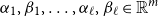 $\alpha_1,\beta_1,\ldots,\alpha_\ell,\beta_\ell \in \mathbb{R}^m$
and
$\alpha_1,\beta_1,\ldots,\alpha_\ell,\beta_\ell \in \mathbb{R}^m$
and
 $r_1,\ldots,r_\ell\in \mathbb{R}$
is a finite set of acceptance conditions. The language generated by
$r_1,\ldots,r_\ell\in \mathbb{R}$
is a finite set of acceptance conditions. The language generated by
 $\mathcal{M}$
(denoted by
$\mathcal{M}$
(denoted by
 $L(\mathcal{M})$
) contains a token sequence
$L(\mathcal{M})$
) contains a token sequence
 $\sigma_1\ldots\sigma_k\in\Sigma^*$
exactly if
$\sigma_1\ldots\sigma_k\in\Sigma^*$
exactly if
 $\alpha_i [\!\!\,[ \sigma_1 ]\,\!\!] \ldots [\!\!\,[ \sigma_k ]\,\!\!] \beta^T_i \geq r_i$
for all
$\alpha_i [\!\!\,[ \sigma_1 ]\,\!\!] \ldots [\!\!\,[ \sigma_k ]\,\!\!] \beta^T_i \geq r_i$
for all
 $i\in\{1,\ldots, \ell\}$
. We will call a language L matricible if
$i\in\{1,\ldots, \ell\}$
. We will call a language L matricible if
 $L=L(\mathcal{M})$
for some matrix grammar
$L=L(\mathcal{M})$
for some matrix grammar
 $\mathcal{M}$
.
$\mathcal{M}$
.
Then, the following proposition is a direct consequence from the preceding section.
Proposition 1 Regular languages are matricible.
However, as demonstrated by the subsequent examples, many non-regular and even non-context-free languages are also matricible, hinting at the expressivity of matrix grammars.
Example 1 Define
 $\mathcal{M}\langle\ \mbox{$[\,\!\![$}{\,\cdot\,}\mbox{$]\,\!\!]$},\ AC\rangle$
with
$\mathcal{M}\langle\ \mbox{$[\,\!\![$}{\,\cdot\,}\mbox{$]\,\!\!]$},\ AC\rangle$
with
 $\Sigma = \{a, b, c\}$
as well as
$\Sigma = \{a, b, c\}$
as well as
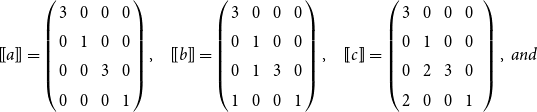 \begin{equation*} \begin{array}[t]{l@{\quad}l@{\quad}l} \mbox{$[\,\!\![$}{a}\mbox{$]\,\!\!]$} = \left(\begin{array}{llll} 3 \ \ & 0 \ \ & 0 \ \ & 0 \\ 0 & 1 & 0 & 0 \\ 0 & 0 & 3 & 0 \\ 0 & 0 & 0 & 1 \\ \end{array}\right), & \mbox{$[\,\!\![$}{b}\mbox{$]\,\!\!]$} = \left(\begin{array}{llll} 3 \ \ & 0 \ \ & 0 \ \ & 0 \\ 0 & 1 & 0 & 0 \\ 0 & 1 & 3 & 0 \\ 1 & 0 & 0 & 1 \\ \end{array}\right), & \mbox{$[\,\!\![$}{c}\mbox{$]\,\!\!]$} = \left(\begin{array}{llll} 3 \ \ & 0 \ \ & 0 \ \ & 0 \ \ \\ 0 & 1 & 0 & 0 \\ 0 & 2 & 3 & 0 \\ 2 & 0 & 0 & 1 \\ \end{array}\right),\ { and}\\ \end{array} \end{equation*}
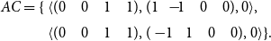 \begin{equation*} \begin{array}{r@{\ }l} AC=\{ & \langle(0\quad 0 \quad 1 \quad 1),(1\quad\ \!\!\!\!-\!\!1\quad 0 \quad 0),0 \rangle, \\ & \langle(0\quad 0 \quad 1 \quad 1),(-\!1\quad\! 1\quad 0 \quad 0),0 \rangle\}. \end{array} \end{equation*}
Then
 $L(\mathcal{M})$
contains exactly all palindromes from
$L(\mathcal{M})$
contains exactly all palindromes from
 $\{a,b,c\}^*$
, that is, the words
$\{a,b,c\}^*$
, that is, the words
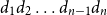 $d_1 d_2 \ldots d_{n-1} d_n$
for which
$d_1 d_2 \ldots d_{n-1} d_n$
for which
 $d_1 d_2 \ldots d_{n-1} d_n = d_n d_{n-1} \ldots d_2 d_1$
.
$d_1 d_2 \ldots d_{n-1} d_n = d_n d_{n-1} \ldots d_2 d_1$
.
Example 2 Define
 $\mathcal{M}=\langle\ \mbox{$[\,\!\![$}{\,\cdot\,}\mbox{$]\,\!\!]$},\ AC\rangle$
with
$\mathcal{M}=\langle\ \mbox{$[\,\!\![$}{\,\cdot\,}\mbox{$]\,\!\!]$},\ AC\rangle$
with
 $\Sigma = \{a, b, c\}$
as well as
$\Sigma = \{a, b, c\}$
as well as
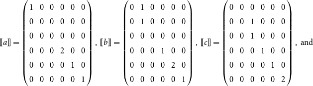 \begin{equation*} \begin{array}[t]{lll} \mbox{$[\,\!\![$}{a}\mbox{$]\,\!\!]$} = \left( \begin{array}{llllll} 1 \ \ & 0 \ \ & 0 \ \ & 0 \ \ & 0 \ \ & 0 \\ 0 & 0 & 0 & 0 & 0 & 0 \\ 0 & 0 & 0 & 0 & 0 & 0 \\ 0 & 0 & 0 & 2 & 0 & 0 \\ 0 & 0 & 0 & 0 & 1 & 0 \\ 0 & 0 & 0 & 0 & 0 & 1 \\ \end{array}\right), & \mbox{$[\,\!\![$}{b}\mbox{$]\,\!\!]$} = \left( \begin{array}{llllll} 0 \ \ & 1 \ \ & 0 \ \ & 0 \ \ & 0 \ \ & 0 \\ 0 & 1 & 0 & 0 & 0 & 0 \\ 0 & 0 & 0 & 0 & 0 & 0 \\ 0 & 0 & 0 & 1 & 0 & 0 \\ 0 & 0 & 0 & 0 & 2 & 0 \\ 0 & 0 & 0 & 0 & 0 & 1 \\ \end{array}\right), & \mbox{$[\,\!\![$}{c}\mbox{$]\,\!\!]$} = \left( \begin{array}{llllll} 0 \ \ & 0 \ \ & 0 \ \ & 0 \ \ & 0 \ \ & 0 \\ 0 & 0 & 1 & 0 & 0 & 0 \\ 0 & 0 & 1 & 0 & 0 & 0 \\ 0 & 0 & 0 & 1 & 0 & 0 \\ 0 & 0 & 0 & 0 & 1 & 0 \\ 0 & 0 & 0 & 0 & 0 & 2 \\ \end{array}\right), \mbox{ and} \end{array} \end{equation*}
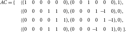 \begin{equation*} \begin{array}{r@{\quad}l} \mbox{ $AC=\{$} & \langle(1\quad 0 \quad 0 \quad 0\quad 0\quad 0),(0\quad 0 \quad 1 \quad 0\quad 0\quad 0),1 \rangle, \\ & \langle(0\quad 0 \quad 0 \quad 1\quad 1\quad 0),(0\quad 0\quad 0 \quad 1\quad \!\!\!\!-\!\!1 \quad 0),0 \rangle, \\ & \langle(0\quad 0 \quad 0 \quad 0\quad 1\quad 1),(0\quad 0\quad 0 \quad 0\quad 1\quad \!\!\!\!-\!\!1),0 \rangle, \\ & \langle(0\quad 0 \quad 0 \quad 1\quad 1\quad 0),(0\quad 0\quad 0 \quad \!\!\!\!-\!\!1 \quad 0\quad 1),0 \rangle\mbox{ $\}.$} \end{array} \end{equation*}
Then
 $L(\mathcal{M})$
is the (non-context-free) language
$L(\mathcal{M})$
is the (non-context-free) language
 $\{a^mb^mc^m \mid m>0\}$
.
$\{a^mb^mc^m \mid m>0\}$
.
The following properties of matrix grammars and matricible language are straightforward.
Proposition 2 All languages characterized by a set of linear equations on the letter counts are matricible.
Proposition 3 The intersection of two matricible languages is again a matricible language.
Note that the fact that the language
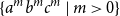 $\{a^mb^mc^m \mid m>0\}$
is matricible, as demonstrated in Example 2, is a straightforward consequence of the Propositions 1, 2, and 3, since the language in question can be described as the intersection of the regular language
$\{a^mb^mc^m \mid m>0\}$
is matricible, as demonstrated in Example 2, is a straightforward consequence of the Propositions 1, 2, and 3, since the language in question can be described as the intersection of the regular language
 $a^+b^+c^+$
with the language characterized by the equations
$a^+b^+c^+$
with the language characterized by the equations
 $x_a-x_b=0$
and
$x_a-x_b=0$
and
 $x_b-x_c=0$
. We proceed by giving another account of the expressivity of matrix grammars by showing undecidability of the emptiness problem.
$x_b-x_c=0$
. We proceed by giving another account of the expressivity of matrix grammars by showing undecidability of the emptiness problem.
Proposition 4 The problem whether there is a word which is accepted by a given matrix grammar is undecidable.
These results demonstrate that matrix grammars cover a wide range of formal languages. Nevertheless some important questions remain open and need to be clarified next:
-
Are all context-free languages matricible? We conjecture that this is not the case.Footnote f Note that this question is directly related to the question whether Lambek calculus can be modeled by matrix grammars.
-
Are matricible languages closed under concatenation? That is: given two arbitrary matricible languages
 $L_1,L_2$
, is the language
$L=\{w_1w_2 \mid w_1\in L_1, w_2\in L_2\}$
again matricible? Being a property common to all language types from the Chomsky hierarchy, answering this question is surprisingly non-trivial for matrix grammars.
$L_1,L_2$
, is the language
$L=\{w_1w_2 \mid w_1\in L_1, w_2\in L_2\}$
again matricible? Being a property common to all language types from the Chomsky hierarchy, answering this question is surprisingly non-trivial for matrix grammars.


In case of a negative answer to one of the above questions it might be worthwhile to introduce an extended notion of context grammars to accommodate those desirable properties. For example, allowing for some nondeterminism by associating several matrices to one token would ensure closure under concatenation.
7. On learning of CMSMs
In the previous sections, we have shown many advantageous theoretical properties of CMSMs, demonstrating their principled suitability and expressivity in compositional NLP tasks.
However, for practical applicability, methods are needed to automatically acquire the word-to-matrix assignments from available data. This important aspect – learning of CMSMs – has remained largely unexplored with few notable exceptions (Yessenalina and Cardie Reference Yessenalina and Cardie2011; Giesbrecht Reference Giesbrecht2014). Methods for training such models can be inspired by appropriate machine learning methods. Training CMSMs is supposed to yield a type of word embedding, assigning to each word a preferably low-dimensional real-valued matrix. Thereby, similar to word vectors, each word matrix is supposed to contain syntactic and semantic information about the word. In the following, we describe options for supervised learning of CMSMs.
As discussed by Asaadi and Rudolph (Reference Asaadi and Rudolph2016), there is a close relationship between CMSMs and weighted finite automata (WFA, cf. Sakarovitch Reference Sakarovitch2009), so the problem of learning CMSMs could be mapped to the problem of learning WFA to extract the matrix representation of words. In fact, several methods for learning WFAs have been described (Balle, Hamilton, and Pineau Reference Balle, Hamilton and Pineau2014; Balle and Mohri Reference Balle and Mohri2015), for example based on the principles of expectation maximization (Dempster, Laird, and Rubin Reference Dempster, Laird and Rubin1977) and method of moments (Pearson Reference Pearson1894). However, in the context of the NLP tasks investigated by us, these techniques performed very poorly in terms of scalability and accuracy; hence, we reverted to gradient descent-based methods.
Gradient descent is an iterative optimization algorithm which is applied to linear and nonlinear problems. In gradient descent, the goal is to find the local minimum/maximum of an objective function by taking steps proportional to the negative/positive gradient of the function at the current point toward the local optimum. In many problems, gradient descent is used to minimize the cost function or the error function by estimating the parameter values of the model.
There are several variants of gradient descent optimization methods. One basic distinction made is that of batch versus stochastic learning. Given a set of training examples, in batch gradient descent, parameter updates are done at each iteration to minimize the sum of the error functions of all training examples, while in stochastic gradient descent parameters are updated after seeing a training example. We found stochastic gradient descent to be a suitable optimization method for learning CMSMs. The specific learning task is to train the model by adapting the word matrix representations iteratively to locally minimize the cost function. Each word matrix is updated according to the gradient descent update principle until finally, the trained word matrices in the CMSM represent (good approximations of) the syntactic and semantics of compositional texts.
In the following, we will describe three variants of CMSM learning methods for two different scenarios: First, in Section 7.1, we will look into learning techniques for compositional phrase scoring models, that is, tasks where phrases are assigned a “score,” being a scalar value. Two variants of CMSM learning, that is, plain gradient descent and gradual gradient descent, are designed for this purpose and will be investigated in the sentiment analysis task. Second, in Section 7.2, we address the scenario aimed at simulating a compositional vector embedding for phrases by means of a CMSM, for which we also present a gradient descent learning method. This approach will be investigated for the compositionality prediction task.
7.1 Gradient descent for phrase scoring
We start by describing the supervised learning task for phrase scoring. We assume to be given a training set containing pairs
 $(s_i,\omega_i)$
of phrases
$(s_i,\omega_i)$
of phrases
 $s_i$
and real values
$s_i$
and real values
 $\omega_i$
(representing
$\omega_i$
(representing
 $s_i$
’s associated score) for
$s_i$
’s associated score) for
 $i \in \{1,\ldots,N\}$
with N the size of training set, in which
$i \in \{1,\ldots,N\}$
with N the size of training set, in which
 $s_i=\sigma_1 \ldots \sigma_{k_i}$
is a phrase consisting of
$s_i=\sigma_1 \ldots \sigma_{k_i}$
is a phrase consisting of
 $k_i$
tokens (words) and
$k_i$
tokens (words) and
 $\omega_i$
is a scalar value as the score of the corresponding sequence (phrase)
$\omega_i$
is a scalar value as the score of the corresponding sequence (phrase)
 $s_i$
. Recall that a CMSM assigns to each word
$s_i$
. Recall that a CMSM assigns to each word
 $\sigma_j$
a matrix
$\sigma_j$
a matrix
 $M_{\sigma_j} \in \mathbb{R}^{m\times m}$
. Then the matrix representation of some phrase
$M_{\sigma_j} \in \mathbb{R}^{m\times m}$
. Then the matrix representation of some phrase
 $s=\sigma_1 \ldots \sigma_{k}$
is the matrix product of the word matrices in the corresponding order:
$s=\sigma_1 \ldots \sigma_{k}$
is the matrix product of the word matrices in the corresponding order:
 \begin{equation*}M_s =M_{\sigma_1}M_{\sigma_2}\ldots M_{\sigma_k}=[\!\!\,[\sigma_1]\,\!\!][\!\!\,[\sigma_2]\,\!\!]\ldots[\!\!\,[\sigma_k]\,\!\!].\end{equation*}
To finally associate a scalar value
 $\omega_s$
to a phrase s, we map the matrix representation of s to a real number using the mapping vectors
$\omega_s$
to a phrase s, we map the matrix representation of s to a real number using the mapping vectors
 ${\textbf{e}}_1,{\textbf{e}}_m \in \mathbb{R}^m$
as follows:
${\textbf{e}}_1,{\textbf{e}}_m \in \mathbb{R}^m$
as follows:
 \begin{equation*}\omega_s = {\textbf{e}}_1 M_{s} {\textbf{e}}_m^\top.\end{equation*}
7.1.1 Plain gradient descent
We first take all the words in the training set as our vocabulary, creating for each a quadratic matrix of size
 $m\times m$
. This provides us with the initial word-to-matrix mapping
$m\times m$
. This provides us with the initial word-to-matrix mapping
 $[\!\!\,[\cdot]\,\!\!]$
. For every phrase
$[\!\!\,[\cdot]\,\!\!]$
. For every phrase
 $s_i = \sigma_1\ldots \sigma_{k_i}$
from the training set, we compute its predicted score
$s_i = \sigma_1\ldots \sigma_{k_i}$
from the training set, we compute its predicted score
 $\hat{\omega_i}$
as given above, that is, via
$\hat{\omega_i}$
as given above, that is, via
 \begin{equation*}\hat{\omega_i} = {\textbf{e}}_1 M_{s_i} {\textbf{e}}_m^\top = {\textbf{e}}_1 [\!\!\,[\sigma_1]\,\!\!][\!\!\,[\sigma_2]\,\!\!]\ldots[\!\!\,[\sigma_{k_i}]\,\!\!] {\textbf{e}}_m^\top.\end{equation*}
Then, we apply the batch gradient descent optimization method on the training set to minimize the error function defined as the sum of the squared error (SSE)
 \begin{equation*}E([\!\!\,[\cdot]\,\!\!]) = \frac{1}{2} \sum_{i=1}^{N}(\hat{\omega_i} - \omega_i)^2,\end{equation*}
where
 $\hat{\omega_i}$
is the predicted score,
$\hat{\omega_i}$
is the predicted score,
 $\omega_i$
is the target score from the training set to be learned, and N is the size of the training set. To prevent from over-fitting and ill-conditioned matrices in learning, we let
$\omega_i$
is the target score from the training set to be learned, and N is the size of the training set. To prevent from over-fitting and ill-conditioned matrices in learning, we let
 \begin{equation*} C([\!\!\,[\cdot]\,\!\!]) = E([\!\!\,[\cdot]\,\!\!]) + \textit{penalty}([\!\!\,[\cdot]\,\!\!]), \end{equation*}
adding a penalty term to the optimization problem. In this work, we consider L2 regularization, that is, we let
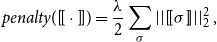 \begin{equation*} \textit{penalty}([\!\!\,[\cdot]\,\!\!]) = \frac{\lambda}{2}\sum_{\sigma}\left|\left|[\!\!\,[\sigma]\,\!\!]\right|\right|^2_2, \end{equation*}
where
 $\lambda$
is the regularization parameter. In batch gradient descent, at each iteration, parameter values are updated to converge to the local optimum. In this work, the parameters to be updated are the word matrices. Therefore, we update each word matrix
$\lambda$
is the regularization parameter. In batch gradient descent, at each iteration, parameter values are updated to converge to the local optimum. In this work, the parameters to be updated are the word matrices. Therefore, we update each word matrix
 $M_{\sigma}$
according to
$M_{\sigma}$
according to
 \begin{equation*} M^{\prime}_{\sigma} = M_{\sigma} - \eta \cdot (\frac{\partial C([\!\!\,[\cdot]\,\!\!])}{\partial M_{\sigma}}) = M_{\sigma} - \eta \cdot (\frac{\partial E([\!\!\,[\cdot]\,\!\!])}{\partial M_{\sigma}} + \lambda M_{\sigma}), \end{equation*}
where
 $\eta$
is the step size toward the local minimum of the error function, called learning rate. L2 regularization is used because it is differentiable with respect to weight matrices.
$\eta$
is the step size toward the local minimum of the error function, called learning rate. L2 regularization is used because it is differentiable with respect to weight matrices.
Following Petersen and Pedersen (Reference Petersen and Pedersen2012), the derivative of the predicted score
 $\hat{\omega_i}$
for a phrase
$\hat{\omega_i}$
for a phrase
 $s_i=\sigma_1 \ldots \sigma_{k_i}$
with respect to the j-th word-matrix
$s_i=\sigma_1 \ldots \sigma_{k_i}$
with respect to the j-th word-matrix
 $M_{\sigma_j} = [\!\!\,[\sigma_j]\,\!\!]$
is computed by
$M_{\sigma_j} = [\!\!\,[\sigma_j]\,\!\!]$
is computed by
 \begin{equation*}\frac{\partial \hat{\omega_i}}{\partial M_{\sigma_j}} = \frac{\partial (\alpha M_{\sigma_1} \cdots M_{\sigma_j} \cdots M_{\sigma_{k_i}} \beta^\top)}{\partial M_{\sigma_j}} = (\alpha M_{\sigma_1} \cdots M_{\sigma_{j-1}} )^\top (M_{\sigma_{j+1}} \cdots M_{\sigma_k} \beta^\top)^\top.\end{equation*}
If a word
 ${x_j}$
occurs several times in the phrase, then the partial derivative of the phrase with respect to
${x_j}$
occurs several times in the phrase, then the partial derivative of the phrase with respect to
 $M_{\sigma_j}$
is the sum of partial derivatives with respect to each occurrence of
$M_{\sigma_j}$
is the sum of partial derivatives with respect to each occurrence of
 $M_{\sigma_j}$
.
$M_{\sigma_j}$
.
7.1.2 Gradual gradient descent
In gradual gradient descent optimization, we (1) perform an “informed initialization” exploiting available scoring information for one-word phrases (unigrams), (2) apply a first learning step only on parts of the matrices and using scored one- and two-word phrases from our training set (unigrams and bigrams), and (3) use the matrices obtained in this step as initialization for training the full matrices on the full training set.
Initialization. In this step, we first take all the words in the training data as our vocabulary, creating quadratic matrices of size
 $m\times m$
with entries from a normal distribution
$m\times m$
with entries from a normal distribution
 $\mathcal{N}(\mu,\sigma^2)$
. Then, we consider the words which appear in unigram phrases
$\mathcal{N}(\mu,\sigma^2)$
. Then, we consider the words which appear in unigram phrases
 $s_i = \sigma$
with associated score
$s_i = \sigma$
with associated score
 $\omega_i$
in the training set. We exploit the fact that for any matrix M, computing
$\omega_i$
in the training set. We exploit the fact that for any matrix M, computing
 ${\textbf{e}}_1 M {\textbf{e}}_m^\top$
extracts exactly the entry of the first row, last column of M, that is,
${\textbf{e}}_1 M {\textbf{e}}_m^\top$
extracts exactly the entry of the first row, last column of M, that is,
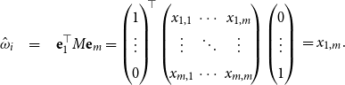 \begin{equation*}\begin{array}{@{}r@{\quad}l@{\quad}l}\hat{\omega}_i & = & {\textbf{e}}_1^\top M {\textbf{e}}_m =\left(\begin{matrix}1 \\\vdots \\0\\\end{matrix}\right)^{\!\!\top}\left(\begin{matrix}\!x_{1,1} & \cdots & x_{1,m}\!\\\!\vdots & \ddots & \vdots\! \\\!x_{m,1} & \cdots & x_{m,m}\!\end{matrix}\right)\left(\begin{matrix}0 \\\vdots \\1\\\end{matrix}\right)\\[4.5ex]\end{array}= x_{1,m}.\end{equation*}
Hence, to minimize the error, we update this entry in every matrix
 $M_\sigma$
that corresponds to a unigram
$M_\sigma$
that corresponds to a unigram
 $s_i= \sigma$
of a scored unigram phrase
$s_i= \sigma$
of a scored unigram phrase
 $(s_i,\omega_i)$
in our training set by this value, that is, we let
$(s_i,\omega_i)$
in our training set by this value, that is, we let
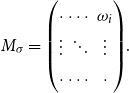 \begin{equation*}M_{\sigma} =\left(\begin{matrix}\cdot & \cdots & \omega_i\\\vdots & \ddots & \vdots \\\cdot & \cdots & \cdot\end{matrix}\right)\! .\end{equation*}
This way, we have initialized the word-to-matrix mapping such that it leads to perfect scores on all unigrams mentioned in the training set.
First Learning Step. After initialization, we consider bigram phrases. The predicted score
 $\hat{\omega}_i$
of a bigram phrase
$\hat{\omega}_i$
of a bigram phrase
 $s_i = \sigma\sigma'$
is now computed by
$s_i = \sigma\sigma'$
is now computed by
 \begin{equation}\hat{\omega}_i = {\textbf{e}}_1 M_{\sigma}M^{\prime}_{\sigma} {\textbf{e}}_m^\top =\left(\begin{matrix}1 \\\vdots \\0\\\end{matrix}\right)^{\!\!\!\!\top}\!\!\!\left(\begin{matrix}\!x_{1,1} & \cdots & x_{1,m}\!\\\!\vdots & \ddots & \vdots\! \\\!x_{m,1} & \cdots & x_{m,m}\!\end{matrix}\right)\!\!\!\left(\begin{matrix}\!y_{1,1} & \cdots & y_{1,m}\!\\\!\vdots & \ddots & \vdots\! \\\!y_{m,1} & \cdots & y_{m,m}\!\end{matrix}\right)\!\!\!\left(\begin{matrix}0 \\\vdots \\1\\\end{matrix}\right) =\left(\begin{matrix}x_{1,1} \\\vdots \\x_{1,m}\\\end{matrix}\right)^{\!\!\!\!\top}\!\!\!\left(\begin{matrix}y_{1,m} \\\vdots \\y_{m,m}\\\end{matrix}\right)= \displaystyle\sum_{j=1}^m x_{1,j}y_{j,m}.\end{equation}
We observe that for bigrams, multiplying the first row of the first matrix (row vector) with the last column of the second matrix (column vector) yields the score of the bigram phrase. Hence, as far as the scoring of unigrams and bigrams is concerned, only the corresponding row and column vectors are relevant – thanks to our specific choice of the vectors
 ${\unicode[Alpha]{x1D6C2}} = {\textbf{e}}_1$
and
${\unicode[Alpha]{x1D6C2}} = {\textbf{e}}_1$
and
 $\unicode[Beta]{x1D6C3} = {\textbf{e}}_m$
.
$\unicode[Beta]{x1D6C3} = {\textbf{e}}_m$
.
This observation justifies the next learning step: we use the unigrams and bigrams in the training set to learn optimal values for the relevant matrix entries only.
Second Learning Step. Using the entries obtained in the previous learning step for initialization, we finally repeat the optimization process, using the full training set and optimizing all the matrix values simultaneously, as described in the previous section.
7.2 Gradient descent for vector extraction with pre-trained vector embeddings
The type of learning method discussed here is different from the previous ones. As opposed to these, we are not aiming at a scoring model that assigns scalars to phrases, but want to associate phrases with vectors. This is particularly suitable for NLP tasks that require linguistic entities to be mapped into a vector space for comparison via distance or similarity measures. In such a setting, the training data consists of pairs
 $(s_i,{\textbf{v}}_i)$
, where
$(s_i,{\textbf{v}}_i)$
, where
 $s_i$
is a phrase and
$s_i$
is a phrase and
 ${\textbf{v}}_i$
the vector associated to it. Such training data can be obtained in different ways. One of the popular methods is to use the word2vec model (Mikolov et al. Reference Mikolov, Sutskever, Chen, Corrado and Dean2013b), in which a two-layer NN is trained to produce high-dimensional vectors for words. In this model, short phrases can also be considered as units and the model is trained to extract a vector representation for phrases as well as for words (Mikolov et al. Reference Mikolov, Sutskever, Chen, Corrado and Dean2013b).
${\textbf{v}}_i$
the vector associated to it. Such training data can be obtained in different ways. One of the popular methods is to use the word2vec model (Mikolov et al. Reference Mikolov, Sutskever, Chen, Corrado and Dean2013b), in which a two-layer NN is trained to produce high-dimensional vectors for words. In this model, short phrases can also be considered as units and the model is trained to extract a vector representation for phrases as well as for words (Mikolov et al. Reference Mikolov, Sutskever, Chen, Corrado and Dean2013b).
The model we train for this task is along the lines of Section 6.1. That is, given the word-to-matrix mapping
 $[\!\!\,[\cdot]\,\!\!]$
, we obtain the predicted vector
$[\!\!\,[\cdot]\,\!\!]$
, we obtain the predicted vector
 $\hat{{\textbf{v}}}_i$
for a phrase
$\hat{{\textbf{v}}}_i$
for a phrase
 $s_i = \sigma_1\ldots\sigma_k$
through the multiplication of its word matrices
$s_i = \sigma_1\ldots\sigma_k$
through the multiplication of its word matrices
 $[\!\!\,[\sigma_j]\,\!\!] \in \mathbb{R}^{m\times m}$
and the projection of the resulting matrix to the vector space
$[\!\!\,[\sigma_j]\,\!\!] \in \mathbb{R}^{m\times m}$
and the projection of the resulting matrix to the vector space
 $\mathbb{R}^{m}$
using a mapping vector
$\mathbb{R}^{m}$
using a mapping vector
 ${\unicode[Alpha]{x1D6C2}} \in \mathbb{R}^m$
as follows:
${\unicode[Alpha]{x1D6C2}} \in \mathbb{R}^m$
as follows:
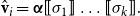 \begin{equation}\hat{{\textbf{v}}}_{i} = {\unicode[Alpha]{x1D6C2}} [\!\!\,[\sigma_1]\,\!\!] \ldots [\!\!\,[\sigma_k]\,\!\!].\end{equation}
We could now train the word matrices directly similar to the approach introduced in Section 7.1.1. However, we will exploit the fact that for every word
 $\sigma$
a pre-trained vector
$\sigma$
a pre-trained vector
 ${\textbf{v}}_\sigma$
is readily available and, as previous studies in DSMs have shown, semantic similarity between two words
${\textbf{v}}_\sigma$
is readily available and, as previous studies in DSMs have shown, semantic similarity between two words
 $\sigma$
and
$\sigma$
and
 $\sigma'$
correlates with smaller distances between their vector representations
$\sigma'$
correlates with smaller distances between their vector representations
 ${\textbf{v}}_\sigma$
and
${\textbf{v}}_\sigma$
and
 ${\textbf{v}}^{\prime}_\sigma$
(Padó and Lapata Reference Padó and Lapata2007; Mitchell and Lapata Reference Mitchell and Lapata2008; Turney and Pantel Reference Turney and Pantel2010). We want to preserve that information by making sure that closeness of
${\textbf{v}}^{\prime}_\sigma$
(Padó and Lapata Reference Padó and Lapata2007; Mitchell and Lapata Reference Mitchell and Lapata2008; Turney and Pantel Reference Turney and Pantel2010). We want to preserve that information by making sure that closeness of
 ${\textbf{v}}_\sigma$
and
${\textbf{v}}_\sigma$
and
 ${\textbf{v}}^{\prime}_\sigma$
entails similarity of
${\textbf{v}}^{\prime}_\sigma$
entails similarity of
 $[\!\!\,[\sigma]\,\!\!]$
and
$[\!\!\,[\sigma]\,\!\!]$
and
 $[\!\!\,[\sigma']\,\!\!]$
. To this end, in the learning algorithm, we let
$[\!\!\,[\sigma']\,\!\!]$
. To this end, in the learning algorithm, we let
 \begin{equation*}[\!\!\,[\sigma]\,\!\!] = {\textbf{v}}_\sigma \bf{T},\end{equation*}
where
 ${\bf T} \in \mathbb{R}^{m \times m \times m}$
is a shared third-order tensor and
${\bf T} \in \mathbb{R}^{m \times m \times m}$
is a shared third-order tensor and
 ${\textbf{v}}_\sigma {\bf T}$
yields the matrix M with
${\textbf{v}}_\sigma {\bf T}$
yields the matrix M with
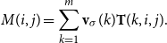 \begin{equation*}M(i,j)=\sum_{k=1}^m {\textbf{v}}_\sigma(k){\bf T}(k,i,j).\end{equation*}
Besides having the above-mentioned effect, the usage of a shared tensor significantly reduces the number of model parameters to be trained. Using a shared tensor in this way is inspired by Irsoy and Cardie (Reference Irsoy and Cardie2015).
T must produce suitable word matrices, which consequently result in vector representation of the corresponding phrase. Therefore, we train the tensor in a regression model. Stochastic gradient descent optimization is used to train the tensor T as a regression task to minimize the loss function defined as SSE, namely
 \begin{equation*}E_{T} = \sum_{i=1}^{N}||\hat{{\textbf{v}}}_i - {\textbf{v}}_{i}||_2^2.\end{equation*}
Note that
 $[\!\!\,[\sigma_1]\,\!\!] \ldots [\!\!\,[\sigma_k]\,\!\!]$
in Equation (2) is the compositional matrix representation of the compound, but since the training dataset is only available in vector space, we use a global mapping vector
$[\!\!\,[\sigma_1]\,\!\!] \ldots [\!\!\,[\sigma_k]\,\!\!]$
in Equation (2) is the compositional matrix representation of the compound, but since the training dataset is only available in vector space, we use a global mapping vector
 $\alpha$
to map the final matrix to a vector representation.
$\alpha$
to map the final matrix to a vector representation.
The output is to learn a composition function
 $\psi$
, which predicts the vector
$\psi$
, which predicts the vector
 $\hat{{\textbf{v}}}_i$
for a compound
$\hat{{\textbf{v}}}_i$
for a compound
 $s_i = \sigma_1\ldots\sigma_{k_i}$
through the multiplication of its word matrices
$s_i = \sigma_1\ldots\sigma_{k_i}$
through the multiplication of its word matrices
 $[\!\!\,[\sigma_j]\,\!\!] \in \mathbb{R}^{m\times m}$
, obtained from the trained tensor
$[\!\!\,[\sigma_j]\,\!\!] \in \mathbb{R}^{m\times m}$
, obtained from the trained tensor
 $\bf{T}$
, and the projection of the resulting matrix to the vector space
$\bf{T}$
, and the projection of the resulting matrix to the vector space
 $\mathbb{R}^{m}$
using the global mapping vector
$\mathbb{R}^{m}$
using the global mapping vector
 $\alpha \in \mathbb{R}^m$
as follows:
$\alpha \in \mathbb{R}^m$
as follows:
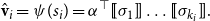 \begin{equation*}\hat{{\textbf{v}}}_{i} = \psi(s_i) = \alpha^\top [\!\!\,[\sigma_1]\,\!\!] \ldots [\!\!\,[\sigma_{k_i}]\,\!\!].\end{equation*}
Finally, the CMSM learns to compose the word matrix representations and predicts the vector representation of the compound by mapping the final compound matrix to the vector space.
8. Experiments
As discussed before, CMSMs can be used as alternative models to compositional VSMs in various NLP tasks. In this section, we conduct experiments to evaluate the performance of CMSMs on predicting compositionality. First, we investigate CMSMs on compositionality prediction of a sub-category of MWEs, that is, nominal compounds, and compare to popular baseline compositional VSMs. Then, considering sentiment analysis tasks, we study how well CMSMs capture sentiment composition of different types of short phrases.
8.1 Evaluation on fine-grained compositionality prediction
MWEs are short compounds with two or more words showing a range of semantic compositionality (semantic idiomaticity). The semantics of a compositional MWE can be understood from the meaning of its components such as graduate student, whereas the semantics of a non-compositional compounds cannot be predicted from the semantics of its parts, such as kick the bucket. The meaning of this compound is “to die,” which cannot be obtained from the meaning of kick and bucket (Baldwin and Kim Reference Baldwin and Kim2010). MWEs are of different types such as nominal and verbal MWEs. Predicting the degree of compositionality of MWEs is specially important in NLP applications such as phrase-based machine translation (Kordoni and Simova Reference Kordoni and Simova2014) and word sense disambiguation (Finlayson and Kulkarni Reference Finlayson and Kulkarni2011). Therefore, suitable models to capture the degree of semantic compositionality of MWEs are required for downstream applications. In this experiment, we evaluate the performance of several baseline CDSMs on predicting the degree of MWEs’ compositionality and compare them to CMSMs.
Baseline Compositional Distributional Semantic Models. Each model defines a composition function f over the constituent word vectors to predict the compound vector. Given two words
 $w_i$
and
$w_i$
and
 $w_j$
with associated vectors
$w_j$
with associated vectors
 ${\textbf{v}}_i \in \mathbb{R}^m$
and
${\textbf{v}}_i \in \mathbb{R}^m$
and
 ${\textbf{v}}_j \in \mathbb{R}^m$
, we evaluate the following baseline CDSMs:
${\textbf{v}}_j \in \mathbb{R}^m$
, we evaluate the following baseline CDSMs:
-
Weighted additive model: In this model, the predicted compound vector representation is obtained as the weighted sum of the constituent word vectors (Mitchell and Lapata Reference Mitchell and Lapata2008; Reddy et al. Reference Reddy, McCarthy and Manandhar2011), letting
where
\begin{equation*} \hat{{\textbf{v}}}_{ij} = f(w_i,w_j) = \lambda_1 {\textbf{v}}_{i} + \lambda_2 {\textbf{v}}_{j} \quad \text{ with } \quad \lambda_1+\lambda_2 = 1, \end{equation*}
$\lambda_1$
and
$\lambda_2$
are the weight coefficients.
-
Multiplicative model: In this model, the predicted compound vector representation is the element-wise product of the constituent word vectors (Mitchell and Lapata Reference Mitchell and Lapata2008; Reddy et al. Reference Reddy, McCarthy and Manandhar2011), that is,
\begin{equation*} \hat{{\textbf{v}}}_{ij} = f(w_i,w_j) = {\textbf{v}}_{i} \odot {\textbf{v}}_{j}. \end{equation*}
-
Polynomial regression model: In this model, to predict the compound representation
${\textbf{v}}_{ij}$
, the constituent word vectors are stacked together
$[{\textbf{v}}_i,{\textbf{v}}_j]$
and a polynomial function
$\psi$
is applied to them (Yazdani et al. Reference Yazdani, Farahmand and Henderson2015), yielding where
\begin{equation*} \hat{{\textbf{v}}}_{ij} = f(w_i,w_j) = \psi{([{\textbf{v}}_{i},{\textbf{v}}_{j}])}\theta, \end{equation*}
$\theta$
is the weight matrix to be trained, and
$\psi$
is the quadratic transformation applied to the input vectors.
\begin{equation*} \psi(x_1\ \cdots\ x_{2m}) = (x_1^2\ \cdots\ x_{2m}^2\ \ \, x_1x_2\ \cdots\ x_{2m-1}x_{2m}\ \ \, x_1\ \cdots\ x_{2m}) \end{equation*}
-
Feedforward NN: In this model, the constituent word vectors are stacked together as the input vector, and the input and output weight matrices are trained to predict the vector representation of the compound (Yazdani et al. Reference Yazdani, Farahmand and Henderson2015), defined by
where W and V are the input-to-hidden and hidden-to-output layer weight matrices to be trained and
\begin{equation*} \hat{{\textbf{v}}}_{ij} = f({\textbf{v}}_i,{\textbf{v}}_j) = \sigma([{\textbf{v}}_{i},{\textbf{v}}_{j}] W) V, \end{equation*}
$\sigma$
is a nonlinear function, such as the sigmoid function. The size of the hidden layer h in the network is set to 300.
-
Recurrent NN (RNN): In this model, the input word vectors are fed into the network sequentially. The hidden state at time step t is computed by
where g is an activation function, such as
\begin{equation*} \textbf{h}_t = g({\textbf{v}}_t U + \textbf{h}_{t-1} W + \textbf{b}), \end{equation*}
$\textit{tanh}$
, to introduce nonlinearity. The hidden state
$\textbf{h}_{t-1}$
from previous time step is combined with the current input
${\textbf{v}}_t$
and a bias
$\textbf{b}$
. The new hidden state
$\textbf{h}_{t}$
that we computed will then be fed back into the RNN cell together with the next input and this process continues until the last input feeds into the network. Inputs are the word vectors of the compounds in a sequence. The size of the hidden layer is set to 300. We only require the output of the last time step T in the sequence, and therefore we pass the last hidden layer
$\textbf{h}_T$
through a linear layer to generate the predicted compound vector representation via where V is the shared weight matrix of the linear layer.
\begin{equation*} \hat{{\textbf{v}}}_{ij} = \textbf{h}_T V + \textbf{c}, \end{equation*}
-
Compositional Matrix-Space Model: this model has been introduced in Section 7.2.


LSTM networks have been developed to deal with long input sequences of variable length and vanishing gradients (Hochreiter and Schmidhuber Reference Hochreiter and Schmidhuber1997; Yu et al. Reference Yu, Si, Hu and Zhang2019). However, our investigations focus on sequences of length just two, so plain RNNs do not suffer from the vanishing gradient problem. Thus, we refrain from separately reporting on LSTMs, as their performance does not significantly differ from that of plain RNNs.
For all models tested, the predicted compound vectors are compared to the true (target) vector representation of the compounds through the similarity measurements. Note that the constituent word vectors and the target compound vectors are obtained by training the vector embeddings of all words and compounds using word2vec (Mikolov et al. Reference Mikolov, Chen, Corrado and Dean2013a) and fastText (Bojanowski et al. Reference Bojanowski, Grave, Joulin and Mikolov2017) on English Wikipedia dump 2018Footnote g as our corpus. It has been shown that these models capture the semantics of short compositional phrases as well as words (Mikolov et al. Reference Mikolov, Sutskever, Chen, Corrado and Dean2013b). We report the results of word2vec and fastText separately.
Training Data. For supervised models (CMSM, polynomial regression model, Feedforward NN, and RNN), we fit the composition function f using supervised learning methods to capture the compositional representation of the compounds. Therefore, as described in Section 7.2, we create a training dataset from frequent two-word compounds extracted from our corpus Wikipedia dump 2018. We create two training datasets for our experiments: one dataset consists of compounds with associated target representations obtained from word2vec, and the other includes the same compounds with associated target representations obtained from fastText. We limit our experiments to bigrams as they are the most basic compositional structures and to respect the evaluation datasets standard. We assume the majority of compounds are compositional and train the compositional models on each training dataset separately. From each created training data, we extracted about 0.1 of the data as the development set.
Evaluation Datasets. Finally, we use two recent gold standard evaluation datasets which reflect the compositionality judgments of MWEs to evaluate all compositional models:
-
Farahmand15 Footnote h (Farahmand et al. Reference Farahmand, Smith and Nivre2015) provides 1,042 English noun–noun (N–N) compounds (bigrams) extracted from Wikipedia which were annotated with a non-compositionality degree between 0 (fully compositional) to 1 (fully non-compositional) using crowdsourcing. Each compound was annotated by four annotators for binary non-compositionality judgments, and the average of annotations was considered as the final score of the compound which is a value from
$\{0,0.25,0.5,0.75,1\}$
. -
Reddy++ Footnote i (Ramisch et al. Reference Ramisch, Cordeiro, Zilio, Idiart and Villavicencio2016; Reddy et al. Reference Reddy, McCarthy and Manandhar2011) provides 180 English N–N and A–N compounds (bigrams) with real-valued compositionality degree ranging from 0 (fully non-compositional) to 5 (fully compositional) obtained from crowdsourcing and averaged over around 10–20 annotators per compound. The dataset contains 143 N–N and 37 A–N compounds.
The vector representation of bigrams in the evaluation datasets is obtained from word2vec and fastText for examining the learned compositional models.
Experimental Setting and Results. In the experiments with word2vec, some compounds of the datasets are not available in the word embeddings. Therefore, to test each model we consider 800 compounds from the Farahmand15 dataset and 148 compounds from the Reddy++ dataset. The size of the training and development set are 7692 and 854 compounds, respectively, and fixed for all models. In the experiments with fastText, all compounds of the Farahmand15 and the Reddy++ datasets are included in fastText and therefore, we test each model on the whole dataset. The size of the training and development set are 11,566 and 1156 compounds, respectively, and fixed for all models. The batch size for the training is set to
 $b=10$
. The learning rate is adapted experimentally for each model.
$b=10$
. The learning rate is adapted experimentally for each model.
We apply early stopping by computing the loss value of the development set to prevent overfitting. If the absolute difference of development loss in two consecutive iterations is lower than the threshold of
 $\epsilon=10^{-5}$
, we stop the training. Once the model is trained, we evaluate the performance of the trained model on both test datasets. The tensor
$\epsilon=10^{-5}$
, we stop the training. Once the model is trained, we evaluate the performance of the trained model on both test datasets. The tensor
 $\bf{T}$
in the CMSM is initialized with Gaussian distribution
$\bf{T}$
in the CMSM is initialized with Gaussian distribution
 $\mathcal{N}(0,0.01)$
. The size of all vectors is set to 300 in both experiments with word2vec and fastText. We report the average results over 15 runs.
$\mathcal{N}(0,0.01)$
. The size of all vectors is set to 300 in both experiments with word2vec and fastText. We report the average results over 15 runs.
To measure the closeness (proximity) between the predicted compound representations using CDSMs and the true (target) representations of compounds, we compute cosine similarity as well as the loss between the two representations. Cosine similarity computes the cosine between the predicted composed vector and the true vector representation of the compound. To obtain the loss, we compute the squared error loss (SE loss) between the predicted and the true vector representation of the compound being sensitive to small errors. We expect a high loss value for non-compositional compounds as the composition functions are not able to capture their representations (Yazdani et al. Reference Yazdani, Farahmand and Henderson2015). Then, we compute the linear relationship between the computed similarity values and the compositionality judgments from the test datasets. For this purpose, we use the Pearson coefficient value r where a linear correlation between the values is computed ranging from
 $-1$
to 1 with higher values showing more correlation between the predicted and gold standard values.
$-1$
to 1 with higher values showing more correlation between the predicted and gold standard values.
Tables 4 and 5 show the average Pearson correlation coefficient r between the predicted similarity values and the gold standard values in each dataset for different compositional models. Table 4 shows the results of the word2vec word embedding, and Table 5 shows the results of the fastText word embeddings. Compositionality prediction of models is shown in two ways as described before. First, if a method captures the compositional representation of the compounds, the cosine similarity between the predicted and true representations has a higher value, otherwise the cosine similarity has a low value. Therefore, the cosine similarity column in both tables shows the result of Pearson correlation value between the cosine similarity of the representation and the gold standard values in the test datasets, which are normalized between
 $-1$
(non-compositional) and 1 (compositional) compounds. Second, if a method captures the compositional representation of the compounds, following Yazdani et al. (Reference Yazdani, Farahmand and Henderson2015), the loss value between the predicted and true representation of a compositional compound must be low and close to 0, otherwise it is a high value. Therefore, the squared error loss (SE loss) column in the tables shows the result of the correlation of the loss value (between the representations) with the gold standard values in the test datasets, which are normalized to 0 (fully compositional) and 1 (fully non-compositional). The tables demonstrate that the two measures provide very similar results.
$-1$
(non-compositional) and 1 (compositional) compounds. Second, if a method captures the compositional representation of the compounds, following Yazdani et al. (Reference Yazdani, Farahmand and Henderson2015), the loss value between the predicted and true representation of a compositional compound must be low and close to 0, otherwise it is a high value. Therefore, the squared error loss (SE loss) column in the tables shows the result of the correlation of the loss value (between the representations) with the gold standard values in the test datasets, which are normalized to 0 (fully compositional) and 1 (fully non-compositional). The tables demonstrate that the two measures provide very similar results.
Table 4. Pearson value r for compositionality prediction using word2vec
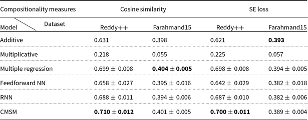
Table 5. Pearson value r for compositionality prediction using fastText
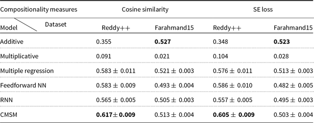
We report the best results of the additive and multiplicative models obtained by adapting
 $\lambda_1$
and
$\lambda_1$
and
 $\lambda_2$
(ranging from 0 to 1 with step size of
$\lambda_2$
(ranging from 0 to 1 with step size of
 $0.1$
) in these models. As we observe in both tables, the multiplicative model is not powerful enough to predict compositionality. These results are in line with the results in the work by Yazdani et al. (Reference Yazdani, Farahmand and Henderson2015). The CMSM is trained to predict the compositionality better than other models in the Reddy++ dataset in both tables, which means that CMSM gives a higher loss value and lower cosine similarity to non-compositional compounds. Moreover, the CMSM converges to its best model in fewer training iterations on average. The number of training iterations for each supervised compositional model to reach its optimal performance is shown in Table 6.
$0.1$
) in these models. As we observe in both tables, the multiplicative model is not powerful enough to predict compositionality. These results are in line with the results in the work by Yazdani et al. (Reference Yazdani, Farahmand and Henderson2015). The CMSM is trained to predict the compositionality better than other models in the Reddy++ dataset in both tables, which means that CMSM gives a higher loss value and lower cosine similarity to non-compositional compounds. Moreover, the CMSM converges to its best model in fewer training iterations on average. The number of training iterations for each supervised compositional model to reach its optimal performance is shown in Table 6.
Table 6. Average number of training iterations for each supervised model trained using word2vec and fastText

As is observed, CMSM converges faster than NN in both word embeddings and faster than multiple regression in the fastText embedding, which shows an advantage of the model in convergence speed with the same vector dimensionality. It is not significantly slower than other models. The different iteration numbers in the two-word embeddings are due to the different learning rate adapted to obtain the best models on the word embeddings. Various parameters such as the training data and vector embeddings impact the performance of the models. Therefore, in our experiments, we used the same training data and vector embeddings for all models to obtain a more reliable indication regarding the relative performance of the models.
In the Farahmand15 dataset, the additive model outperforms CMSM while in the Reddy++ dataset, the CMSM outperforms the additive model considerably. We speculate that this is because the Reddy++ is a dataset with much more fine-grained values and CMSMs tend to be more accurate in predicting the nuanced values than other models. Moreover, Reddy++ contains A–N and N–N compounds as opposed to Farahmand15, which contains only noun compounds. Therefore, we conclude that CMSMs can learn to capture the compositionality degree of the combination of different compound types and predict the compositionality of A–N compounds better than the studied compositional models. Figures 3 and 4 present sample compounds from Reddy++ and Farahmand15 datasets with predicted compositionality degrees by different models. In both figures, we analyze the prediction of models that are trained using fastText embeddings and cosine similarity is the compositionality measure showing the scores. As can be seen in Figure 3, we choose different A–N and N–N compounds from Reddy++ with varying gold standard scores from 0, that is, wet blanket to 1, that is, insurance company. The relationship between gold and predicted scores in the figure describes the Pearson correlation value presented in Table 5. Compared to the competitive additive model, CMSM follows an increasing trend in the predicted scores. It assigns a slightly higher score to the A–N compound mental disorder than to cellular phone. All models fail to predict the score of the A–N compound private eye, which can be due to the lower frequency of its subwords in the given Wikipedia training corpus. Multiplicative model fails to follow the increasing trend in the predicted scores as opposed to other models.
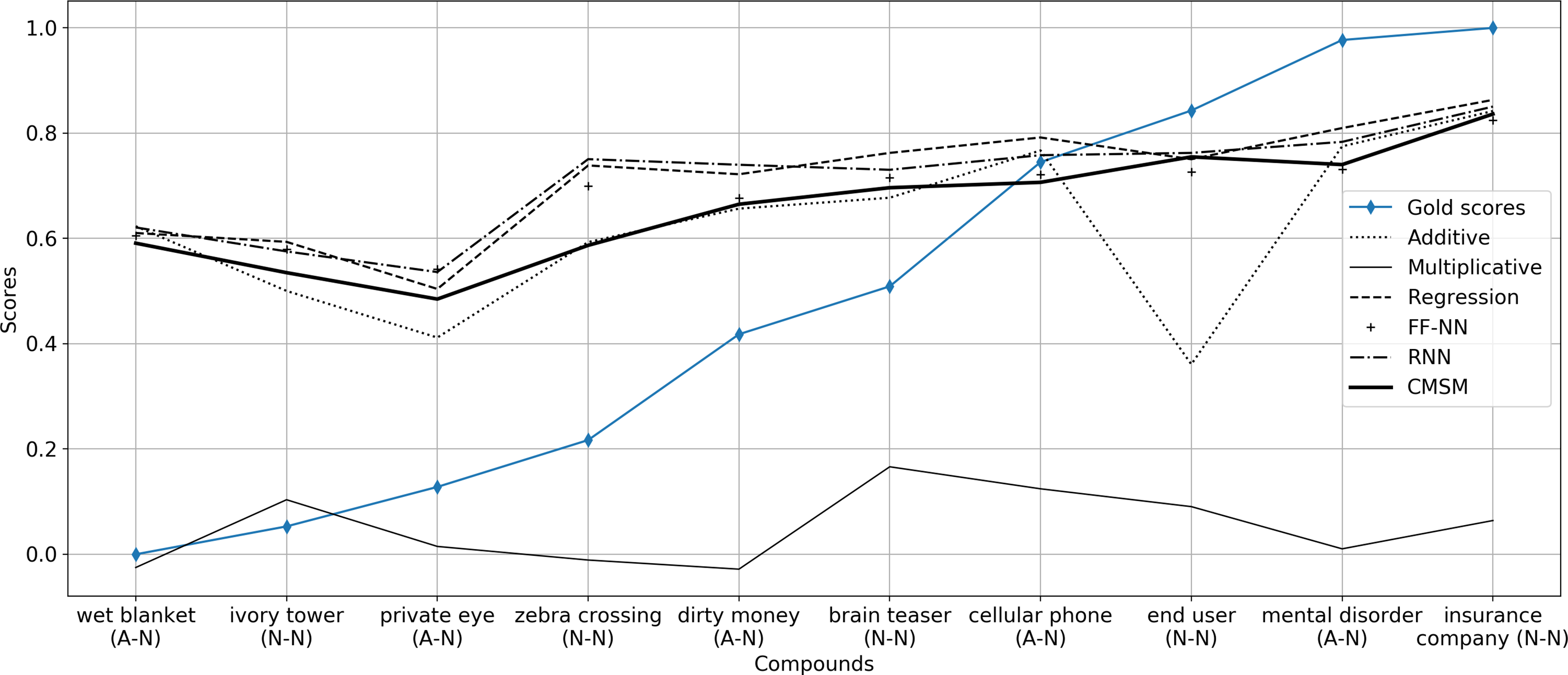
Figure 3. Sample compounds from Reddy++ with predicted average compositionality scores by different models and gold standard scores. Results of fastText embeddings are reported. Gold standard scores are between 0 (non-compositional) and 1 (fully compositional). A, adjective; N, noun; FF, Feedforward.
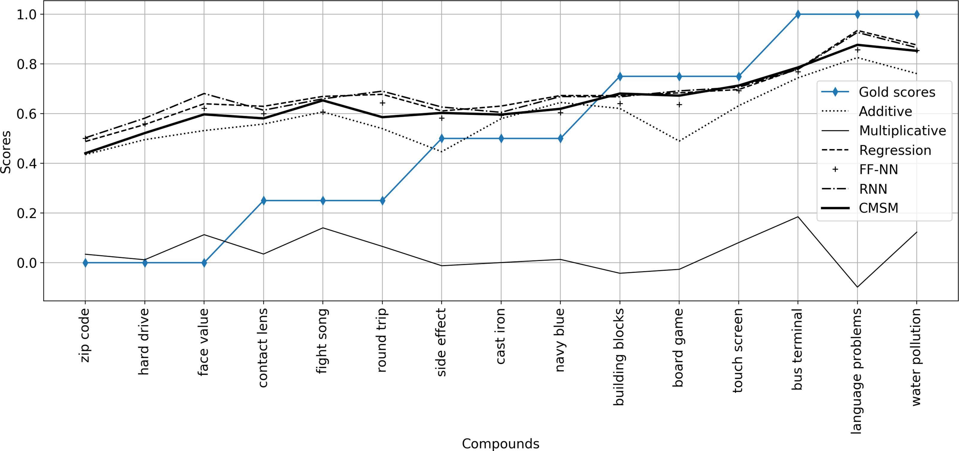
Figure 4. Sample compounds from Farahmand15 with predicted average compositionality scores by different models and gold standard scores. Results of fastText embeddings are reported. Gold standard scores are between 0 (non-compositional) and 1 (fully compositional). FF, Feedforward.
We randomly selected 15 compounds from the Farahmand15 dataset. Figure 4 confirms the increasing trend in the predicted scores by all models except by the multiplicative model. In general, compounds with the same gold standard score are not assigned to the same score in regression tasks. The high difference in some compounds, such as in face value and zip code, could be due to different frequencies and distributions of their subwords, resulting in different compositionality prediction. In most cases, CMSM predictions are closer than the additive model’s predictions, for example, in building block, navy blue and touch screen compounds.
Note that while this work is similar to the very recent work by Cordeiro et al. (Reference Cordeiro, Villavicencio, Idiart and Ramisch2019), our corpus size and parameter settings for training word embeddings, such as embedding size, are different. Therefore, their results are not directly comparable to our results and we repeated the experiment. Higher performance reported in Cordeiro et al. (Reference Cordeiro, Villavicencio, Idiart and Ramisch2019) is due to a much bigger training corpus of word and compound embeddings and larger embedding size, which consequently consumes memory. They only experiment on unsupervised approaches as opposed to our work, in which we evaluate supervised approaches as well.
According to these results, we can conclude that a CMSM can be trained to capture the semantic compositionality of compounds more efficiently than baseline VSMs. Moreover, CMSMs are sensitive to syntactic properties such as the word order of the compound which affects the meaning of complex expressions. The results suggest that matrix multiplication should be considered instead of additive models as the composition operation to capture semantic composition along long texts.
8.2 Evaluation on fine-grained sentiment analysis
Sentiment analysis is one of the most popular tasks in NLP. The task is to determine the sentiment polarity and intensity of a text, for example, “a very good movie” indicates a positive sentiment about the movie while “a very bad movie” carries a negative sentiment. With the increasing importance of review websites for marketing, a lot of research has been done in sentiment analysis to automatically extract the opinion of people about a certain topic. In general, the task of sentiment analysis is to rate the sentiment of a text using either binary classification (negative, positive) or multiple classes (negative, positive, neutral) with intensities (weak, medium, extreme), the latter being called fine-grained sentiment analysis. The sentiment score can be also computed as a real-valued score in a continuous interval showing the polarity and intensity of the text, which then can be mapped to classification problem by discretization.
Sentiment analysis can be applied to a single word or texts of varying length including short and long texts. There are several aspects which must be considered when analyzing complex texts. First, different types of constituents and functional words such as negators, adjectives, adverbs, and intensifiers affect the total sentiment of the text differently. Second, a different order of the words results in a different sentiment score. Yessenalina and Cardie (Reference Yessenalina and Cardie2011) showed an application of CMSMs in compositional sentiment analysis task (see an example in Figure 5) and how it captures compositionality and the above properties in this task. They proposed a supervised machine learning technique for learning CMSMs in sentiment analysis of short texts. The proposed method learns a matrix representation for each word which captures compositionality properties of the language.
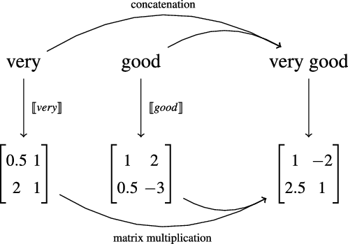
Figure 5. Sentiment composition of a short phrase with matrix multiplication as a composition operation in CMSMs.
In high dimensional matrix-space models, each dimension is a model parameter to be estimated in the optimization problem. Some parameters might not be relevant to the problem, and the number of parameters is usually higher than the size of the data. Parameters in a high-dimensional space are also dependent on each other. Due to these properties, several local optima in the objective surface can be found during the optimization of the objective function. In such a situation, the solution depends heavily on initialization to provide a better starting point for exploration of optimal points and avoid immediate local optima. Furthermore, training steps can be designed carefully to help effective exploration and exploitation.
Training CMSMs using machine learning techniques yields a type of word embedding for each word, which is a low-dimensional real-valued matrix. Similar to word vectors in VSMs, each word matrix is supposed to contain syntactic and semantic information about the word. Since we consider the task of sentiment analysis, word embeddings must be trained to contain sentiment-related information.
In the following, we train CMSMs to capture the sentiment score of compositional phrases. We apply our learning approach introduced in Section 7.1.2 to train CMSMs. Word matrices are initialized in two ways: random initialization from the Normal distribution and identity matrices plus a noise value from the Normal distribution. Our approach with the introduced informed initialization and two learning steps (see Section 7.1.2) is called gradual gradient descent-based matrix-space models (Grad-GMSM) in which the word matrices are initialized randomly. The same approach with the identity plus a noise value as the initialization for matrices is called Grad-GMSM+IdentityInit. We conduct several experiments with two different datasets and discuss the results in detail.
Datasets. We use the following datasets for our experiment purposes:
-
SCL-OPP (Sentiment Composition Lexicon with Opposing Polarity Phrases) Footnote j : this dataset consists of 602 unigrams, 311 bigrams, and 265 trigrams that have been taken from a corpus of tweets, and annotated with real-valued sentiment scores in the interval
$[-1,+1]$
by Kiritchenko and Mohammad (Reference Kiritchenko and Mohammad2016b). Each multi-word phrase contains at least one negative word and one positive word. The dataset contains different noun and verb phrases. The frequency of polarities is as per Table 7.Table 7. Phrase polarities and their occurrence frequencies in the SCL-OPP dataset
-
MPQA (Multi-Perspective Question Answering) opinion corpus Footnote k : this dataset contains newswire documents annotated with phrase-level polarity and intensity. We extracted the annotated verb and noun phrases from the corpus documents, obtaining 9501 phrases. We removed phrases with low intensity similar to Yessenalina and Cardie (Reference Yessenalina and Cardie2011). The levels of polarities and intensities, their translation into numerical values, and their occurrence frequency are as per Table 8.
Table 8. Phrase polarities and intensities in the MPQA corpus, their translation into sentiment scores and their occurrence frequency

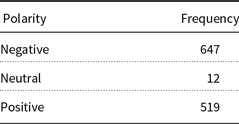

8.2.1 Evaluation on SCL-OPP
The purpose of this experiment is to investigate the performance of the CMSMs in predicting the sentiment composition of phrases that contain words with opposing polarities. The sentiment value of words (unigrams) is given for training the CMSM. In the first part, we compare the results to the results obtained from word2vec embeddings in the work by Kiritchenko and Mohammad (Reference Kiritchenko and Mohammad2016b). In the second part, we explore different choices of dimensionality in learning CMSMs.
For the purposes of the first experiment, we set the dimension of matrices to
 $m=200$
to be able to compare the results with those reported in Kiritchenko and Mohammad (Reference Kiritchenko and Mohammad2016b) as well as
$m=200$
to be able to compare the results with those reported in Kiritchenko and Mohammad (Reference Kiritchenko and Mohammad2016b) as well as
 $m = 5$
, and number of iterations to
$m = 5$
, and number of iterations to
 $T=400$
. We choose
$T=400$
. We choose
 $m=5$
based on practical experiments, and as we will show in Table 11, by increasing the dimensions from 2 to 5 better performance could be obtained, however, with higher dimensions we did not observe significant improvement in the performance of the model. Word matrices are initialized with an identity matrix plus a noise from Gaussian distribution
$m=5$
based on practical experiments, and as we will show in Table 11, by increasing the dimensions from 2 to 5 better performance could be obtained, however, with higher dimensions we did not observe significant improvement in the performance of the model. Word matrices are initialized with an identity matrix plus a noise from Gaussian distribution
 $\mathcal{N}(0,0.01)$
as it is also suggested in previous works (Socher et al. Reference Socher, Huval, Manning and Ng2012; Maillard and Clark Reference Maillard and Clark2015). We use the sentiment value of unigrams to initialize the corresponding element in the word matrices. The learning rate
$\mathcal{N}(0,0.01)$
as it is also suggested in previous works (Socher et al. Reference Socher, Huval, Manning and Ng2012; Maillard and Clark Reference Maillard and Clark2015). We use the sentiment value of unigrams to initialize the corresponding element in the word matrices. The learning rate
 $\eta$
in gradient descent is set to
$\eta$
in gradient descent is set to
 $0.017$
and
$0.017$
and
 $0.001$
for dimension 200 and 5, respectively. We use the Pearson correlation coefficient r for performance evaluation, which measures the linear correlation between the predicted and the target sentiment value of phrases. Pearson coefficient value ranges from
$0.001$
for dimension 200 and 5, respectively. We use the Pearson correlation coefficient r for performance evaluation, which measures the linear correlation between the predicted and the target sentiment value of phrases. Pearson coefficient value ranges from
 $-1$
to 1 with higher values showing more correlation between the predicted and target values.
$-1$
to 1 with higher values showing more correlation between the predicted and target values.
We first report the results for training only trigrams in the dataset since training bigrams does not train all the elements in word matrices. When bigrams are trained using the mapping vectors
 ${\textbf{e}}_1$
and
${\textbf{e}}_1$
and
 ${\textbf{e}}_m$
, only the first row of the first word matrix and the last column of the second word matrix are trained and other elements of the matrices remain fixed. This can be seen in Equation (1). Then, we combine trigrams and bigrams as our training set and apply our regular training procedure on the whole dataset. We consider it important that the learned model generalizes well to phrases of variable length; hence, we consider the training of one model per phrase length not conducive. Rather, we argue that training CMSM can and should be done independent of the length of phrases, by ultimately using the combination of different length phrases for training and testing, given the sentiment value of unigrams.
${\textbf{e}}_m$
, only the first row of the first word matrix and the last column of the second word matrix are trained and other elements of the matrices remain fixed. This can be seen in Equation (1). Then, we combine trigrams and bigrams as our training set and apply our regular training procedure on the whole dataset. We consider it important that the learned model generalizes well to phrases of variable length; hence, we consider the training of one model per phrase length not conducive. Rather, we argue that training CMSM can and should be done independent of the length of phrases, by ultimately using the combination of different length phrases for training and testing, given the sentiment value of unigrams.
We apply a 10-fold cross-validation process on the training data as follows: eight folds are used as training set, one fold as validation set, and one fold as test set. We average over 10 repeated runs to obtain the final results. At each run, folds are selected randomly and we report the best results obtained from early stopping in T iterations. As a measure of statistical dispersion, we report the standard deviation of Pearson values in 10 repeated runs.
Kiritchenko and Mohammad (Reference Kiritchenko and Mohammad2016b) study different patterns of sentiment composition in phrases. They analyze the efficacy of baseline and supervised methods on these phrases, and the effect of different features such as POS tags, pre-trained word vector embeddings, and sentiment score of unigrams in learning sentiment regression. Table 9 shows the results of different methods for training the trigrams. As baseline, they evaluate the last unigram of the phrase (Row 1), POS tags of the phrase (Row 2), and most polar unigram of the phrase (Row 3) to predict the overall sentiment score of the phrase. As a supervised method, they apply RBF kernel-based SVR (RBF-SVR). In RBF-SVR, different set of features are evaluated on predicting real-valued sentiment scores. Row 8 considers the following features which give the best results: all unigrams (uni), their sentiment scores (sent. score), POS tags (POS), and concatenation of unigram embeddings (emb(conc)). Results show that concatenation of unigram embeddings as the composition operation outperforms average of unigram embeddings (emb(ave)) and maximal embeddings (emb(max)). The embeddings are obtained from word2vec (Mikolov et al. Reference Mikolov, Chen, Corrado and Dean2013a). They analyze the results for bigrams and trigrams separately. Our approach does not use information extracted from other resources (such as pre-trained word embedding) nor POS tagging techniques, that is, we perform a light-weight training with fewer features, which can be considered as an advantage of CMSMs. As it is shown in Table 9, we observe better performance of Grad-GMSM on trigram phrases (Rows10) over baseline methods and emb(ave) as the composition operation (Row 7). We also obtained similar results with significantly lower dimensions (Row 9), which still outperforms the described models. In contrast, vector concatenation as the composition operation (Rows 6 and 8) outperforms our model by transforming the embeddings to a different space (to a higher dimensional space). Matrix multiplication remains in the same space and this introduces an advantage of matrix multiplication over vector concatenation. Table 10 presents the sentiment score of some representative phrases with different POS predicted by CMSMs and their gold standard scores. On average, the predicted results correlate with the gold standard results. A small discrepancy can be observed, for example, best winter break is expected to be more positive than happy tears and tired but happy, but it is predicted as less positive.
Table 9. Performance comparison for different methods in SCL-OPP dataset considering only trigram phrases
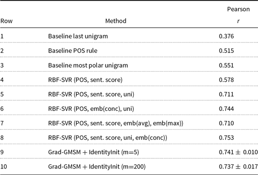
Table 10. Example phrases with average sentiment scores on 10-fold cross-validation and different POS tags. A, adjective; N, noun; V, verb; &, and; D, determiner
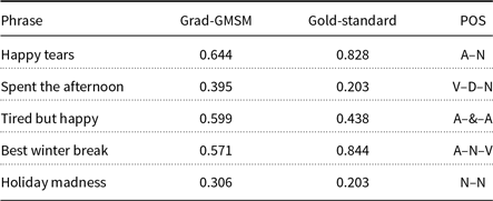
Finally, we repeated the experiments on the Grad-GMSM+IdentityInit model with values of m (i.e., different numbers of dimensions), and using the whole dataset (i.e., bigram and trigram phrases). Note that unigrams are only included for initialization of the training step and we excluded them from the validation and test sets. The noise values are drawn from Gaussian distribution
 $\mathcal{N}(0,0.01)$
. Number of iterations are set to
$\mathcal{N}(0,0.01)$
. Number of iterations are set to
 $T=400$
. The learning rate
$T=400$
. The learning rate
 $\eta$
is set to
$\eta$
is set to
 $0.01$
and
$0.01$
and
 $0.001$
for the first and second steps, respectively. For each dimension number, we take the average of five runs of 10-fold cross validation. As shown in Table 11, the results improve only marginally when increasing m over several orders of magnitude. Also the average number of required iterations remains essentially the same, except for
$0.001$
for the first and second steps, respectively. For each dimension number, we take the average of five runs of 10-fold cross validation. As shown in Table 11, the results improve only marginally when increasing m over several orders of magnitude. Also the average number of required iterations remains essentially the same, except for
 $m=1$
, which does not exploit the matrix properties and performs like the bag-of-words model. We see that – as opposed to VSMs – good performance can be achieved already with a very low number of dimensions. By increasing the dimensionality, the number of parameters to train grows, which leads the model to get stuck in local optima in the objective surface.
$m=1$
, which does not exploit the matrix properties and performs like the bag-of-words model. We see that – as opposed to VSMs – good performance can be achieved already with a very low number of dimensions. By increasing the dimensionality, the number of parameters to train grows, which leads the model to get stuck in local optima in the objective surface.
Table 11. Performance comparison for different dimensions of matrices in the complete SCL-OPP dataset (i.e., considering bigrams and trigrams for the experiment)
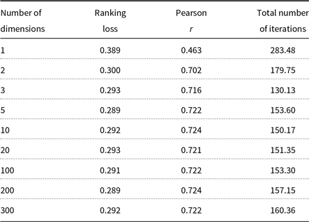
8.2.2 Evaluation on MPQA
The purpose of this experiment is to evaluate the performance of CMSMs in predicting the sentiment value of phrases of variable length. We compare the performance of our proposed method to two closely related approaches introduced by Yessenalina and Cardie (Reference Yessenalina and Cardie2011), called Matrix-space OLogReg+BowInit, and by Irsoy and Cardie (Reference Irsoy and Cardie2015), called mRNN. We choose these two approaches because the first learning method focuses on training the CMSMs. The latter method, inspired by CMSMs, generalizes the model and incorporates multiplicative interaction of matrices for compositionality in RRNs in the task of sentiment analysis. First, we explain these methods and their relevance to our work. Then, we discuss the obtained results in different methods.
Yessenalina and Cardie (Reference Yessenalina and Cardie2011) propose a model to predict an ordinal sentiment score (e.g., label 0 for highly negative sentiment, 1 for medium negative, 2 for neutral, and so on) for a given phrase. The model learns an interval for each sentiment label. Therefore, the model parameters to optimize are the word matrices as well as a set of threshold values (also called constraints), which indicate the intervals for sentiment classes as they convert sentiment classes to ordinal labels. Word matrices are initialized in two ways: random initialization using the normal distribution, and BOWs initialization. In the latter case, first a Bag-of-Words OLogReg (BOW-OLogReg) model is trained on the same dataset in which each word in the BOWs model learns a scalar weight using OLogReg. Then, a specific element of matrices is initialized with the learned weights from BOW-OLogReg. They apply OLogReg to train word matrices and optimize the threshold values by maximizing the probability of predicting the sentiment interval of given phrases in the dataset or minimizing the negative log of the probability. To avoid ill-conditioned matrices, they add a projection step to matrices after each training iteration by shrinking all singular values of matrices close to one. The trained model with random initialization is called Matrix-space OLogReg+RandInit and the one with BOW initialization is called Matrix-space OLogReg+BowInit. The latter model outperforms the random initialization of the matrix-space model. They argue that the learning problem for CMSMs is a non-convex optimization problem, that is, the objective function of optimization problem can get stuck at local optima in the high dimensional matrix space. Therefore, the model must be initialized and trained carefully to avoid getting stuck in local optima.
We relax the non-convexity issue in our proposed learning method by introducing a specific initialization and gradual stochastic gradient descent learning strategy. Our results in the sentiment analysis task demonstrate the effectiveness of the proposed initialization and training strategy in obtaining better performance of the trained model than existing approaches. Moreover, Yessenalina and Cardie (Reference Yessenalina and Cardie2011) propose a model for ordinal sentiment scale prediction and address the optimization problem using the OLogReg method with constraints on sentiment intervals. As opposed to their work, we directly address a sentiment regression task. Therefore, our learning method does not need to constrain the sentiment scores to certain intervals, and thus, the number of parameters to learn reduces to only word matrices.
Inspired by CMSMs, Irsoy and Cardie (Reference Irsoy and Cardie2015) proposed mRNN to train the CMSMs. In mRNN, a multiplicative interaction between the input vector and the previous hidden layer in a RNN is introduced using a shared third-order tensor
 ${\bf T} \in \mathbb{R}^{m \times m \times m}$
. At each time step, the input word vector
${\bf T} \in \mathbb{R}^{m \times m \times m}$
. At each time step, the input word vector
 ${\textbf{v}} \in \mathbb{R}^m$
is multiplied with the weight tensor
${\textbf{v}} \in \mathbb{R}^m$
is multiplied with the weight tensor
 $\bf{T}$
, which results in a matrix M of size
$\bf{T}$
, which results in a matrix M of size
 $m \times m$
. Then the resulting matrix is multiplied with the previous hidden layer
$m \times m$
. Then the resulting matrix is multiplied with the previous hidden layer
 $\textbf{h}_{t-1}$
to finally obtain the current hidden layer at time step t. Therefore, if the current hidden layer of a RNN is defined by
$\textbf{h}_{t-1}$
to finally obtain the current hidden layer at time step t. Therefore, if the current hidden layer of a RNN is defined by
 \begin{equation*}\textbf{h}_t = g({\textbf{v}}_t U + \textbf{h}_{t-1} W + \textbf{b}),\end{equation*}
then the mRNN computes the current hidden layer according to
 \begin{equation*}\textbf{h}_t = g({\textbf{v}}_t U + \textbf{h}_{t-1} W + {\textbf{v}}_t^\top {\bf T} \textbf{h}_{t-1} + \textbf{b} ),\end{equation*}
where in both equations, U and W are the shared weight matrices for input-to-hidden and hidden-to-hidden layers, respectively, and
 $\textbf{b}$
is the bias of the network. g is a nonlinear activation function, such as tanh function.
$\textbf{b}$
is the bias of the network. g is a nonlinear activation function, such as tanh function.
 ${\textbf{v}}_t$
is the specific input word at time t, while
${\textbf{v}}_t$
is the specific input word at time t, while
 $\textbf{h}_t$
is the result of the current hidden layer. This means that the multiplicative relation between the input and the previous hidden layer is added to the current hidden layer computation. Thus, by introducing the shared tensor
$\textbf{h}_t$
is the result of the current hidden layer. This means that the multiplicative relation between the input and the previous hidden layer is added to the current hidden layer computation. Thus, by introducing the shared tensor
 $\bf{T}$
, they incorporate multiplicative interaction in matrix space to RNNs using the term
$\bf{T}$
, they incorporate multiplicative interaction in matrix space to RNNs using the term
 $ {\textbf{v}}_t^\top {\bf T} \textbf{h}_{t-1}$
. They use pre-trained word vectors of dimension
$ {\textbf{v}}_t^\top {\bf T} \textbf{h}_{t-1}$
. They use pre-trained word vectors of dimension
 $m=300$
from word2vec (Mikolov et al. Reference Mikolov, Sutskever, Chen, Corrado and Dean2013b) as the input to their network. They show that the interactive multiplication outperforms the additive interaction in vector space in RNNs in the task of compositional sentiment analysis. Moreover, in this way, the number of parameters to learn in the CMSMs is reduced. Furthermore, as opposed to the approach for compositionality via multiplicative interaction introduced by Socher et al. (Reference Socher, Perelygin, Wu, Chuang, Manning, Ng and Potts2013), parse trees are not required. Inspired by this model, we introduce a shared third-order tensor to the model and train the tensor to obtain word matrix representations by multiplying any word vector with the trained tensor. Then, word matrices are further utilized for capturing compositionality of phrases in CMSMs using matrix multiplication. Moreover, similar to this work, we aim at capturing compositionality through sequential multiplication without using parse trees. However, as opposed to this work, we do not introduce nonlinear functions in our proposed approach as we aim to keep the original characteristics of CMSMs.
$m=300$
from word2vec (Mikolov et al. Reference Mikolov, Sutskever, Chen, Corrado and Dean2013b) as the input to their network. They show that the interactive multiplication outperforms the additive interaction in vector space in RNNs in the task of compositional sentiment analysis. Moreover, in this way, the number of parameters to learn in the CMSMs is reduced. Furthermore, as opposed to the approach for compositionality via multiplicative interaction introduced by Socher et al. (Reference Socher, Perelygin, Wu, Chuang, Manning, Ng and Potts2013), parse trees are not required. Inspired by this model, we introduce a shared third-order tensor to the model and train the tensor to obtain word matrix representations by multiplying any word vector with the trained tensor. Then, word matrices are further utilized for capturing compositionality of phrases in CMSMs using matrix multiplication. Moreover, similar to this work, we aim at capturing compositionality through sequential multiplication without using parse trees. However, as opposed to this work, we do not introduce nonlinear functions in our proposed approach as we aim to keep the original characteristics of CMSMs.
As described above, word matrices are initialized in two ways. Our proposed approach in Section 7.1.2 with random initialization of matrices from the Normal distribution is called Grad-GMSM, and with identity matrices plus a noise value from the Normal distribution is called Grad-GMSM+IdentityInit. To assess the effect of our gradual two-step training method, we study the impact of different types of matrix initialization and compare the results of Grad-GMSM against those obtained by random initialization followed by a single training phase where the full matrices were optimized (RandInit-GMSM).
We apply a 10-fold cross-validation process on the training data as follows: eight folds are used as training set, one fold as validation set, and one fold as test set. The initial number of iterations in the first learning and second learning steps is set to
 $T=400$
each, but we stop iterating when we obtain the minimum ranking loss
$T=400$
each, but we stop iterating when we obtain the minimum ranking loss
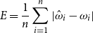 \begin{equation*} E = \frac{1}{n}\sum_{i=1}^n |\hat{\omega}_i - \omega_i|\end{equation*}
on the validation set. Finally, we record the ranking loss of the obtained model for the test set. The learning rate
 $\eta$
of the first and second training steps was adapted experimentally to
$\eta$
of the first and second training steps was adapted experimentally to
 $0.01$
and
$0.01$
and
 $0.001$
, respectively. The dimension of matrices is set to
$0.001$
, respectively. The dimension of matrices is set to
 $m=3$
to be able to compare our results to the related approaches described by Yessenalina and Cardie (Reference Yessenalina and Cardie2011) and Irsoy and Cardie (Reference Irsoy and Cardie2015). However, we study the impact of the number of dimensions on the CMSM performance.
$m=3$
to be able to compare our results to the related approaches described by Yessenalina and Cardie (Reference Yessenalina and Cardie2011) and Irsoy and Cardie (Reference Irsoy and Cardie2015). However, we study the impact of the number of dimensions on the CMSM performance.
Table 12 compares the result of our model to the explained Yessenalina and Cardie (Reference Yessenalina and Cardie2011)’s models and Irsoy and Cardie (Reference Irsoy and Cardie2015)’s model in the matrix space. As we observe, Grad-GMSM+IdentityInit obtains a significantly lower ranking loss than previously proposed methods and our Grad-GMSM approach.
Table 12. Ranking loss of compared methods
By comparing Grad-GMSM+IdentityInit with Grad-GMSM, we also observe faster convergence, since the lowest ranking loss of Grad-GMSM+IdentityInit is obtained after
 $114.55$
number of training iterations on average. In Grad-GMSM, the lowest ranking loss happens on average after
$114.55$
number of training iterations on average. In Grad-GMSM, the lowest ranking loss happens on average after
 $161.85$
number of training iterations. RandInit-GMSM is not able to converge to its best model in T iterations.
$161.85$
number of training iterations. RandInit-GMSM is not able to converge to its best model in T iterations.
Table 13 shows the sentiment scores of some example phrases trained using these two methods. As shown in the table, the two approaches’ results coincide regarding the order of basic phrases: the score of “very good” is greater than “good” (and both are positive) and the score of “very bad” is lower than “bad” (and both are negative). Also, “not good” is characterized as negative by both approaches. On the other hand, there are significant differences between the two approaches: for example, our approach characterizes the phrase “not bad” as mildly positive while Yessenalina and Cardie (Reference Yessenalina and Cardie2011)’s approach associates a negative score to it, the same discrepancy occurs for “not very bad”. Intuitively, we tend to agree more with our method’s verdict on these phrases.
In general, our findings confirm those of Yessenalina and Cardie (Reference Yessenalina and Cardie2011): “very” seems to intensify the value of the subsequent word, while the “not” operator does not just flip the sentiment of the word after it but also dampens the sentiment of the words gradually. On the other hand, the scores of phrases starting with “not very” defy the assumption that the described effects of these operators can be combined in a straightforward way. Adverbs and negators in natural language play an important role in determining the sentiment score of phrases. Our results showed that multiplicative interaction in CMSMs captures the effect of adverbs and negators on the sentiment score when composed with a phrase. Figure 6 provides a more comprehensive selection of phrases and their predicted scores by our approach. We obtained the range of sentiment scores by taking the minimum and maximum values predicted in the 10-fold cross-validation. We obtained an average of
 $\omega(\textit{very very good})= 0.98$
, which is greater than “very good”, and
$\omega(\textit{very very good})= 0.98$
, which is greater than “very good”, and
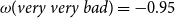 $\omega(\textit{very very bad})= -0.95$
lower than “very bad”. Therefore, we can also consider “very very” as an intensifier operator. Moreover, we observe that the average score of
$\omega(\textit{very very bad})= -0.95$
lower than “very bad”. Therefore, we can also consider “very very” as an intensifier operator. Moreover, we observe that the average score of
 $\omega(\textit{not really good}) = -0.34$
is not equal to the average score of
$\omega(\textit{not really good}) = -0.34$
is not equal to the average score of
 $\omega(\textit{really not good}) = -0.58$
, which demonstrates that the matrix-based compositionality operation shows sensitivity to word orders, arguably reflecting the meaning of phrases better than any commutative operation could.
$\omega(\textit{really not good}) = -0.58$
, which demonstrates that the matrix-based compositionality operation shows sensitivity to word orders, arguably reflecting the meaning of phrases better than any commutative operation could.
Table 13. Frequent phrases with average sentiment scores
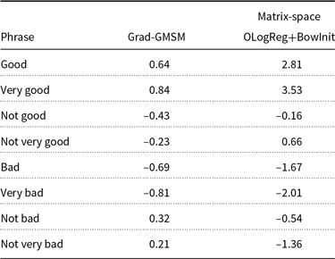

Figure 6. The order of sentiment scores for sample phrases (trained on MPQA corpus).
Although the training data consists of only the values of Table 8, we consider a regression method for training CMSMs. Thus, the training of the model is done in a way that sentiment scores for phrases with more extreme intensity might yield real values greater than
 $+1$
or lower than
$+1$
or lower than
 $-1$
, since we do not constrain the sentiment scores to
$-1$
, since we do not constrain the sentiment scores to
 $[-1,+1]$
. Moreover, in our experiments we observed that no extra precautions were needed to avoid ill-conditioned matrices or abrupt changes in the scores while training.
$[-1,+1]$
. Moreover, in our experiments we observed that no extra precautions were needed to avoid ill-conditioned matrices or abrupt changes in the scores while training.
To observe the effect of a higher number of dimensions on our approach, we repeated the experiments for Grad-GMSM+IdentityInit with
 $m=50$
, and observed a ranking loss of
$m=50$
, and observed a ranking loss of
 $e=0.3092$
 $\pm \:$
 $0.011$
(i.e., virtually the same as for
$0.011$
(i.e., virtually the same as for
 $m=3$
) and almost similar values for the number of training iterations
$m=3$
) and almost similar values for the number of training iterations
 $T=122$
confirming the observation of Yessenalina and Cardie (Reference Yessenalina and Cardie2011), that increasing the number of dimensions does not significantly improve the prediction quality of the obtained model.
$T=122$
confirming the observation of Yessenalina and Cardie (Reference Yessenalina and Cardie2011), that increasing the number of dimensions does not significantly improve the prediction quality of the obtained model.
In Table 14, we study the time cost required for training CMSMs in the studied training data (SCL–OPP and MPQA) and with two different dimensionalities (5 and 200). Note that we report the time cost for 10-fold cross-validation. Results show the advantage of smaller dimensionality of CMSMs in faster convergence.
Table 14. Time cost for training CMSMs with different dimensionality and datasets. Time is reported in minutes
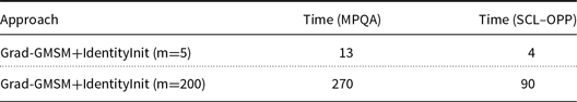
9. Discussion, conclusion, and future work
We have introduced a generic model for compositionality in language where matrices are associated with tokens and the matrix representation of a token sequence is obtained by iterated matrix multiplication. On the theoretical side, we have given algebraic and structural plausibility indications in favor of this choice. We have shown that the proposed model is expressive enough to cover and combine distributional and symbolic aspects of natural language, and simulate both numeric and symbolic approaches to language in contrast to VSMs.
On the practical side, we have studied the behavior of CMSMs along different aspects (e.g. dimensionality) experimentally. According to experimental investigations in Section 14, CMSMs are a promising framework to model task-specific semantic compositionality such as compositional sentiment analysis and compositionality prediction of short phrases. The proposed approach for learning CMSMs in compositional sentiment analysis provides an informed initialization for a better starting point for exploration of optimal points and a gradual gradient descent-based learning strategy to avoid immediate local optima. It outperforms previous approaches to CMSMs in this task. Moreover, matrix product as the composition operation in CMSMs outperforms vector averaging as the composition operation in VSMs in the same task and on a special dataset consisting of opposing polarity phrases. Small dimensionality and independence from extra preprocessing of the training data (e.g., POS tagging) can be put forward as the advantages of CMSMs in compositional sentiment analysis.
In the compositionality prediction task, CMSMs outperform several vector-space baseline models on a gold standard dataset consisting of N–N and A–N compounds. Results show that CMSMs are more accurate in predicting the compositionality of A–N compounds than the studied VSMs. However, CMSMs do not outperform vector addition on another gold standard dataset of N–N compounds, which is in contrast to the theoretical studies showing superiority of matrix product over vector addition. We speculate that other aspects than compositionality play an important role in such tasks, such as the approach to create the underlying gold standard dataset, and the distribution of semantic representation of individual words in the space.
We have seen strong evidence that CMSMs embed relevant information in considerably fewer dimensions than in VSMs on these specific tasks, which gives a clear advantage in terms of computational cost and storage in training. Certainly, while CMSMs overcome certain limitations of VSMs, they may still inherit some of their foundational weaknesses (cf. Ježek Reference Ježek2016). We are aware that experiments have been only done on short length sequences, and further investigation is needed for examining the suitability of CMSMs for longer texts, such as sentences.
Matrix multiplication on long sequences introduces the vanishing or exploding gradient problem and can cause the final matrix to contain extremely small values. Hence, when updating word matrices in the gradient descent algorithm, small values are obtained from the derivative of the loss function with respect to a word matrix M, which may not update the word matrix values adequately. Therefore, mechanisms are needed to avoid this issue when training CMSMs on long sequences. Moreover, when CMSMs are trained on long sequences in a specific task, such as sentiment analysis, not all words contain task-specific information. A method could be introduced to learn attention weights for words and give more weights to those words that carry the relevant information, for instance, sentiment-carrying words in sentiment analysis.
Furthermore, due to associativity, matrix multiplication cannot capture all syntactic information of a long sentence. Therefore, certain linguistic effects (like a-posteriori disambiguation) cannot be modeled via associative mappings. Thus, we might equip CMSMs with nonlinear functions to introduce non-associativity to the CMSMs and resolve word sense disambiguation problems in natural language. For instance, one could apply some sort of sigmoid function to the output of matrix multiplications for any given two matrices in a sequence. The resulting matrix can then be multiplied with the next word matrix followed again by application of a nonlinear mapping. Thus, another avenue of further research is to generalize from the linear approach, very much in line with the current trend in deep learning techniques. For instance, when designing deep neural architectures, we can incorporate word matrices and multiplicative composition instead of additive vector composition into hidden layers of the network to obtain intermediate representation for phrase matrices. That is, weight matrices in the hidden layers of a network are replaced with third-order weight tensors, which results in matrix-space operations. A similar idea has been proposed by Chung et al. (Reference Chung, Wang and Bowman2018) who incorporate CMSMs into tree-structured LSTMs to capture multiplicative interaction in the composition of words to sentences for natural language understanding.
Recently, contextualized word representation models, such as ELMo (Peters et al. Reference Peters, Neumann, Iyyer, Gardner, Clark, Lee and Zettlemoyer2018) and BERT (Devlin et al. Reference Devlin, Chang, Lee and Toutanova2019), have shown state-of-the-art performance in downstream NLP tasks. These models have been trained on pre-training objectives, such as masked language modeling, using huge text corpora. However, they need to be fine-tuned on downstream NLP tasks using task-specific training data. Since CMSMs can be also trained using similar task-specific datasets, we suggest that when dealing with NLP tasks where compositionality plays an important role, such as in phrase-based statistical machine translation (Weller et al. Reference Weller, Cap, Müller, Schulte im Walde and Fraser2014; Kordoni and Simova Reference Kordoni and Simova2014), a comparative analysis of contextualized and non-contextualized representation models in capturing the compositional meaning of phrases would be helpful to choose the best approach for phrase-level compositional representation. CMSMs capture the nuances of compositional phrase meaning and training these models needs lower computational cost, which could be useful in situations where limited computational resources are available.
Overall, this work demonstrates that CMSMs compose attractive theoretical features and practical behavior, which strongly suggest CMSMs as a suitable model of semantic compositionality in downstream NLP applications. Moreover, recent research in psycholinguistics has focused on assessing the cognitive plausibility of DSMs and word embeddings in VSMs. We can similarly argue for the psychological plausibility of CMSMs, which is presented in Appendix C. However, we leave the justification of these models as a separate research work since systematic analysis of these models in psychologically related tasks, such as semantic priming, is needed.
As future work, we will explore how to train task-independent CMSMs to capture the distributional representation of words similar to non-contextualized distributional VSMs such as word2vec and even contextualized language representation models such as pre-trained BERT (Devlin et al. Reference Devlin, Chang, Lee and Toutanova2019) in which distinct embeddings of a word can be obtained when occurring in different contexts. One immediate advantage of employing distributional matrix-space models is that matrix multiplication is an operation which is most natural, plausible on several levels, word-order-sensitive, and allows for a dynamic composition of word matrices to longer phrases and even sentences. However, if and how semantic information can be embedded in fewer dimensions than BERT or word2vec still needs to be investigated.
Another interesting line of research on CMSMs is to investigate the performance of CMSMs in capturing compositionality in other languages such as German, where individual words can be combined to make compounds leading to infinite number of German compounds. However, suitable preprocessing techniques for compound splitting would be needed for this purpose (Weller et al. Reference Weller, Cap, Müller, Schulte im Walde and Fraser2014).
Acknowledgements
This research is partially supported by the German Research Foundation (DFG) within the Research Training Group QuantLA (GRK 1763) and by the Federal Ministry of Education and Research of Germany BMBF through the Center for Scalable Data Analytics and Artificial Intelligence (ScaDS.AI).
A. CMSMs capture compositional vector-space models
A.1 Vector addition
As a simple (and arguably the most straight-forward) basic model for semantic composition, vector addition has been proposed. Thereby, tokens
 $\sigma$
get assigned (usually high-dimensional) vectors
$\sigma$
get assigned (usually high-dimensional) vectors
 ${\textbf{v}}_\sigma$
and to obtain a representation of the meaning of a sequence
${\textbf{v}}_\sigma$
and to obtain a representation of the meaning of a sequence
 $s=\sigma_1\ldots\sigma_k$
, the vector sum of the vectors associated with the constituent tokens is calculated:
$s=\sigma_1\ldots\sigma_k$
, the vector sum of the vectors associated with the constituent tokens is calculated:
 ${\textbf{v}}_s=\sum_{i=1}^k{\textbf{v}}_{\sigma_i}$
.
${\textbf{v}}_s=\sum_{i=1}^k{\textbf{v}}_{\sigma_i}$
.
This kind of composition operation is subsumed by CMSMs; suppose in the original model, a token
 $\sigma$
gets assigned the vector
$\sigma$
gets assigned the vector
 ${\textbf{v}}_\sigma$
, then by defining
${\textbf{v}}_\sigma$
, then by defining
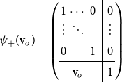 \begin{equation*}\psi_+({\textbf{v}}_\sigma) = \left(\begin{array}{ccc|c}1 & \cdots & 0\ \ & \ 0 \\[-1mm]\vdots & \ddots & & \ \vdots \\0 & & 1 \ \ & \ 0 \\\hline& {\textbf{v}}_\sigma & & \ 1 \\\end{array}\right)\end{equation*}
(mapping n-dimensional vectors to
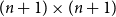 $(n+1)\times(n+1)$
matrices) as well as
$(n+1)\times(n+1)$
matrices) as well as
 \begin{equation*}\chi_+(M) = (M(m,1) \quad M(m,2) \quad \cdots \quad M(m,m-1))\end{equation*}
(that is, given a matrix M, extract the lowest row omitting the last entry), we obtain for a sequence
 $s=\sigma_1\ldots\sigma_k$
 \begin{equation*}\chi_+(\psi_+({\textbf{v}}_{\sigma_1})\ldots\psi_+({\textbf{v}}_{\sigma_k}))={\textbf{v}}_{\sigma_1} + \ldots + {\textbf{v}}_{\sigma_k} = {\textbf{v}}_s.\end{equation*}
Proof. The correspondence is a direct consequence of the equality
 $\psi_+({\textbf{v}}_{\sigma_1})\ldots\psi_+({\textbf{v}}_{\sigma_k})=\psi_+({\textbf{v}}_{\sigma_1} + \ldots + {\textbf{v}}_{\sigma_k})$
which we prove by induction over k. For
$\psi_+({\textbf{v}}_{\sigma_1})\ldots\psi_+({\textbf{v}}_{\sigma_k})=\psi_+({\textbf{v}}_{\sigma_1} + \ldots + {\textbf{v}}_{\sigma_k})$
which we prove by induction over k. For
 $k=1$
, the claim is trivial. For
$k=1$
, the claim is trivial. For
 $k>1$
, we have
$k>1$
, we have
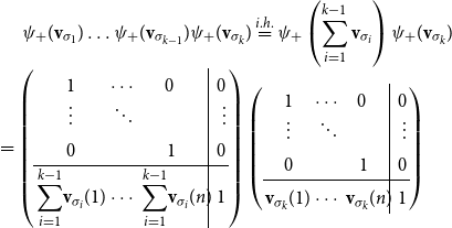 $\psi_+({\textbf{v}}_{\sigma_1})\ldots\psi_+({\textbf{v}}_{\sigma_{k-1}})\psi_+({\textbf{v}}_{\sigma_k})\stackrel{i.h.}{=}\psi_+\left(\displaystyle\sum_{i=1}^{k-1}{\textbf{v}}_{\sigma_i}\right)\psi_+({\textbf{v}}_{\sigma_k})\\ =\left(\begin{array}{c@{\ }c@{\ }c|@{\ }r} 1 & \cdots & 0\ & \ \ 0 \\[-1mm] \vdots & \ddots & & \vdots \\ 0 & & 1 & 0 \\\hline \displaystyle\sum_{i=1}^{k-1}\!{\textbf{v}}_{\sigma_i}(1) & \cdots & \displaystyle\sum_{i=1}^{k-1}\!{\textbf{v}}_{\sigma_i}(n)\!\!\! & 1 \\ \end{array}\right) \left(\begin{array}{c@{\ }c@{\ }c|@{\ }r} 1 & \cdots & 0\ & \ \ 0 \\[-1mm] \vdots & \ddots & & \vdots \\ 0 & & 1 & 0 \\\hline {\textbf{v}}_{\sigma_k}(1) & \cdots & {\textbf{v}}_{\sigma_k}(n)\!\!\! & 1 \\ \end{array}\right)$
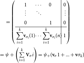 $=\left(\begin{array}{c@{}c@{}c|@{\ }r} 1 & \cdots & 0\ & \ \ 0 \\[-1mm] \vdots & \ddots & & \vdots \\ 0 & & 1 & 0 \\\hline \displaystyle\sum_{i=1}^{k}\!{\textbf{v}}_{\sigma_i}(1) & \cdots & \displaystyle\sum_{i=1}^{k}\!{\textbf{v}}_{\sigma_i}(n)\!\!\! & 1 \\ \end{array}\right)\\[5pt] = \psi+\left(\sum\limits^{k}_{i=1} \textbf{V}_\sigma i\right)=\psi_+(\textbf{v}_\sigma 1+...+\textbf{v}\sigma_{k})$
q.e.d.
$=\left(\begin{array}{c@{}c@{}c|@{\ }r} 1 & \cdots & 0\ & \ \ 0 \\[-1mm] \vdots & \ddots & & \vdots \\ 0 & & 1 & 0 \\\hline \displaystyle\sum_{i=1}^{k}\!{\textbf{v}}_{\sigma_i}(1) & \cdots & \displaystyle\sum_{i=1}^{k}\!{\textbf{v}}_{\sigma_i}(n)\!\!\! & 1 \\ \end{array}\right)\\[5pt] = \psi+\left(\sum\limits^{k}_{i=1} \textbf{V}_\sigma i\right)=\psi_+(\textbf{v}_\sigma 1+...+\textbf{v}\sigma_{k})$
q.e.d.
A.2 Component-wise multiplication
On the other hand, the Hadamard product (also called entry-wise product, denoted by
 $\odot$
) has been proposed as an alternative way of semantically composing token vectors.
$\odot$
) has been proposed as an alternative way of semantically composing token vectors.
Using a different encoding into matrices, CMSMs can simulate this type of composition operation as well. By letting
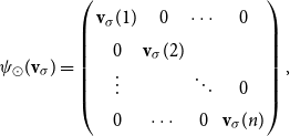 \begin{equation*}\psi_\odot({\textbf{v}}_\sigma) = \left(\begin{array}{cccc}{\textbf{v}}_\sigma(1) & 0 & \cdots & 0 \\0 & {\textbf{v}}_\sigma(2) & & \\\vdots & & \ddots & 0 \\0 & \cdots & 0 & {\textbf{v}}_\sigma(n)\\\end{array}\right),\end{equation*}
as well as
 \begin{equation*}\chi_\odot(M) = (M(1,1) \quad M(2,2) \quad \cdots \quad M(m,m))\end{equation*}
(i.e.,
 $\chi_\odot$
extracts the values of M’s diagonal), we obtain an
$\chi_\odot$
extracts the values of M’s diagonal), we obtain an
 $n\times n$
matrix representation such that for any sequence
$n\times n$
matrix representation such that for any sequence
 $s=\sigma_1\ldots\sigma_k$
holds
$s=\sigma_1\ldots\sigma_k$
holds
 \begin{equation*}\chi_\odot(\psi_\odot({\textbf{v}}_{\sigma_1})\ldots\psi_\odot({\textbf{v}}_{\sigma_k}))= {\textbf{v}}_{\sigma_1} \odot \ldots \odot {\textbf{v}}_{\sigma_k} = {\textbf{v}}_s.\end{equation*}
Proof. The correspondence is a direct consequence of the equality
 $\psi_\odot({\textbf{v}}_{\sigma_1})\ldots\psi_\odot({\textbf{v}}_{\sigma_k})=\psi_\odot({\textbf{v}}_{\sigma_1} \odot \ldots \odot {\textbf{v}}_{\sigma_k})$
which we prove by induction on k. For
$\psi_\odot({\textbf{v}}_{\sigma_1})\ldots\psi_\odot({\textbf{v}}_{\sigma_k})=\psi_\odot({\textbf{v}}_{\sigma_1} \odot \ldots \odot {\textbf{v}}_{\sigma_k})$
which we prove by induction on k. For
 $k=1$
, the claim is trivial. For
$k=1$
, the claim is trivial. For
 $k>1$
, we have
$k>1$
, we have
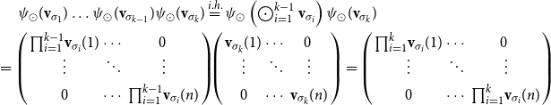 $\psi_\odot({\textbf{v}}_{\sigma_1})\ldots\psi_\odot({\textbf{v}}_{\sigma_{k-1}})\psi_\odot({\textbf{v}}_{\sigma_k})\stackrel{i.h.}{=}\psi_\odot\left(\bigodot_{i=1}^{k-1}{\textbf{v}}_{\sigma_i}\right)\psi_\odot({\textbf{v}}_{\sigma_k})\\ =\left(\begin{array}{c@{\ }c@{\ }c} \prod_{i=1}^{k-1}\!{\textbf{v}}_{\sigma_i}(1) & \cdots & 0\ \\[-1mm] \vdots & \ddots & \vdots \\ 0 & \cdots & \prod_{i=1}^{k-1}\!{\textbf{v}}_{\sigma_i}(n)\\ \end{array}\right)\!\! \left(\begin{array}{c@{\ }c@{\ }c} {\textbf{v}}_{\sigma_k}(1) & \cdots & 0\ \\[-1mm] \vdots & \ddots & \vdots \\ 0 & \cdots & {\textbf{v}}_{\sigma_k}(n) \\ \end{array}\right)= \left(\begin{array}{c@{\ }c@{\ }c} \prod_{i=1}^{k}\!{\textbf{v}}_{\sigma_i}(1) & \cdots & 0\ \\[-1mm] \vdots & \ddots & \vdots \\ 0 & \cdots & \prod_{i=1}^{k}\!{\textbf{v}}_{\sigma_i}(n) \end{array}\right)$
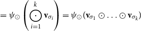 $\displaystyle = \psi_\odot\left(\bigodot_{i=1}^{k}{\textbf{v}}_{\sigma_i}\right) = \psi_\odot({\textbf{v}}_{\sigma_1} \odot \ldots \odot {\textbf{v}}_{\sigma_k})$
 $\left.\right.$
 $\left.\right.$
q.e.d.
$\left.\right.$
q.e.d.
A.3 Holographic reduced representations
Holographic reduced representations as introduced by Plate (Reference Plate1995) can be seen as a refinement of convolution products with the benefit of preserving dimensionality: given two vectors
 ${\textbf{v}}_1,{\textbf{v}}_2\in \mathbb{R}^n$
, their circular convolution product
${\textbf{v}}_1,{\textbf{v}}_2\in \mathbb{R}^n$
, their circular convolution product
 ${\textbf{v}}_1\circledast {\textbf{v}}_2$
is again an n-dimensional vector
${\textbf{v}}_1\circledast {\textbf{v}}_2$
is again an n-dimensional vector
 ${\textbf{v}}_3$
defined by
${\textbf{v}}_3$
defined by
 \begin{equation*}{\textbf{v}}_3(i+1) = \sum_{k=0}^{n-1} {\textbf{v}}_1(k+1)\cdot{\textbf{v}}_2((i-k \mod n)+1)\end{equation*}
for
 $0\leq i \leq n-1$
. Now let
$0\leq i \leq n-1$
. Now let
 $\psi_\circledast({\textbf{v}})$
be the
$\psi_\circledast({\textbf{v}})$
be the
 $n\times n$
matrix M with
$n\times n$
matrix M with
 \begin{equation*}M(i,j)={\textbf{v}}((j-i \mod n)+1).\end{equation*}
In the three-dimensional case, this would result in
 \begin{equation*}\psi_\circledast({\textbf{v}}(1)\quad {\textbf{v}}(2)\quad {\textbf{v}}(3)) = \left(\begin{array}{ccc}{\textbf{v}}(1) & {\textbf{v}}(2) & {\textbf{v}}(3) \\{\textbf{v}}(3) & {\textbf{v}}(1) & {\textbf{v}}(2) \\{\textbf{v}}(2) & {\textbf{v}}(3) & {\textbf{v}}(1) \\\end{array}\right).\end{equation*}
Figure A1 illustrates the computation of circular convolution operation as a compressed outer product of two vectors.
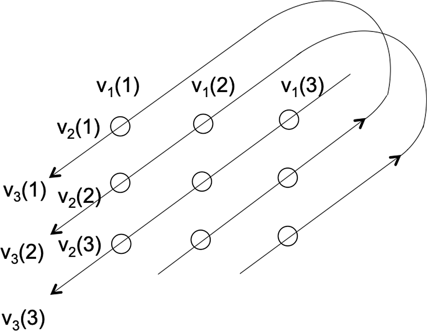
Figure A1. Circular convolution operation on two three-dimensional vectors
 ${{\textbf{v}}_1}$
and
${{\textbf{v}}_1}$
and
 ${{\textbf{v}}_2}$
. Illustration adapted from Plate (Reference Plate1995).
${{\textbf{v}}_2}$
. Illustration adapted from Plate (Reference Plate1995).
Furthermore, let
 \begin{equation*}\chi_\circledast(M)= (M(1,1)\quad\cdots\quad M(1,n))\end{equation*}
that is,
 $\chi_\circledast$
extracts the first row of M. Then we obtain, for any sequence
$\chi_\circledast$
extracts the first row of M. Then we obtain, for any sequence
 $s=\sigma_1\ldots\sigma_k$
, the desired correspondence
$s=\sigma_1\ldots\sigma_k$
, the desired correspondence
 \begin{equation*}\chi_\circledast(\psi_\circledast({\textbf{v}}_{\sigma_1})\ldots\psi_\circledast({\textbf{v}}_{\sigma_k}))= {\textbf{v}}_{\sigma_1} \circledast \ldots \circledast {\textbf{v}}_{\sigma_k} = {\textbf{v}}_s.\end{equation*}
Proof. We first show the following claim
 $(*)$
: for any
$(*)$
: for any
 ${\textbf{v}}_1,{\textbf{v}}_2 \in \mathbb{R}^n$
holds
${\textbf{v}}_1,{\textbf{v}}_2 \in \mathbb{R}^n$
holds
 $\psi_\circledast({\textbf{v}}_1\circledast {\textbf{v}}_2) = \psi_\circledast({\textbf{v}}_1) \psi_\circledast({\textbf{v}}_2)$
. To this end, let
$\psi_\circledast({\textbf{v}}_1\circledast {\textbf{v}}_2) = \psi_\circledast({\textbf{v}}_1) \psi_\circledast({\textbf{v}}_2)$
. To this end, let
 ${\textbf{v}}_3 = {\textbf{v}}_1\circledast {\textbf{v}}_2$
and
${\textbf{v}}_3 = {\textbf{v}}_1\circledast {\textbf{v}}_2$
and
 $N = \psi_\circledast({\textbf{v}}_3)$
, furthermore, let
$N = \psi_\circledast({\textbf{v}}_3)$
, furthermore, let
 $N_1=\psi_\circledast({\textbf{v}}_1)$
and
$N_1=\psi_\circledast({\textbf{v}}_1)$
and
 $N_2=\psi_\circledast({\textbf{v}}_2)$
as well as
$N_2=\psi_\circledast({\textbf{v}}_2)$
as well as
 $N' = N_1N_2$
. Then
$N' = N_1N_2$
. Then
 \begin{equation*}N(i,j)= {\textbf{v}}_3((j-i \mod n)+1)= \sum_{k=0}^{n-1} {\textbf{v}}_1(k+1)\cdot{\textbf{v}}_2(((j-i \mod n)-k \mod n)+1)\end{equation*}
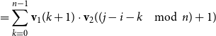 \begin{equation*}= \sum_{k=0}^{n-1} {\textbf{v}}_1(k+1)\cdot{\textbf{v}}_2((j-i-k \mod n)+1)\end{equation*}
as well as
 \begin{equation*}N'(i,j)= \sum_{\ell=1}^n N_1(i,\ell)\cdot N_2(\ell,j)= \sum_{\ell=1}^n {\textbf{v}}_1((\ell-i \mod n)+1)\cdot {\textbf{v}}_2((j-\ell \mod n)+1)\end{equation*}
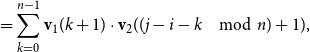 \begin{equation*}= \sum_{k=0}^{n-1} {\textbf{v}}_1(k+1)\cdot{\textbf{v}}_2((j-i-k \mod n)+1),\end{equation*}
where, in the last step, we substituted
 $\ell$
by
$\ell$
by
 $k+i \mod n$
and reordered the sum. Hence, we have shown that all entries of N and N coincide and therefore
$k+i \mod n$
and reordered the sum. Hence, we have shown that all entries of N and N coincide and therefore
 $\psi_\circledast({\textbf{v}}_1\circledast {\textbf{v}}_2) = N' = N = \psi_\circledast({\textbf{v}}_1) \psi_\circledast({\textbf{v}}_2)$
, proving
$\psi_\circledast({\textbf{v}}_1\circledast {\textbf{v}}_2) = N' = N = \psi_\circledast({\textbf{v}}_1) \psi_\circledast({\textbf{v}}_2)$
, proving
 $(*)$
.
$(*)$
.
Now we proceed to show the original statement, which is a direct consequence of the equality
 $\psi_\circledast({\textbf{v}}_{\sigma_1})\ldots\psi_\circledast({\textbf{v}}_{\sigma_k})=\psi_\circledast({\textbf{v}}_{\sigma_1} + \ldots + {\textbf{v}}_{\sigma_k})$
by induction on the length of s. For the base case
$\psi_\circledast({\textbf{v}}_{\sigma_1})\ldots\psi_\circledast({\textbf{v}}_{\sigma_k})=\psi_\circledast({\textbf{v}}_{\sigma_1} + \ldots + {\textbf{v}}_{\sigma_k})$
by induction on the length of s. For the base case
 $(w = \sigma_1)$
, this equality is trivial. For the induction step, we find
$(w = \sigma_1)$
, this equality is trivial. For the induction step, we find
 \begin{equation*}\psi_\circledast({\textbf{v}}_{\sigma_1})\ldots\psi_\circledast({\textbf{v}}_{\sigma_{k-1}})\psi_\circledast({\textbf{v}}_{\sigma_{k}})\stackrel{i.h.}{=} \psi_\circledast({\textbf{v}}_{\sigma_1}\circledast\ldots\circledast{\textbf{v}}_{\sigma_{k-1}})\psi_\circledast({\textbf{v}}_{\sigma_{k}}) \stackrel{(*)}{=}\psi_\circledast({\textbf{v}}_{\sigma_1}\circledast\ldots\circledast{\textbf{v}}_{\sigma_{k}}),\end{equation*}
which finishes our proof. q.e.d.
A.4 Permutation-based approaches
Sahlgren, Holst, and Kanerva (Reference Sahlgren, Holst and Kanerva2008) use permutations on vectors to account for word order. In this approach, given a token
 $\sigma_m$
occurring in a sentence
$\sigma_m$
occurring in a sentence
 $s=\sigma_1\ldots\sigma_k$
with predefined “uncontextualized” vectors
$s=\sigma_1\ldots\sigma_k$
with predefined “uncontextualized” vectors
 ${\textbf{v}}_{\sigma_1}\ldots{\textbf{v}}_{\sigma_k}$
, we compute the contextualized vector
${\textbf{v}}_{\sigma_1}\ldots{\textbf{v}}_{\sigma_k}$
, we compute the contextualized vector
 ${\textbf{v}}_{s,m}$
for
${\textbf{v}}_{s,m}$
for
 $\sigma_m$
by
$\sigma_m$
by
 \begin{equation*}{\textbf{v}}_{s,m}=\Phi^{1-m}( {\textbf{v}}_{\sigma_1}) + \ldots + \Phi^{k-m} ({\textbf{v}}_{\sigma_k}).\end{equation*}
Note that the approach is still token-centered, that is, a vector representation of a token
 $\sigma_m$
is endowed with contextual representations of surrounding tokens. To transfer this setting into a sequence-centered one, we define the vector representation of a sequence
$\sigma_m$
is endowed with contextual representations of surrounding tokens. To transfer this setting into a sequence-centered one, we define the vector representation of a sequence
 $s=\sigma_1\ldots\sigma_k$
to be identical to the contextualized vector representation of its last token
$s=\sigma_1\ldots\sigma_k$
to be identical to the contextualized vector representation of its last token
 $\sigma_k$
, that is,
$\sigma_k$
, that is,
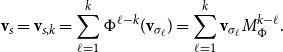 \begin{equation*}{\textbf{v}}_s= {\textbf{v}}_{s,k}= \sum_{\ell=1}^k \Phi^{\ell-k}({\textbf{v}}_{\sigma_\ell})= \sum_{\ell=1}^k {\textbf{v}}_{\sigma_\ell} M_\Phi^{k-\ell}.\end{equation*}
Note that from this
 ${\textbf{v}}_s$
, the contextualized vector representations for any other token
${\textbf{v}}_s$
, the contextualized vector representations for any other token
 $\sigma_m$
can then be easily retrieved by applying
$\sigma_m$
can then be easily retrieved by applying
 $\Phi^{k-m}$
to
$\Phi^{k-m}$
to
 ${\textbf{v}}_s$
. Now, given some permutation
${\textbf{v}}_s$
. Now, given some permutation
 $\Phi$
, we define the function
$\Phi$
, we define the function
 $\psi_{\scriptscriptstyle\Phi}$
which assigns to every
$\psi_{\scriptscriptstyle\Phi}$
which assigns to every
 ${\textbf{v}}_\sigma$
the matrix
${\textbf{v}}_\sigma$
the matrix
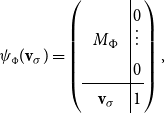 \begin{equation*}\psi_{\scriptscriptstyle\Phi}({\textbf{v}}_\sigma) = \left(\begin{array}{ccc|c}& & \ & 0 \\[-2mm]\ & M_\Phi & & \vdots \\& & & 0 \\\hline& {\textbf{v}}_\sigma & & 1 \\\end{array}\right),\end{equation*}
where
 $M_\Phi$
denotes the permutation matrix associated with
$M_\Phi$
denotes the permutation matrix associated with
 $\Phi$
as described in Section 3. Furthermore, we let
$\Phi$
as described in Section 3. Furthermore, we let
 \begin{equation*}\chi_{\scriptscriptstyle\Phi}(M) = (M(m,1) \quad M(m,2) \quad \cdots \quad M(m,m-1))\end{equation*}
(i.e., given a matrix M, extract the lowest row omitting the last entry). Then we obtain for a sequence
 $s=\sigma_1\ldots\sigma_k$
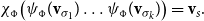 \begin{equation*}\chi_{\scriptscriptstyle\Phi}\big( \psi_{\scriptscriptstyle\Phi}({\textbf{v}}_{\sigma_1}) \ldots \psi_{\scriptscriptstyle\Phi}({\textbf{v}}_{\sigma_k})\big)={\textbf{v}}_s.\end{equation*}
Proof. The statement is a direct consequence of the following equality, which we show by induction on k:
 \begin{equation*}\psi_{\scriptscriptstyle\Phi}({\textbf{v}}_{\sigma_1}) \ldots \psi_{\scriptscriptstyle\Phi}({\textbf{v}}_{\sigma_k}) =\left(\begin{array}{c|c} & 0 \\[-2mm] M_\Phi^{k} & \vdots \\ & 0 \\\hline\sum_{\ell=1}^k {\textbf{v}}_{\sigma_\ell} M_\Phi^{k-\ell}& 1 \\\end{array}\right).\end{equation*}
For the base case, that is,
 $s = \sigma_1$
, the statement follows from the definition. For the induction step, we find
$s = \sigma_1$
, the statement follows from the definition. For the induction step, we find
 \begin{equation*}\psi_{\scriptscriptstyle\Phi}({\textbf{v}}_{\sigma_1}) \ldots \psi_{\scriptscriptstyle\Phi}({\textbf{v}}_{\sigma_k})=\big(\psi_{\scriptscriptstyle\Phi}({\textbf{v}}_{\sigma_1}) \ldots \psi_{\scriptscriptstyle\Phi}({\textbf{v}}_{\sigma_{k-1}})\big)\psi_{\scriptscriptstyle\Phi}({\textbf{v}}_{\sigma_k})\end{equation*}
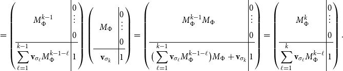 \begin{equation*}=\left(\begin{array}{c|c}& 0 \\[-2mm]M_\Phi^{k-1} & \vdots \\& 0 \\\hline\displaystyle\sum_{\ell=1}^{k-1} {\textbf{v}}_{\sigma_\ell} M_\Phi^{k-1-\ell}& 1 \\\end{array}\right)\left(\begin{array}{ccc|c}& & \ & 0 \\[-2mm]\ & M_\Phi & & \vdots \\& & & 0 \\\hline& {\textbf{v}}_{\sigma_k} & & 1 \\\end{array}\right)=\left(\begin{array}{c|c}& 0 \\[-2mm]M_\Phi^{k-1}M_\Phi & \vdots \\& 0 \\\hline\big(\displaystyle\sum_{\ell=1}^{k-1} {\textbf{v}}_{\sigma_\ell} M_\Phi^{k-1-\ell}\big)M_\Phi + {\textbf{v}}_{\sigma_k}& 1 \\\end{array}\right)=\left(\begin{array}{c|c}& 0 \\[-2mm]M_\Phi^{k} & \vdots \\& 0 \\\hline\displaystyle\sum_{\ell=1}^k {\textbf{v}}_{\sigma_\ell} M_\Phi^{k-\ell}& 1 \\\end{array}\right).\end{equation*}
 $\left.\right.$
 $\left.\right.$
q.e.d.
$\left.\right.$
q.e.d.
B. Proofs for Section 6
Proof of Theorem 1. If
 $\alpha$
is the zero vector, all scores will be zero, so we can let all
$\alpha$
is the zero vector, all scores will be zero, so we can let all
 $\hat{W}_h$
be the
$\hat{W}_h$
be the
 $(m+1)\times(m+1)$
zero matrix.
$(m+1)\times(m+1)$
zero matrix.
Otherwise let W be an arbitrary
 $m\times m$
matrix of full rank, whose first row is
$m\times m$
matrix of full rank, whose first row is
 $\alpha$
, that is,
$\alpha$
, that is,
 $e_1 W = \alpha$
. Now, let
$e_1 W = \alpha$
. Now, let
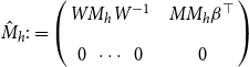 \begin{equation*}\hat{M}_h := \left(\begin{array}{c@{\quad}c}W M_h W^{-1} & M M_h \beta^\top \\[1ex]0\ \ \cdots\ \ 0 & 0\end{array}\right)\end{equation*}
for every
 $h\in \{1,\ldots,\ell\}$
. Then, we obtain
$h\in \{1,\ldots,\ell\}$
. Then, we obtain
 \begin{equation*}\hat{M}_{g} \hat{M}_{h} =\left(\begin{array}{c@{\quad}c}W M_{g} M_{h} W^{-1} & W M_{g} M_{h} \beta^\top \\[1ex]0\ \ \cdots\ \ 0 & 0\end{array}\right)\end{equation*}
for every
 $g,h\in \{1,\ldots,\ell\}$
. This leads to
$g,h\in \{1,\ldots,\ell\}$
. This leads to
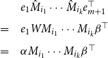 \begin{equation*}\begin{array}{l@{\quad}l}& e_1 \hat{M}_{i_1}\cdots\hat{M}_{i_k} e_{m+1}^\top \\[2pt]= & e_1 W {M}_{i_1}\cdots{M}_{i_k} \beta^\top \\[2pt]= & \alpha {M}_{i_1}\cdots{M}_{i_k} \beta^\top \\\end{array}\end{equation*}
 $\left.\right.$
q.e.d.
$\left.\right.$
q.e.d.
Proof of Proposition 2. Suppose
 $\Sigma=\{a_1,\ldots a_n\}$
. Given a word w, let
$\Sigma=\{a_1,\ldots a_n\}$
. Given a word w, let
 $x_i$
denote the number of occurrences of
$x_i$
denote the number of occurrences of
 $a_i$
in w. A linear equation on the letter counts has the form
$a_i$
in w. A linear equation on the letter counts has the form
 \begin{equation*}k_1x_1 + \ldots + k_nx_n = k\quad\quad\quad\big(k,k_1,\ldots,k_n\in\mathbb{R}\big)\end{equation*}
Now define
 $\mbox{$[\,\!\![$}{a_i}\mbox{$]\,\!\!]$} = \psi_+(\textbf{e}_i)$
, where
$\mbox{$[\,\!\![$}{a_i}\mbox{$]\,\!\!]$} = \psi_+(\textbf{e}_i)$
, where
 $\textbf{e}_i$
is the ith unit vector, that is, it contains a 1 at the ith position and 0 in all other positions. Then, it is easy to see that w will be mapped to
$\textbf{e}_i$
is the ith unit vector, that is, it contains a 1 at the ith position and 0 in all other positions. Then, it is easy to see that w will be mapped to
 $M=\psi_+(x_1 \quad \cdots \quad x_n)$
. Due to the fact that
$M=\psi_+(x_1 \quad \cdots \quad x_n)$
. Due to the fact that
 $\textbf{e}_{n+1} M = (x_1 \quad \cdots \quad x_n \quad 1)$
we can enforce the above linear equation by defining the acceptance conditions
$\textbf{e}_{n+1} M = (x_1 \quad \cdots \quad x_n \quad 1)$
we can enforce the above linear equation by defining the acceptance conditions
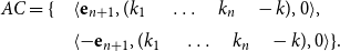 \begin{equation*}\begin{array}{r@{\quad}l}AC=\{ & \langle \textbf{e}_{n+1},(k_1\quad\ \ldots \quad k_n \quad -k),0 \rangle, \\& \langle {-}\textbf{e}_{n+1},(k_1\quad\ \ldots \quad k_n \quad -k),0\rangle\}.\end{array}\end{equation*}
 $\left.\right.$
q.e.d.
$\left.\right.$
q.e.d.
Proof of Proposition 3. This is a direct consequence of the considerations in Section 5.3 together with the observation, that the new set of acceptance conditions is trivially obtained from the old ones with adapted dimensionalities. q.e.d.
Proof of Proposition 3. The undecidable post correspondence problem (Post Reference Post1946) is described as follows: given two lists of words
 $u_1,\ldots,u_n$
and
$u_1,\ldots,u_n$
and
 $v_1,\ldots,v_n$
over some alphabet
$v_1,\ldots,v_n$
over some alphabet
 $\Sigma'$
, is there a sequence of numbers
$\Sigma'$
, is there a sequence of numbers
 $h_1,\ldots,h_m$
(
$h_1,\ldots,h_m$
(
 $1\le h_j\le n$
) such that
$1\le h_j\le n$
) such that
 $u_{h_1}\ldots u_{h_m} = v_{h_1}\ldots v_{h_m}$
?
$u_{h_1}\ldots u_{h_m} = v_{h_1}\ldots v_{h_m}$
?
We now reduce this problem to the emptiness problem of a matrix grammar. W.l.o.g., let
 $\Sigma' = \{a_1,\ldots,a_k\}$
. We define a bijection # from
$\Sigma' = \{a_1,\ldots,a_k\}$
. We define a bijection # from
 $\Sigma'^*$
to
$\Sigma'^*$
to
 $\mathbb{N}$
by
$\mathbb{N}$
by
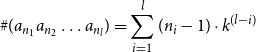 \begin{equation*}\#(a_{n_1}a_{n_2}\ldots a_{n_l})=\sum_{i=1}^l (n_i-1) \cdot k^{(l-i)}\end{equation*}
Note that this is indeed a bijection and that for
 $w_1,w_2\in \Sigma'^*$
, we have
$w_1,w_2\in \Sigma'^*$
, we have
 \begin{equation*}\#(w_1w_2) = \#(w_1)\cdot k^{|w_2|} + \#(w_2).\end{equation*}
Now, we define
 $\mathcal{M}$
as follows:
$\mathcal{M}$
as follows:
 \begin{equation*}\Sigma = \{b_1,\ldots b_n\}\quad\quad\mbox{$[\,\!\![$}{b_i}\mbox{$]\,\!\!]$} = \left(\begin{array}{c@{\quad}c@{\quad}c}k^{|u_i|} & 0 & 0 \\0 & k^{|v_i|} & 0 \\\#(u_i) & \#(v_i) & 1 \\\end{array}\right)\end{equation*}
 \begin{equation*}\begin{array}{r@{\quad}l}AC=\{ & \langle(0\quad 0 \quad 1),(1\quad -1\quad 0),0 \rangle, \\& \langle(0\quad 0 \quad 1),(-1\quad 1\quad 0),0 \rangle\}\end{array}\end{equation*}
Using the above fact about
 $\#$
and a simple induction on m, we find that
$\#$
and a simple induction on m, we find that
 \begin{equation*}\begin{array}{c}\mbox{$[\,\!\![$}{a_{h_1}}\mbox{$]\,\!\!]$}\ldots \mbox{$[\,\!\![$}{a_{h_m}}\mbox{$]\,\!\!]$} = \left(\begin{array}{@{}c@{\ \ }c@{\ \ }c@{}}k^{|u_{h_1}\!\ldots\! u_{h_m}|} & 0 & 0 \\0 & k^{|v_{h_1}\!\ldots\! v_{h_m}|} & 0 \\\#(u_{h_1}\!\ldots\! u_{h_m}) & \#(v_{h_1}\!\ldots\! v_{h_m}) & 1 \\\end{array}\right).\end{array}\end{equation*}
Evaluating the two acceptance conditions, we find them satisfied exactly if
 $\#(u_{h_1}\ldots u_{h_m}) = \#(v_{h_1}\ldots v_{h_m})$
. Since
$\#(u_{h_1}\ldots u_{h_m}) = \#(v_{h_1}\ldots v_{h_m})$
. Since
 $\#$
is a bijection, this is the case if and only if
$\#$
is a bijection, this is the case if and only if
 $u_{h_1}\ldots u_{h_m}= v_{h_1}\ldots v_{h_m}$
. Therefore,
$u_{h_1}\ldots u_{h_m}= v_{h_1}\ldots v_{h_m}$
. Therefore,
 $\mathcal{M}$
accepts
$\mathcal{M}$
accepts
 $b_{h_1}\ldots b_{h_m}$
exactly if the sequence
$b_{h_1}\ldots b_{h_m}$
exactly if the sequence
 $h_1,\ldots,h_m$
is a solution to the given post correspondence problem. Consequently, the question whether such a solution exists is equivalent to the question whether the language
$h_1,\ldots,h_m$
is a solution to the given post correspondence problem. Consequently, the question whether such a solution exists is equivalent to the question whether the language
 $L(\mathcal{M})$
is non-empty. q.e.d.
$L(\mathcal{M})$
is non-empty. q.e.d.
C. Discussion on cognitive plausibility of CMSMs
Recent research in psycholinguistics has focused on assessing the cognitive plausibility of distributional semantic models and word embeddings in VSMs. Mandera, Keuleers, and Brysbaert (Reference Mandera, Keuleers and Brysbaert2017) evaluate the performance of prediction-based models, for example, skip-gram and CBOW (Mikolov et al. Reference Mikolov, Chen, Corrado and Dean2013a), and count-based models, for example, word-context matrix, on predicting behavioral data on psychologically relevant tasks, such as semantic priming. In their experiments, Mandera et al. (Reference Mandera, Keuleers and Brysbaert2017) show that prediction-based models reflect human behavior better than count-based models on semantic-related tasks. They argue that learning in cognitive systems is incremental and all information is not simultaneously available to the learning system. Thus, prediction-based models, such as word2vec, which are also trained incrementally, are suggested as being much better grounded psychologically. Günther, Rinaldi, and Marelli (Reference Günther, Rinaldi and Marelli2019) also show that recent models, such as word2vec, show psychologically plausible learning mechanisms to obtain semantic meaning of words through semantic-related tasks. In this article, we proposed a learning technique for CMSMs, which is generally based on the distributional hypothesis. Incremental learning of the trained model is feasible by employing new data and information. Thus, these models are considered as prediction-based models, and their psychological plausibility can be analyzed systematically via psychologically relevant tasks, such as semantic priming and similarity/relatedness rating tasks. We leave this line of work as a future research in psycholinguistics.
Moreover, a recent study on vector-space DSMs by Sassenhagen and Fiebach (Reference Sassenhagen and Fiebach2019) shows that, when dealing with semantics, there is a correlation between the brain’s activity and semantic information in distributional models. They argue that a state in the human brain can be encoded in vectors, and therefore, vector mappings can be decoded from brain activity. More specifically, they show that there is a correspondence between the structure of brain activity and semantic vector spaces when processing language. With this in mind, suppose a state of a human’s brain at one specific moment in time can be encoded by a vector
 ${\textbf{v}}$
of numerical values. Then, an external stimulus or signal, such as a perceived word, will result in a transition of the mental state. Thus, the external stimulus can be seen as a function being applied to
${\textbf{v}}$
of numerical values. Then, an external stimulus or signal, such as a perceived word, will result in a transition of the mental state. Thus, the external stimulus can be seen as a function being applied to
 ${\textbf{v}}$
yielding as result the vector
${\textbf{v}}$
yielding as result the vector
 ${\textbf{v}}'$
that corresponds to the human’s mental state after receiving the signal. Therefore, it seems sensible to associate with every signal (in our case: word
${\textbf{v}}'$
that corresponds to the human’s mental state after receiving the signal. Therefore, it seems sensible to associate with every signal (in our case: word
 $\sigma$
) a respective function (a linear mapping), represented by a matrix
$\sigma$
) a respective function (a linear mapping), represented by a matrix
 $M_{\sigma}=\mbox{$[\,\!\![$}{\sigma}\mbox{$]\,\!\!]$}$
that maps mental states to mental states (i.e., vectors
$M_{\sigma}=\mbox{$[\,\!\![$}{\sigma}\mbox{$]\,\!\!]$}$
that maps mental states to mental states (i.e., vectors
 ${\textbf{v}}$
to vectors
${\textbf{v}}$
to vectors
 ${\textbf{v}}' = {\textbf{v}} M_{\sigma}$
).Footnote
l
Consequently, the subsequent reception of inputs
${\textbf{v}}' = {\textbf{v}} M_{\sigma}$
).Footnote
l
Consequently, the subsequent reception of inputs
 $\sigma$
,
$\sigma$
,
 $\sigma'$
associated with matrices
$\sigma'$
associated with matrices
 $M_{\sigma}$
and
$M_{\sigma}$
and
 $M^{\prime}_{\sigma}$
will transform a mental vector
$M^{\prime}_{\sigma}$
will transform a mental vector
 ${\textbf{v}}$
into the vector
${\textbf{v}}$
into the vector
 $({\textbf{v}} M_{\sigma})M^{\prime}_{\sigma}$
which by associativity equals
$({\textbf{v}} M_{\sigma})M^{\prime}_{\sigma}$
which by associativity equals
 ${\textbf{v}} (M_{\sigma} M^{\prime}_{\sigma})$
. Therefore,
${\textbf{v}} (M_{\sigma} M^{\prime}_{\sigma})$
. Therefore,
 $M_{\sigma}M^{\prime}_{\sigma}$
represents the mental state transition triggered by the signal sequence
$M_{\sigma}M^{\prime}_{\sigma}$
represents the mental state transition triggered by the signal sequence
 $\sigma\sigma'$
, as illustrated by Figure C1. Naturally, this consideration carries over to sequences of arbitrary length. This way, abstracting from specific initial mental state vectors, our matrix space
$\sigma\sigma'$
, as illustrated by Figure C1. Naturally, this consideration carries over to sequences of arbitrary length. This way, abstracting from specific initial mental state vectors, our matrix space
 $\mathbb{S}$
, introduced in Section 4, can be seen as a function space of mental transformations represented by matrices, whereby matrix multiplication realizes subsequent execution of those transformations triggered by external stimulus sequence, such as input token sequence. This way, we speculate the coherency of CMSMs with mental state progression; However, this needs to be confirmed by practical analysis in a similar way to the work by Sassenhagen and Fiebach (Reference Sassenhagen and Fiebach2019) in vector-space DSMs. Using matrices to represent these transitions restricts them to linear mappings. Although this restriction brings about benefits in terms of computability and theoretical accessibility, the limitations introduced by linearity assumption need to be further investigated.
$\mathbb{S}$
, introduced in Section 4, can be seen as a function space of mental transformations represented by matrices, whereby matrix multiplication realizes subsequent execution of those transformations triggered by external stimulus sequence, such as input token sequence. This way, we speculate the coherency of CMSMs with mental state progression; However, this needs to be confirmed by practical analysis in a similar way to the work by Sassenhagen and Fiebach (Reference Sassenhagen and Fiebach2019) in vector-space DSMs. Using matrices to represent these transitions restricts them to linear mappings. Although this restriction brings about benefits in terms of computability and theoretical accessibility, the limitations introduced by linearity assumption need to be further investigated.
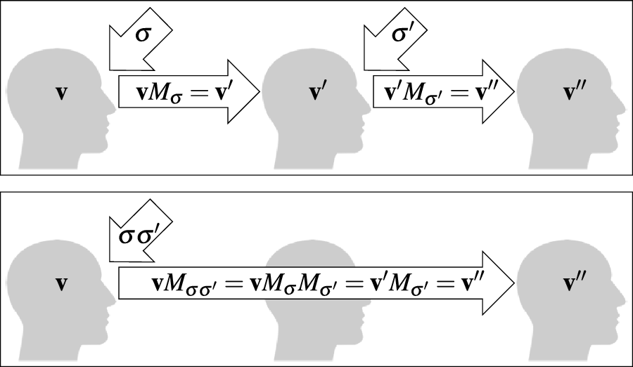
Figure C1. Matrices as cognitive state transformations.


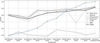


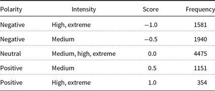


 Open access